the Creative Commons Attribution 4.0 License.
the Creative Commons Attribution 4.0 License.
 | 24 Jun 2020
Satellite-retrieved sea ice concentration uncertainty and its effect on modelling wave evolution in marginal ice zones
Takehiko Nose
Takuji Waseda
Tsubasa Kodaira
Jun Inoue
Ocean surface waves are known to decay when they interact with sea ice. Wave–ice models implemented in a spectral wave model, e.g. WAVEWATCH III® (WW3), derive the attenuation coefficient based on several different model ice types, i.e. how the model treats sea ice. In the marginal ice zone (MIZ) with sea ice concentration (SIC) < 1, the wave attenuation is moderated by SIC: we show that subgrid-scale processes relating to the SIC and sea ice type heterogeneity in the wave–ice models are missing and the accuracy of SIC plays an important role in the predictability. Satellite-retrieved SIC data (or a sea ice model that assimilates them) are often used to force wave–ice models, but these data are known to have uncertainty. To study the effect of SIC uncertainty ΔSIC on modelling MIZ waves during the 2018 R/V Mirai observational campaign in the refreezing Chukchi Sea, a WW3 hindcast experiment was conducted using six satellite-retrieved SIC products based on four algorithms applied to SSMIS and AMSR2 data. The results show that ΔSIC can cause considerable wave prediction discrepancies in ice cover. There is evidence that bivariate uncertainty data (model significant wave heights and SIC forcing) are correlated, although off-ice wave growth is more complicated due to the cumulative effect of ΔSIC along an MIZ fetch. The analysis revealed that the effect of ΔSIC can overwhelm the uncertainty arising from the choice of model ice types, i.e. wave–ice interaction parameterisations. Despite the missing subgrid-scale physics relating to the SIC and sea ice type heterogeneity in WW3 wave–ice models – which causes significant modelling uncertainty – this study found that the accuracy of satellite-retrieved SIC used as model forcing is the dominant error source of modelling MIZ waves in the refreezing ocean.
- Article
(10184 KB) - Full-text XML
- BibTeX
- EndNote


Satellite remote sensing and in situ observations reveal the Arctic Ocean sea ice has been declining in extent and volume (Maslanik et al., 2007; Kwok and Rothrock, 2009; Stroeve et al., 2012). Stroeve and Notz (2018) highlighted the emergence of consecutive monthly negative sea ice extent anomalies in recent years. From a practical viewpoint, this downward trend of sea ice decline opens trans-Arctic shipping routes connecting Europe and Asia for longer times of the year; potential global economic benefits of non-icebreakers accessing the Northern Sea Route and Northwest Passage are substantial (Stephenson et al., 2013; Bekkers et al., 2018). The increasing vessel traffic implies that adequate prediction capabilities will become crucial to assist ships in polar waters to circumnavigate hazards such as high winds and waves, collision with perennial sea ice, and sea-spray icing; however, Jung et al. (2016) state that the existing polar prediction systems need to be urgently enhanced to effectively manage the risks and opportunities associated with growing human activities. In this regard, the Polar Prediction Project (PPP) has contributed to advancing the predictive capabilities. While wave forecasting in polar oceans is still in its early years, the need for advancing wave forecast capacity will only grow in the emerging Arctic Ocean. This paper focuses on the effect of sea ice concentration (SIC) uncertainty on third-generation spectral wave model simulations in and near a marginal ice zone (MIZ). WMO (2014) defines the MIZ as “the region of an ice cover which is affected by waves and swell penetrating into the ice from the open ocean”. This study is primarily focused on the MIZ region at the interface between the open ocean and sea ice field.
Documented academic work on wave–ice interactions has a long history dating back as far as Greenhill (1886) (Squire, 2007; Mosig et al., 2015). When wind waves propagate through/under sea ice cover, the dispersion relation is modified and wave energy is attenuated due to non-conservative dissipation and a conservative scattering phenomenon. Stand-alone contemporary spectral wave models simulate wave–ice interactions using sea ice as forcing; in this space, the intensive field measurements of the Arctic Sea State and Boundary Layer Physics Program (Thomson et al., 2018) have made a solid contribution to the recent advance of The WAVEWATCH III® Development Group (WW3DG) (2019) wave–ice interaction parameterisations. Rogers et al. (2016), Cheng et al. (2017), Ardhuin et al. (2018), and Boutin et al. (2018) describe the development and optimisation of the latest WW3 parameterisations for wave evolution in sea ice cover. Despite the progress, Squire (2018) and Thomson et al. (2018) caution that accurately quantifying the wave decay and connecting the associated mechanisms over a large domain still remain a challenge because sea ice fields are notoriously heterogeneous; therefore, the wave–ice interaction parameterisation is a source of uncertainty when simulating wave evolution in MIZs. Recent developments of coupled wave–ice–ocean models on a pan-Arctic scale (Boutin et al., 2020; Roach et al., 2019; Zhang et al., 2020) reflect the growing interest in the ocean surface waves' role in the atmosphere, ocean, and sea ice dynamics: perhaps this indicates that advancing the wave–ice interaction physics is becoming a more pertinent issue to broader scientific communities.
Uncertainty in modelling ocean waves in ice-covered seas arises both from wave–ice interaction parameterisations and uncertainty in sea ice variables used as forcing: e.g. SIC and sea ice thickness (SIT). In particular, SIC retrieved from satellite radiometers (or sea ice models that assimilate satellite observations) forms the most fundamental input into wave–ice models and should have a profound effect on sea state predictions. Spatial distributions of SIC in the Arctic Ocean can be mapped daily based on satellite microwave radiometry, and they have been the primary source of sea ice trend and climatological studies; however, discrepancies among retrieval algorithms have been a long-known issue, and numerous intercomparison studies have investigated the effects of retrieval algorithms, and to a lesser extent instruments, on SIC estimates (Comiso et al., 1997; Meier, 2005; Andersen et al., 2007; Notz, 2014; Ivanova et al., 2015; Comiso et al., 2017; Chevallier et al., 2017; Roach et al., 2018; Lavergne et al., 2019). To date, there is no robust validation of any algorithm, so users are urged to understand strengths and weaknesses of the algorithms when using and interpreting the data (Ivanova et al., 2015; Comiso et al., 2017). The long-known SIC discrepancies imply there is uncertainty in the knowledge of true sea ice coverage (Notz, 2014). The uncertainty is potentially greater for MIZs in the refreezing ocean as satellite-derived SIC estimates are known to underestimate thin ice less than 35 cm (Heygster et al., 2014; Ivanova et al., 2015). Because the satellite-retrieved SIC has uncertainty, the choice of SIC product a modeller and model developers select is an error source. Since the latest WW3 wave–ice parameterisation developments used different sea ice forcing products, understanding the effect of SIC uncertainty on wave predictions is a relevant contribution and is the primary objective of this paper.
The expedition that inspired this study is introduced to close the preliminary section: the R/V Mirai Arctic Ocean observational campaign in the refreezing Chukchi Sea during November 2018 (JAMSTEC, 2018). A 12 d MIZ transect observation was conducted to capture daily changes in the sea ice field and the associated environmental conditions at the same geographical location. The observations showed firsthand how ocean surface waves propagate through a heterogeneous MIZ sea ice field. We began to inquire into how the sea ice field heterogeneity may affect a wave–ice model and how the satellite-retrieved SIC represents the observed sea ice field. The ensuing Sect. 2 introduces the methods employed to analyse the wave model uncertainties associated with SIC forcing including the R/V Mirai observation details. Section 3 discusses the SIC from a wave modelling perspective using the snapshot images of a sea ice field obtained during the MIZ transect observation. A wave hindcast experiment is conducted using various SIC products as forcing, for which the model results are compared with limited available in situ wave observations and two independent predictions as described in Sect. 4. The analysis is extended to the refreezing Chukchi Sea to examine the bivariate uncertainty data (model significant wave heights and SIC forcing) from a physical viewpoint of modelling wave decay and growth, which is discussed in Sect. 5. In this section, we also investigate the relative significance of the SIC uncertainty compared with the wave–ice interaction parameterisation uncertainty. Section 6 concludes and discusses the study findings.
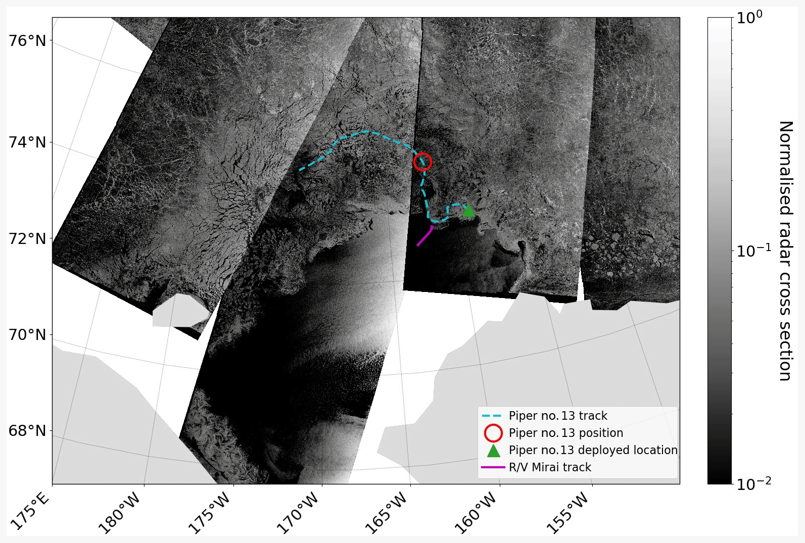
Figure 1Observation locations are overlaid on the mosaic of Sentinel-1 normalised radar cross section (NRCS) images (NOAA, 2019) acquired on 15 November 2018. The R/V Mirai track on this date is shown as the solid magenta line, and the Piper no. 13 drifting wave buoy track between 6 and 28 November is shown as the dashed cyan line. The green triangle shows the deployment location, and the red circle represents the buoy position on 15 November, 12:00.
2.1 R/V Mirai and drifting buoy observations
R/V Mirai MIZ transect observation
Regions in the Arctic Ocean, like the Chukchi Sea, that were inaccessible in November are now open for navigation, even for non-icebreakers, and R/V Mirai, a Japanese ice class vessel (JAMSTEC, 2019), carried out a late autumn voyage in 2018. R/V Mirai arrived in the Chukchi Sea on 4 November; after other ship time commitments, it began a 12 d transect observation that included an MIZ during daylight hours on 9 November. Daylight hours are limited at high latitudes during this time of the year, so sea ice observation was conducted generally between 19:00 and 00:00 UTC each day. The transect spanned roughly from 73.00∘ N, 198.00∘ E in the MIZ to 72.00∘ N, 194.00∘ E towards the central Chukchi Sea. Daily observation of the sea ice conditions at the same geographical locations for an extended period is rare if not unique because of exhaustive ship time required. The R/V Mirai transect on 15 November is overlaid on the mosaic of Sentinel-1A and B synthetic aperture radar (SAR) normalised radar cross section (NRCS) images (NOAA, 2019) captured on the same day in Fig. 1. Shipboard measurements used in this study include surface wind, sea surface temperature (SST), air temperature, and surface wind waves (WM-2 and Piper-C no. 15). The details of the R/V Mirai measurement systems are provided in Appendix A.
Drifting buoy wave measurement
Two drifting type wave buoys were also deployed during the R/V Mirai observational campaign. One failed within hours, but the other buoy, Piper no. 13, survived for 19 d after being deployed on 6 November 2018, 22:18; it was remotely switched to a sleep mode to preserve battery on 26 November, and the remote connection ceased on 5 December for some unknown reason. Hardware and on-board data processing were mostly the same as Nose et al. (2018) except Piper no. 13 produced bulk parameters at 15 min intervals, which were transmitted near real time via Iridium satellite communication. Piper no. 13 was deployed at 73.32∘ N, 201.09∘ E, and its track between 6 and 27 November is presented in Fig. 1 overlaid on the NRCS mosaic. The wave height is calculated as within the analysed range of a spectrum between the low and high cut-off frequencies, f_low and f_high, respectively. , where S is the variance density spectrum.
2.2 Satellite-retrieved sea ice concentration
SIC estimates from Earth-orbiting satellites are an indirect measurement calculated from microwave brightness temperatures. Although passive microwave radiation has low energy, brightness temperatures between sea ice and open ocean are distinguishable due to the difference in surface emissivity and physical temperatures. Microwave brightness temperatures measured from different frequency channels can account for the spatial and temporal variations of the ocean surface, so retrieval algorithms can be applied to produce SIC field estimates (Comiso et al., 2017).
Cavalieri et al. (1996–2018)Meier et al. (2018)Comiso (2017–2018)Hori et al. (2012)Spreen et al. (2008)Spreen et al. (2008)Table 1Details of satellite-retrieved SIC products used in this study.
Since the 1970s, a number of multichannel passive microwave radiometers have been in operation, and the sensors currently in operation (that are most used) for sea ice analysis are SSMIS and AMSR2. The key difference between the two sensors to derive the SIC spatial distribution is footprint resolution as the latter instrument has around 3–4 times higher resolutions for frequencies near 19, 37, and 89 GHz. For these two sensors, a large number of SIC retrieval algorithms have been developed primarily because different algorithms produce considerably different SIC estimates. This is evidenced by a long list of intercomparison studies (Comiso et al., 1997, 2017; Meier, 2005; Andersen et al., 2007; Notz, 2014; Ivanova et al., 2015; Chevallier et al., 2017; Roach et al., 2018; Lavergne et al., 2019).
A total of eight SIC products were selected for this uncertainty study based on four algorithms applied to SSMIS and AMSR2 data. Hereinafter, uncertainty of satellite-derived SIC ci for a set of data products is defined as follows:
where denotes the respective data products.
Four algorithms that appear most frequently in literature were selected: NASA Team (Cavalieri et al., 1984), bootstrap (Comiso, 1986), OSISAF, and ARTIST sea ice (Spreen et al., 2008). The selected products are summarised in Table 1, where the product abbreviations and data references are also provided.
A concise explanation for the selection of each product is given below.
-
NASA Team. The algorithm has been used for sea ice trend and climatological studies since the beginning of the satellite radiometry era. The SIC data used in this study are the original NASA Team algorithm applied to SSMIS data and the enhanced NASA Team 2 algorithm applied to AMSR2 data.
-
Bootstrap. Like NASA Team, the bootstrap algorithm has been used for sea ice trend and climatological studies for many years. The SIC data used in this study are the bootstrap algorithm applied to SSMIS and AMSR2 data.
-
OSISAF. This algorithm was selected because the highly reputable European Centre for Medium-Range Weather Forecasts (ECMWF) wave model (ECWAM) uses sea ice forcing based on the Operational Sea Surface Temperature and Sea Ice Analysis (OSTIA) system (Donlon et al., 2012) for which SIC is retrieved using the OSISAF algorithm applied to SSMIS data. We also analyse the AMSR2 data in this study.
-
ARTIST sea ice. This algorithm uses the 89 GHz frequency signal to produce high-resolution SIC estimates. This algorithm was selected as accurate higher-resolution forcing is generally desirable for numerical models. For this product, we only use the AMSR2 data but analyse two different grids: the pan-Arctic data with 6.250 km resolution and the regional Chukchi–Beaufort data with 3.125 km grid resolution.
The principle of all sea ice algorithms as described in Comiso (2007) is that measured radiative flux can be expressed as , where Ti and To are the brightness temperatures normally observed from 100 % ice cover and 100 % open water, respectively. Then, SIC can be expressed simply as , where the subscript b corresponds to observed ocean surface, and the ice-free surface is (Comiso, 2007). The accuracy of SIC is then dependent on the closeness of tuning brightness temperature tie points to the ice-free and fully-ice-covered ocean surface. The selection of frequency channels to derive polarisation ratios or differences (V and H) and gradient ratios (V polarisation) to retrieve SIC also dictates strengths and uncertainties of each algorithm. Technical details of the respective algorithms are described in the Table 1 data references.
2.3 WAVEWATCH III® spectral wave model
The effect of SIC uncertainty on MIZ wave predictions was investigated by a hindcast experiment using the Arctic Ocean wave model developed at the University of Tokyo (TodaiWW3-ArCS) based on WW3, which was introduced in Nose et al. (2018). Third-generation spectral wave models simulate the numerical evolution of waves as energy budgets based on the action density balance equation
The left-hand side concerns wave kinematics where N is the wave action density spectrum, which is a function of frequency σ, direction θ, x and y space, and time t, and c describes the propagation velocities in spatial and spectral coordinates. In deep water when neglecting currents, c is the group velocity cg. Source terms are on the right-hand side and the ones relevant to this study include the following: the wind input term swind, the wave dissipation term sdissipation, the non-linear interaction term snon-linear interactions, and the wave–ice interaction term sice. The sum of these source terms s is expressed based on the following default scaling in ice-covered waters:
Specifically to this study, ci relates to the satellite-retrieved SIC and sice to the ice type, i.e. how the model treats sea ice. The effects of sea ice on waves are represented via the modified dispersion relation , where . The real part kr is the physical wavenumber and alters the propagation speed of waves in a sea ice field (analogous to effects of shoaling and refraction by bathymetry), and the imaginary part ki is the exponential decay coefficient. ki is introduced in the model as sice=−2cgkiN for fully-ice-covered sea, i.e. ci=1, and the solution to is . There are five options for treating sea ice in WW3 denoted as IC1–5; ci provides the scaling in the linkage between sice and ICX as
where pn is the sea ice properties, e.g. effective shear modulus and effective viscosity. Therefore, the rate of attenuation depends on the wave period and sea ice properties and is moderated by ci, i.e. .
The wave–ice models implemented in WW3 that calculate kr to model ki are IC2, IC3, and IC5. IC2 calculates dissipation due to basal friction in the boundary layer below an ice sheet, which is modelled as a continuous thin elastic plate based on the work of Liu and Mollo-Christensen (1988). IC3 treats sea ice as a viscoelastic layer based on Wang and Shen (2010), which calculates the internal stress of the ice cover based on storage and dissipation. IC5 is a viscoelastic beam model based on Mosig et al. (2015). The dispersion relations of these models are provided in Appendix B. Ardhuin et al. (2018) and Boutin et al. (2018) (IC2) as well as Rogers et al. (2016) and Cheng et al. (2017) (IC3) describe the progress of these sice parameterisations using the refreezing Beaufort Sea data of Thomson et al. (2018). These wave–ice models can be combined with an energy-conservative scattering attenuation model denoted as IS1 and IS2 (Meylan and Masson, 2006; Dumont et al., 2011; Williams et al., 2013; Ardhuin et al., 2018; Boutin et al., 2018).
During the R/V Mirai cruise, sea ice in the MIZ was mainly grease, nilas, and pancake ice, so the hindcast experiment was conducted using the IC3 package (with the default parameters) as it has been designed for these ice types (Rogers et al., 2016; Cheng et al., 2017). Scattering is not expected to be the dominant process in this type of ice fields (Montiel et al., 2018), so it was not considered in the experiment. Regarding SIT forcing, a homogeneous input option with a value of 10 cm was applied; the constant forcing was applied so we can evaluate solely the Δci effect in the wave–ice models. A value of 10 cm was chosen because the MIZ transect observation was mostly characterised by new and young ice whose upper bound of SIT is of a similar order (Canadian Ice Service-Environment Canada, 2005).
swind and sdissipation parameterisations for TodaiWW3-ArCS were selected by comparing the two most commonly used physics packages ST4 (Ardhuin et al., 2010; Rascle and Ardhuin, 2013) and ST6 (Rogers et al., 2012; Zieger et al., 2015; Liu et al., 2019). We tested ST4 and ST6 against the 2016 September storm (Nose et al., 2018) – using ECMWF global reanalysis (ERA5) 10 m wind (U10) forcing – when TodaiWW3-ArCS and observations agreed well. The ST6 parameterisation showed marginally improved agreement using the default parameters; so all simulations used the ST6 swind and sdissipation parameterisations with ERA5 wind field forcing. The default snon-linear interactions, which is not affected numerically by sea ice, was used for all simulations.
TodaiWW3-ArCS, used in this study, has a horizontal resolution of 4 km, and its domain covers most of the Pacific side of the Arctic Ocean including the East Siberian, Chukchi, and Beaufort seas. The model boundaries connected to the seas of the Arctic Ocean were enclosed by ice cover during the November 2018 modelling period (corresponding to the R/V Mirai observation), so nesting was unnecessary. Similar to Rogers et al. (2016), we neglected swell penetration through the Bering Strait. The technical details of TodaiWW3-ArCS's geographical and spectral grids are provided in Appendix B.
ASI-3km and OSISAF-AMSR2 data were excluded for the wave hindcast experiment. The former has a regional coverage that is too small for the TodaiWW3-ArCS domain, and the OSISAF-AMSR2 data have noise in the open ocean, which yield erroneous wave simulation results when they are used as model forcing (as described in Appendix C). The remaining six satellite-retrieved SIC products in Table 1 were used as model forcing to examine wave modelling uncertainty, so the Δci wave hindcast experiment dataset has , where denotes the satellite-retrieved SIC forcing. Step-like changes in SIC from daily intervals are not ideal as forcing, so the SIC data were interpolated to match the model output frequency of hourly intervals. Unless specified otherwise, all other settings were default. The modelling period covers both R/V Mirai and Piper no. 13 observations and is from 5 to 25 November 2018 with a 5 d spin-up.
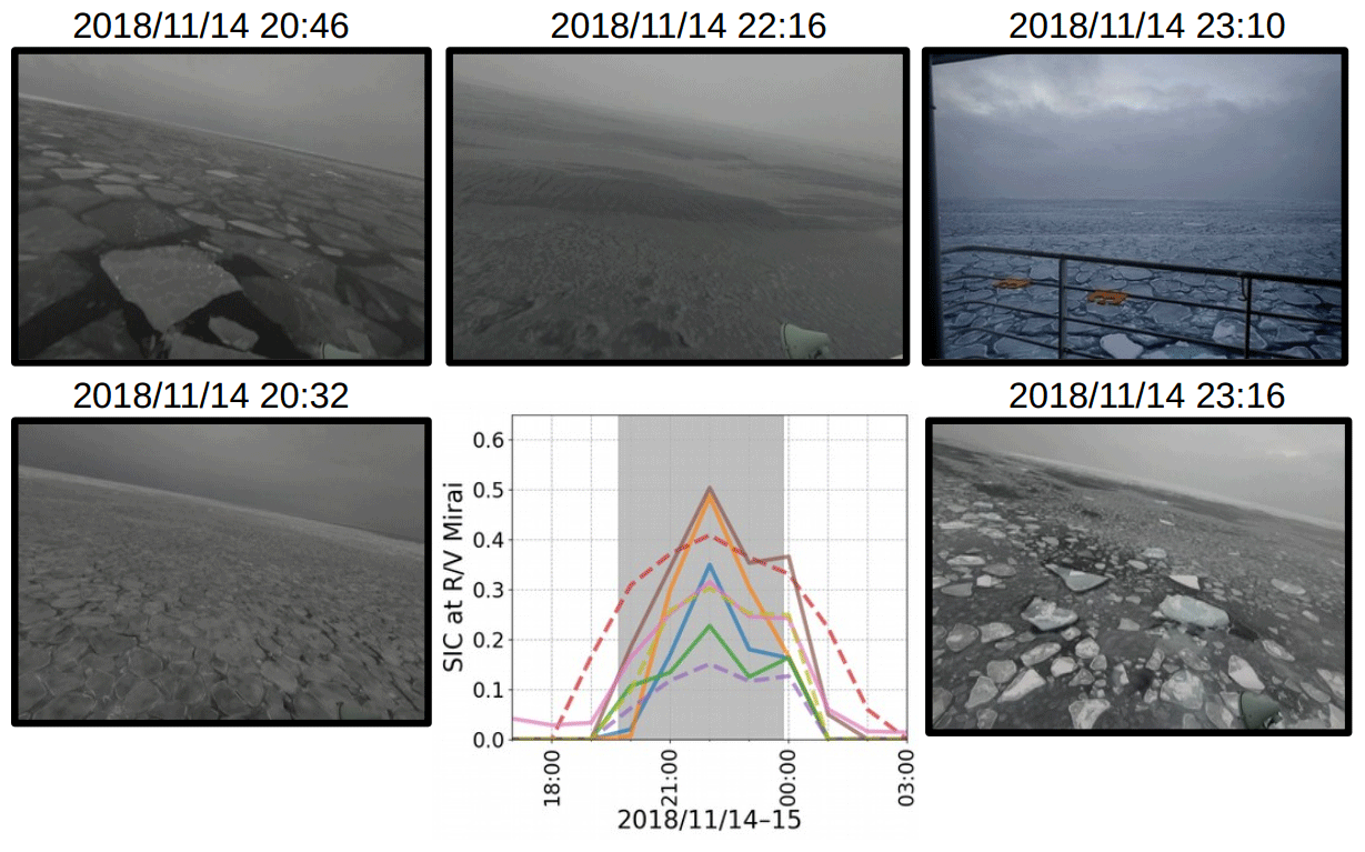
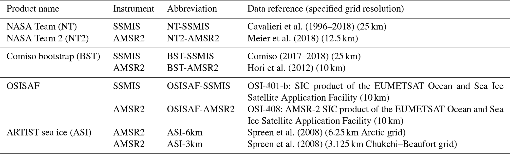
Figure 2Snapshot images taken from R/V Mirai of the sea ice field and the satellite-retrieved SIC estimates from eight products on 14 November 2018 during the on-ice wave event. The satellite-derived SIC was linearly interpolated in time to hourly intervals and bilinearly interpolated in space from respective native grids to the R/V Mirai positions using the Python SciPy interpolation package (Virtanen et al., 2020). The figure schematics of SIC estimates are as follows: ASI-3km (blue), ASI-6km (orange), BST-AMSR2 (green), BST-SSMIS (red), NT2-AMSR2 (purple), NT-SSMIS (brown), OSISAF-AMSR2 (pink), and OSISAF-SSMIS (olive), and SSMIS and AMSR2 are distinguished by dashed and solid lines, respectively. For the satellite-retrieved SIC figure legend, please refer to Figs. D2–D4. Grey highlighted times indicate when the vessel was in ice cover based on the ice navigator's logs: from the first (known) encounter of sea ice to the ship proceeding to the ice-free water.
It should be noted that when satellite-derived SIC data are used as forcing, the heat and momentum fluxes are distorted in the marine atmospheric boundary layer because the lower atmosphere and the ocean surface are no longer coupled. Inoue et al. (2011) evaluated surface heat transfer from three reanalysis products by focusing on how the models treat sea ice; they found the treatment of SIC is a key factor for the estimation of surface turbulent heat fluxes. Guest et al. (2018) have elucidated the ice edge jet generation mechanism based on the in situ data obtained in the refreezing Beaufort Sea. Undoubtedly, altering the sea ice field would feed back to the wind, but this is not captured in this wave hindcast experiment.
WMO (2014) defines SIC as “the ratio expressed in tenths describing the amount of the sea surface covered by ice as a fraction of the whole area being considered”. The so-called “area considered” presumably varies for different objectives. The length scale of O(10) km may be adequate for sea ice extent climatology, but for wave–ice interactions, the waves provide the scale in a phase-resolved sense. Satellite-retrieved SIC represents the fraction of ice-covered water over a large area, sufficiently large enough that the SIC represents a property of a continuum. In reality, the sea ice in the MIZ is granular, and ice floes jam due to horizontal convergence by Langmuir circulation, internal waves, and wind variability, resulting in a formation of features such as ice bands and wind streaks – with which waves likely interact distinctively.
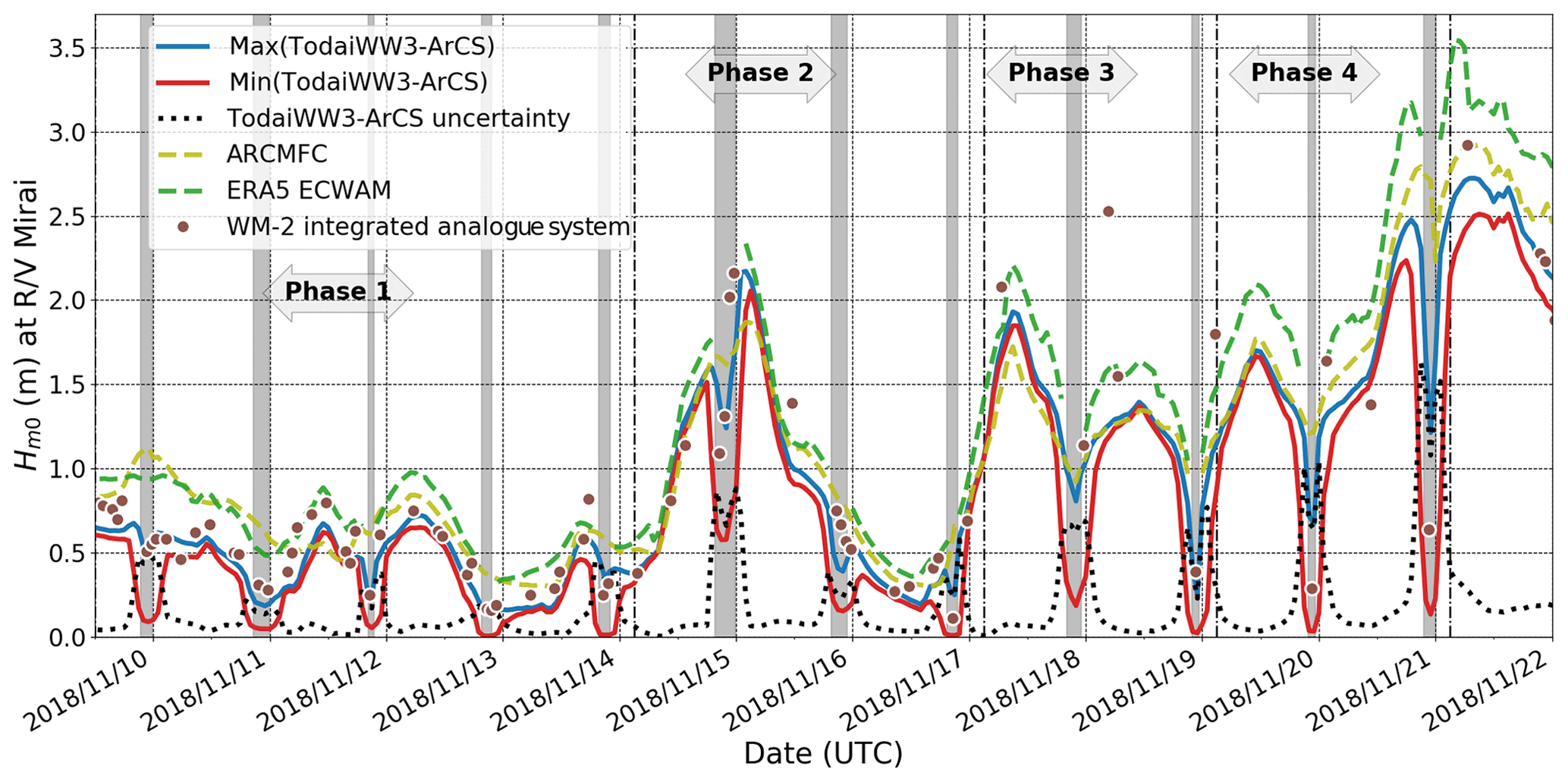
Figure 3 and values of TodaiWW3-ArCS estimates using various SIC products as sea ice forcing interpolated at R/V Mirai positions are shown during the MIZ transect observation. The figure also shows the WM-2 data when R/V Mirai ship speed was < 2 m s−1 (refer to Appendix A for more details). Two independent predictions from ERA5 ECWAM and the ARCMFC wave model are also presented. Grey highlighted times indicate when the vessel was in ice-covered sea based on the ice navigator's logs. Refer to Appendix D for details on phases.
On 14 November 2018, during the MIZ transect observation, R/V Mirai encountered moderate on-ice waves with an up to around 2.00 m propagating towards the ice edge (this estimate is consistent from both the shipboard wave data described in Appendix A and hindcast models as shown later). Figure 2 presents a series of snapshot images of the sea ice field during the encounter. R/V Mirai traversed over 10 km in the MIZ from the ice edge, and each image area extends at least over 1 km conservatively (using the crude distance to horizon calculation). These images depict the heterogeneous sea ice field, both in SIC and ice types, that waves propagate when they enter an MIZ. Because WW3 wave–ice interaction models are scaled according to (Eq. 4), subgrid-scale physics relating to the SIC and sea ice type heterogeneity is missing. As an example to account for SIC heterogeneity, we may write the subgrid-scale SIC as , where 〈ci,subgrid〉 is the grid scale. If we let the attenuation rate α be a function of SIC, the subgrid-scale attenuation may be expressed as however,
If the attenuation rate is non-linear, then so . The same logic may also apply to the sea ice types. It is plausible that the subgrid-scale distribution of SIC and sea ice types may be treated in a stochastic manner to provide meaningful mean values to the grid-scale model. For now, the missing formulation of subgrid-scale processes likely causes sizeable wave–ice model uncertainty. In existing parameterisations, SIC also affects the WW3 wave–ice model by means of scaling (Eq. 4). The Fig. 2 snapshot images are accompanied with SIC data from eight satellite-retrieved products described in Sect. 2.2 during this event. The SIC estimates interpolated at the R/V Mirai positions largely deviate among the products, characterising the uncertainty of the satellite-retrieved SIC. Moreover, the entire time series during the 12 d MIZ transect observation depicts Δci was persistent (Figs. D2–D4 of Appendix D). Hereafter, we show how large the effect of Δci on modelling MIZ waves can be, so much so that it overwhelms the choice of sice, e.g. ICX.

Figure 4Piper no. 13 wave data are presented with TodaiWW3-ArCS and using various SIC products as sea ice forcing interpolated at the Piper no. 13 positions. Two independent predictions from ERA5 ECWAM and the ARCMFC wave model are also presented.
Our goal is to understand Δci effects on wave–ice models, but adequate model accuracy, at least qualitatively, is needed for a meaningful uncertainty analysis. Because we lack a sufficient duration of robust in situ wave measurements, two independent numerical wave models that produce predictions in the Arctic Ocean, namely ERA5 ECWAM and the Arctic Monitoring and Forecasting Centre (ARCMFC) wave model, both based on WAM (wave model), were also included in the analysis. Comparisons with these high-quality models provide a guide on the TodaiWW3-ArCS performance. The ERA5 ECWAM data are made available on a 0.5∘ resolution grid on the Climate Data Store (Copernicus, 2019), and the model treats grid points with ci>0.30 as land using an ice mask. The ARCMFC wave model has a horizontal resolution of around 8 km and also used an ice mask. On 29 November 2018, shortly after our observation, their model was upgraded1 to simulate waves under sea ice cover based on the two-layer sea ice model of Sutherland et al. (2019): so we were unable to make use of their wave–ice interaction model data. The ARCMFC TOPAZ model provides the SIC and SIT forcing fields, which are kept constant from the initial state. Daily ARCMFC wave analysis data remapped to a 6.25 km polar stereographic grid were made available on ARCMFC (2019).
R/V Mirai MIZ transect observation
Figure 3 presents time series of interpolated at the R/V Mirai positions for all models during the MIZ transect observation (refer to Appendix D for the details on the environmental conditions during the MIZ transect observation). The figure also includes shipboard wave measurements from the WM-2 integrated analogue system (TSK Tsurumi Seiki Co., 2019) when the ship speed was < 2 m s−1 (refer to Appendix A for further explanation). Using Eq. (1), the model wave height uncertainty is denoted for six SIC forcing simulations. The figure shows that each time R/V Mirai sailed into ice cover, uncertainty in wave height generally increased. In the case of waves propagating towards the ice edge, waves decay at different timing depending on the sea ice edge location of the respective SIC data used, and the representation of the ice edge affects the fetch distance of off-ice wave growth as waves propagate towards open water. The model m occurred on 20 November 2018 during the off-ice wind condition, which is > 50 % of the open-water (of the TodaiWW3-ArCS and ARCMFC models). Because R/V Mirai slowed down in the MIZs, at least one WM-2 measurement was obtained in ice cover each day, and they generally lie within [), )]. Furthermore, when the open-ocean sea state is energetic, daily peak occurs as R/V Mirai sails into and out of the ice-covered water, indicating the model representation of the ice edges plays an important role.

Figure 5The 0.15 (solid) and 0.85 (dashed) SIC contours of OSISAF-SSMIS, BST-AMSR2, and ASI-3km for 15 November 2018, shown respectively as magenta, lime green, and cyan lines, are overlaid on the mosaic of Sentinel-1 NRCS images (NOAA, 2019) acquired on the same day. The solid black line above the figure legend provides a 200 km spatial reference.
Regarding the comparison of three different base models, ERA5 ECWAM consistently has a positive bias compared with other models except for the on-ice wave event on 14 November when they all agree reasonably well. For this event, both WM-2 and Piper-C no. 15 have comparable estimates of the measured peak as R/V Mirai was sailing out of the ice cover, which was around 2.00 m. The ERA5 ECWAM positive bias compared with other models is exacerbated when the strongest off-ice winds were recorded by R/V Mirai between 19 and 22 November. ARCMFC agrees slightly better with . These are evidenced in bias and root mean square deviation (RMSD) values calculated with respect to the ARCMFC : the ERA5 ECWAM has bias = 0.19 m and RMSD = 0.25 m, and the has bias = −0.11 m and RMSD = 0.21 m.
It is interesting to point out that using different sea ice forcing alone causes wave estimates to deviate in open water. This is also the case between the ERA5 ECWAM and ARCMFC models, which both use ECMWF wind forcing. The deviation of wave estimates in open ocean is more apparent during the off-ice wind conditions at the end of the transect observation period. A conjecture is that different treatments of sea ice in each model modified available fetch for which waves can be generated; for example, having open water to 0.30 SIC in ERA5 ECWAM, as it uses the ice mask, may simply increase the fetch distance at the R/V Mirai locations, which could result in a consistent positive bias compared with TodaiWW3-ArCS.
Piper no. 13 drifting buoy observation
Figure 4 is a Piper no. 13 equivalent of Fig. 3 with its observational data. Satellite-retrieved SIC for all products at the Piper no. 13 positions is provided in Fig. D5 of Appendix D. The buoy data are discussed first. It measured m for 2 d after being deployed on 6 November 2018. tapered off to around 0.20 m, but briefly rose to 0.60 m when the wind speed increased at around 12 November 2018, 00:00. Then, it drifted in ice cover with less wave penetration; no measurable wave signals propagated to Piper no. 13 as the measured spectra indicate noise except during the on-ice wave event between the late hours of 14 November and the early hours of 15 November. Peak wave periods, Tp, which is a frequency inverse corresponding to the maximum variance density, were consistently around 9 s; this is likely a true wave signal even though was only 0.05 m.
Regarding the wave hindcast, TodaiWW3-ArCS was the largest in open water and decreased with (i.e. mean of the TodaiWW3-ArCS simulations). In general, Piper no. 13 during 7 and 8 November is underestimated by all numerical models. When the wave energy tapered off between 8 and 11 November, both ERA5 ECWAM and ARCMFC model were overestimated. However, the episodic increase in wave energy on 11 and 12 November is reproduced in these models, albeit with a positive bias, whereas the TodaiWW3-ArCS simulations did not show any increase in the at the Piper no. 13 location. Close inspection of this event seems to indicate different treatments of sea ice in the models altered the fetch distance where the waves were generated: the models with ice masks (ERA5 ECWAM and ARCMFC) apparently have longer effective fetch and reproduced this episodic increase, whereas the wave generation was suppressed in the TodaiWW3-ArCS simulations. This indicates a possibility that TodaiWW3-ArCS underestimated the wave growth in low SIC waters: wave growth in ice-covered seas is discussed further in Sect. 5.1. There are no data shown for the ERA5 ECWAM and ARCMFC models after 12 November at Piper no. 13, presumably due to the ice masks. There are three occasions when all TodaiWW3-ArCS simulations slightly overestimate compared with the buoy data, which indicate the model attenuation rates may be too weak or SIC forcing is inaccurate.
This section demonstrated that simply changing SIC forcing alone produces considerable in the wave hindcast experiment at the observation sites. In the following section, we extend the wave hindcast analysis to the refreezing Chukchi Sea.
Figure 5 depicts 0.15 and 0.85 SIC contours on 15 November 2018 from three products: OSISAF-SSMIS, BST-AMSR2, and ASI-3km. They are overlaid on the NRCS mosaic of Sentinel-1 images acquired on the same day as NRCSs provide indication of true sea ice fields at a higher resolution. The difference among these contours in the MIZs is striking regardless of their footprint resolutions. The mosaic depicts sea ice edges that have a wavy, but highly non-linear, jagged form. For most of the ice edges, Fig. 5 shows OSISAF-SSMIS-derived 0.15 contours are smoother, whereas the BST-AMSR2 and ASI-3km contours appear to follow the sea ice edge concavity and convexity with a varying degree of closeness; ASI-3km appears to be qualitatively more consistent with the ice edges detected in the NRCS data. Figure 5 also shows the 0.85 SIC contours are somewhat qualitatively similar between OSISAF-SSMIS and ASI-3km; however, BST-AMSR2 and OSISAF-SSMIS 0.85 contours can be some 200 km apart, for example between 73.00∘ N, 190.00∘ E and 74.00∘ N, 185.00∘ E. Regions of low radar intensity that appear dark in the NRCSs are apparent in the disparate 0.85 SIC contours, which indicate SIC was not high in this area. As such, it does imply BST-AMSR2 overestimated the SIC for this date. Although not shown here, 0.50 SIC contours are inconsistent among all three products. It appears that ASI-3km generally captured qualitatively the SIC spatial variability shown in the NRCS data; however, this analysis suggests the satellite-retrieved SIC uncertainty can be considerable on a regional scale.

Figure 6ERA5 10 m wind speed (m s−1) and vectors to depict the forcing for southwesterly on-ice winds on 15 November 2018, 00:00 (a), and northeasterly off-ice winds on 21 November 2018, 21:00 (b).
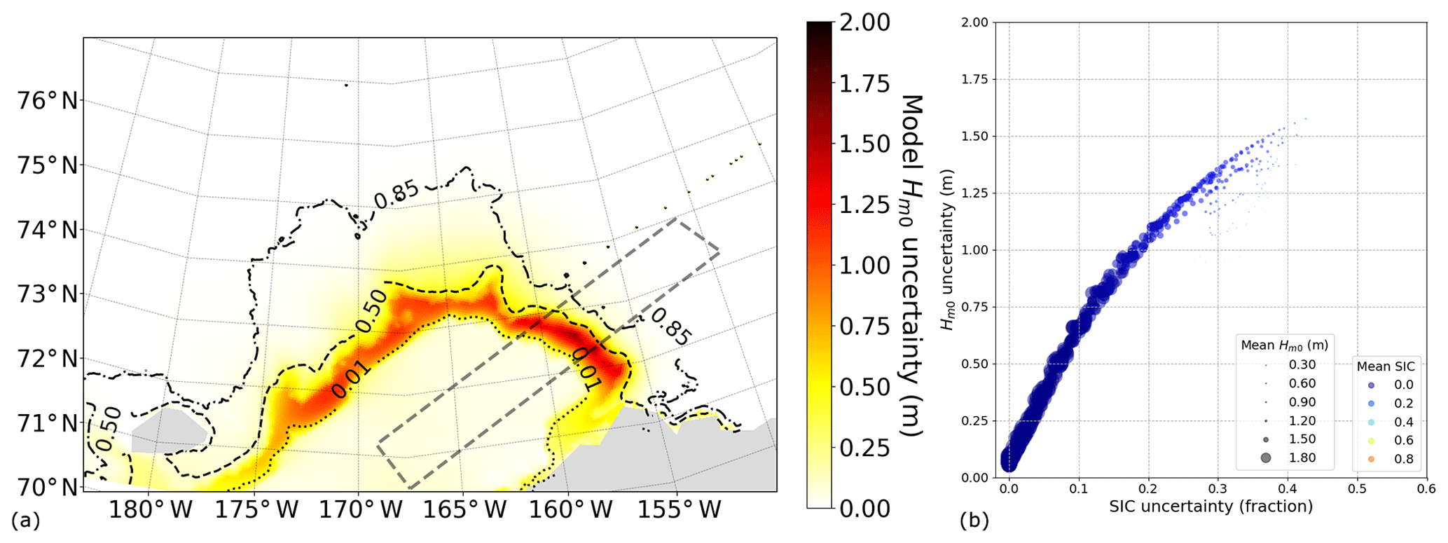
Figure 7TodaiWW3-ArCS simulation on 15 November 2018, 00:00, during southwesterly on-ice wind conditions as shown in Fig. 6a. (a) map with 0.01 (dotted), 0.50 (dashed), and 0.85 (dash-dotted) mean(ci) contours shown in black. (b) Bivariate model and Δci uncertainty data in an enhanced scatter plot for the quadrilateral area. The marker sizes are scaled by mean, and the marker colours indicate mean(ci).
5.1 On- and off-ice wave evolution in the refreezing Chukchi Sea MIZs
A more in-depth analysis is conducted here to understand how Δci affects the wave–ice interactions as implemented in WW3 from a physical viewpoint. At the most fundamental level, sea ice fields modify the fetch of the ocean: two cases are selected to analyse the effect of varying fetches on the attenuation and growth during on- and off-ice wave conditions on 15 November 2018, 00:00, and 21 November 2018, 18:00, respectively. The wind magnitudes and vectors for these cases are shown in Fig. 6. For the on-ice wave case, relatively strong small-scale southwesterly winds as depicted in Fig. 6a generated waves with an of about 2.00 m propagating towards the ice edge. When on-ice waves encounter ice cover, rapid attenuation is expected within O(10) km (Ardhuin et al., 2018; Squire, 2018), so the ice edge locations and the SIC variability near them affect the model simulation of wave decay. For the selected off-ice wave case, a low-pressure system over Alaska and a high-pressure system northwest of the Chukchi Sea generated sustained northeasterly winds over much of the Chukchi Sea as depicted in Fig. 6b, which generated open-water m. In this case, the ice edge and SIC field determine the fetch over which waves are generated, and as such, Δci introduces .
Owing to the heterogeneity of both the nature of wind that generates waves and the SIC field, there was no statistical association for the bivariate uncertainty data ( and Δci) even when the was normalised to wind forcing. In an attempt to elucidate the model uncertainties in the context of physical processes, a scatter plot is produced for both cases with the following visualisation technique: marker sizes are scaled to mean() as a bubble plot and each marker is colour coded according to mean(ci) (i.e. mean of the SIC forcing used in the TodaiWW3-ArCS simulations) like a colour-coded scatter plot. The former aims to emphasise the model data near the ice edge where the effects of wave attenuation and growth associated with Δci are most prominent. For simplicity, we refer to these figures herein as an enhanced scatter plot.
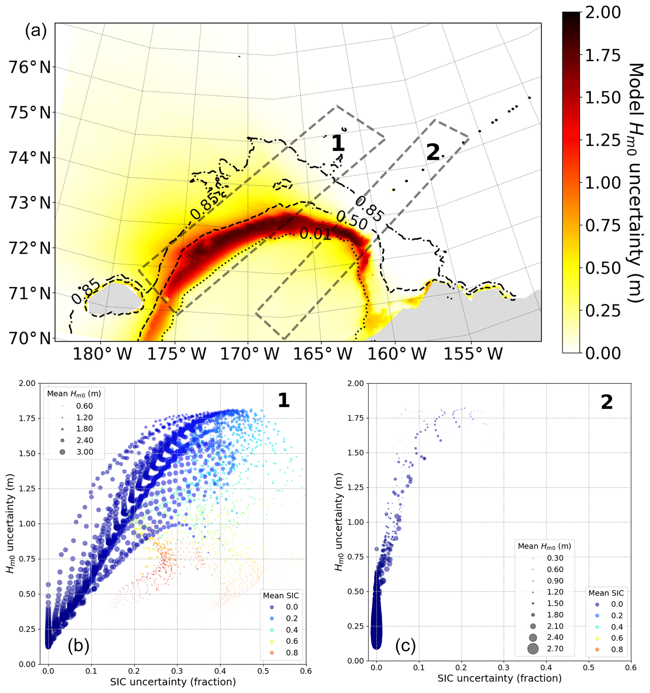
Figure 8TodaiWW3-ArCS simulation on 21 November 2018, 21:00, during northeasterly off-ice wind conditions as shown in Fig. 6b. (a) map with 0.01 (dotted), 0.50 (dashed), and 0.85 (dash-dotted) mean(ci) contours shown in black. (b) Bivariate model and Δci uncertainty data shown in an enhanced scatter plot for the quadrilateral 1 area where the wind forcing is oriented along the ice edge. (c) Bivariate model and Δci uncertainty data for the off-ice wave case for the quadrilateral 2 area. The schematics for panels (b) and (c) follow Fig. 7b.
Figure 7a depicts the spatial distribution of the model for the on-ice wave case with 0.01, 0.50, and 0.85 mean(ci) contours. Not all ice edges are aligned to the on-ice wind orientation because of the ice edge geometry. On-ice wave analysis was, therefore, conducted for a strip of the model grid points roughly 100 km in width along the southwesterly on-ice wind orientation as depicted in a grey dashed quadrilateral. An enhanced scatter plot shown in Fig. 7b depicts bivariate uncertainty data corresponding to the model grid points along the on-ice wind orientation. There is a strong indication of a correlation between the Δci and model for this on-ice wave case. The correlated uncertainties imply that as on-ice waves approach and decay due to wave–ice interactions, larger discrepancies in the representation of SIC as forcing causes greater model .
Figure 7b also shows the inverse proportion of marker sizes and uncertainties. Smaller size markers have low mean(), so larger values occur when only one or two of have while the remaining due to waves being fully attenuated. The figure shows only blue and light-blue markers, which indicate the waves generated by the strong localised winds decayed with limited wave penetration no farther than mean(ci)=0.40. Furthermore, in theory, the cluster of data must approach the origin of the figure coordinate in the upwind open waters in the central Chukchi Sea. In other words, on-ice waves that are being generated numerically in the open water must satisfy and Δci=0. The reason they do not converge to the figure coordinate origin is that the Δci along the Siberian coast (not shown here) affects the waves in the upwind waters as indicated by very faint yellow shades in Fig. 7a.
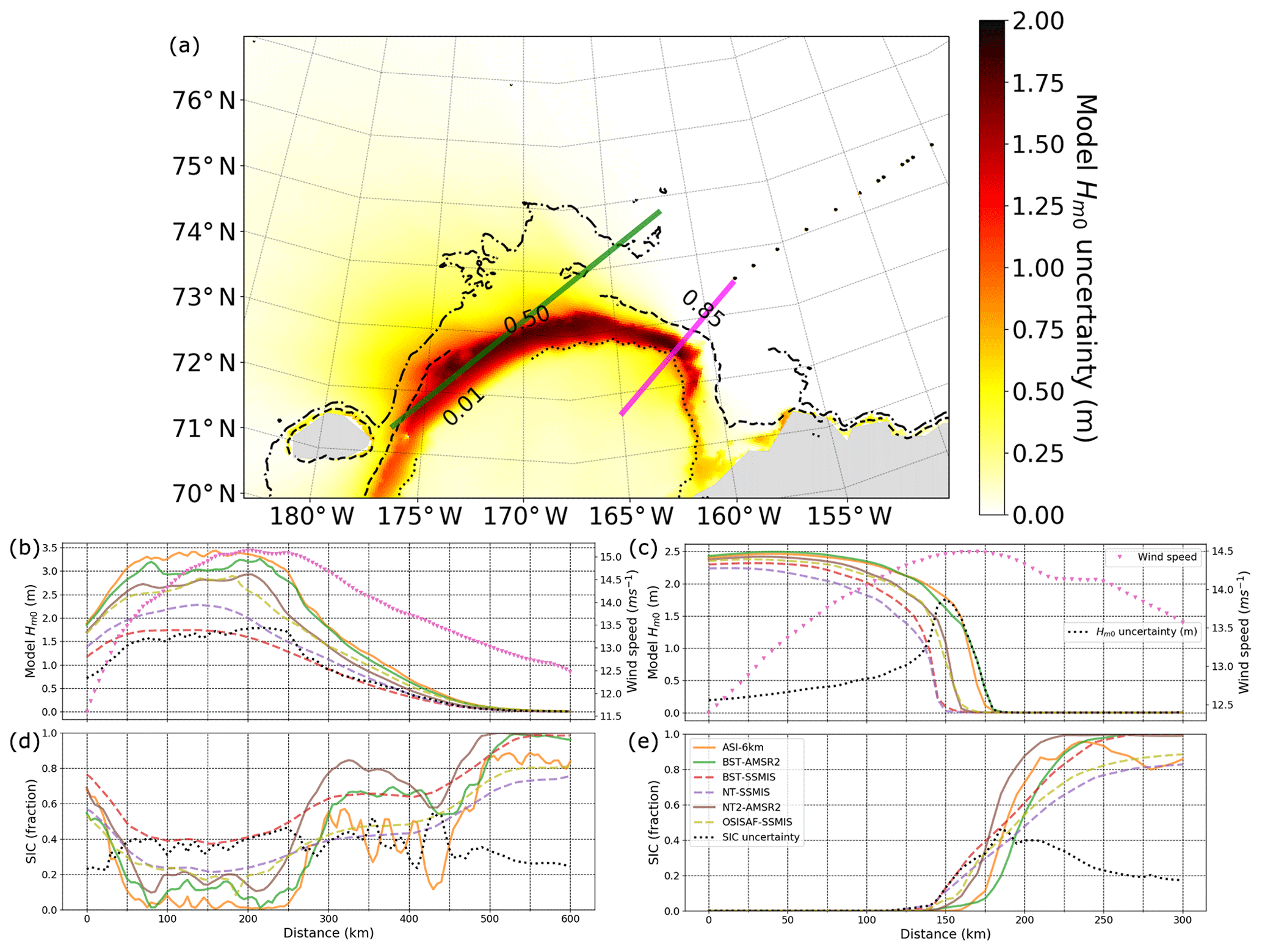
Figure 9TodaiWW3-ArCS simulation showing and SIC transects on 21 November 2018, 21:00, for the northeasterly off-ice wave case as shown in Fig. 6b. (a) uncertainty map with 0.01 (dotted), 0.50 (dashed), and 0.85 (dash-dotted) mean(ci) contours shown in black. (b, d) Model (b) and SIC ci (d) forcings along the green line are shown for the Δci hindcast experiment. (c, e) Model (c) and SIC ci (e) for an off-ice wave transect along the magenta line are shown for the Δci hindcast experiment. The figure schematics of SIC forcing follow Fig. 2. Magenta markers indicate the wind forcing magnitude, and dotted black lines represent and Δci.
Analysis of the off-ice case is carried out in a similar manner. The data bound by quadrilateral 2 as shown in Fig. 8a reflect the model grid points with the northeasterly off-ice wind conditions. Although the correlation is not as high as the on-ice wave case (with higher scatter for Δci>0.10), the enhanced scatter plot in Fig. 8c shows that the bivariate uncertainty data are correlated for the off-ice wave case as well. Analogous to the on-ice wave case, high can occur near the ice edge when only one or two simulations have the SIC forcing representing open-water conditions, while the wave growth is suppressed for the remaining simulations due to higher SIC. This effect is depicted in Fig. 9c and e, which shows TodaiWW3-ArCS and ci along a transect of the quadrilateral 2 long axis. Along this transect, ASI-6km and BST-AMSR2 have the most northeast ice edge, and the waves rapidly grow under the strong northeasterly wind forcing, whereas the higher SIC of the other simulations suppresses the wave growth. A distinct difference between the off- and on-ice wave cases regarding the Δci effect on wave–ice models is that remains in the downwind open ocean, whereas Δci→0. This is clearly shown in Fig. 8c, where when Δci=0, indicating the effect of Δci forcing on model can extend to the adjacent open water.
Off-ice wave evolution is a complex process because the fetch is not only controlled by the location of the ice edge, but also wave–ice interactions as implemented in WW3. The current numerical approach to simulate wind pumping energy into waves in ice cover is dictated by ci because waves grow when (Eq. 3). Li et al. (2017) found observational evidence of wind input to high-frequency wave energy in the Antarctic Ocean, and Kodaira et al. (2020) also obtained negative wave attenuation rates from drifting wave buoy observations between open water and grease ice in the refreezing Beaufort Sea; the negative values suggest possible wind input to waves in thin ice cover. As such, the off-ice is apparently also influenced by the cumulative effect of the Δci along the fetch distance affected by the wave–ice interaction parameterisations as implemented in WW3.
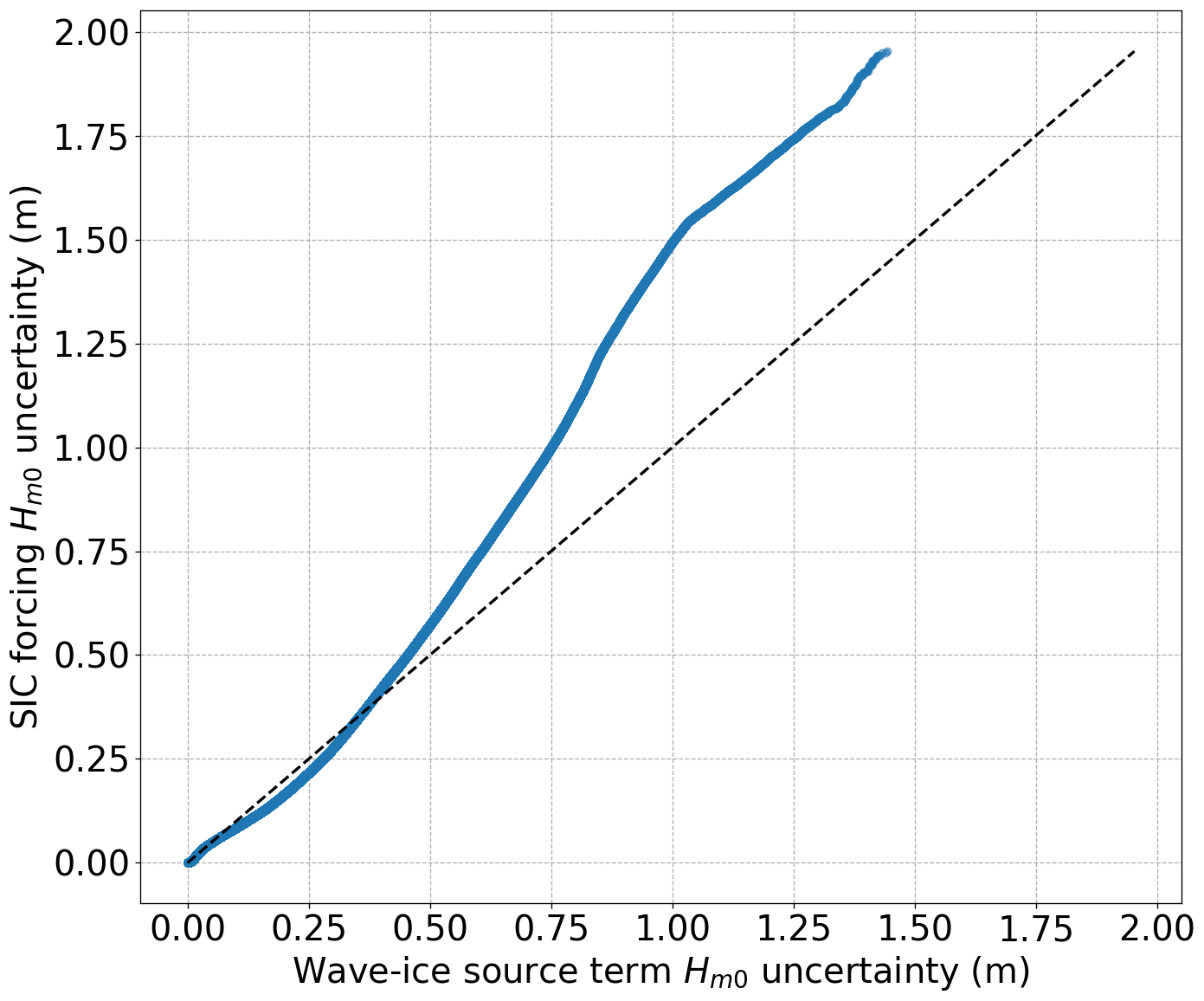
Figure 10A Q–Q plot depicting the distributions for Δci and sice uncertainty hindcast experiments.
Lastly, for both on- and off-ice wave cases, significant extends to the waters where the wind forcing is oriented along the ice edge; so the model data are briefly examined in the region of MIZs northeast of Wrangel Island, which is shown as quadrilateral 1 in Fig. 8a along the sea ice edge and northeasterly wind forcing orientation. This region has considerable Δci (not shown here) in a similar manner to Fig. 5, and the model is just as sizeable under the influence of high wind forcing. There is evidence of correlated bivariate uncertainty data in Fig. 8b, and a combination of on- and off-ice wave features for the respective enhanced plots discussed in the previous paragraphs is apparent. Deciphering the physical processes is complicated; however, the bivariate uncertainty data along a transect illustrates how Δci and are related; Fig. 9b and d shows TodaiWW3-ArCS ci and for a cross section oriented along the ice edge (the long axis of quadrilateral 2) on 21 November 2018 18:00. The figure depicts that is > 1.50 m in the area where Δci was around 0.40; it can also be inferred that the effect of Δci is greater when mean(ci) is lower.
5.2 Relative significance of Δci compared with wave–ice interaction parameterisation uncertainty
The Δci hindcast experiment conducted in this study intentionally adopted the default IC3 source term parameters. As mentioned in Sect. 1, considerable progress in the WW3 wave–ice interaction parameterisations has been made owing to the Thomson et al. (2018) measurements. However, Ardhuin et al. (2018) also explain that observed wave attenuation could also be reproduced with many model forcing and parameter combinations, which as stated in the article is not unexpected because different wave–ice interaction processes are taking place along the wave propagation path. As discussed in Sect. 2.3, WW3 offers three physics-based sice parameterisations: IC2, IC3, and IC5. They are based on different attenuation mechanisms and dispersion relations (see Appendix B), but their default ice rheological parameters (as given in the manual or the WW3 regression test cases) also vary as apparently the sea ice parameters are context-based according to the manual. The three main parameters used to tune the IC2, IC3, and IC5 attenuation rate are as follows: eddy viscosity (m2 s−1) ν, ice density (kg2 m−3) ρ, and effective elastic shear modulus (Pa) G, although G is not used in IC2. The default ρ values are consistent for these sice parameterisations. The default ν values are , 1.0, and 5.0×10⁷ for IC2, IC3, and IC5, respectively, and the default G values are 1.0×10³ and 4.9×10¹² for IC3 and IC5, respectively. Rogers et al. (2016) adopted G=0 assuming it is negligible in nilas and pancake ice fields. Based on the enormous range of tunable parameters and other factors described in this paragraph, the sice parameterisation is an apparent uncertainty source. To evaluate the relative significance of Δci, we compared the results with the wave–ice interaction source term uncertainty (sice uncertainty) for the modelling period between 5 and 25 November 2018. The sice uncertainty wave hindcast experiment was conducted using IC2, IC3, and IC5 based on the same model setup described in Sect. 2.3, except all three simulations used BST-AMSR2 as SIC forcing.
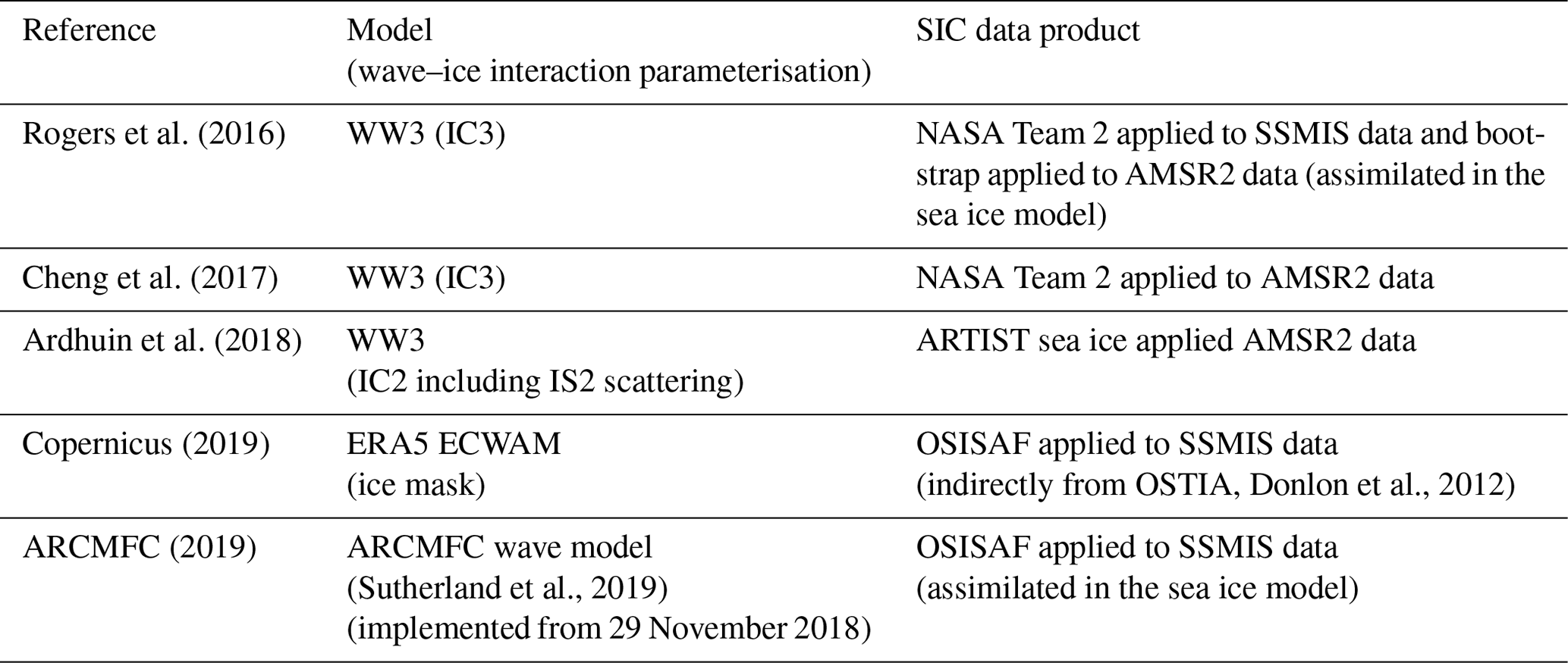
Rogers et al. (2016)Cheng et al. (2017)Ardhuin et al. (2018)Copernicus (2019)Donlon et al., 2012ARCMFC (2019)(Sutherland et al., 2019)Table 2A list of SIC data products used for various wave–ice interaction modelling studies.
A pair of datasets were derived for the Δci and sice uncertainty wave hindcast experiments. They were collated for the entire simulation period within the model domain shown in Fig. 7a. Uncertainty distributions are visualised in a Q–Q plot by simply sorting each dataset, and this is shown in Fig. 10. The figure depicts that ) values were 1.95 and 1.44 m for the Δci and sice uncertainty experiments, respectively. Although both uncertainties are considerable, Δci overwhelmed the sice uncertainty. The robustness of this result was examined via SIT forcing sensitivity analysis. From a physical viewpoint, the choice of 10 cm was made to match the observed sea ice types during the R/V Mirai MIZ transect observation: for the SIT sensitivity analysis, we adopted 50 cm. From a wave–ice modelling perspective, SIT effectively serves as a tuning parameter when forced as a homogeneous field. For example, the attenuation rate ki of IC2 as shown in Appendix B has SIT in the form of (1+krM) in the denominator: (Liu and Mollo-Christensen, 1988), where hi is the SIT, and ρ and ρw are the ice and sea water density. If we take a deep water wavelength corresponding to a 7 s wave period, changing the SIT from 10 to 50 cm increases the ki by at most 3 %. ki sensitivity to SIT examined in Wang and Shen (2010) and Mosig et al. (2015) (IC3 and IC5) appears more sensitive; as such, sensitivity analysis was warranted for our model. Repeating the Δci and sice uncertainty experiments with 50 cm SIT, ) values increased respectively to 2.34 and 1.95 m, but the Δci remained as the dominant error source. It is noted that IC3 was most affected by the SIT change for the equivalent transects of Fig. 9 (not shown here). Even though there was no event during the study period when scattering was expected to be the dominant process (the implication of this is given in Sect. 6), sensitivity of the finding to scattering was also examined (not shown here) by combining IS2 scattering with IC2 and IC3 with the default parameters. The result that Δci overwhelms the sice uncertainty remained robust for the study period. Lastly, sensitivity to the choice of SIC forcing used in the sice uncertainty experiment was examined by using ASI-6km instead of BST-AMSR2: Δci again remained as the dominant error source.
Table 2 is a list of SIC forcing used in the recent WW3 sice developments as well as the forcing of the wave models analysed in Sect. 4. Some studies employed numerical sea ice models or considered various sources and assessed their accuracy/suitability. It is interesting to learn that each wave–ice modelling study used different satellite-retrieved SIC data.
The WW3 wave–ice model used in this study simulates the wave attenuation in ice-covered seas based on , where ki represents the exponential decay coefficient (Eq. 4). It is worthy to note that the notion of exponential wave decay in ice cover is changing as field evidence and numerical studies enlighten the wave–ice community with new insights – e.g. Kohout et al. (2014) and Boutin et al. (2018). We investigated the effect of the satellite-retrieved SIC uncertainty Δci on modelling waves in the refreezing Chukchi Sea MIZ using six SIC datasets based on the four commonly used retrieval algorithms: NASA Team, bootstrap, OSISAF, and ARTIST sea ice. This Δci wave hindcast experiment revealed Δci causes model wave height uncertainty , and there is evidence that bivariate uncertainty data ( and Δci) are correlated, although off-ice wave growth is more complicated due to the cumulative effect of Δci along an MIZ fetch.
The relative significance of Δci was examined by comparing the distribution of the Δci experiment with that of the wave–ice interaction term sice uncertainty experiment, which comprised three TodaiWW3-ArCS simulations using the physics-based IC2, IC3, and IC5 sice parameterisations. Both uncertainties were considerable during the simulation period with maximum values of 1.95 and 1.44 m, respectively; however, the result showed that Δci overwhelms the sice uncertainty. This result is found to be robust based on the sensitivity analyses that tested the SIT forcing and the inclusion of scattering. Despite the WW3 wave–ice models missing the subgrid-scale physics relating to sea ice field heterogeneity (e.g. Eq. 5), this study found that the accuracy of satellite-retrieved SIC used as model forcing is the dominant error source of modelling MIZ waves in the refreezing ocean. The study outcome suggests wave–ice model tuning may not be as effective at this time when the knowledge of the true SIC field is too uncertain. It is noted that the conditions in which the scattering would likely be the dominant process were not observed during the study period. As such, the effect of Δci for such waves remains to be resolved.
Future improvements on the wave–ice models should come from two approaches: continual developments of parameterised physics on the regional and pan-Arctic scale and working on a subgrid-scale physical model on the other end. Solid and robust observational evidence through remote sensing and shipboard measurements is likely the key to connecting these two ends.
R/V Mirai is equipped with two anemometers that were located on the foremast at 25 m elevation, and indicative wind conditions at the ship positions were derived from 10 min vector moving averages of 6 s interval instantaneous true wind speed and direction. SST was measured 1 m below the sea surface with a further 5 m inlet to the gauge while air temperatures were measured on the foremast at 23 m elevation.
Shipboard waves were obtained based on two methods: a microwave radar system (WM-2) (TSK Tsurumi Seiki Co., 2019) at the bow and stern of the ship; and a nine-axis inertial moment unit (IMU) (Piper-C no. 15), which is a device similar to the one used by Kohout et al. (2015). WM-2 has a sampling frequency of 2 Hz and collects raw sea surface elevation for 1152 s at 35 min past each hour, and its integrated analogue system removes hull agitation and carries out Doppler correction. Bulk parameters like the significant wave height and period are produced based on the zero-crossing method. Wave observations during the campaign from the WM-2 integrated analogue system (TSK Tsurumi Seiki Co., 2019) were significantly affected by Doppler correction errors. Collins III et al. (2015) have shown shipboard measurements are less affected by this effect when ship speed is < 3 m s−1. Applying a 2 m s−1 ship speed threshold greatly reduced conspicuously spurious data, and these data were used as indicative wave heights in this study (e.g. Fig. 3). Piper-C no. 15 on board the vessel relies on an IMU. The processing method is consistent with Kohout et al. (2015) except 15 min intervals were used instead of 1 h. Waves in the Chukchi Sea during the study period were dominated by wind seas, which have shorter wavelength relative to the ship dimensions. These waves are impeded by R/V Mirai's hull, so the shipboard Piper-C no. 15 has limitations on measuring wind seas. The response amplitude operator of R/V Mirai and the WM-2 data can be combined in theory to transfer IMU's high-frequency signals to true surface elevations, but post-processing remains ongoing work. Although most of the Piper-C no. 15 data did not reflect the true wave field, the peak Piper-C no. 15 of 2.00 m during the on-ice wave event on 14 November 2018 agreed with the peak WM-2 ; this value is also comparable with the ERA5 as well. This provides confidence that the waves observed during this event were at least around 2.00 m.
The TodaiWW3-ArCS geographical grid at high latitudes was based on the curvilinear grid implemented by Rogers and Campbell (2009) with a polar stereographic projection of 75∘ N latitude (produced by MathWorks MATLAB's polarstereo_inv function). The model domain coverage on the polar stereographic grids is as follows: the easting extent is between −800 and 1512 km, and the northing extent is between 520 and 2904 km. The geographical grid was defined using the International Bathymetry Chart of the Arctic Ocean bathymetry (Jakobsson et al., 2012) and the Global Self-consistent, Hierarchical, High-resolution Geography shoreline data (Wessel and Smith, 1996), and there are approximately 301 535 sea point cells. The spectral grid was configured with 36 directional and 35 frequency bins, with the latter ranging from 0.041 to 1.052 Hz.
The WW3 wave–ice model dispersion relations for IC2, IC3, and IC5 are provided here. IC2 is based on the work of Liu and Mollo-Christensen (1988), and the dispersion relation is defined as follows according to the WW3 manual:
where
hi is the SIT, ρ and ρw are the ice and sea water density, ν is the viscosity, E is the Young modulus of elasticity, ϕ is the Poisson ratio, and P is the compressive stress in the ice pack.
IC3 is based on Wang and Shen (2010), and the dispersion relation is concisely shown in Eq. (4) of Cheng et al. (2017) as follows:
where
G is the shear modulus.
IC5 is based on Mosig et al. (2015), and the dispersion relation is defined as follows according to the WW3 manual:
where
The OSISAF-AMSR2 SIC estimates during the November 2018 study period consist of prevalent erroneous estimates in the open ocean. At the R/V Mirai positions, inaccurate SIC is estimated for 14 and 20 November 2018 when R/V Mirai was not in ice cover. These estimates are noise because R/V Mirai has strenuous restrictions when sailing in ice-covered seas and the sightings of sea ice are logged by the crew and the experienced ice navigator. This is also supported by the wave model as the TodaiWW3-ArCS simulation using OSISAF-AMSR2 as forcing calculates interpolated at R/V Mirai as 0 m for the 14 November on-ice event as shown in Fig. C1. There are also apparent errors on 20 November. The open-ocean OSISAF-AMSR2 SIC estimates for 14 and 20 November are shown in Fig. C2.
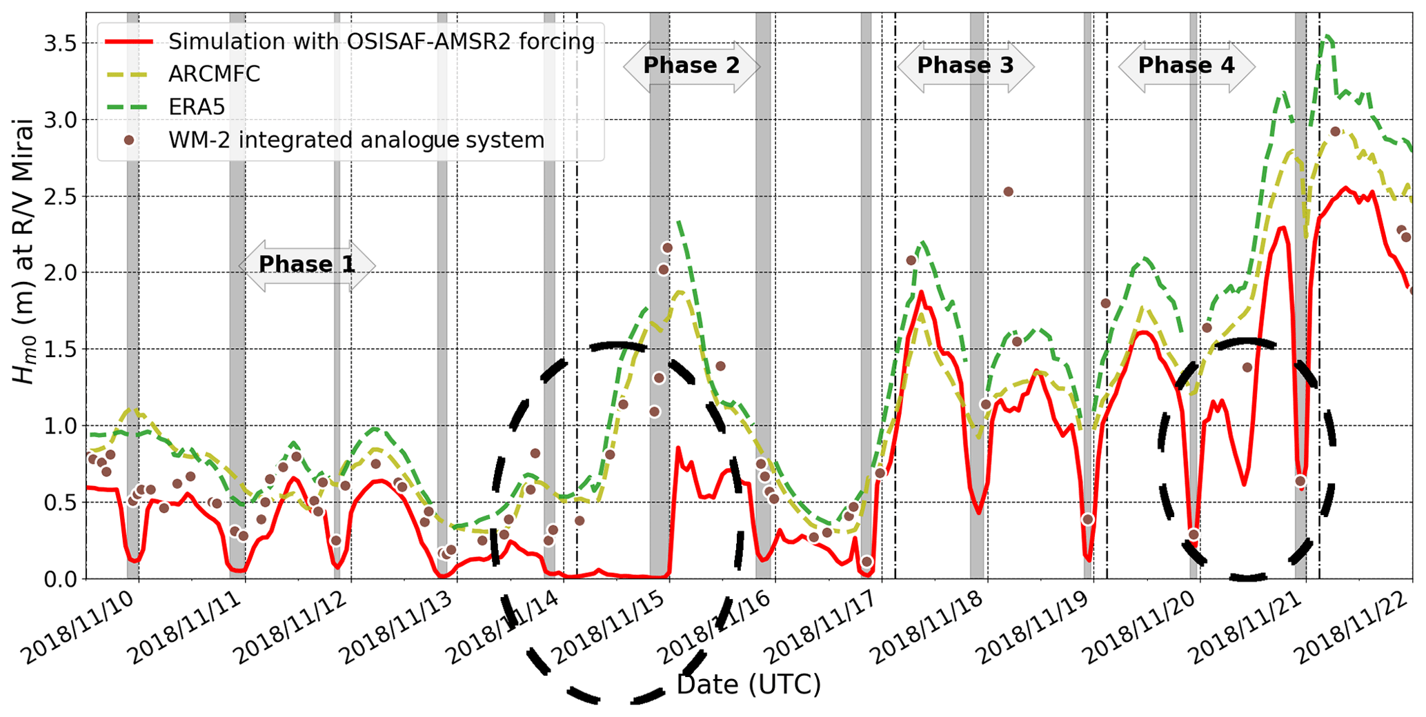
Figure C1The TodaiWW3-ArCS estimates using the OSISAF-AMSR2 SIC as forcing interpolated at R/V Mirai positions are shown during the MIZ transect observation. The figure also shows the WM-2 data when R/V Mirai ship speed was < 2 m s−1. Two independent predictions from ERA5 ECWAM and the ARCMFC wave model are also shown. The dashed black circles indicate times when the erroneous SIC forcing caused inaccurate estimates of at the R/V Mirai position. Grey highlighted times indicate when the vessel was in ice-covered seas based on the ice navigator's logs: from the first (known) encounter of sea ice to the ship proceeding to the ice-free water.
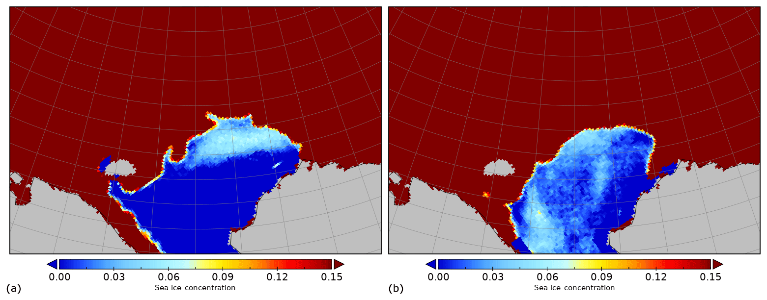
Figure C2Apparent OSISAF-AMSR2 SIC noise in the open water during the R/V Mirai MIZ transect observation. SIC estimates on 15 November (a) and 20 November 2018 (b).
This appendix describes the environmental conditions during the MIZ transect sea ice observation conducted by R/V Mirai in the refreezing Chukchi Sea, which is described in Sect. 2.1. It also provides the comparison of eight satellite-retrieved SICs at the observation locations including those at the Piper no. 13 drifting wave buoy.
R/V Mirai began the 12 d sea ice observation on 9 November 2018. Coinciding with this schedule, the transect waters began to refreeze and became consolidated ice cover at the start and (several days after) end of the observation period. The sea ice observation is grouped in four phases as distinct ocean surface features were captured from four meteorological conditions the ship encountered. Figure D1 presents the shipboard-measured wind and SST data as well as bilinearly interpolated (in space) ERA5 10 m wind speeds. During the first few days between 9 and 13 November 2018 (Phase 1), gradual sea ice growth was observed both in extent and ice cake/floe sizes under generally calm surface conditions. On 14 November, the most significant on-ice wind event during the transect period occurred. The peak wind speed measured by R/V Mirai was 18 m s−1, and > 10 m s−1 winds persisted for roughly 18 h at the ship location. WM-2 and Piper-C no. 15 both peaked at > 2.00 m in ice cover, indicating energetic sea state of this event. The MIZ was mostly broken up ice fields on the following day, which was followed by the most apparent sea ice advance on 16 November as a seemingly dense ice field was encountered. We have grouped this period, Phase 2, as the on-ice event and aftermath.
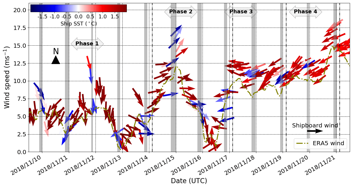
Figure D1Shipboard wind and SST and bilinearly interpolated ERA5 10 m winds at the R/V Mirai position. Grey highlighted times indicate when the vessel was in ice cover based on the ice navigator's logs.
During 17 and 18 November, sea ice observation was mostly open water; our conjecture is the sea ice disappeared by horizontal advection, but there is insufficient evidence to simply discard rapid melting or other processes. This period of minimal ice sighting is referred to as Phase 3. In the final Phase 4, SSTs along the transect waters began to warm despite the persistent and strengthening cold off-ice winds. Air temperatures along the MIZ transect on 18–20 November were < −10 ∘C, but the shipboard SSTs exceeded 0 ∘C for the entire MIZ transect waters the ship traversed on 20 November.
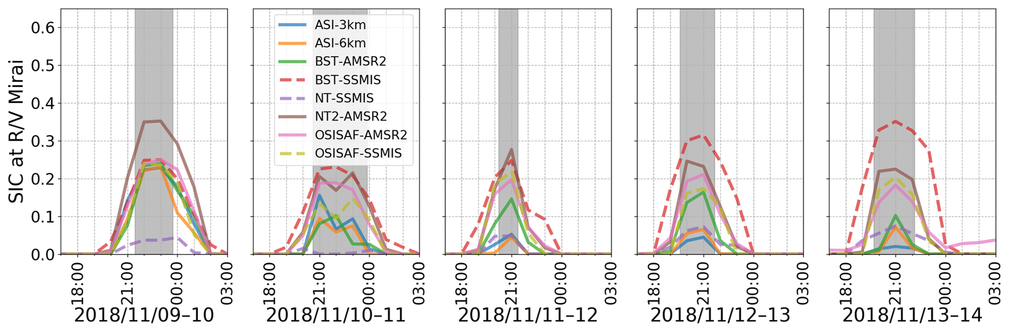
Figure D2Satellite-retrieved SIC for all products along the R/V Mirai track during Phase 1 between 9 and 13 November 2018. The figure schematics of SIC estimates are as follows: ASI-3km (blue), ASI-6km (orange), BST-AMSR2 (green), BST-SSMIS (red), NT2-AMSR2 (purple), NT-SSMIS (brown), OSISAF-AMSR2 (pink), and OSISAF-SSMIS (olive), and SSMIS and AMSR2 are distinguished by dashed and solid lines, respectively. Grey highlighted times indicate when the vessel was in ice cover based on the ice navigator's logs.
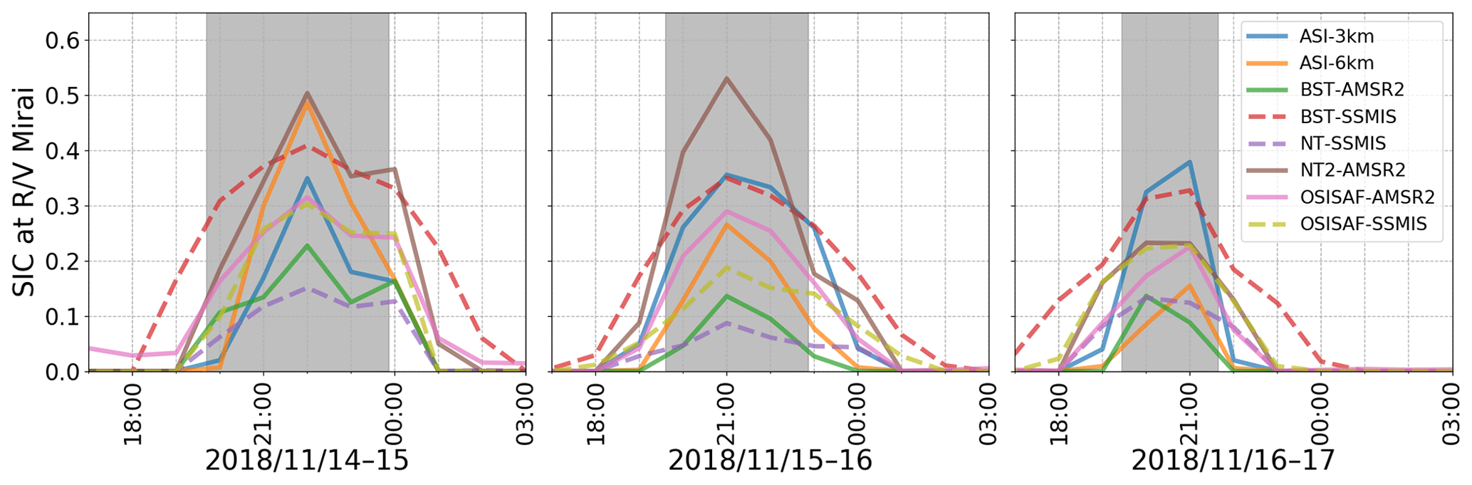
Figure D3Satellite-retrieved SIC for all products along the R/V Mirai track during Phase 2 between 14 and 16 November 2018. The figure schematics follow Fig. D2.
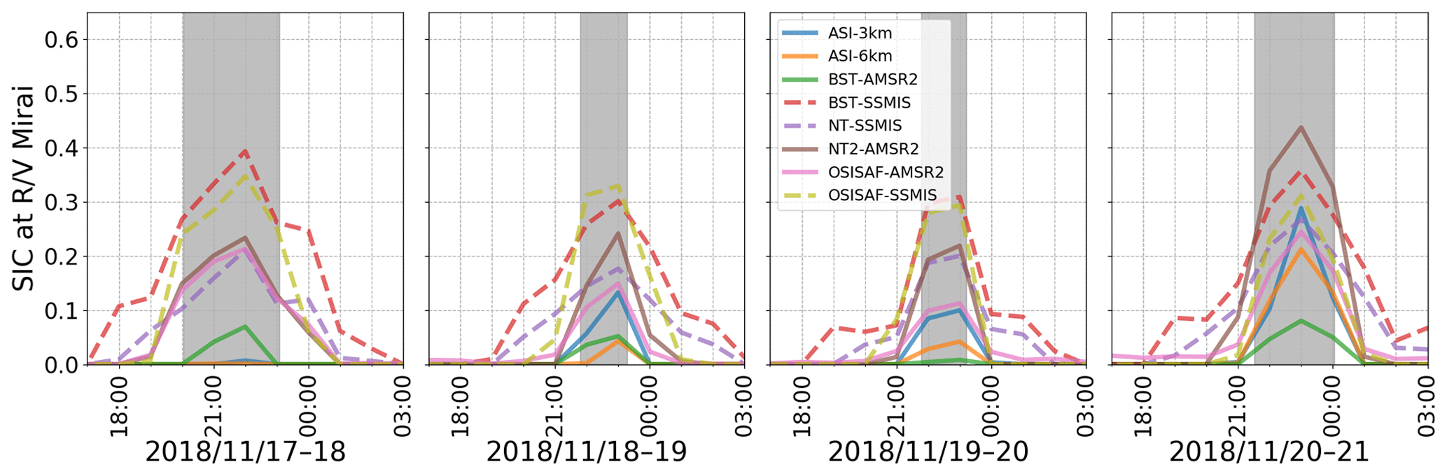
Figure D4Satellite-retrieved SIC for all products along the R/V Mirai track during phases 3 and 4 between 17 and 20 November 2018. The figure schematics follow Fig. D2.
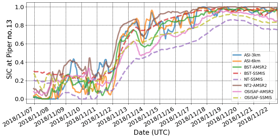
Figure D5Satellite-retrieved SIC for all products along the Piper no. 13 track between 7 and 25 November 2018. The figure schematics of SIC estimates follow Fig. D2.
Figures D2–D4 present the full time series of satellite-retrieved SIC interpolated in time to hourly intervals and bilinearly interpolated in space at the R/V Mirai positions for the MIZ transect sea ice observation period between 9 and 20 November 2018. The figure schematics follow Fig. 2. Lastly, satellite-retrieved SIC data at the Piper no. 13 drifting wave buoy locations also interpolated in time and space are shown in Fig. D5.
Satellite-retrieved SICs were obtained from these sources: Cavalieri et al. (1996–2018), Meier et al. (2018), Comiso (2017–2018), Hori et al. (2012), and Spreen et al. (2008). Furthermore, the OSI-401-b and OSI-408 were used and are the product of the EUMETSAT Ocean and Sea Ice Satellite Application Facility. Sentinel-1 SAR data were downloaded from NOAA (2019), ERA5 data were downloaded from Copernicus (2019), and ARCMFC wave model data were obtained from ARCMFC (2019).
TN formulated the study idea, conducted the analysis, and prepared the manuscript. TW contributed significantly to the analysis and the manuscript. TK and JI continually contributed to the formulation of the manuscript from the start. JI designed the R/V Mirai MIZ transect sea ice observational plan.
The authors declare that they have no conflict of interest.
We sincerely thank Editor David Schroeder for overseeing the peer review process and two anonymous reviewers for the time spent on reviewing this paper and providing valuable and insightful comments that improved the final version.
We are grateful to the R/V Mirai crew on board MR18-05C, who made the MIZ transect sea ice observation possible. Note that our research cruise was supported by the PPP contribution with ECMWF weather and sea ice forecasts and Environment and Climate Change Canada sea ice forecast. The authors greatly appreciate the comprehensive data available freely on the web.
This work was sponsored by the Japanese Ministry of Education, Culture, Sports, Science, and Technology under Arctic Challenge for Sustainability (ArCS, project grant number JPMXD1300000000) and Arctic Challenge for Sustainability II (ArCS II). A part of this study was also conducted under JSPS KAKENHI (grant numbers JP 16H02429 and 19H00801). Jun Inoue received support from the KAKENHI (grant numbers 18H03745 and 18KK0292).
This paper was edited by David Schroeder and reviewed by two anonymous referees.
Andersen, S., Tonboe, R., Kaleschke, L., Heygster, G., and Pedersen, L. T.: Intercomparison of passive microwave sea ice concentration retrievals over the high-concentration Arctic sea ice, J. Geophys. Res.-Oceans, 112, C08004, https://doi.org/10.1029/2006JC003543, 2007. a, b
ARCMFC: ARCMFC wave model data, Index, available at: ftp://nrt.cmems-du.eu/Core/ARCTIC_ANALYSIS_FORECAST_WAV_002_010/dataset-wam-arctic-1hr6km-be/, last access: 11 Augugst, 2019. a, b, c
Ardhuin, F., Rogers, E., Babanin, A. V., Filipot, J.-F., Magne, R., Roland, A., van der Westhuysen, A., Queffeulou, P., Lefevre, J.-M., Aouf, L., and Collard, F.: Semiempirical Dissipation Source Functions for Ocean Waves. Part I: Definition, Calibration, and Validation, J. Phys. Oceanogr., 40, 1917–1941, https://doi.org/10.1175/2010JPO4324.1, 2010. a
Ardhuin, F., Boutin, G., Stopa, J., Girard-Ardhuin, F., Melsheimer, C., Thomson, J., Kohout, A., Doble, M., and Wadhams, P.: Wave attenuation through an Arctic marginal ice zone on October 12, 2015: Part 2. Numerical modeling of waves and associated ice break-up, J. Geophys. Res.-Oceans, 123, 5652–5668, https://doi.org/10.1002/2018JC013784, 2018. a, b, c, d, e, f
Bekkers, E., Francois, J. F., and Rojas-Romagosa, H.: Melting Ice Caps and the Economic Impact of Opening the Northern Sea Route, Econ. J., 128, 1095–1127, https://doi.org/10.1111/ecoj.12460, 2018. a
Boutin, G., Ardhuin, F., Dumont, D., Sevigny, C., Girard-Ardhuin, F., and Accensi, M.: Floe Size Effect on Wave-Ice Interactions: Possible Effects, Implementation in Wave Model, and Evaluation, J. Geophys. Res.-Oceans, 123, 4779–4805, https://doi.org/10.1029/2017JC013622, 2018. a, b, c, d
Boutin, G., Lique, C., Ardhuin, F., Rousset, C., Talandier, C., Accensi, M., and Girard-Ardhuin, F.: Towards a coupled model to investigate wave–sea ice interactions in the Arctic marginal ice zone, The Cryosphere, 14, 709–735, https://doi.org/10.5194/tc-14-709-2020, 2020. a
Canadian Ice Service-Environment Canada: Manual of Ice (MANICE). Manual of Standard Procedures for Observing and Reporting Ice Conditions, Tech. rep., Canadian Ice Service-Environment Canada, Catalogue no. En56-175/2005, 2005. a
Cavalieri, D. J., Gloersen, P., and Campbell, W. J.: Determination of sea ice parameters with the NIMBUS 7 SMMR, J. Geophys. Res.-Atmos., 89, 5355–5369, https://doi.org/10.1029/JD089iD04p05355, 1984. a
Cavalieri, D. J., Parkinson, C. L., Gloersen, P., and Zwally, H. J.: Sea Ice Concentrations from Nimbus-7 SMMR and DMSP SSM/I-SSMIS Passive Microwave Data, Version 1. November 2018, updated yearly, Arctic grid, https://doi.org/10.5067/8GQ8LZQVL0VL, 1996–2018. a, b
Cheng, S., Rogers, W. E., Thomson, J., Smith, M., Doble, M. J., Wadhams, P., Kohout, A. L., Lund, B., Persson, O. P., Collins III, C. O., Ackley, S. F., Montiel, F., and Shen, H. H.: Calibrating a Viscoelastic Sea Ice Model for Wave Propagation in the Arctic Fall Marginal Ice Zone, J. Geophys. Res.-Oceans, 122, 8770–8793, https://doi.org/10.1002/2017JC013275, 2017. a, b, c, d, e
Chevallier, M., Smith, G. C., Dupont, F., Lemieux, J.-F., Forget, G., Fujii, Y., Hernandez, F., Msadek, R., Peterson, K. A., Storto, A., Toyoda, T., Valdivieso, M., Vernieres, G., Zuo, H., Balmaseda, M., Chang, Y.-S., Ferry, N., Garric, G., Haines, K., Keeley, S., Kovach, R. M., Kuragano, T., Masina, S., Tang, Y., Tsujino, H., and Wang, X.: Intercomparison of the Arctic sea ice cover in global ocean–sea ice reanalyses from the ORA-IP project, Clim. Dynam., 49, 1107–1136, https://doi.org/10.1007/s00382-016-2985-y, 2017. a, b
Collins III, C. O., Rogers, W. E., Marchenko, A., and Babanin, A. V.: In situ measurements of an energetic wave event in the Arctic marginal ice zone, Geophys. Res. Lett., 42, 1863–1870, https://doi.org/10.1002/2015gl063063, 2015. a
Comiso, J. C.: Characteristics of Arctic winter sea ice from satellite multispectral microwave observations, J. Geophys. Res.-Oceans, 91, 975–994, https://doi.org/10.1029/JC091iC01p00975, 1986. a
Comiso, J. C.: Enhanced Sea Ice Concentrations from Passive Microwave Data, Tech. rep., NASA Goddard Space Flight Center, available at: https://nsidc.org/sites/nsidc.org/files/files/data/pm/Bootstrap_Algorithm_Revised07.pdf (last access: 30 September 2019), 2007. a, b
Comiso, J. C.: Bootstrap Sea Ice Concentrations from Nimbus-7 SMMR and DMSP SSM/I-SSMIS, Version 3, November 2018, Arctic grid, https://doi.org/10.5067/7Q8HCCWS4I0R, 2017–2018. a, b
Comiso, J. C., Cavalieri, D. J., Parkinson, C. L., and Gloersen, P.: Passive microwave algorithms for sea ice concentration: A comparison of two techniques, Remote Sens. Environ., 60, 357–384, https://doi.org/10.1016/S0034-4257(96)00220-9, 1997. a, b
Comiso, J. C., Meier, W. N., and Gersten, R.: Variability and trends in the Arctic Sea ice cover: Results from different techniques, J. Geophys. Res.-Oceans, 122, 6883–6900, https://doi.org/10.1002/2017JC012768, 2017. a, b, c, d
Copernicus: ERA5 hourly data on single levels from 1979 to present, available at: https://cds.climate.copernicus.eu/cdsapp#!/dataset/reanalysis-era5-single-levels?tab=overview, last access: 11 August 2019. a, b, c
Donlon, C. J., Martin, M., Stark, J., Roberts-Jones, J., Fiedler, E., and Wimmer, W.: The Operational Sea Surface Temperature and Sea Ice Analysis (OSTIA) system, Remote Sens. Environ., 116, 140–158, https://doi.org/10.1016/j.rse.2010.10.017, 2012. a, b
Dumont, D., Kohout, A., and Bertino, L.: A wave-based model for the marginal ice zone including a floe breaking parameterization, J. Geophys. Res.-Oceans, 116, C04001, https://doi.org/10.1029/2010JC006682, 2011. a
Guest, P., Persson, P. O. G., Wang, S., Jordan, M., Jin, Y., Blomquist, B., and Fairall, C.: Low-Level Baroclinic Jets Over the New Arctic Ocean, J. Geophys. Res.-Oceans, 123, 4074–4091, https://doi.org/10.1002/2018JC013778, 2018. a
Heygster, G., Huntemann, M., Ivanova, N., Saldo, R., and Pedersen, L. T.: Response of passive microwave sea ice concentration algorithms to thin ice, in: 2014 IEEE Geoscience and Remote Sensing Symposium, 3618–3621, https://doi.org/10.1109/IGARSS.2014.6947266, 2014. a
Hori, M., Yabuki, H., Sugimura, T., and Terui, T.: AMSR2 Level 3 product of Daily Polar Brightness Temperatures and Product, 1.00, available at: https://ads.nipr.ac.jp/dataset/A20170123-003 (last access: 23 July 2019), 2012. a, b
Inoue, J., Hori, M. E., Enomoto, T., and Kikuchi, T.: Intercomparison of Surface Heat Transfer Near the Arctic Marginal Ice Zone for Multiple Reanalyses: A Case Study of September 2009, SOLA, 7, 57–60, https://doi.org/10.2151/sola.2011-015, 2011. a
Ivanova, N., Pedersen, L. T., Tonboe, R. T., Kern, S., Heygster, G., Lavergne, T., Sørensen, A., Saldo, R., Dybkjær, G., Brucker, L., and Shokr, M.: Inter-comparison and evaluation of sea ice algorithms: towards further identification of challenges and optimal approach using passive microwave observations, The Cryosphere, 9, 1797–1817, https://doi.org/10.5194/tc-9-1797-2015, 2015. a, b, c, d
Jakobsson, M., Mayer, L., Coakley, B., Dowdeswell, J. A., Forbes, S., Fridman, B., Hodnesdal, H., Noormets, R., Pedersen, R., Rebesco, M., Schenke, H. W., Zarayskaya, Y., Accettella, D., Armstrong, A., Anderson, R. M., Bienhoff, P., Camerlenghi, A., Church, I., Edwards, M., Gardner, J. V., Hall, J. K., Hell, B., Hestvik, O., Kristoffersen, Y., Marcussen, C., Mohammad, R., Mosher, D., Nghiem, S. V., Pedrosa, M. T., Travaglini, P. G., and Weatherall, P.: The International Bathymetric Chart of the Arctic Ocean (IBCAO) Version 3.0, Geophys. Res. Lett., 39, L12609, https://doi.org/10.1029/2012GL052219, 2012. a
JAMSTEC: R/V Mirai Cruise Report MR18-05C Arctic Challenge and for Sustainability (ArCS), Arctic Ocean, Bering Sea, and North Pacific, 24 October–7 December2018, Tech. rep., Japan Agency for Marine-Earth Science and Technology (JAMSTEC), available at: http://www.godac.jamstec.go.jp/catalog/data/doc_catalog/media/MR18-05C_all.pdf (last access: 7 August 2019), 2018. a
JAMSTEC: Oceanographic Research Vessel MIRAI, available at: https://www.jamstec.go.jp/e/about/equipment/ships/mirai.html, last access: 22 July 2019. a
Jung, T., Gordon, N. D., Bauer, P., Bromwich, D. H., Chevallier, M., Day, J. J., Dawson, J., Doblas-Reyes, F., Fairall, C., Goessling, H. F., Holland, M., Inoue, J., Iversen, T., Klebe, S., Lemke, P., Losch, M., Makshtas, A., Mills, B., Nurmi, P., Perovich, D., Reid, P., Renfrew, I. A., Smith, G., Svensson, G., Tolstykh, M., and Yang, Q.: Advancing Polar Prediction Capabilities on Daily to Seasonal Time Scales, B. Am. Meteorol. Soc., 97, 1631–1647, https://doi.org/10.1175/BAMS-D-14-00246.1, 2016. a
Kodaira, T., Waseda, T., Nose, T., Sato, K., Inoue, J., Voermans, J., and Babanin, A.: Observation of on-ice wind waves under grease ice in the western Arctic Ocean, Polar Science, in review, 2020. a
Kohout, A. L., Williams, M. J. M., Dean, S. M., and Meylan, M. H.: Storm-induced sea-ice breakup and the implications for ice extent, Nature, 509, 604–607, https://doi.org/10.1038/nature13262, 2014. a
Kohout, A. L., Penrose, B., Penrose, S., and Williams, M. J.: A device for measuring wave-induced motion of ice floes in the Antarctic Marginal Ice Zone, Ann. Glaciol., 56, 415–424, https://doi.org/10.3189/2015aog69a600, 2015. a, b
Kwok, R. and Rothrock, D. A.: Decline in Arctic sea ice thickness from submarine and ICESat records: 1958–2008, Geophys. Res. Lett., 36, L15501, https://doi.org/10.1029/2009GL039035, 2009. a
Lavergne, T., Sørensen, A. M., Kern, S., Tonboe, R., Notz, D., Aaboe, S., Bell, L., Dybkjær, G., Eastwood, S., Gabarro, C., Heygster, G., Killie, M. A., Brandt Kreiner, M., Lavelle, J., Saldo, R., Sandven, S., and Pedersen, L. T.: Version 2 of the EUMETSAT OSI SAF and ESA CCI sea-ice concentration climate data records, The Cryosphere, 13, 49–78, https://doi.org/10.5194/tc-13-49-2019, 2019. a, b
Li, J., Kohout, A. L., Doble, M. J., Wadhams, P., Guan, C., and Shen, H. H.: Rollover of Apparent Wave Attenuation in Ice Covered Seas, J. Geophys. Res.-Oceans, 122, 8557–8566, https://doi.org/10.1002/2017JC012978, 2017. a
Liu, A. K. and Mollo-Christensen, E.: Wave Propagation in a Solid Ice Pack, J. Phys. Oceanogr., 18, 1702–1712, https://doi.org/10.1175/1520-0485(1988)018<1702:WPIASI>2.0.CO;2, 1988. a, b, c
Liu, Q., Rogers, W. E., Babanin, A. V., Young, I. R., Romero, L., Zieger, S., Qiao, F., and Guan, C.: Observation-Based Source Terms in the Third-Generation Wave Model WAVEWATCH III: Updates and Verification, J. Phys. Oceanogr., 49, 489–517, https://doi.org/10.1175/JPO-D-18-0137.1, 2019. a
Maslanik, J. A., Fowler, C., Stroeve, J., Drobot, S., Zwally, J., Yi, D., and Emery, W.: A younger, thinner Arctic ice cover: Increased potential for rapid extensive sea-ice loss, Geophys. Res. Lett., 34, L24501, https://doi.org/10.1029/2007GL032043, 2007. a
Meier, W. N.: Comparison of passive microwave ice concentration algorithm retrievals with AVHRR imagery in Arctic peripheral seas, IEEE T. Geosci. Remote, 43, 1324–1337, https://doi.org/10.1109/TGRS.2005.846151, 2005. a, b
Meier, W. N., Markus, T., and Comiso, J. C.: AMSR-E/AMSR2 Unified L3 Daily 12.5 km Brightness Temperatures, Sea Ice Concentration, Motion & Snow Depth Polar Grids, Version 1, November 2018, Arctic grid, https://doi.org/10.5067/RA1MIJOYPK3P, 2018. a, b
Meylan, M. H. and Masson, D.: A linear Boltzmann equation to model wave scattering in the marginal ice zone, Ocean Model., 11, 417–427, https://doi.org/10.1016/j.ocemod.2004.12.008, 2006. a
Montiel, F., Squire, V. A., Doble, M., Thomson, J., and Wadhams, P.: Attenuation and Directional Spreading of Ocean Waves During a Storm Event in the Autumn Beaufort Sea Marginal Ice Zone, J. Geophys. Res.-Oceans, 123, 5912–5932, https://doi.org/10.1029/2018JC013763, 2018. a
Mosig, J. E. M., Montiel, F., and Squire, V. A.: Comparison of viscoelastic-type models for ocean wave attenuation in ice-covered seas, J. Geophys. Res.-Oceans, 120, 6072–6090, https://doi.org/10.1002/2015JC010881, 2015. a, b, c, d
NOAA: Sentinel-1 SAR data, Index, available at: ftp://ftpcoastwatch.noaa.gov/pub/socd6/coastwatch/s1/sar/nrcs/2018/, last access: 10 August 2019. a, b, c, d
Nose, T., Webb, A., Waseda, T., Inoue, J., and Sato, K.: Predictability of storm wave heights in the ice-free Beaufort Sea, Ocean Dynam. 68, 1383–1402, https://doi.org/10.1007/s10236-018-1194-0, 2018. a, b, c
Notz, D.: Sea-ice extent and its trend provide limited metrics of model performance, The Cryosphere, 8, 229–243, https://doi.org/10.5194/tc-8-229-2014, 2014. a, b, c
Rascle, N. and Ardhuin, F.: A global wave parameter database for geophysical applications. Part 2: Model validation with improved source term parameterization, Ocean Model., 70, 174 –188, https://doi.org/10.1016/j.ocemod.2012.12.001, 2013. a
Roach, L. A., Dean, S. M., and Renwick, J. A.: Consistent biases in Antarctic sea ice concentration simulated by climate models, The Cryosphere, 12, 365–383, https://doi.org/10.5194/tc-12-365-2018, 2018. a, b
Roach, L. A., Bitz, C. M., Horvat, C., and Dean, S. M.: Advances in Modeling Interactions Between Sea Ice and Ocean Surface Waves, J. Adv. Model. Earth Sy., 11, 4167–4181, https://doi.org/10.1029/2019MS001836, 2019. a
Rogers, W. E. and Campbell, T. J.: Implementation of curvilinear coordinate system in the WAVEWATCH III model, Tech. Rep. NRL/MR/7320–09-9193, Naval Research Laboratory, Stennis Space Center, 2009. a
Rogers, W. E., Babanin, A. V., and Wang, D. W.: Observation-Consistent Input and Whitecapping Dissipation in a Model for Wind-Generated Surface Waves: Description and Simple Calculations, J. Atmos. Ocean. Tech., 29, 1329–1346, https://doi.org/10.1175/JTECH-D-11-00092.1, 2012. a
Rogers, W. E., Thomson, J., Shen, H. H., Doble, M. J., Wadhams, P., and Cheng, S.: Dissipation of wind waves by pancake and frazil ice in the autumn Beaufort Sea, J. Geophys. Res.-Oceans, 121, 7991–8007, https://doi.org/10.1002/2016jc012251, 2016. a, b, c, d, e, f
Spreen, G., Kaleschke, L., and Heygster, G.: Sea ice remote sensing using AMSR-E 89-GHz channels, J. Geophys. Res.-Oceans, 113, C02S03, https://doi.org/10.1029/2005JC003384, 2008. a, b, c, d
Squire, V. A.: Of ocean waves and sea-ice revisited, Cold Reg. Sci. Technol., 49, 110–133, https://doi.org/10.1016/j.coldregions.2007.04.007, 2007. a
Squire, V. A.: A fresh look at how ocean waves and sea ice interact, Philos. T. R. Soc. A, 376, 20170342, https://doi.org/10.1098/rsta.2017.0342, 2018. a, b
Stephenson, S. R., Smith, L. C., Brigham, L. W., and Agnew, J. A.: Projected 21st-century changes to Arctic marine access, Clim. Change, 118, 885–899, https://doi.org/10.1007/s10584-012-0685-0, 2013. a
Stroeve, J. and Notz, D.: Changing state of Arctic sea ice across all seasons, Environ. Res. Lett., 13, 103001, https://doi.org/10.1088/1748-9326/aade56, 2018. a
Stroeve, J. C., Serreze, M. C., Holland, M. M., Kay, J. E., Malanik, J., and Barrett, A. P.: The Arctic's rapidly shrinking sea ice cover: a research synthesis, Clim. Change, 110, 1005–1027, https://doi.org/10.1007/s10584-011-0101-1, 2012. a
Sutherland, G., Rabault, J., Christensen, K. H., and Jensen, A.: A two layer model for wave dissipation in sea ice, Appl. Ocean Res., 88, 111–118, https://doi.org/10.1016/j.apor.2019.03.023, 2019. a, b
The WAVEWATCH III® Development Group (WW3DG): User manual and system documentation of WAVEWATCH III® version 6.07, Tech. Note 333, NOAA/NWS/NCEP/MMAB, College Park, MD, USA, 465 pp., 2019. a
Thomson, J., Ackley, S., Girard-Ardhuin, F., Ardhuin, F., Babanin, A., Boutin, G., Brozena, J., Cheng, S., Collins, C., Doble, M., Fairall, C., Guest, P., Gebhardt, C., Gemmrich, J., Graber, H. C., Holt, B., Lehner, S., Lund, B., Meylan, M. H., Maksym, T., Montiel, F., Perrie, W., Persson, O., Rainville, L., Erick Rogers, W., Shen, H., Shen, H., Squire, V., Stammerjohn, S., Stopa, J., Smith, M. M., Sutherland, P., and Wadhams, P.: Overview of the Arctic Sea State and Boundary Layer Physics Program, J. Geophys. Res.-Oceans, 123, 8674–8687, https://doi.org/10.1002/2018JC013766, 2018. a, b, c, d
TSK Tsurumi Seiki Co. Ltd.: Oceanographic Equipment Water Quality Monitoring Equipment | TSK Tsurumi Seiki Co., Ltd. – Microwave Type Wave Height Meter WM-2, available at: http://www.tsk-jp.com/index.php?page=/product/detail/21/2, last access: 23 July 2019. a, b, c
Virtanen, P., Gommers, R., Oliphant, T. E., Haberland, M., Reddy, T., Cournapeau, D., Burovski, E., Peterson, P., Weckesser, W., Bright, J., van der Walt, S. J., Brett, M., Wilson, J., Millman, J. K., Mayorov, N., Nelson, A. R. J., Jones, E., Kern, R., Larson, E., Carey, C. J., Polat, İ., Feng, Y., Moore, E. W., Vand erPlas, J., Laxalde, D., Perktold, J., Cimrman, R., Henriksen, I., Quintero, E. A., Harris, C. R., Archibald, A. M., Ribeiro, A. H., Pedregosa, F., van Mulbregt, P., and SciPy 1.0 Contributors: SciPy: SciPy 1.0: Fundamental Algorithms for Scientific Computing in Python, Nat. Methods, 17, 261–272, https://doi.org/10.1038/s41592-019-0686-2, 2020. a
Wang, R. and Shen, H. H.: Gravity waves propagating into an ice-covered ocean: A viscoelastic model, J. Geophys. Res.-Oceans, 115, C06024, https://doi.org/10.1029/2009JC005591, 2010. a, b, c
Wessel, P. and Smith, W. H. F.: A global, self-consistent, hierarchical, high-resolution shoreline database, J. Geophys. Res.-Sol. Ea., 101, 8741–8743, https://doi.org/10.1029/96JB00104, 1996. a
Williams, T. D., Bennetts, L. G., Squire, V. A., Dumont, D., and Bertino, L.: Wave–ice interactions in the marginal ice zone. Part 1: Theoretical foundations, Ocean Model., 71, 81–91, https://doi.org/10.1016/j.ocemod.2013.05.010, 2013. a
WMO: WMO Sea-Ice Nomenclature, Tech. Rep. 259, The Joint Technical Commission for Oceanography and Marine Meteorology (JCOMM), available at: https://www.jcomm.info/index.php?option=com_oe&task=viewDocumentRecord&docID=14598 (last access: 22 January 2020), 2014. a, b
Zhang, Y., Chen, C., Beardsley, R. C., Perrie, W., Gao, G., Zhang, Y., Qi, J., and Lin, H.: Applications of an unstructured grid surface wave model (FVCOM-SWAVE) to the Arctic Ocean: The interaction between ocean waves and sea ice, Ocean Model., 145, 101532, https://doi.org/10.1016/j.ocemod.2019.101532, 2020. a
Zieger, S., Babanin, A. V., Rogers, W. E., and Young, I. R.: Observation-based source terms in the third-generation wave model WAVEWATCH, Ocean Model., 96, 2–25, https://doi.org/10.1016/j.ocemod.2015.07.014, 2015. a
As documented in https://resources.marine.copernicus.eu/documents/PUM/CMEMS-ARC-PUM-WAV-002-014.pdf (last access: 10 April 2020).
- Abstract
- Introduction
- Methods
- Sea ice concentration: definition, characteristics, and use in wave–ice models
- Δci effects on wave modelling at the observation sites
- Δci and wave modelling in the refreezing Chukchi Sea
- Conclusions and discussions
- Appendix A: R/V Mirai measurement system
- Appendix B: Supplementary information of TodaiWW3-ArCS and the dispersion relation of WAVEWATCH III ® wave–ice interaction models
- Appendix C: OSISAF-AMSR2 noise in open ocean
- Appendix D: R/V Mirai MIZ transect sea ice observation and satellite-retrieved SIC at the observation locations
- Data availability
- Author contributions
- Competing interests
- Acknowledgements
- Financial support
- Review statement
- References