the Creative Commons Attribution 4.0 License.
the Creative Commons Attribution 4.0 License.
 | 24 Jun 2020
Glacier runoff variations since 1955 in the Maipo River basin, in the semiarid Andes of central Chile
David Farías-Barahona
Matthias Huss
Francesca Pellicciotti
James McPhee
Daniel Farinotti
As glaciers adjust their size in response to climate variations, long-term changes in meltwater production can be expected, affecting the local availability of water resources. We investigate glacier runoff in the period 1955–2016 in the Maipo River basin (4843 km2, 33.0–34.3∘ S, 69.8–70.5∘ W), in the semiarid Andes of Chile. The basin contains more than 800 glaciers, which cover 378 km2 in total (inventoried in 2000). We model the mass balance and runoff contribution of 26 glaciers with the physically oriented and fully distributed TOPKAPI (Topographic Kinematic Approximation and Integration)-ETH glacio-hydrological model and extrapolate the results to the entire basin. TOPKAPI-ETH is run at a daily time step using several glaciological and meteorological datasets, and its results are evaluated against streamflow records, remotely sensed snow cover, and geodetic mass balances for the periods 1955–2000 and 2000–2013. Results show that in 1955–2016 glacier mass balance had a general decreasing trend as a basin average but also had differences between the main sub-catchments. Glacier volume decreased by one-fifth (from 18.6±4.5 to 14.9±2.9 km3). Runoff from the initially glacierized areas was 177±25 mm yr−1 (16±7 % of the total contributions to the basin), but it shows a decreasing sequence of maxima, which can be linked to the interplay between a decrease in precipitation since the 1980s and the reduction of ice melt. Glaciers in the Maipo River basin will continue retreating because they are not in equilibrium with the current climate. In a hypothetical constant climate scenario, glacier volume would reduce to 81±38 % of the year 2000 volume, and glacier runoff would be 78±30 % of the 1955–2016 average. This would considerably decrease the drought mitigation capacity of the basin.
- Article
(5728 KB) - Full-text XML
-
Supplement
(1659 KB) - BibTeX
- EndNote


Most glaciers on Earth have retreated due to global atmospheric warming during the 20th century (Zemp et al., 2019). Glaciers that are still out of balance with the present climate are committed to lose part of their mass in the coming decades, even without further warming (Zemp et al., 2015; Marzeion et al., 2018), and major changes in their meltwater production can be anticipated (Bliss et al., 2014; Huss and Hock, 2018; IPCC, 2020). In the absence of precipitation changes, a temporary increase in meltwater generation from a retreating glacier occurs as a consequence of higher air temperatures and enhanced ablation, but after this transient phase melt amounts decrease due to the reduction of the available snow, firn and ice volumes (Jansson et al., 2003). The period in which the annual melt volume reaches its long-term maximum has been termed “peak water” (Gleick and Palaniappan, 2010; Baraer et al., 2012). Global-scale studies indicate a large heterogeneity in the geographical distribution of peak water, while several catchments in the Himalayas and Alaska are expected to increase their glacier runoff due to the enhanced ablation in the next decades and reach a maximum at some point of the 21st century, other regions in the world, such as the semiarid Andes, central Europe, and western Canada, have already reached a regional maximum, and thus glacier runoff will only decrease in the future (Bliss et al., 2014; Huss and Hock, 2018). While these studies provide global trends that are key for macro-regional assessments, studies focusing on the catchment scale can provide more specific information about local hydro-glaciological changes to communities and stakeholders for the generation of mitigation and adaptation strategies. Additionally, catchment-scale studies place glacier runoff in the context of other components of the water cycle and evaluate the impacts of glacier changes on downstream areas.
In this study, we focus on glacier changes and their impacts on long-term glacier runoff contribution in the semiarid Andes. Meltwater originating in the Andes is key for Chile and the western areas of Argentina, as it represents the main source of water for drinking water, agriculture, industry, mining, and natural ecosystems. The climate of this region is characterized by its strong interannual variability of precipitation linked to periodic atmosphere–ocean variations over the Pacific Ocean (Montecinos and Aceituno, 2003; Falvey and Garreaud, 2007) and a sustained air temperature increase during the last decades (Carrasco et al., 2005; Burger et al., 2018). A few studies have estimated the present (Ragettli and Pellicciotti, 2012; Ayala et al., 2016; Burger et al., 2019) and future (Ragettli et al., 2016; Huss and Hock, 2018) glacier runoff contribution in the semiarid Andes, but its past variations have not been analyzed in detail, mostly due to the lack of long-term glaciological data. As future climate scenarios anticipate a decrease in glacier runoff (e.g., Ragettli et al., 2016), the question of whether peak water has already occurred still remains open. The assessment of long-term changes in glacier runoff is particularly useful for water planners because it provides reference information for the role of glacier meltwater in river flows, and the impacts that can be anticipated in the absence of its contribution.
Glaciers in the semiarid Andes underwent a major retreat in the 20th century (Le Quesne et al., 2009; Malmros et al., 2016) and the last 2 decades (Braun et al., 2019; Dussaillant et al., 2019). Historical documents, aerial photographs, and dendrochronological studies suggest that the general retreat trend started around the mid-19th century, but it has been interrupted by occasional periods of positive mass balance accompanied by glacier advances (Le Quesne et al., 2009; Masiokas et al., 2009). Masiokas et al. (2016) performed a reconstruction of the annual mass balance of Echaurren Norte Glacier (3650–3900 m a.s.l.) since 1909 using a simple glacier mass balance model forced with monthly precipitation and air temperature. The model was verified against streamflow records and direct mass balance measurements on the glacier, where the first mass balance monitoring program in the southern Andes started in 1975. Masiokas et al. (2016) found a general retreat interrupted by three periods of sustained positive mass balance in the 1920–1930s, 1980s, and 2000s. The latter positive or balanced mass budget in the semiarid Andes in the 2000–2009 period has been recently verified by geodetic mass balances (Braun et al., 2019; Dussaillant et al., 2019; Farías-Barahona et al., 2019) and has been supported by independent modeling results (Burger et al., 2019). As the findings by Masiokas et al. (2016) are based on a relatively simple model applied to only one glacier at low elevation (<4000 m a.s.l.), they cannot be extrapolated to other glaciers. This is especially true due to the large spatial variability of response times and retreat rates reported for this region (Malmros et al., 2016). Thus, a more detailed analysis based on the specific characteristics of each glacier is needed to complement these results and estimate regional changes of ice volume and glacier runoff. From a climatic perspective, glacier retreat in the semiarid Andes has been driven by a general temperature increase and modulated by a strong temporal variability of precipitation. Air temperature showed an increasing trend of about 0.25 ∘C per decade in the period 1979–2006 (Falvey and Garreaud, 2009), mostly explained by a spring and autumn warming (Burger et al., 2018), which can be used to explain an increase in the 0 ∘C isotherm and the regional equilibrium line altitude (ELA) (Carrasco et al., 2005, 2008). Precipitation, on the other hand, exhibited an average decrease of −65 mm (−7.1 %) per decade in the period 1979–2016 (Boisier et al., 2016), although it has a large interannual and inter-decadal variability (Montecinos and Aceituno, 2003).
Our main objectives are to reconstruct glacier changes (area and volume) during the last 6 decades in one of the main catchments of the semiarid Andes, the Maipo River basin; analyze the role of glaciers in the regional hydrology; and identify the main trends in glacier runoff. Glacier runoff is defined as the water originating from ice melt, snowmelt and rain over a given glacier. Additionally, we estimate glacier changes under synthetic scenarios of committed ice loss, in which air temperature, precipitation and cloudiness are assumed to stay at their current levels until the end of the century. We use these scenarios for (i) understanding how far the glaciers are from an equilibrium after the climatic changes that took place in the period 1955–2016 and (ii) providing a baseline for the future changes in hydrology that the basin will experience in any case, i.e., even in the hypothetical case that climate change was to stall. The scenarios are thus highly conservative and do not correspond to a realistic projection for the future. The calculation of glacier changes and runoff contribution is carried out for a subset of the largest glaciers using the physically oriented and fully distributed TOPKAPI-ETH glacio-hydrological model (Fatichi et al., 2014; Ragettli et al., 2016), and the resulting mass balances are extrapolated to the entire basin (Huss, 2012). We set up the glacier model using glacier inventories, digital elevation models (DEMs), and estimates of ice thickness, and we force it with a combination of local meteorological stations and reanalysis data for precipitation, air temperature, and solar radiation. The model is calibrated and validated using remotely sensed snow cover, streamflow records, and geodetic mass balances covering the periods 1955–2000 and 2000–2013 (Braun et al., 2019; Farías-Barahona et al., 2020).
The study focuses on the headwaters of the Maipo River basin (hereafter we refer to these areas as the Maipo River basin for simplicity). The basin is located in central Chile (∼33∘ S, ∼70∘ W), to the east of the Chilean capital city, Santiago (Fig. 1a), to which it provides about 70 % of its drinking water (DGA, 2004). The basin outlet is the Maipo en El Manzano gauging station, which roughly marks the boundary between rural mountain areas and Santiago urban districts. The selected basin has an area of 4843 km2, its elevation ranges from 850 to 6570 m a.s.l., and more than 800 glaciers covering about 378 km2 (7.8 % glacierized) were inventoried in 2000 (Barcaza et al., 2017). The Maipo River and its tributaries are the primary source for drinking water, agriculture, hydropower, and industry in the region, which concentrates about 40 % of the country's population. The region has a Mediterranean-type climate, with a strong seasonality characterized by cold and wet winters and hot and dry summers. Average precipitation in Santiago was 308 mm yr−1 in the period 1950–2018, but values as low as 69 mm yr−1 and as high as 712 mm yr−1 have been registered, with a coefficient of variation of 0.45. Recurrent droughts have been reported since the beginning of hydrometeorological records. Precipitation amounts are, in general, larger towards the south and towards higher elevations. An early study estimated that glacier runoff in the Maipo River basin represents about 34 % of the total discharge in February and up to 67 % during summer months of dry years, such as 1968–1969 (Peña and Nazarala, 1987).

Figure 1(a) Maipo River basin, next to the city of Santiago in central Chile. (b) The basin outlet and the sub-catchments, rivers, main glaciers, and hydrometeorological stations. (c) The elevation range of every glacier in the basin as a function of the average latitude (arbitrary scale) in each sub-catchment and the mean elevation (black line). (d) Estimated total ice volume using the method developed by Huss and Farinotti (2012) (left axis) and glacierized area (right axis) in each sub-catchment. The surface and glacier type (debris-free, debris-covered, or rock glacier) and the number of glaciers in each sub-catchment are indicated.
There are five major sub-catchments in the study area, from north to south: Olivares, Colorado, Yeso, Volcán, and Upper Maipo (Fig. 1b). According to the national Chilean inventory (Barcaza et al., 2017) (described in the next section), the highest glacierized sites are in the Olivares and Colorado sub-catchments, with mean elevations between 4200 and 4500 m a.s.l., and some glaciers reaching elevations higher than 5500 m a.s.l. (Fig. 1c). The Upper Maipo sub-catchment, on the other hand, has the lowest-lying glaciers, with mean elevation varying between 3500 and 4000 m a.s.l., and several glaciers reaching elevations below 3000 m a.s.l. (Fig. 1c). Glacierized areas vary from 40 km2 in the Volcán sub-catchment to 99 km2 in Colorado. Upper Maipo has the largest number of individual glaciers (348), and most of them correspond to low-elevation, rock, and debris-covered glaciers (Fig. 1d). In general, glacier size tends to decrease towards the south, with the largest glaciers being located in Olivares (Juncal Sur, Olivares Gama, and Olivares Beta glaciers) and on the slopes of Tupungatito and Marmolejo volcanoes (Volcán Tupungatito, Azufre, and Marmolejo glaciers) in the Colorado sub-catchment. Another series of relatively large glaciers corresponds to debris-covered ones, such as Pirámide, Loma Larga, and Cerro Castillo glaciers.
3.1 Geographic and topographic information
Glacier outlines are extracted from the national Chilean inventory (Barcaza et al., 2017) and the Marangunic inventory (Marangunic, 1979). While the information for the Maipo River basin in the national inventory was produced using two satellite images from the Landsat Enhanced Thematic Mapper ETM+ of 2003, the Marangunic inventory was mostly based on aerial photographs taken in 1955 during a national geodetic program and maps presented by Lliboutry (1956) for the few missing areas. For consistency with the DEM obtained from the Shuttle Radar Topography Mission (SRTM), we assume that the outlines in the national inventory from 2003 are also valid for 2000. Additionally, the glacierized areas in the national inventory that are not identified as such in 1955 (mostly rock glaciers and debris-covered areas) are added to the 1955 inventory. In this study, we assign an error of 5 % to the year 2000 inventory, which is a common choice for glacier inventories (Paul et al., 2013), and has been used for this inventory in particular (Barcaza et al., 2017). As the inventory of 1955 suffers from additional errors (such as the presence of snow patches that likely made the interpretation of glacierets difficult, and the use of Lliboutry maps to fill missing areas), we assume an error of 10 % for that year. Based on the resulting inventories, we estimate that the total glacier area changed from 532 km2 in 1955 to 378 km2 in 2000 (−28.9 %) and that the number of individual glaciers decreased from 861 to 854. Although some small glaciers might have effectively disappeared, the decreasing trend in the total number of glaciers is also balanced by the fragmentation of large glaciers, such as the Olivares Alfa glacier complex, into several smaller units (Malmros et al., 2016).
In addition to the glacier inventory, we generate a mask of debris-covered glacier areas from the same Landsat images that were used to produce the Chilean glacier inventory. For this, we use the semiautomatic method based on band ratio segmentation of TM4 and TM5 Landsat bands (Paul et al., 2004), and we manually correct the results using Google Earth imagery. For the year 1955, we maintain the same debris cover maps as in the 2000–2010 period, i.e., assuming that no major changes have occurred in the extension of debris cover, but we delete small debris-covered areas on the upper glacier areas.
In our analyses, we use the DEMs for the years 1955, 2000, and 2013 and the geodetic mass balance datasets for the periods 1955–2000 and 2000–2013, as calculated by Farías-Barahona et al. (2020) and Braun et al. (2019). While the DEMs for 2000 and 2013 correspond to a part of the products generated in the study of Braun et al. (2019) for the entire South American Andes, the DEM for 1955 and the geodetic mass balance for the period 1955–2000 were produced in the study of Farías-Barahona et al. (2020), who extended the period of analysis of Braun et al. (2019) for the Maipo River basin. Here, we provide a brief description of the derivation of these datasets, but more details are included in the Supplement. The 1955 DEM was calculated from digitized 50 m contour lines of the 1:50 000 official Chilean cartography product, which was also obtained from the 1955 geodetic program. While the DEMs for the year 2000 were extracted from the SRTM product, the DEM of Maipo River basin for 2013 was derived from TanDEM-X post-processed products (which for this region correspond to the year 2013). The DEMs were co-registered following Nuth and Kääb (2011). Errors from the geodetic mass balances were assessed over stable ground, and calculated using a standard error propagation procedure, including typical error sources such as radar penetration signal. Two glaciers (San Francisco and Mirador del Morado) were discarded from the geodetic mass balance because the original SRTM product was not available for those areas (only the void-filled product). As rock glaciers exhibit changes that are smaller than the estimated uncertainties, they were also discarded from the geodetic mass balance.
3.2 Ice thickness
Distributed glacier ice thickness in 2000 is estimated for all individual glaciers using the method of Huss and Farinotti (2012) with the glacier outlines and the SRTM DEM. Standard model parameters are used except for glaciers classified as debris-covered or rock glaciers. For these two types of ice bodies, the parameter prescribing ice flux is substantially reduced to obtain thicknesses comparable to the direct thickness observations on the debris-covered Pirámide Glacier and its neighboring rock glaciers (DGA, 2012). The obtained ice thickness estimates compare well with ground-penetrating radar (GPR) measurements (DGA, 2014) on Volcán Tupungatito (1685 data points) and Marmolejo (1544 data points) glaciers extracted from the Glacier Thickness Database (GlaThiDa) (Gärtner-Roer et al., 2014), for which we find a root-mean-square error (RMSE) of 9.8 and 8.5 m, respectively.
Once the distributed ice thickness is calculated for every glacier for the year 2000, we use the geodetic mass balance in the period 1955–2000 to estimate the ice thickness distribution in 1955. In this procedure, we find the problem that for some grid cells showing a positive elevation change from the geodetic mass balance for the 1955–2000 period, the ice thickness in year 2000 is too small, resulting in an inferred negative thickness. To avoid this and obtain meaningful 1955 ice thicknesses that are consistent with both the geodetic mass balance and the glacier inventory, we assign the year 2000 ice thickness to 1955 in these grid cells and add the estimated positive elevation change. In this way, we obtain a corrected ice thickness value in 2000 for 4.8 % of the glacierized area. As no geodetic mass balance was calculated for rock glaciers, they are assumed to have the same thickness in 1955 as in year 2000. A similar result was found in the study of Bodin et al. (2010) for rock glaciers near Santiago. Finally, to calculate the 1955 ice thickness of small glaciers that are not included in the year 2000 inventory, we use the 1955 glacier areas from the glacier inventory and a scaling relation to calculate mean ice thickness () as a function of the glacier area (S) and assume average thickness to be valid for every grid cell in these glaciers:
where γ=1.357 and c=28.5 are standard parameters in the volume–area scaling relation (Chen and Ohmura, 1990).
At the basin scale, we find a total ice volume of 18.6±4.1 km3 and 16.1±2.4 km3 for 1955 and 2000 (a change of −13.8 %), respectively. Based on the geodetic mass balances for the period 2000–2013, we estimate a total ice volume of 15.2±3.2 km3 for the year 2013 (a change of −18.4 % relative to 1955). For the total ice volume of the investigated basin, we assume an uncertainty of 15 % in year 2000. This is between the values estimated by Huss and Farinotti (2012) for regional totals (∼12 %) and the value estimated by Farinotti et al. (2017) for individual glaciers (∼21 %). The uncertainty in the total ice volume in 1955 and 2013 is larger than in 2000 since it also includes the uncertainty from the geodetic mass balances. In the calculation of glacier volumes, we implicitly assume that no basal melting takes place. The error introduced by neglecting this process is much less than the uncertainty associated with the ice thickness estimates and the geodetic mass balance.
3.3 Hydrometeorological data
Precipitation and temperature data for the period 1979–2016 are derived from daily gridded products developed by the Centre for Climate and Resilience Research in Santiago, Chile (CR2, http://www.cr2.cl, last access: 19 August 2019). These products were generated for a national water balance study led by the Chilean directorate of water resources (DGA) (DGA, 2017; Álvarez-Garretón et al., 2018). The CR2 daily precipitation product was generated by means of a statistical downscaling of precipitation and moisture fluxes from the ERA-Interim reanalysis. The downscaling procedure is based on multiple linear regressions with topographic parameters, which were calibrated with quality-controlled precipitation records. The CR2 temperature product was obtained using near-surface temperature from ERA-Interim and land surface temperature (LST) from the Moderate Resolution Imaging Spectroradiometer (MODIS), by means of multiple regression models using LST as the explanatory variable and validated with local observations. For our study, while the CR2 precipitation product is linearly interpolated from its original resolution (0.05∘) to the spatial resolutions of our glacio-hydrological models (1 km and 100 m; see Sect. 4.1.2 and 4.1.3) to generate monthly average maps, the CR2 temperature product is used to generate basin-scale daily temperature lapse rates.
Daily cloud transmissivity of solar radiation is calculated from the Chilean solar radiation database (http://www.minenergia.cl/exploradorsolar/, last access: 19 August 2019) for the period 2004–2016 at the location of Embalse El Yeso meteorological station, which is placed close to the centroid of the Maipo River basin, and assumed to be uniform over the catchment. The solar radiation database was derived using reanalysis data to force a radiative transfer model for clear-sky solar irradiance and an empirical model based on satellite data for cloudy conditions (Molina et al., 2017).
In addition to the information from the CR2 products, we use local records of air temperature and precipitation from Embalse El Yeso and Quinta Normal (located in Santiago) meteorological stations, respectively, as a base for extrapolating these variables during the period 1955–1978 (see Sect. 4.1.2 and 4.1.3). Values for air temperature gradients and cloud transmissivity in the study periods without information from CR2 and the Chilean solar radiation database (1955 to 1978 and 1955 to 2003, respectively) are randomly selected from a pool of values recorded in the same day of the year in the periods with available information. Finally, streamflow data for the Maipo River basin are available as monthly mean records at the gauging station of Maipo en El Manzano. These time series were already corrected for extractions and reservoirs to approximate the natural flow in an earlier study (CONIC-BF, 2008).
3.4 Additional datasets
To calibrate and validate the snow processes in the study area, we use two products: (i) post-processed MODIS snow cover area (SCA), downloaded from an online platform (http://www.dgf.uchile.cl/rene/MODIS/, last access: 19 August 2019) that automatically calculates SCA from MODIS Terra and Aqua satellite products at a spatial resolution of 500 m in several Chilean river basins and (ii) daily basin-scale snow water equivalent (SWE) estimates for the period 1984–2014, extracted from the Chilean version of the Catchment Attributes and Meteorology for Large Sample Studies (CAMELS-CL) database (http://camels.cr2.cl/, last access: 19 August 2019). These basin-scale SWE estimates were aggregated by Alvarez-Garretón et al. (2018) from a daily gridded SWE reconstruction for the Andes Cordillera generated by Cortés and Margulis (2017) at a 180 m resolution. The SWE reconstruction was obtained from a data assimilation framework that integrates a land surface and depletion model, the assimilation of Landsat imagery, and the Modern Era Retrospective Analysis for Research and Applications (MERRA) reanalysis as a forcing dataset (Cortés et al., 2016; Cortés and Margulis, 2017). Although not all physical processes are included in the assimilation process (for example, blowing snow sublimation), the dataset has been validated at several sites across the southern Andes (Cortés et al., 2016; Cortés and Margulis, 2017), and it should provide a good estimate of snow on the ground that can be used for hydrological modeling.
For modeling evapotranspiration and subsurface water fluxes, we generate land use and soil types maps, respectively. The land use maps are extracted from the National Forest Corporation (CONAF) database (CONAF, 2013), and the same maps are used to estimate the spatial distribution of soil types in the basin. For simplicity, and due to the absence of more detailed data, we define only two soil types based on the presence or absence of vegetation. The vegetated soil type dominates areas at low elevations and close to streams, whereas the non-vegetated soil type dominates on mountain slopes. To our knowledge, there are too few detailed datasets to evaluate changes in land use throughout the study period, and we keep land use and soil types constant in our simulations.
4.1 TOPKAPI-ETH
4.1.1 Model description
TOPKAPI (Topographic Kinematic Approximation and Integration)-ETH is a physically oriented, fully distributed, glacio-hydrological model that was adapted from a rainfall-runoff model (Ciarapica and Todini, 2002) to simulate snow cover evolution and glacier mass balance in high mountain areas. The model has been used successfully in the semiarid Andes (Ragettli et al., 2014; Ayala et al., 2016), the Alps (Fatichi et al., 2014, 2015), and the Himalayas (Ragettli et al., 2013, 2015); can be run at different spatial resolutions and time steps (typically hourly or daily); and is well suited for long-term simulations (Ragettli et al., 2016).
TOPKAPI-ETH is forced with time series of precipitation, air temperature, and cloud transmissivity of solar radiation. The model simulates snowfall at a given grid cell when precipitation occurs and air temperature is below a threshold parameter. If air temperature is above that threshold, precipitation is considered rain. When snow accumulation exceeds a slope-dependent threshold of a given grid cell (snow holding depth, Shd), excess snow is moved to a lower grid cell based on the SnowSlide gravitational transport model (Bernhardt and Schulz, 2010):
where SGRC (m) and SGRa are empirical parameters and SLP is the slope of the grid cell. Snow and ice melt is calculated with the Enhanced Temperature Index (ETI) model (Pellicciotti et al., 2005), depending on the net solar radiation and near-surface air temperature:
where M is melt (mm h−1), SRF is the shortwave radiation factor (mm m2 h−1 W−1), Sin is the incoming shortwave radiation (W m−2), α is surface albedo, TF is the temperature factor (mm h−1 ∘C), Ta is air temperature (∘C), and TT is the air temperature threshold parameter for the onset of melt (∘C). TOPKAPI-ETH internally converts the units of the ETI variables and parameters to a daily time step. TOPKAPI-ETH does not compute sublimation. To calculate ice melt under supra-glacial debris we also use the ETI model but with reduced melt factors (see Sect. 4.1.3). Although TOPKAPI-ETH includes a melt module that accounts for debris thickness in the computation of sub-debris ice melt, we did not use it due to the lack of debris thickness information in the region and the large uncertainties that are present in large-scale estimates of debris thickness (Rounce and McKinney, 2014; Schauwecker et al., 2015). As a result of our assumptions, we expect that some of the spatial patterns of glacier ablation induced by the spatial variability of supraglacial debris thickness are not accurately represented in our simulations.
Once snow accumulation and melt are integrated to calculate the annual glacier surface mass balance, TOPKAPI-ETH translates it to elevation changes at the end of each hydrological year (from April to March) by means of the Δh approach (Huss et al., 2010). This is done by using the originally proposed, glacier-size-dependent parameters (see Fig. 3b in Huss et al., 2010). Negative annual mass balances can result in glacier area reductions, but no area increases due to positive mass balances are prescribed. Area changes are applied at the end of March. While snow melt over a non-glacierized grid cell is added to the respective soil layers, snow and ice melt over glaciers are added to a conceptual water reservoir for each glacier, which releases its water by means of a linear reservoir equation (Jansson et al., 2003). In non-glacierized grid cells, the model simulates subsurface water flow, evapotranspiration, and water routing (Ciarapica and Todini, 2002).
4.1.2 Model setup for the Maipo River basin
We set up an instance of the TOPKAPI-ETH model for the entire Maipo River basin at a spatial resolution of 1 km that does not include glaciers. Glaciers and their runoff contribution are accounted for separately in the next section, but their ice melt contribution is included in this section for the calibration of the subsurface parameters. The objective of the 1 km resolution setup for the entire Maipo River basin is to simulate snowmelt and rain, which account for the largest runoff volumes in the basin, at a resolution that allows for multiple model runs and the automatic calibration of the subsurface flow parameters. The model was run continuously from 1955 to 2016 at a daily time step.
We spatially distribute daily precipitation over the basin using monthly mean maps derived from the CR2 precipitation product. The spatial distribution is made from basin-averaged precipitation extracted from the CAMELS-CL database (Álvarez-Garretón et al., 2018) for the period 1979–2016 and from Quintal Normal station for the period 1955–1978. Daily mean air temperature is extrapolated from Embalse El Yeso using basin-scale daily temperature lapse rates (see Sect. 3.3). Periods with no direct information of daily mean air temperature at Embalse El Yeso are filled using correlation with records of daily extreme temperatures at the same station (mainly the period 1962–1977) or at Quinta Normal station (1955–1979).
The calibration of the Maipo River basin model was performed for the period April 2003 to March 2016, and consists of two steps: (i) the snow parameters are varied in order to fit SCA and SWE aggregated at the scale of the entire basin from the MODIS and CAMELS-CL datasets (Sect. 3.4), and (ii) the parameters controlling subsurface fluxes are varied in order to fit monthly mean streamflow records at Maipo en El Manzano. While parameters in step (i) are manually calibrated and largely correspond to default values from previous studies using TOPKAPI-ETH, parameters in step (ii) are automatically calibrated by minimizing three different evaluation metrics (Nash–Sutcliffe, NS; root-mean-square error, RMSE; and mean bias, BIAS). As the SWE reconstruction data are available starting in 1984, we use the period April 1984 to March 2003 for model validation.
During the calibration procedure, we find that the use of the precipitation amounts derived from the CR2 product leads to an underestimation of SCA and SWE over the basin area, and streamflow at the basin outlet. This underestimation of precipitation by the CR2 product was already identified by Alvarez-Garretón et al. (2018) when analyzing runoff ratios across Chile and attributed to a limitation of satellite-derived precipitation estimates over high-elevation areas. Similar results have been found in this region using a regional climate model driven by ERA-Interim (Bozkurt et al., 2019) and the MERRA reanalysis (Cortés et al., 2016). Although the CR2 precipitation product corrects the ERA-Interim values by comparing them with ground data, these data are available only below 3000 m a.s.l. in this region, and have not been corrected for gauge undercatch (DGA, 2017), which can also contribute to the underestimation of precipitation at the highest elevations (Rasmussen et al., 2012). We obtain a precipitation correction factor by manually fitting the observed and modeled curves of SCA and SWE and at the same time closing the water balance of the basin. We obtain a value of +50 %. This correction generates precipitation amounts on the order of 3 to 4 times larger than that registered on low-lying areas. This value is larger than those estimated by previous studies on the west side of the semiarid Andes (Falvey and Garreaud, 2007; Viale et al., 2011; Cortés et al., 2016), which estimated that the orographic effect results in a precipitation enhancement on the order of 2 to 3. The spread of precipitation amounts estimates over the semiarid Andes (and in general over mountain areas) is in fact large, and previous hydrological studies have performed different types of corrections to close the water balance at the basin scale (Vicuña et al., 2011; Ragettli and Pellicciotti, 2012; Burger et al., 2019).
An additional aspect of model simplifications identified during the model calibration is that air temperature over areas above 5000 m a.s.l. (about 5 % of the basin) is most of the time lower than the air temperature threshold parameter for melt onset, generating large snow accumulation that is not seen in the SWE reconstruction product. As snow on these high-elevation areas is in reality removed by wind transport and sublimation, we reset the SWE in the model to zero at the beginning of each hydrological year. Although this implies that the model is not strictly mass-conserving, we verify that the discarded snow is, on average, 34 mm yr−1 over the entire basin (or 688 mm yr mm d−1 over the areas above 5000 m a.s.l.), which is similar to the estimates of sublimation amounts for this region (Corripio, 2003; Ayala et al., 2017a, b) and is on the order of the model uncertainties (49.9 mm w.e. in Fig. 2a). As elevation decreases south, the discarded snow varies from about 121 mm w.e. yr−1 over the Colorado sub-catchment to about 10 mm w.e. yr−1 over Upper Maipo.
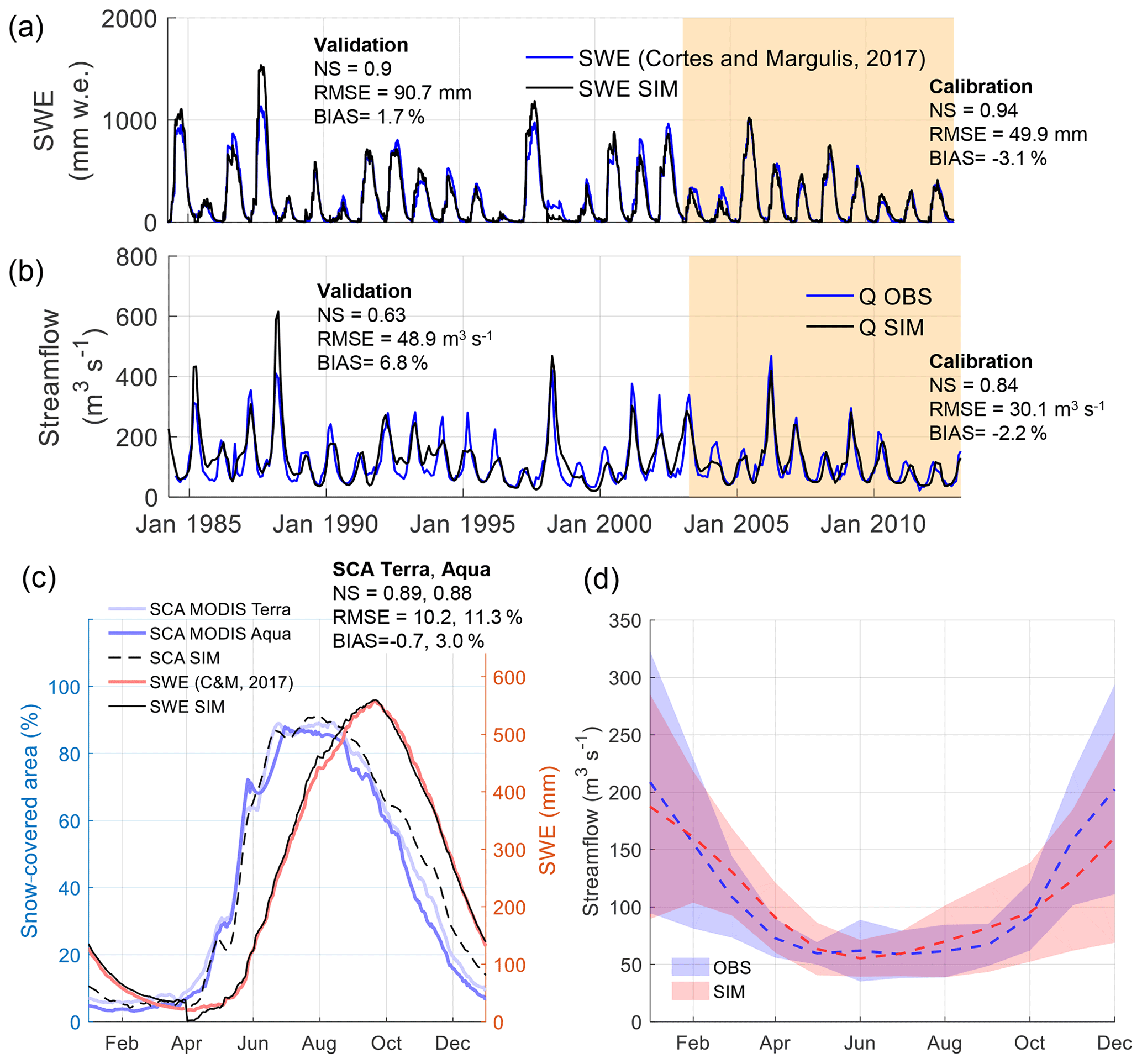
Figure 2Results of the calibration of the TOPKAPI-ETH model for the Maipo River basin. (a) Simulated SWE against results of Cortés and Margulis (2017). (b) Simulated and observed monthly streamflow at the basin outlet. In (a) and (b) the light orange area indicates the calibration period. (c) Average seasonal variability of simulated and observed SCA from the Aqua and Terra missions and SWE from Cortés and Margulis (2017) in the calibration period. (d) Average seasonal variability of simulated and observed streamflow in the calibration period. The colored areas in (d) correspond to the observed and simulated standard deviations from the interannual variability. Model metrics are indicated for the calibration and validation periods and correspond to the following terms: Nash–Sutcliffe coefficient (NS), root-mean-square error (RMSE), and average bias (BIAS).
Figure 2 shows the results of the model calibration for daily time series of SWE (Fig. 2a); monthly time series of streamflow (Fig. 2b); and seasonal variations in SCA (Fig. 2c), SWE (Fig. 2c), and streamflow (Fig. 2d). The final calibrated snow parameters for this setup are shown in Table 1, whereas values for the subsurface flux parameters are shown in the Supplement (Table S1). The quality metrics for snow and streamflow variables show very good results in both the calibration and validation periods. Extreme values are well captured, except for the humid winter of 1988, in which the model underestimates snow accumulation and streamflow.
Table 1Parameters in TOPKAPI-ETH's snow and ice modules for the 1955–2016 time period. The tested ranges of some parameters are given in parentheses.

4.1.3 Model setup for individual glaciers
In addition to the basin-scale model, we set up an instance of TOPKAPI-ETH for each one of the glaciers larger than 1 km2 in the catchment (about 59 glaciers). These instances have a spatial resolution of 100 m, which is more adequate to simulate the processes governing glacier mass balance. The domain of these models runs correspond approximatively to the smallest catchment that contains the 1955 glacier extent of each glacier. The models are run at a daily time step starting in the year 1955 and are then restarted in 2000 using the topographic and geographic information from that year. The models are forced using daily precipitation at the location of the centroid of each glacier, linearly interpolated from basin-averaged precipitation (including the 50 % precipitation correction) (Alvarez-Garretón et al., 2018), and assumed to be uniform over each corresponding domain. Air temperature is extrapolated from the Embalse El Yeso meteorological station using a constant air temperature gradient equal to the environmental lapse rate (−6.5 ∘C km−1). For the study period in which no CR2 precipitation products are available, the Quinta Normal and Embalse El Yeso stations are used.
We choose a set of model parameters typically used in the literature for this region (Ragettli and Pellicciotti, 2012; Ayala et al., 2016; Burger et al., 2019) for all individual glacier models and keep parameter calibration at a minimum level. For each glacier, we vary only the ETI model parameters within ranges suggested in the literature (Finger et al., 2011; Ragettli and Pellicciotti, 2012; Ayala et al., 2017b) to fit the glacier-wide mass balance as derived from the geodetic mass balances. Glacier-wide mass balance is considered fitted when the difference between the simulated and observed balance is smaller than a certain threshold. We find that choosing a threshold equal to half of the uncertainty in the geodetic mass balance allows for reliable simulations while keeping an acceptable computation time. The uncertainty of the geodetic mass balances are 3.2 and 1.2 m w.e. for the periods 1955–2000 and 2000–2003, respectively. In contrast to the model setup for the entire Maipo River basin, in this setup we do not perform any corrections to account for sublimation or other mass removal apart from melt. However, as these models are calibrated on volume loss (thus including both losses by sublimation and melting), it can be assumed that glacier response is well captured, but the portioning of hydrological fluxes (sublimation versus runoff) is unconstrained. A summary of literature-derived and calibrated parameters for the individual models is shown in Table 1. Within each model, melt factors for debris-covered areas are fixed to 25 % of the values for debris-free areas. The 25 % factor is estimated from the comparison between melt rates on debris-free and debris-covered sites on Piramide, Bello and Yeso glaciers in the Estero del Yeso catchment (Ayala et al., 2016; Burger et al., 2019), a sub-catchment of the Maipo River basin.
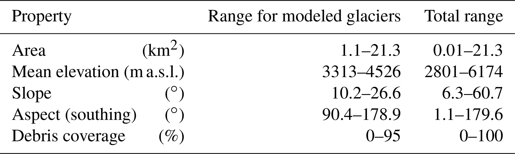
Although we set up a TOPKAPI-ETH model for all glaciers with an area above 1 km2 in 2000 (equivalent to 59 glaciers), we find that staying within the selected ranges for the ETI parameters only allows us to fit the geodetic mass balances in 26 cases. Among the discarded glaciers, about half of them are smaller than 3 km2, and the rest correspond to those lying on the slopes of the Tupugatito Volcano and San José volcanic complex (Volcán Tupungatito, Azufre, and Marmolejo glaciers). We suspect that this is an expression of the fact that some of the processes not included in TOPKAPI-ETH (namely permafrost, sublimation, snow dynamics, or geothermal fluxes) may play a role governing the mass balance of these glaciers. However, it might also be related to local deficiencies in the spatial distribution of air temperature and precipitation. No rock glaciers are included in this subset of glaciers. The location and main properties of the 26 modeled glaciers in comparison with those of the total sample are shown in Fig. 3 and Table 2, respectively. The simulated glaciers are spread over the entire basin, and their mean elevations are in the middle range of the total sample. Glaciers smaller than 1 km2, from which 85 % correspond to rock glaciers or glacierets, are less well represented by the sample of 26 glaciers. The sample of 26 glaciers is mostly oriented towards the south (aspect >90∘) and does not include the steepest glaciers. In Fig. 3, we also highlight the areas with the discarded large glaciers on Tupungatito Volcano and the San José volcanic complex.
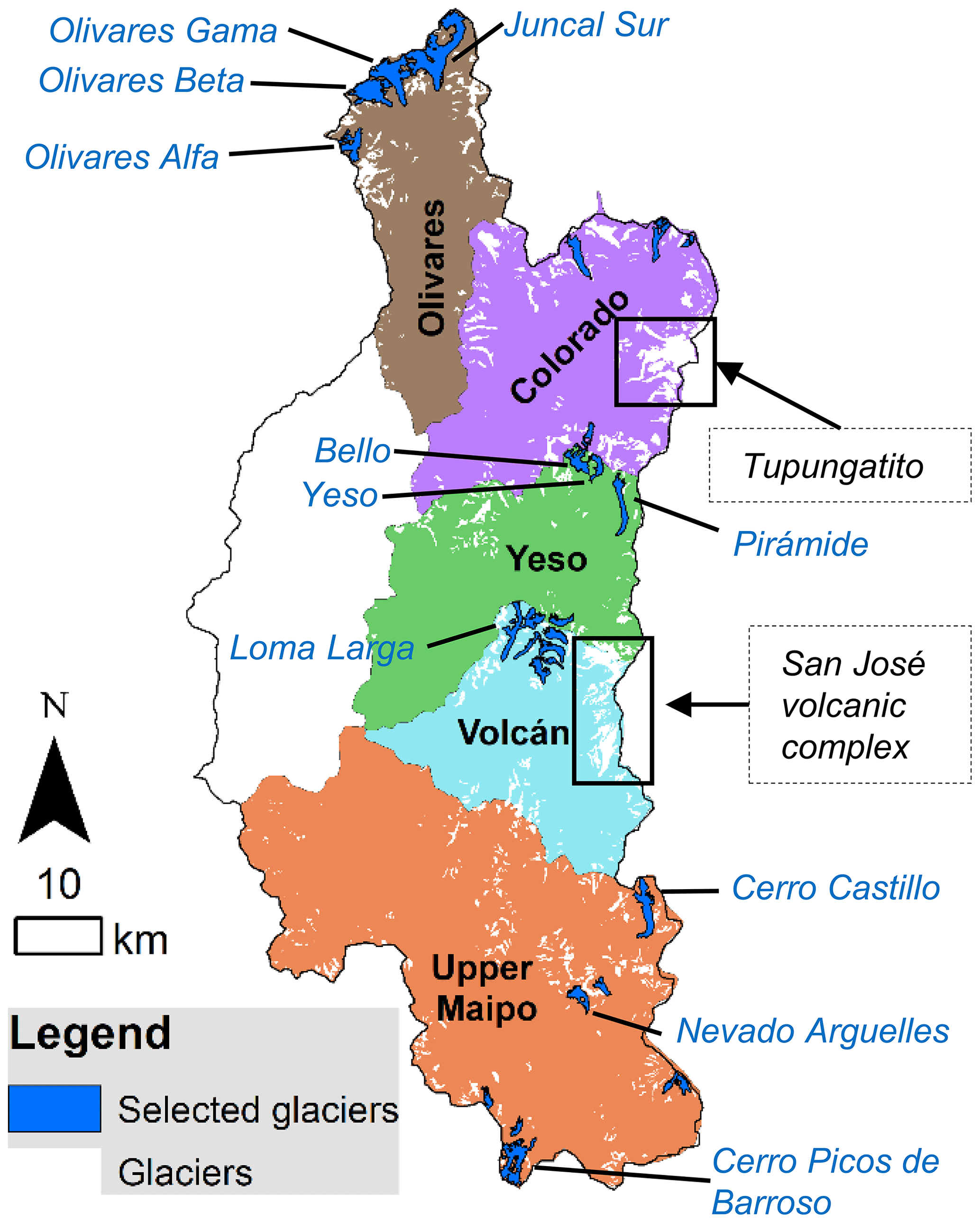
Figure 3Location of the 26 glaciers modeled with TOPKAPI-ETH. We highlight the volcanic areas in which some large glaciers were discarded from the modeled sample. We include the name of the main glaciers in this sample.
Table 2Morphological properties of the 26 glaciers modeled with TOPKAPI-ETH
The results of the calibration of the TOPKAPI-ETH models for the 26 modeled glaciers are shown in Fig. 4a (1955–2000) and Fig. 4b (2000–2013). The calibration results are very good for both periods with area-weighted RMSEs of 1 and 0.2 m w.e. for the 1955–2000 and 2000–2013 periods, respectively. These errors are well within the uncertainty bounds of the geodetic mass balance. Figure 4c shows the resulting cumulative glacier mass balance for all simulated glaciers, their area-weighted average, and the comparison with the glaciological mass balance measured on the Echaurren Norte Glacier since 1975. The fastest declining line of the sample corresponds to the Olivares Alfa Glacier, which has been previously identified as one of the glaciers with the largest retreating rates in the basin (Malmros et al., 2016). Interestingly, several of the glaciers show a positive or near-neutral mass balance over the entire period, which might be an indication that these glaciers have already retreated close to a new equilibrium. However, this is not the general trend in the basin (as shown by the average values in Fig. 4), and it is limited to some specific cases where glaciers have retreated to elevations above the basin-average ELA, or have been covered by thick debris.
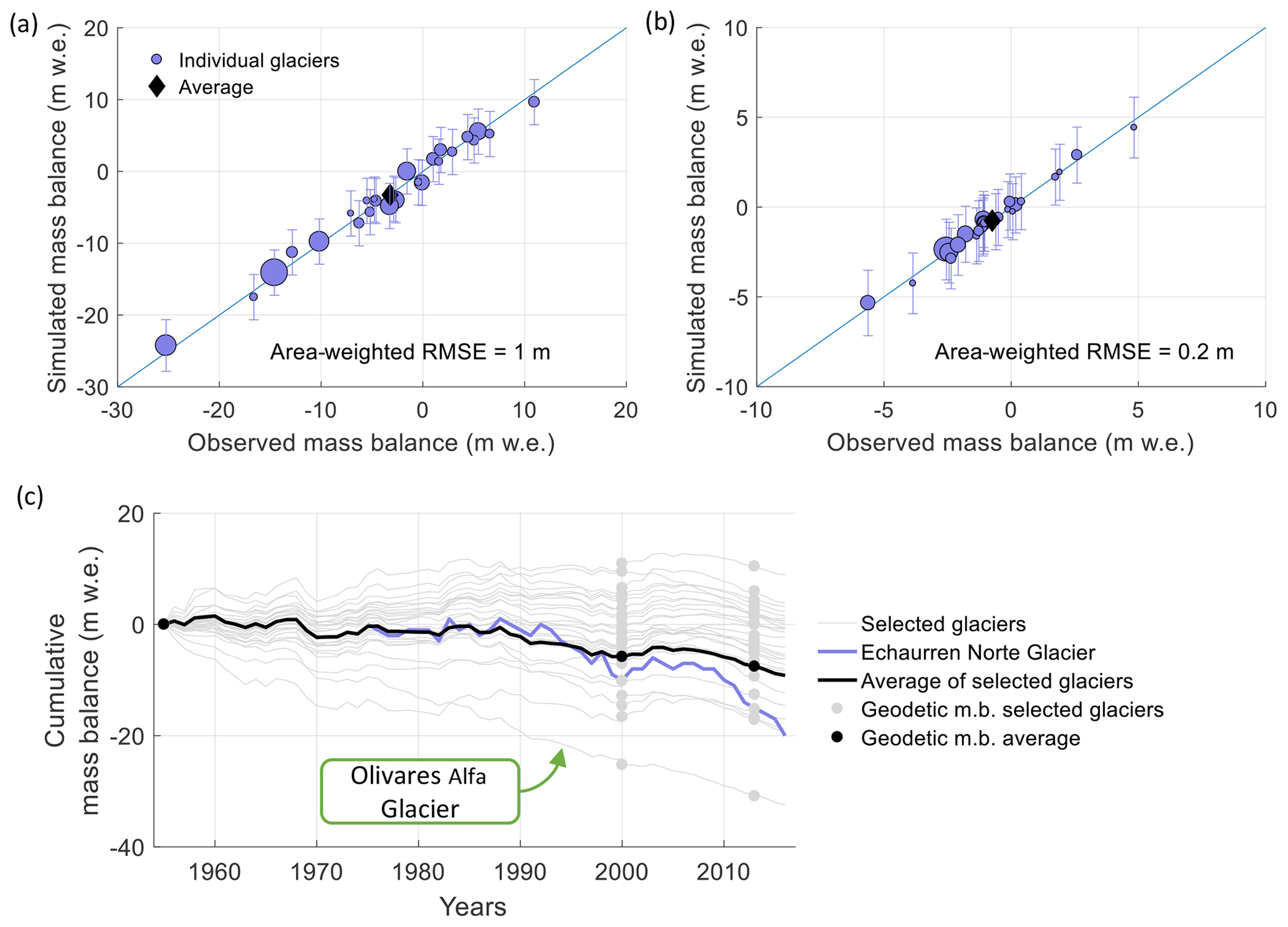
Figure 4Results of the calibration for the 26 modeled glaciers. Glacier-averaged mass balance (blue circles) simulated with TOPKAPI-ETH and observed from geodetic mass balances in the period (a) 1955–2000 and (b) 2000–2013. The area-weighted average of all glaciers is indicated with black diamonds. The blue bars show the uncertainty of the geodetic mass balances. (c) Cumulative 1955–2016 mass balance for each modeled glacier (grey lines), the area-weighted average of all glaciers (black line), and the mass balance measured on Echaurren Norte Glacier (blue line) are also shown. The geodetic mass balances for each modeled glacier is indicated with a circle. The curve corresponding to the fastest retreating glacier of the sample, Olivares Alfa Glacier, is labeled.
4.2 Extrapolation
We extrapolate the mass balance of the 26 modeled glaciers to the entire basin based on the methodology described by Huss (2012). In that work, a set of in situ glacier mass balance measurements for Switzerland were used to calculate the mass balance of all glaciers in the European Alps. Here, we calculate the annual surface mass balance B (m w.e.) of glacier g in year y with the following equation:
where is the average annual mass balance in the study period p and ΔB(s,y) is the glacier annual mass balance anomaly in the sub-catchment s, where glacier g is located. While is extracted from the geodetic mass balance, ΔB(s,y) is derived from the TOPKAPI-ETH simulations. Equation (4) is applied to the periods 1955–2000 and 2000–2013 by calculating from the geodetic mass balance. The term ΔB(s,y) is calculated as the anomaly of annual mass balance of simulated glaciers located in the sub-catchment s for each study period, i.e.,:
where is the subset of modeled glaciers (∗) in sub-catchment s.
The time series of annual mass balance B(g,y) are then used to estimate the volume changes of each glacier throughout the study periods. Glacier areas (S) are updated due to negative changes in glacier volume (V) (we do not prescribe increases in glacier area due to positive annual mass balance) by means of the volume–area scaling formula:
where γ and c are the scaling parameters. In line with recommendations of the volume–area scaling theory (Bahr et al., 2015), the parameter γ is kept constant in all periods at a value of 1.357, and we let c vary in order to fit the total glacier volume in the basin in years 1955 and 2000 (calculated in Sect. 3.2). Parameter c is calculated as 28.1 for 2000 (this value is also used afterwards), but a value of 21.1 is the one that fits best to our estimates of ice thickness in 1955. In between these 2 years we use a linear interpolation of c. In the calculation of area and volume evolution, we account for the uncertainties in the annual mass balance, inventoried glacier areas in 1955 and 2000, and the parameter c, by disturbing each variable with a random variation. These random variations are 1000 realizations of three normal probability distributions of mean 0 and standard deviations equivalent to the typical errors of each variable. From the uncertainties in the geodetic mass balance, we estimate a typical error in the annual mass balance of 0.08 m w.e. yr−1 for the period 1955–2000 and 0.13 m w.e. yr−1 for 2000–2016. Based on Paul et al. (2013), we assign a 5 % error to the area of each glacier in the year 2000 inventory, and we double this value for the 1955 inventory. The error for the parameter c is calculated in order to match the uncertainty in our ice thickness estimates, and results in a value of 4.1. The uncertainty in parameter c should indirectly account for the different boundary conditions (such as basal sliding or surface geometry) that are found at each glacier (Bahr et al., 2015).
Glacier runoff, including all its components (i.e., ice melt, snow melt and rain), is extrapolated directly from the TOPKAPI-ETH results for the 26 modeled glaciers to the rest of the glacierized areas. At a particular year, the uncertainty in glacier runoff is estimated as a fraction of the same variable. That fraction is the same as that between glacier volume and its uncertainty in that year. As in Huss and Hock (2018), we compute glacier runoff as the water originating from the initially glacierized area (1955 in our case), i.e., independent of the glacier area in a particular year. This allows for the evaluation of changes in total headwater runoff due to glacier retreat. However, in our study we also evaluate specific variations in the ice melt component. Throughout this paper, glacier runoff and its components are presented as normalized by the area of the entire Maipo River basin.
4.3 Committed ice loss estimates
We estimate the committed glacier ice loss caused by the temperature increase in the last decades by conducting a set of 10 additional TOPKAPI-ETH simulations, and by extrapolating them using the same procedure as described in the previous section. The additional simulations are run under different synthetic climate scenarios in which the climate of the last 2 decades is stochastically repeated for a 100-year period. The meteorological inputs are built by repeating 1-year-long blocks of the input variables (precipitation, temperature, and cloud transmissivity) corresponding to a randomly selected year between 1993 and 2016 (23 years). We select this period because air temperature was relatively stable in the basin and precipitation showed the characteristic interannual variability of this region.
While the anomaly term ΔB(s,y) is calculated in the same way as for the period 1955–2016 (i.e., from the TOPKAPI-ETH simulations), as no geodetic mass balances are available for the synthetic scenarios, we calculate using two different approximations depending on glacier size. For glaciers that are larger than the size of the smallest modeled glacier (1.1 km2), we use a multiple linear regression of the mass balance of the modeled glaciers in each scenario with their topographic parameters in year 2000:
where ai are calibrated coefficients and xi are topographic parameters. In average for the 10 synthetic scenarios, the best results are given by glacier area, median glacier elevation, percentage of debris cover, mean sky view factor, and mean aspect. Together, these five variables explain 52 % of the total variance, which is in the range of the original application of this methodology (which obtained 35 % using three variables and 51 % using six; Huss, 2012). Results of this procedure are summarized in Table 3. For glaciers smaller than 1.1 km2, we use the average mass balance of modeled glaciers in the corresponding sub-catchment. As in the 1955–2016 period, rock glaciers are assumed to have a balanced mass budget. Once the time series of mass balance for the 10 synthetic scenarios are calculated, we compute area and volume evolution of each glacier and their associated uncertainties, using the same methodology as for the 1955–2016 period.
Table 3Results of the multiple regression analysis for the committed ice loss scenario simulations.
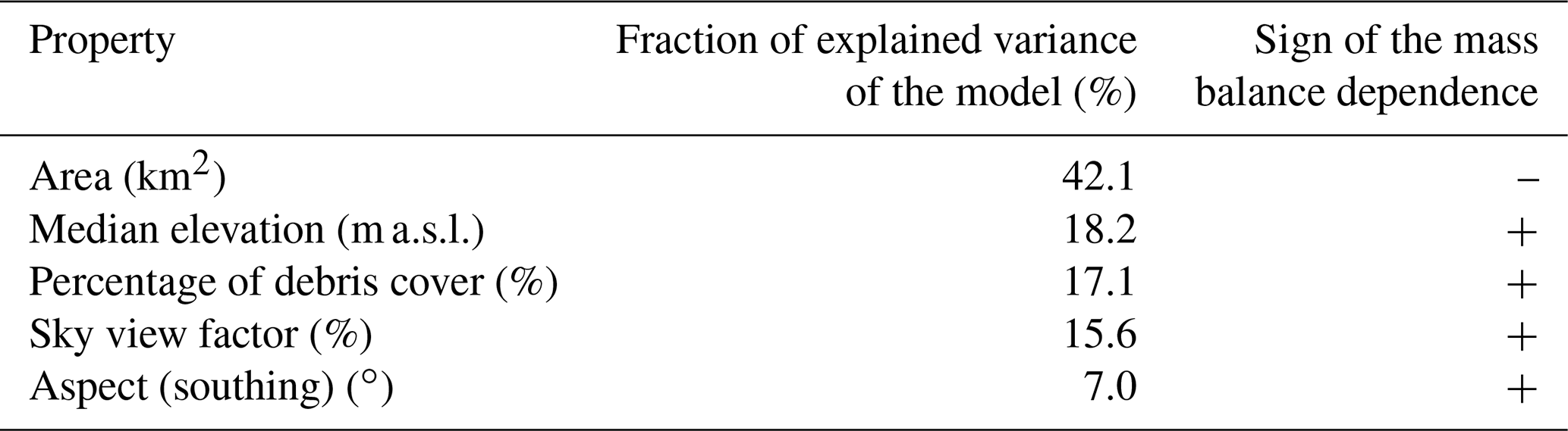
Figure 5 and Table S2 (in the Supplement) present a summary of the simulations in this study. In the period 1955–2016, we conduct the TOPKAPI-ETH simulations for the Maipo River basin (SIM-1A), the 26 modeled glaciers (SIM-1B), and the extrapolation for all glaciers (SIM-1C). Using the synthetic meteorological time series derived to calculate the committed ice loss, we conduct 10 additional TOPKAPI-ETH simulations for the Maipo River basin (SIM-2A) and the modeled glaciers (SIM-2B), which are then also used for extrapolation (SIM-2C).
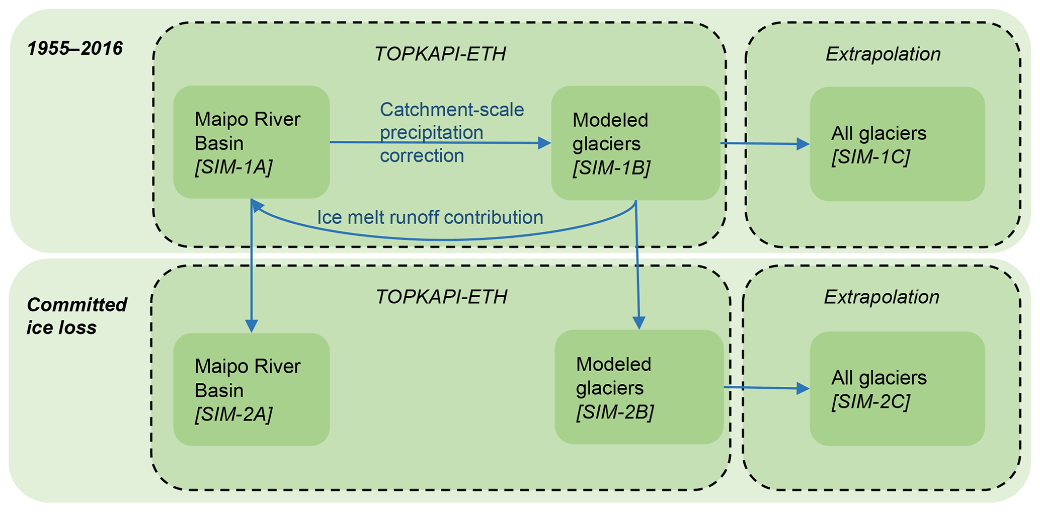
Figure 5Organization of the simulations. The two main boxes indicate the time period of the simulations (1955–2016 and committed ice loss scenario), the boxes with a dashed outline indicate the method used (TOPKAPI-ETH or extrapolation), and the smallest boxes indicate the spatial domain (Maipo River basin, modeled glaciers, and all glaciers). The arrows indicate outputs that are used in other methods or domains. The codes in brackets (e.g., SIM-1A) correspond to the simulation codes defined in Table S1.
5.1 Glacier changes and runoff contribution in the period 1955–2016
In Fig. 6, we present the temporal variability of precipitation (Fig. 6a), air temperature (Fig. 6a), the equilibrium line altitude (ELA) (Fig. 6b), and cumulative mass balance (Fig. 6c and d) in the Maipo River basin since 1955. While the large interannual variability of the basin's mean precipitation (Fig. 6a, blue bars) directly relates to the El Niño–Southern Oscillation (ENSO) phenomenon, a 3-year moving average of this variable exposes a sequence of dry (e.g., 1967–1969, 2010–2016) and wet periods (e.g., 1978–1987 and 2000–2008). This sequence has been related to other climatic indices, such as the Pacific Decadal Oscillation (PDO) or the Interdecadal Pacific Oscillation (IPO) (Boisier et al., 2016; González-Reyes et al., 2017). From 2010 on, precipitation has decreased due to a severe drought across Chile (Garreaud et al., 2017). Air temperature over the basin shows a sustained increase in the long term but with relatively stable values since the mid-1990s. Since the 1960s, air temperature has increased in about 2 ∘C. Figure 6b shows the annual and decadal variability of the ELA of the 26 modeled glaciers. The ELA is calculated as the average elevation of all grid cells with an annual mass balance of ±10 cm, and the estimated range (in light red) corresponds to the standard deviation. Since the 1960s, the elevation of the ELA has increased by 239 m (or 39 m per decade). These estimates of the ELA change are larger than those calculated by Carrasco et al. (2005), who estimated an increase in the elevation of the 0 ∘C isotherm of about 160 m for central Chile in the period 1975–2001.
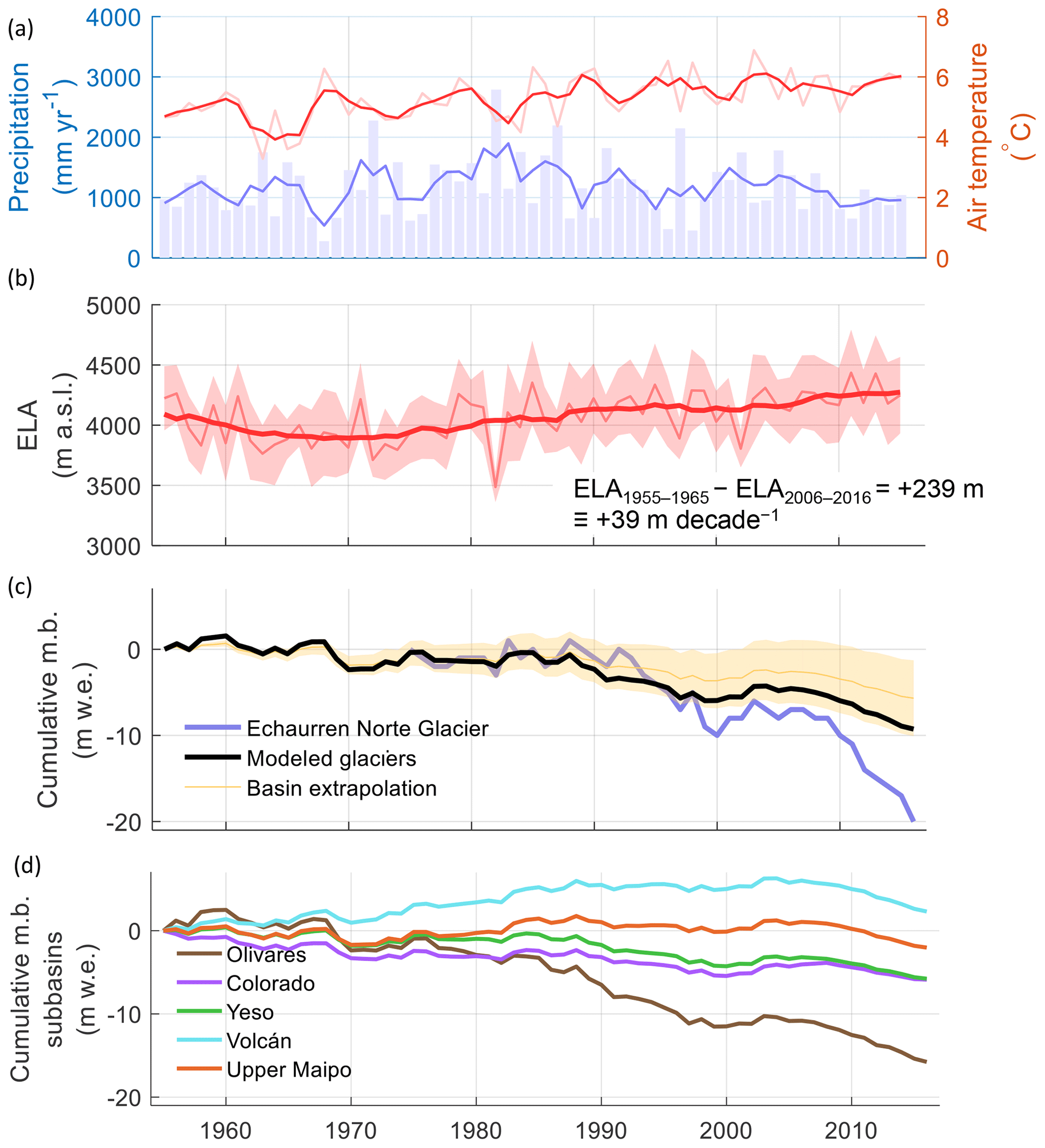
Figure 6Variability of meteorological and glaciological variables in the Maipo River basin over the period 1955–2016: (a) air temperature and precipitation with a 3-year moving mean; (b) equilibrium line altitude (ELA); (c) cumulative glacier mass balance for the modeled glaciers (simulated with TOPKAPI-ETH), the entire basin (extrapolation) and its associated uncertainty, and the measurements on Echaurren Norte Glacier; and (d) cumulative glacier mass balance for each sub-catchment. In (b) the difference between the ELA in the last 10 years (2006–2016) and the first 10 years (1955–1965) of the study periods is indicated, as is the equivalent ELA increase rate. The shadowed area in (b) shows the standard deviation of the elevation of grid cells with a mass balance between −0.1 and 0.1 m w.e.
Figure 6c and d integrate the results of TOPKAPI-ETH and the extrapolation procedure. Figure 6c presents the cumulative surface mass balance of glaciers in the Maipo River basin since 1955, including the 26 glaciers modeled with TOPKAPI-ETH, and the remaining glaciers in the basin for which extrapolation was used. The cumulative mass balance shows a decreasing trend interrupted by short periods of positive or near-neutral mass balance, with a more negative final value for the 26 modeled glaciers than for all glaciers in the basin. The more negative value for modeled glaciers might be caused by their larger area in comparison to the rest of the glaciers, as large glaciers have shrunk more extensively (Malmros et al., 2016). For comparison with the long-term glacier mass balance reference in the region, we include the direct measurements on Echaurren Norte Glacier, which presents a more negative trend, most likely due to its low elevation (3650 to 3900 m a.s.l.). In Fig. 6d, we present the surface mass balance of glaciers in each sub-catchment, where relatively large differences can be seen. In general, glaciers in southern catchments show more positive mass balance than those in northern catchments. This can be explained by larger precipitation amounts and a higher proportion of both debris-covered and rock glaciers. Most notably, glaciers in Olivares show the most negative mass balance throughout the study period, whereas those in Volcán present a positive mass balance until the mid-2000s. However, after the start of the current drought in 2010, negative glacier mass balances dominate across the entire Maipo River basin. The information included in Fig. 6d is summarized in Table 4, which shows the simulated glacier mass balance in each sub-catchment for the 1955–2016 period. For comparison, we include the mean elevation, mean latitude, and the 1955 glacierized area of each sub-catchment.
Table 4Simulated glacier mass balance and runoff in the sub-catchments compared with their main characteristics
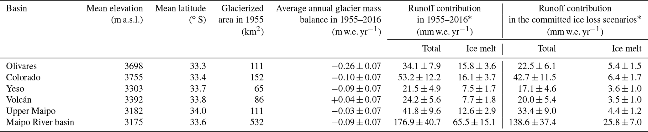
* From the areas defined by the 1955 glacier outlines but normalized by the Maipo River basin area
In Fig. 7 we show the variations in glacier runoff and its components (ice melt, snow melt and rain) in the initially glacierized areas over the period 1955–2016. While the annual and summer interannual variability is presented in Fig. 7a and b, Fig. 7c presents the average seasonal curve and the percentage of each contribution. The summer period is chosen as January to March. Glacier runoff was 177±25 mm yr−1 over the entire period and shows a sequence of three decreasing maxima (1968–1969, mid-1980s, and the end of 2000s). Glacier runoff peaked at 245±62 mm yr−1 during the severe drought of 1968–1969 (the driest hydrological year on record), and it averages 158±27 mm yr−1 during the current drought (2010–2016). Figure 7a shows that the interannual variability of ice melt is very large (with a coefficient of variation of 0.57) and that its share in total glacier runoff can vary from less than 10 % (as in 1982–1983, 1997–1998, and 2002–2003) to more than 90 % (as in 1968–1969). Except for 1968–1969, snow melt in these areas is consistently the largest runoff contributor at the annual scale, but the contribution during summer is very variable. In Fig. 7c, we show the summary of runoff contributions at the annual scale. Runoff contribution is dominated by snowmelt (60 %), with ice melt representing 37 % of the annual total. Rain represents about 3 %, but these amounts have increased since 1955 (Fig. 7a and b).
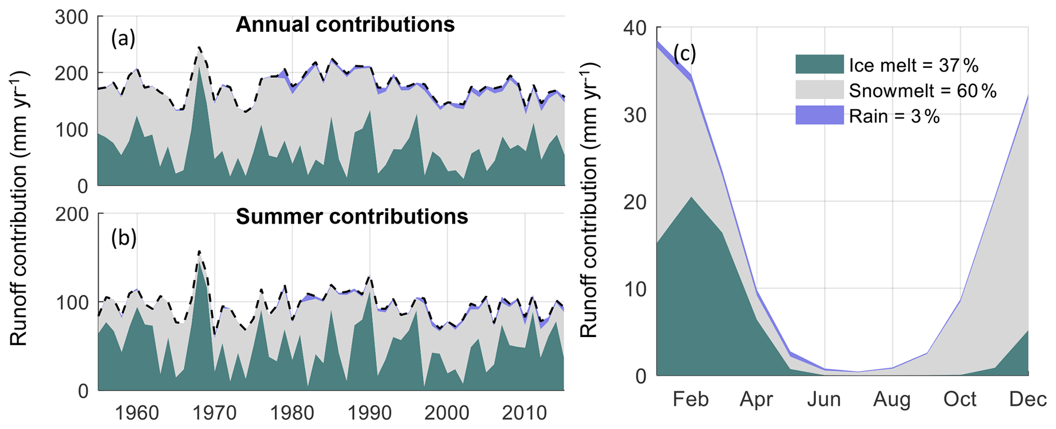
Figure 7Runoff contribution from ice melt, snow melt, and rain from the headwater regions defined by the 1955 glacierized areas. The units are normalized by the Maipo River basin area. (a) Total annual contribution, (b) summer contribution, and (c) seasonal average contribution are given. The percentages of each contribution over the period 1955–2016 are indicated in the legend.
In Fig. 8, we quantify the role that glacier runoff has played in the entire Maipo River basin over the study period. At the annual scale, glaciers provide 16±7 % of the total runoff, but this contribution can increase up to 59±23 % in summer. In 1968–1969, the runoff contribution from the 1955 glacier areas provided 49 % of the annual runoff and almost 100 % during summer. During the current drought, glacier runoff has represented 17 % of the annual runoff and 55 % of summer runoff. The value of 17 % during the current drought is close to the average value over the entire study period.
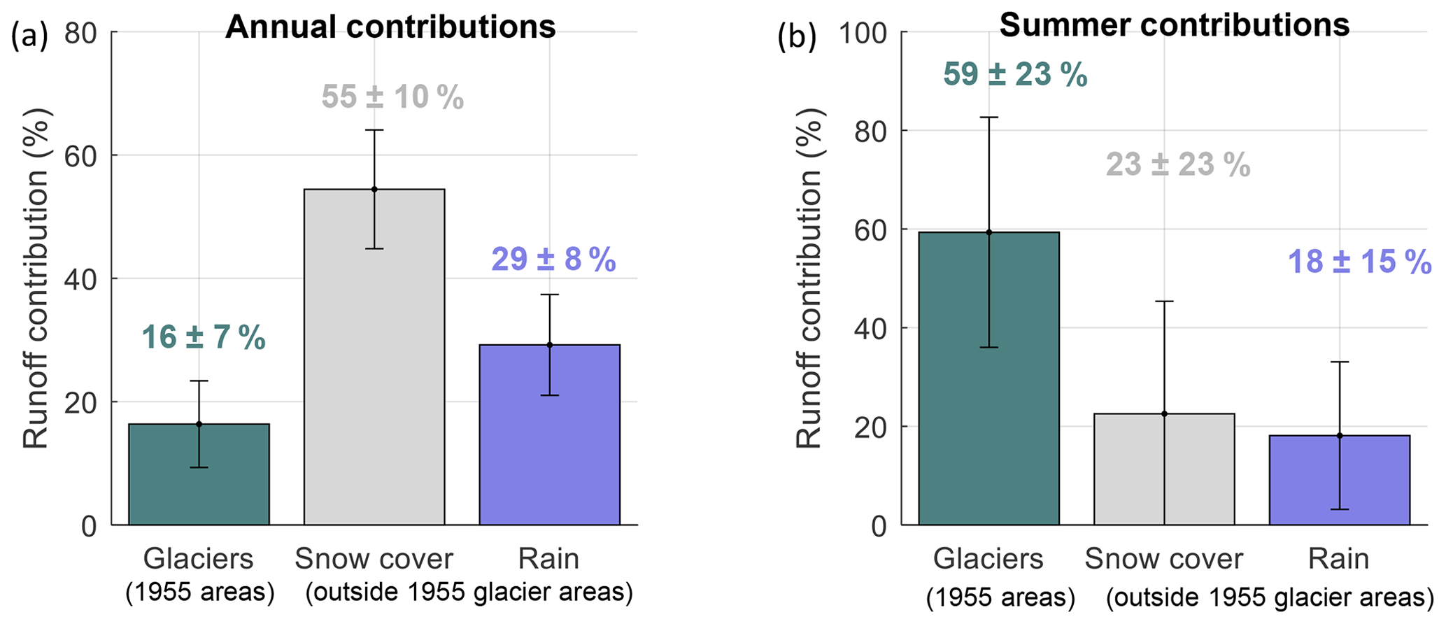
Figure 8Partition of runoff contribution in the Maipo River basin in the period 1955–2016. The contributions are computed for the headwater regions defined by the 1955 glacierized areas (the sum of ice melt, snow melt, and rain) and snow melt and rain outside those areas. The plus and minus symbols refer to the interannual variability. (a) Annual and (b) summer contributions are given.
5.2 Glacier changes and runoff contribution for the committed ice loss scenarios
Figure 9 presents the evolution of glacier volume (a), area (b), and runoff (c) in the Maipo River basin, in the past period (1955–2016) and the committed ice loss scenarios. To assess the changes of glacier area and volume we use the values estimated for the year 2000 as reference, whereas for glacier runoff we use the average in the period 1955–2016. As mentioned above, the committed ice scenarios do not represent a realistic projection for the future, and we use the years of 2000 to 2100 on the x axis for visual purposes only. Glacier area and volume varied by % (from 532±53 to 347±27 km2) and % (from 18.6±4.5 to 14.9±2.9 km3) in the period 1955–2016, respectively, and if glaciers were in equilibrium with the current climate, the glacier area and volume would reduce to 79±18 % and 81±38 % of the 2000 values, respectively. The uncertainty in glacier area and volume derived from our calculations (blue bands) reduces from 2000 on, due to the higher accuracy that we assign to the year 2000 inventory and DEM. In the committed ice loss scenarios, uncertainty starts at similar levels as that of 2000, but as the scenarios differentiate from each other, the uncertainty increases towards the end of the simulation period. Figure 9c presents glacier runoff from the initially glacierized areas normalized by the area of the Maipo River basin. Glacier runoff in the committed ice loss scenario decreases quickly until a relatively steady value is reached at 78±30 % of the average glacier runoff in the 1955–2016 period. This value is equivalent to 61±21 % of that in 1968–1969. Uncertainty bounds in Fig. 9c are proportional to those of the glacier volume.
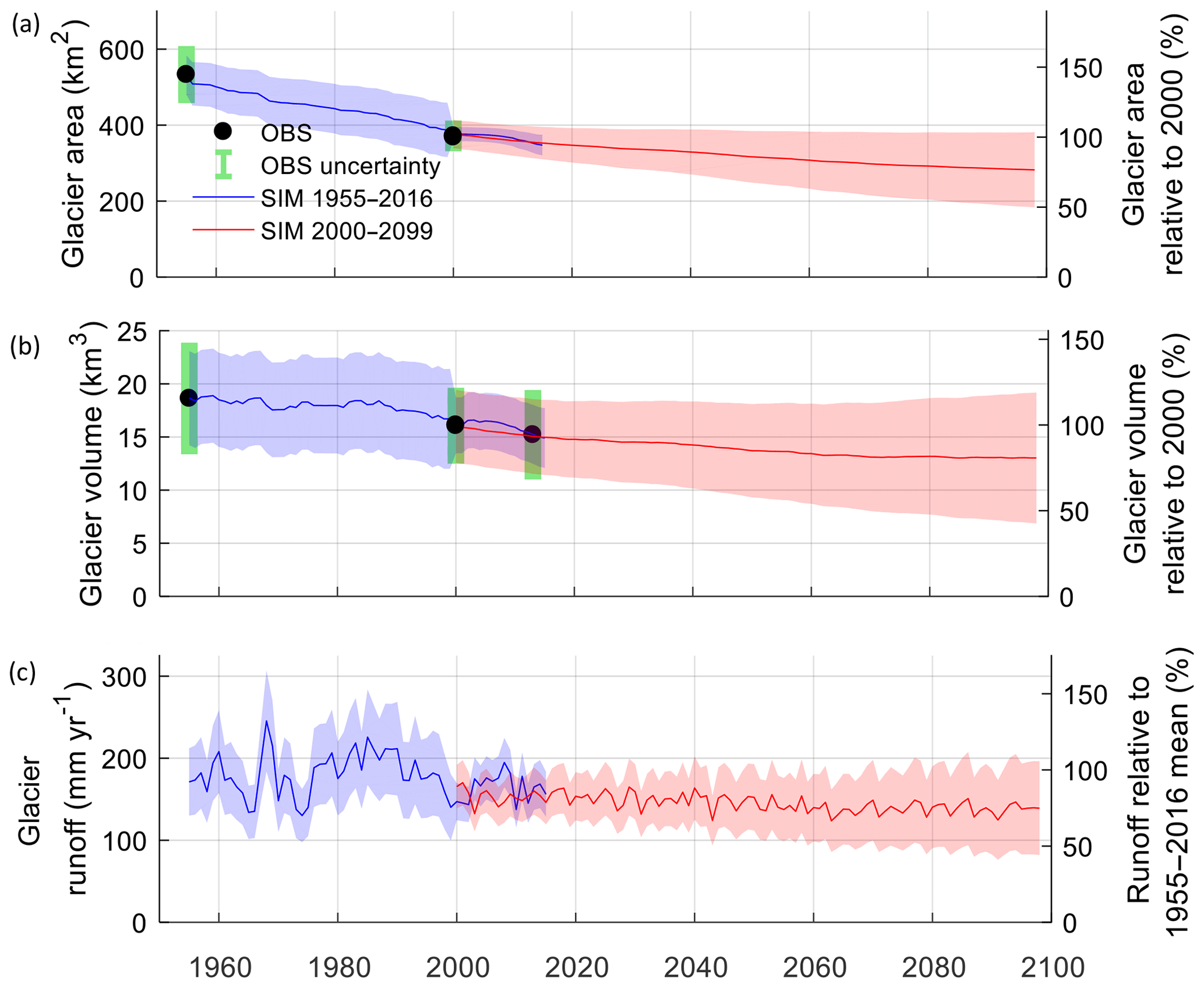
Figure 9Variations in (a) ice volume, (b) glacierized areas, and (c) glacier runoff in the Maipo River basin for the past period (1955–2016) and the committed ice loss scenarios assuming a constant climate. In (a) and (b) we use results from the glacier inventories and the combination of ice thickness estimates and geodetic mass balances, respectively, as observations of glacier area and volume. Glacier runoff in (c) is computed for the Maipo River basin (i.e., runoff units are normalized by the basin area). While the uncertainty bars of the observations are shown in green, those of the simulations are shown in blue for the 1955–2016 period and in red for the committed ice loss scenarios. For visual purposes, we present the committed ice loss scenarios using the period 2000–2100 in the x axis.
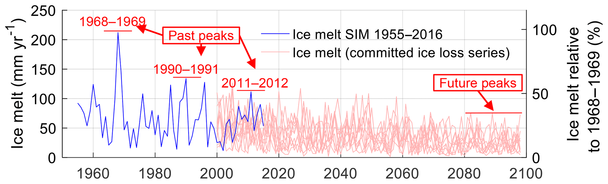
Figure 10Variations in ice melt in the Maipo River basin for the past period (1955–2016, in blue) and each one of the 10 committed ice loss scenarios (light red). The peaks of ice melt over the past period and those at the final decade of the committed ice loss scenarios are highlighted in red. On the right axis, we set the ice melt estimated for the severe drought of 1968–1969 as 100 %. Ice melt is computed for the Maipo River basin (i.e., runoff units are normalized by the basin area). For visual purposes, we present the committed ice loss scenarios using the period 2000–2100 in the x axis.
As the large precipitation interannual and inter-decadal variability could mask the runoff trends associated only with the reduction of glacier volume, in Fig. 10 we present the variability of ice melt in the period 1955–2016 and the committed ice loss scenarios. For this figure, we use the maximum value of ice melt in the period 1955–2016 as reference, which corresponds to the hydrological year 1968–1969. Although ice melt also shows a very large interannual variability, it is clear that the maximum values have decreased over the last decades (see maximum values in 1968–1969, 1990–1991, and 2011–2012). We estimate that if glaciers reached equilibrium with the current climate, the peaks would be considerably lower than those in the 1955–2016 period. In this equilibrium situation, the peaks are close to 40 % of the largest ice melt runoff contribution in the past (1968–1969). The information presented in Figs. 9c and 10 is also summarized in Table 4. In that table, we present the average glacier runoff contribution per sub-catchment for the 1955–2016 period and the last 20 years of the committed ice loss scenarios.
6.1 Glacier changes
Our results indicate that the total glacier volume in the Maipo River basin decreased by about one-fifth in the period 1955–2016. The cumulative glacier mass balance in the Maipo River basin shows variations that are similar to those registered on Echaurren Norte Glacier. These variations consist of a general decreasing trend, concurrent with an increase in the ELA (Carrasco et al., 2005, 2008), which has been interrupted by periods of slightly positive or neutral mass balance. Since the mid-1980s, there has been a strong mass loss, interrupted only by a positive period in the beginning of the 2000s. In fact, from 2000 on, we observe a 10-year period with positive or nearly neutral mass balance. This was also described by glaciological observations (Masiokas et al., 2016) and geodetic mass balances (Braun et al., 2019; Dussaillant et al., 2019). Following this period, strongly negative mass balances have been observed (Masiokas et al., 2016; Burger et al., 2019), concurrent with a severe drought in central Chile, unprecedented in extension and duration (Garreaud et al., 2017). For the period before 1975, when the mass balance measurements on Echaurren Norte Glacier started, we compare our results to the reconstruction obtained by Masiokas et al. (2016). The latter estimated a strongly negative mass balance in the period 1955–1975, while we obtain a nearly neutral mass balance between 1955 and 1968 and a more negative balance from 1968 to 1975. These differences might either correspond to differences between the basin-averaged mass balance and that on Echaurren Norte Glacier or be a consequence of the different methodologies between our study and that of Masiokas et al. (2016). While Masiokas et al. (2016) relied on the correlation between hydrometeorological records and the measured surface mass balance on Echaurren Norte, our model is calibrated to the geodetic mass balances.
The different trends of glacier mass balance in the sub-catchments of the Maipo River basin are an expression of the diverse climatic and morphological characteristics that dominate across the basin. For example, the positive and near-neutral glacier mass balances in Volcán and Upper Maipo might be related to higher precipitation towards the south or that several glaciers have retreated close to a new equilibrium state. Within the Olivares sub-catchment, the geodetic mass balance is in line with the large areal changes found by Malmros et al. (2016). This might be explained by a strong imbalance of the large glaciers in that catchment and/or by the impacts of nearby mining activities (Los Bronces and Andina mines), especially dust deposition on Olivares Alfa Glacier and its neighbor glaciers. However, more specific studies addressing albedo changes are necessary to obtain more conclusive results.
Our estimates of committed ice loss show that glaciers will continue to shrink if the climate remains stable, with an estimated committed ice loss of 20 % relative to the volume in the year 2000 (30 % relative to 1955). We stress that these estimates are an indication of the glacier changes that past climate will produce in any case. Future projections under emission scenarios will certainly show more dramatic reductions of glacier area and volume. In the context of future projections, we highlight that most projections for glacier changes in the Central Andes (Marzeion et al., 2012; Radić et al., 2014; Huss and Hock, 2015) are included in the macro-region of the “southern Andes”, which also contains the Patagonian Ice Fields. Future projections of glacier changes in the region are thus strongly influenced by these large ice masses with their peculiar climate and physical processes (e.g., calving) that are not representative of the small mountain glaciers along the semiarid Andes (Mernild et al., 2015).
6.2 Glacier runoff
Despite the reduction of glacier volume in the period 1955–2016, our estimates of glacier runoff do not show (Figs. 8 and 9c) the typical increasing or decreasing phases of peak water observed or projected for other catchments across the world (Baraer et al., 2012; Farinotti et al., 2012). This result is similar to that obtained by Casassa et al. (2009), who did not find significant trends in an analysis of Maipo streamflow records. Peaks in glacier runoff have reduced their magnitude over the last decades, due to a combination of a decrease in precipitation (Boisier et al., 2016) and the reduction of ice volume, but it is difficult to identify if there was an increasing phase of glacier runoff in the period 1955–2016.
We suggest that the strong interannual and inter-decadal climatic variability observed in the semiarid Andes (Montecinos and Aceituno, 2003; Masiokas et al., 2006; Falvey and Garreaud, 2007) is also transferred to the glacier runoff time series, modifying or masking the typical trends associated with glacier retreat. Once an extended time period is considered (in this case a committed ice loss scenario, Fig. 9c), peak water emerges more clearly. Huss and Hock (2018) estimated that glacier runoff in the Rapel River basin (south of the Maipo River basin) experiences peak water in the current decade (2010–2020), but their analyses also show a strong interannual glacier runoff variability from 1980 to 2010. This makes peak water evident only when compared to the future projections under different emission scenarios, in which the glacier runoff is considerably lower than present levels.
6.3 Uncertainties in the modeling of glacier changes in data-scarce regions
We identify four main sources of errors and uncertainties in our study: (i) the glaciological datasets, i.e., the geodetic mass balance, glacier outlines, ice thickness, and debris cover areas; (ii) the spatial distribution of meteorological inputs; (iii) modeling limitations in TOPKAPI-ETH; and (iv) limitations of the extrapolation methodology.
In general, the uncertainties of the elevation changes and glacier properties are well quantified and explicitly stated in the confidence bounds of the geodetic mass balance (Fig. 9). However, a few properties were not explicitly quantified, such as the ice content in rock glaciers, which is in fact a key problem in the semiarid Andes (Schaffer et al., 2019). Due to this, there might be an overestimation in the ice content due to the presence of rock glaciers. In the future, more geophysical measurements to acquire information on ice content in rock glaciers of the semiarid Andes (e.g., Croce and Milana, 2002) could improve the estimates of runoff generation from these landforms.
The accuracy in the spatial distribution of meteorological inputs is particularly difficult to evaluate, and it likely corresponds to a major source of uncertainty (especially precipitation). This is because of the relatively sparse network of meteorological stations installed in the basin, the difficulties of atmospheric models to represent precipitation processes over the Andes (Bozkurt et al., 2019), and the underestimation of satellite-based precipitation products over high-elevation areas (Alvarez-Garretón et al., 2018). However, the indirect evaluation of precipitation amounts through snow cover products and the basin's water balance increase the confidence in the results of this study. An additional simplification in the meteorological distribution is the extrapolation of air temperature from one single station. Nevertheless, we are confident that air temperature variability is well constrained over the catchment because it usually correlates well over long distances, daily lapse rates are derived from the basin-wide CR2 temperature dataset, and the timing of snow disappearance is well simulated by TOPKAPI-ETH.
Although our study has benefited from a series of new meteorological and glaciological datasets presented for the southern Andes in recent years (Cortés and Margulis, 2017; Alvarez-Garretón et al., 2018; Farías-Barahona et al., 2020), the lack of field data in the Maipo River basin is something that needs to be taken into account in glacio-hydrological modeling studies in the region, particularly at remote high-elevation sites. In this study, we alleviate the difficulties posed by the lack of basin-wide field data, and its impact on the TOPKAPI-ETH results, by deriving most of the model parameters from data collected in previous field campaigns in this region starting in 2008 (Pellicciotti et al., 2008; Ragettli and Pellicciotti, 2012; Ayala et al., 2016). These previous studies have also shown that many of the parameters required by the model are fairly stable, in the sense that they can be extrapolated from one glacierized area to another with a reasonable degree of confidence (Ragettli et al., 2014; Ayala et al., 2017b; Burger et al., 2019). In addition, the representation of processes driving the mass balance at some specific sites requires more fundamental work, and additional parameterizations or more physically based representations are required. Such sites correspond mainly to sublimation-dominated sites above 5500 m a.s.l., where we had to correct our simulations of snow depth and the temperature index modeling is inaccurate (Ayala et al., 2017a, b), debris-covered areas with complex distributions of debris thickness (Burger et al., 2019), or steep glacierized slopes such as the volcanoes in the Maipo River basin.
As the average rates of annual mass balance in the 1955–2016 period are calculated from the geodetic mass balance, the long-term glacier changes derived from the extrapolation methodology should be well simulated, but the year-to-year variations in mass balance depend on the representativity of the modeled glaciers. As discussed by Huss (2012), low representativity of the reference glaciers could lead to large errors in the mass balance of individual glaciers and years, but these errors should be lower at the mountain range scale and over long time periods. In the committed ice loss scenarios, the uncertainty of glacier changes is higher because it also relies on the multiple linear regression analysis. In any case, we explicitly accounted for the uncertainties in the extrapolated mass balance (at least partly) by means of the random perturbation described in Sect. 4.2.
We have reconstructed the changes that glaciers in the Maipo River basin experienced over the last 6 decades, with a focus on glacier runoff and the impacts of its long-term variations on the basin's hydrology. These results add a missing piece to the current hydro-climatological knowledge of the semiarid Andes and can be useful for water managers and stakeholders to develop adaptation or mitigation strategies. Although some uncertainties still remain, our results successfully take into account a number of independent datasets, including snow cover area variations, snow water equivalent reconstructions, streamflow records, glacier inventories, and geodetic mass balances.
Our main conclusions are as follows.
- a.
Over the period 1955–2016, the total glacier volume in the Maipo River basin has decreased by 20±14 % (from 18.6±4.5 to 14.9±2.9 km3). In agreement with other studies, our results show that the cumulative glacier mass balance over the study period had a general decreasing trend, interrupted by short periods of positive or near-neutral mass balance. This might be an indication that some glaciers temporarily retreated to a new equilibrium state. Strongly negative mass balances have dominated since the start of the current drought in 2010. Despite the general trend, there are important differences between the glacier mass balances of the sub-catchments, with the southern sub-catchments (Volcán and Upper Maipo) showing positive or near-neutral mass balances until 2000 and the Olivares sub-catchment showing a strongly negative mass balance over the entire period.
- b.
The average glacier contribution to runoff in the Maipo River basin (i.e., the runoff contribution from liquid precipitation, snowmelt, and ice melt from the areas that were glacierized in 1955) was 177±25 mm yr−1 in the period 1955–2016. Instead of a clear peak water, we identify a decreasing sequence of runoff maxima that can be linked to both a decrease in precipitation since the 1980s and a reduction of ice melt. The exact occurrence of peak water will also depend on future changes (e.g., more precipitation or more ice melt), which are not addressed in our article. Glacier runoff has decreased since the severe drought of 1968–1969, when glacier runoff peaked at 245±62 mm yr−1 (49 % of the basin's total runoff). During the current drought, which started in 2010, the contribution has been 158±27 mm yr−1 (17 % of the total runoff).
- c.
If climate was to stabilize at the level of the past 2 decades, we estimate a committed glacier ice mass loss of 19±38 %. This would cause glacier runoff to reduce by 22±30 % when compared to the 1955–2016 average or by 39±21 % when compared to 1968–1969. Based on these numbers, we anticipate that the future capacity of the basin to mitigate severe droughts will be reduced.
Our results shed light on the glacier runoff evolution in the semiarid Andes and complement recent studies that assessed regional-scale glacier changes (Braun et al., 2019; Dussaillant et al., 2019). Some topics deserving further attention that should be addressed are the drivers behind the positive mass balance in the southern catchments (Volcán and Upper Maipo), the processes governing mass balance on glaciers on active volcanoes, the possible anthropogenic impacts on glaciers in the Olivares sub-catchment, and the quantification of the hydrological role of rock glaciers. While our simulations of committed ice loss provide estimates of the minimum changes that glaciers will experience due to past changes of the climate, future studies driven by climate model simulations and emission scenarios should provide more realistic projections for the future of the region's glaciers.
Data used in this study are available upon request to the authors.
The supplement related to this article is available online at: https://doi.org/10.5194/tc-14-2005-2020-supplement.
ÁA designed the study with contributions from DF, DFB and MH and performed the calculations with TOPKAPI-ETH and the extrapolation method. DFB calculated the geodetic mass balances. MH calculated the ice thicknesses for 2000. All co-authors provided scientific advice during the study. ÁA prepared the manuscript with contributions from all co-authors.
The authors declare that they have no conflict of interest.
Álvaro Ayala acknowledges Shelley MacDonell and the CONICYT-Program Regional R16A10003 for support at CEAZA and Eduardo Muñoz for his help in the calibration of the soil parameters in TOPKAPI-ETH. DFB acknowledges CONICYT Becas Chile.
This work was conducted within the research collaboration “Glacier runoff contributions in the Maipo River catchment” between the Fundación para la Transferencia Tecnológica (UNTEC), Santiago, Chile, and ETH Zurich, Switzerland. The work additionally benefited from the financial support of a seed grant within ETH Zurich's Research for Development (R4D) funding scheme and the ANID-PIA Project AFB180004.
This paper was edited by Elizabeth Bagshaw and reviewed by Francisca Bown and one anonymous referee.
Alvarez-Garreton, C., Mendoza, P. A., Boisier, J. P., Addor, N., Galleguillos, M., Zambrano-Bigiarini, M., Lara, A., Puelma, C., Cortes, G., Garreaud, R., McPhee, J., and Ayala, A.: The CAMELS-CL dataset: catchment attributes and meteorology for large sample studies – Chile dataset, Hydrol. Earth Syst. Sci., 22, 5817–5846, https://doi.org/10.5194/hess-22-5817-2018, 2018.
Ayala, A., Pellicciotti, F., MacDonell, S., McPhee, J., Vivero, S., Campos, C., and Egli, P.: Modelling the hydrological response of debris-free and debris-covered glaciers to present climatic conditions in the semiarid Andes of central Chile, Hydrol. Process., 30, 4036–4058, https://doi.org/10.1002/hyp.10971, 2016.
Ayala, A., Pellicciotti, F., Peleg, N., and Burlando, P.: Melt and surface sublimation across a glacier in a dry environment: Distributed energy-balance modelling of Juncal Norte Glacier, Chile, J. Glaciol., 63, 803–822, https://doi.org/10.1017/jog.2017.46, 2017a.
Ayala, A., Pellicciotti, F., MacDonell, S., McPhee, J., and Burlando, P.: Patterns of glacier ablation across North-Central Chile: Identifying the limits of empirical melt models under sublimation-favorable conditions, Water Resour. Res., 53, 5601–5625, https://doi.org/10.1002/2016WR020126, 2017b.
Bahr, D. B., Pfeffer, W. T., and Kaser, G.: A review of volume-area scaling of glaciers, Rev. Geophys., 53, 95–140, https://doi.org/10.1002/2014RG000470, 2015.
Baraer, M., Mark, B. G., Mckenzie, J. M., Condom, T., Bury, J., Huh, K. I., Portocarrero, C., Gómez, J., and Rathay, S.: Glacier recession and water resources in Peru's Cordillera Blanca, J. Glaciol., 58, 134–150, https://doi.org/10.3189/2012JoG11J186, 2012.
Barcaza, G., Nussbaumer, S. U., Tapia, G., Valdés, J., García, J. L., Videla, Y., Albornoz, A., and Arias, V.: Glacier inventory and recent glacier variations in the Andes of Chile, South America, Ann. Glaciol., 58, 166–180, https://doi.org/10.1017/aog.2017.28, 2017.
Bernhardt, M. and Schulz, K.: SnowSlide: A simple routine for calculating gravitational snow transport, Geophys. Res. Lett., 37, 1–6, https://doi.org/10.1029/2010GL043086, 2010.
Bliss, A., Hock, R., and Radić, V.: Global response of glacier runoff to twenty-first century climate change, J. Geophys. Res., 119, 1–14, https://doi.org/10.1002/2013JF002931, 2014.
Bodin, X., Rojas, F., and Brenning, A.: Status and evolution of the cryosphere in the Andes of Santiago (Chile, 33.5∘ S), Geomorphology, 118, 453–464, https://doi.org/10.1016/j.geomorph.2010.02.016, 2010.
Boisier, J. P., Rondanelli, R., Garreaud, R. D., and Muñoz, F.: Anthropogenic and natural contributions to the Southeast Pacific precipitation decline and recent megadrought in central Chile, Geophys. Res. Lett., 43, 413–421, https://doi.org/10.1002/2015GL067265, 2016.
Bozkurt, D., Rojas, M., Boisier, J. P., Rondanelli, R., Garreaud, R., and Gallardo, L.: Dynamical downscaling over the complex terrain of southwest South America: present climate conditions and added value analysis, Clim. Dynam., 53, 6745–6767, https://doi.org/10.1007/s00382-019-04959-y, 2019.
Braun, M. H., Malz, P., Sommer, C., Farías-Barahona, D., Sauter, T., Casassa, G., Soruco, A., Skvarca, P., and Seehaus, T. C.: Constraining glacier elevation and mass changes in South America, Nat. Clim. Change, 9, 130–136, https://doi.org/10.1038/s41558-018-0375-7, 2019.
Brock, B., Willis, I., Sharp, M. J., and Arnold, N. S.: Modelling seasonal and spatial variations in the surface energy balance of Haut Glacier d'Arolla, Switzerland, Ann. Glaciol., 31, 53–62, 2000.
Burger, F., Brock, B. and Montecinos, A.: Seasonal and elevational contrasts in temperature trends in Central Chile between 1979 and 2015, Global Planet. Change, 162, 136–147, https://doi.org/10.1016/j.gloplacha.2018.01.005, 2018.
Burger, F., Ayala, A., Farias, D., Shaw, T. E., MacDonell, S., Brock, B., McPhee, J., and Pellicciotti, F.: Interannual variability in glacier contribution to runoff from a high-elevation Andean catchment: understanding the role of debris cover in glacier hydrology, Hydrol. Process., 33, 214–229, https://doi.org/10.1002/hyp.13354, 2019.
Carrasco, J. F., Casassa, G., and Quintana, J.: Changes of the 0 ∘C isotherm and the equilibrium line altitude in central Chile during the last quarter of the 20th century, Hydrolog. Sci. J., 50, 37–41, https://doi.org/10.1623/hysj.2005.50.6.933, 2005.
Carrasco, J. F., Osorio, R., and Casassa, G.: Secular trend of the equilibrium-line altitude on the western side of the southern Andes, derived from radiosonde and surface observations, J. Glaciol., 54, 538–550, https://doi.org/10.3189/002214308785837002, 2008.
Casassa, G., López, P., Pouyaud, B., and Escobar, F.: Detection of changes in glacial run-off in alpine basins: examples from North America, the Alps, central Asia and the Andes, Hydrol. Process., 23, 31–41, https://doi.org/10.1002/hyp.7194, 2009.
Chen, J. and Ohmura, A.: Estimation of Alpine glacier water resources and their change since the 1870s, Hydrol. Mt. Reg., 193, 127–136, 1990.
Ciarapica, L. and Todini, E.: TOPKAPI: A model for the representation of the rainfall-runoff process at different scales, Hydrol. Process., 16, 207–229, https://doi.org/10.1002/hyp.342, 2002.
CONAF: Sistema de información territorial, available at: https://sit.conaf.cl/ (last access: 19 August 2019), 2013.
CONIC-BF: Hydrologic Balance of the Maipo River Basin, Santiago, Chile, 2008.
Corripio, J.: Modelling the energy balance of high altitude glacierised basins in the Central Andes, PhD Thesis, University of Edinburgh, available at: http://www.mtnforum.org/sites/default/files/pub/76.pdf (last access: 10 December 2012), 2003.
Cortés, G. and Margulis, S.: Impacts of El Niño and La Niña on interannual snow accumulation in the Andes: Results from a high-resolution 31 year reanalysis, Geophys. Res. Lett., 44, 6859–6867, https://doi.org/10.1002/2017GL073826, 2017.
Cortés, G., Girotto, M., and Margulis, S. a.: Snow process estimation over the extratropical Andes using a data assimilation framework integrating MERRA data and Landsat imagery, Water Resour. Res., 52, 2582–2600, https://doi.org/10.1002/2014WR015716, 2016.
Croce, F. A. and Milana, J. P.: Internal Structure and Behaviour of a Rock Glacier in the Arid Andes of Argentina, Permafrost Periglac., 299, 289–299, https://doi.org/10.1002/ppp.431, 2002.
Cuffey, K. M. and Paterson, W. B. S.: The physics of glaciers, Butterworth-Heinemann, Oxford, 2010.
DGA: Diagnóstico y clasificación de los cursos y cuerpos de agua según objetivos de calidad: Cuenca del río Maipo, Santiago, Chile, 2004.
DGA: Plan De Accion Para La Conservación De Glaciares Ante El Cambio Climático, S.I.T. No. 306, Santiago, Chile, 2012.
DGA: Estimación de volúmenes de hielo mediante sondajes de radar en zonas norte, central y sur, S.I.T No. 338, Santiago, Chile, 2014.
DGA: Actualización del balance hídrico nacional, S.I.T. N∘ 417, Santiago, Chile, 2017.
Dussaillant, I., Berthier, E., Brun, F., Masiokas, M., and Hugonnet, R.: Two decades of glacier mass loss along the Andes, Nat. Geosci., 21, 5143, https://doi.org/10.1038/s41561-019-0432-5, 2019.
Falvey, M. and Garreaud, R.: Wintertime Precipitation Episodes in Central Chile: Associated Meteorological Conditions and Orographic Influences, J. Hydrometeorol., 8, 171–193, https://doi.org/10.1175/JHM562.1, 2007.
Falvey, M. and Garreaud, R. D.: Regional cooling in a warming world: Recent temperature trends in the southeast Pacific and along the west coast of subtropical South America (1979–2006), J. Geophys. Res.-Atmos., 114, 1–16, https://doi.org/10.1029/2008JD010519, 2009.
Farías-Barahona, D., Vivero, S., Casassa, G., Schaefer, M., Burger, F., Seehaus, T., Iribarren-Anacona, P., Escobar, F., and Braun, M. H.: Geodetic mass balances and area changes of Echaurren Norte Glacier (Central Andes, Chile) between 1955 and 2015, Remote Sensing, 11, 260, https://doi.org/10.3390/rs11030260, 2019.
Farías-Barahona, D., Ayala, Á., Bravo, C., Vivero, S., Seehaus, T., Vijay, S., Schaefer, M., Buglio, F., Casassa, G., and Braun, M. H.: 60 years of glacier elevation and mass changes in the Maipo River Basin, central Andes of Chile, Remote Sensing, 12, 1658, https://doi.org/10.3390/rs12101658, 2020.
Farinotti, D., Usselmann, S., Huss, M., Bauder, A., and Funk, M.: Runoff evolution in the Swiss Alps: Projections for selected high-alpine catchments based on ENSEMBLES scenarios, Hydrol. Process., 26, 1909–1924, https://doi.org/10.1002/hyp.8276, 2012.
Farinotti, D., Brinkerhoff, D. J., Clarke, G. K. C., Fürst, J. J., Frey, H., Gantayat, P., Gillet-Chaulet, F., Girard, C., Huss, M., Leclercq, P. W., Linsbauer, A., Machguth, H., Martin, C., Maussion, F., Morlighem, M., Mosbeux, C., Pandit, A., Portmann, A., Rabatel, A., Ramsankaran, R., Reerink, T. J., Sanchez, O., Stentoft, P. A., Singh Kumari, S., van Pelt, W. J. J., Anderson, B., Benham, T., Binder, D., Dowdeswell, J. A., Fischer, A., Helfricht, K., Kutuzov, S., Lavrentiev, I., McNabb, R., Gudmundsson, G. H., Li, H., and Andreassen, L. M.: How accurate are estimates of glacier ice thickness? Results from ITMIX, the Ice Thickness Models Intercomparison eXperiment, The Cryosphere, 11, 949–970, https://doi.org/10.5194/tc-11-949-2017, 2017.
Fatichi, S., Rimkus, S., Burlando, P., and Bordoy, R.: Does internal climate variability overwhelm climate change signals in streamflow? The upper Po and Rhone basin case studies, Sci. Total Environ., 493, 1171–1182, https://doi.org/10.1016/j.scitotenv.2013.12.014, 2014.
Fatichi, S., Rimkus, S., Burlando, P., Bordoy, R., and Molnar, P.: High-resolution distributed evaluation of climate and anthropogenic changes on the hydrology of an Alpine catchment, J. Hydrol., 525, 362–382, https://doi.org/10.1016/j.jhydrol.2015.03.036, 2015.
Finger, D., Pellicciotti, F., Konz, M., Rimkus, S., and Burlando, P.: The value of glacier mass balance, satellite snow cover images, and hourly discharge for improving the performance of a physically based distributed hydrological model, Water Resour. Res., 47, 1–14, https://doi.org/10.1029/2010WR009824, 2011.
Garreaud, R. D., Alvarez-Garreton, C., Barichivich, J., Boisier, J. P., Christie, D., Galleguillos, M., LeQuesne, C., McPhee, J., and Zambrano-Bigiarini, M.: The 2010–2015 megadrought in central Chile: impacts on regional hydroclimate and vegetation, Hydrol. Earth Syst. Sci., 21, 6307–6327, https://doi.org/10.5194/hess-21-6307-2017, 2017.
Gärtner-Roer, I., Naegeli, K., Huss, M., Knecht, T., Machguth, H., and Zemp, M.: A database of worldwide glacier thickness observations, Global Planet. Change, 122, 330–344, https://doi.org/10.1016/j.gloplacha.2014.09.003, 2014.
Gleick, P. H. and Palaniappan, M.: Peak water limits to freshwater withdrawal and use, P. Natl. Acad. Sci. USA, 107, 11155–11162, https://doi.org/10.1073/pnas.1004812107, 2010.
González-Reyes, Á., McPhee, J., Christie, D. A., Le Quesne, C., Szejner, P., Masiokas, M. H., Villalba, R., Muñoz, A. A., and Crespo, S.: Spatiotemporal Variations in Hydroclimate across the Mediterranean Andes (30∘–37∘ S) since the Early Twentieth Century, J. Hydrometeorol., 18, 1929–1942, https://doi.org/10.1175/JHM-D-16-0004.1, 2017.
Huss, M.: Extrapolating glacier mass balance to the mountain-range scale: the European Alps 1900–2100, The Cryosphere, 6, 713–727, https://doi.org/10.5194/tc-6-713-2012, 2012.
Huss, M. and Farinotti, D.: Distributed ice thickness and volume of all glaciers around the globe, J. Geophys. Res.-Earth, 117, F04010, https://doi.org/10.1029/2012JF002523, 2012.
Huss, M. and Hock, R.: A new model for global glacier change and sea-level rise, Front. Earth Sci., 3, 1–22, https://doi.org/10.3389/feart.2015.00054, 2015.
Huss, M. and Hock, R.: Global-scale hydrological response to future glacier mass loss, Nat. Clim. Change, 8, 135–140, https://doi.org/10.1038/s41558-017-0049-x, 2018.
Huss, M., Jouvet, G., Farinotti, D., and Bauder, A.: Future high-mountain hydrology: a new parameterization of glacier retreat, Hydrol. Earth Syst. Sci., 14, 815–829, https://doi.org/10.5194/hess-14-815-2010, 2010.
IPCC: Special Report: The Ocean and Cryosphere in a Changing Climate, edited: by Pörtner, H.-O., Roberts, D. C., Masson-Delmotte, V., Zhai, P., Tignor, M., Poloczanska, E., Mintenbeck, K., Nicolai, M., Okem, A., Petzold, J., Rama, B., and Weyer, N., in press, 2020.
Jansson, P., Hock, R., and Schneider, T.: The concept of glacier storage: a review, J. Hydrol., 282, 116–129, https://doi.org/10.1016/S0022-1694(03)00258-0, 2003.
Le Quesne, C., Acuña, C., Boninsegna, J. A., Rivera, A., and Barichivich, J.: Long-term glacier variations in the Central Andes of Argentina and Chile, inferred from historical records and tree-ring reconstructed precipitation, Palaeogeogr. Palaeocl., 281, 334–344, https://doi.org/10.1016/j.palaeo.2008.01.039, 2009.
Lliboutry, L.: Nieves y glaciares de Chile, Fundamentos de Glaciología, Geogr. Ann., 40, 1–471, https://doi.org/10.1590/S0100-736X2008000400005, 1956.
Malmros, J. K., Mernild, S. H., Wilson, R., Yde, J. C., and Fensholt, R.: Glacier area changes in the central Chilean and Argentinean Andes 1955–2013/14, J. Glaciol., 62, 391–401, https://doi.org/10.1017/jog.2016.43, 2016.
Marangunic, C.: Inventario de Glaciares Hoya del río Maipo: río maipo superior y estero de angostura, Dirección General de Aguas, Santiago, available at: http://documentos.dga.cl/GLA1046v5.pdf (last access: 19 August 2019), 1979.
Marzeion, B., Jarosch, A. H., and Hofer, M.: Past and future sea-level change from the surface mass balance of glaciers, The Cryosphere, 6, 1295–1322, https://doi.org/10.5194/tc-6-1295-2012, 2012.
Marzeion, B., Kaser, G., Maussion, F. and Champollion, N.: Limited influence of climate change mitigation on short-term glacier mass loss, Nat. Clim. Change, 8, 305–308, https://doi.org/10.1038/s41558-018-0093-1, 2018.
Masiokas, M. H., Villalba, R., Luckman, B. H., Le Quesne, C., and Aravena, J. C.: Snowpack variations in the central Andes of Argentina and Chile, 1951–2005: Large-scale atmospheric influences and implications for water resources in the region, J. Climate, 19, 6334–6352, https://doi.org/10.1175/JCLI3969.1, 2006.
Masiokas, M. H., Rivera, A., Espizua, L. E., Villalba, R., Delgado, S., and Aravena, J. C.: Glacier fluctuations in extratropical South America during the past 1000 years, Palaeogeogr. Palaeocl., 281, 242–268, https://doi.org/10.1016/j.palaeo.2009.08.006, 2009.
Masiokas, M. H., Christie, D. A., Le Quesne, C., Pitte, P., Ruiz, L., Villalba, R., Luckman, B. H., Berthier, E., Nussbaumer, S. U., González-Reyes, Á., McPhee, J., and Barcaza, G.: Reconstructing the annual mass balance of the Echaurren Norte glacier (Central Andes, 33.5° S) using local and regional hydroclimatic data, The Cryosphere, 10, 927–940, https://doi.org/10.5194/tc-10-927-2016, 2016.
Mernild, S. H., Beckerman, A. P., Yde, J. C., Hanna, E., Malmros, J. K., Wilson, R., and Zemp, M.: Mass loss and imbalance of glaciers along the Andes Cordillera to the sub-Antarctic islands, Glob. Planet. Change, 133, 109–119, https://doi.org/10.1016/j.gloplacha.2015.08.009, 2015.
Molina, A., Falvey, M., and Rondanelli, R.: A solar radiation database for Chile, Sci. Rep., 7, 14823, https://doi.org/10.1038/s41598-017-13761-x, 2017.
Montecinos, A. and Aceituno, P.: Seasonality of the ENSO-related rainfall variability in central Chile and associated circulation anomalies, J. Climate, 16, 281–296, https://doi.org/10.1175/1520-0442(2003)016<0281:SOTERR>2.0.CO;2, 2003.
Nuth, C. and Kääb, A.: Co-registration and bias corrections of satellite elevation data sets for quantifying glacier thickness change, The Cryosphere, 5, 271–290, https://doi.org/10.5194/tc-5-271-2011, 2011.
Paul, F., Huggel, C., and Kääb, A.: Combining satellite multispectral image data and a digital elevation model for mapping debris-covered glaciers, Remote Sens. Environ., 89, 510–518, https://doi.org/10.1016/j.rse.2003.11.007, 2004.
Paul, F., Barrand, N. E., Baumann, S., Berthier, E., Bolch, T., Casey, K., Frey, H., Joshi, S. P., Konovalov, V., Le Bris, R., Mölg, N., Nosenko, G., Nuth, C., Pope, A., Racoviteanu, A., Rastner, P., Raup, B., Scharrer, K., Steffen, S., and Winsvold, S.: On the accuracy of glacier outlines derived from remote-sensing data, Ann. Glaciol., 54, 171–182, https://doi.org/10.3189/2013AoG63A296, 2013.
Pellicciotti, F., Brock, B., Strasser, U., Burlando, P., Funk, M., and Corripio, J.: An enhanced temperature-index glacier melt model including the shortwave radiation balance: development and testing for Haut Glacier d'Arolla, Switzerland, J. Glaciol., 51, 573–587, https://doi.org/10.3189/172756505781829124, 2005.
Pellicciotti, F., Helbing, J., Rivera, A., Favier, V., Corripio, J., Araos, J., Sicart, J. E., and Carenzo, M.: A study of the energy balance and melt regime on Juncal Norte Glacier, semi-arid Andes of central Chile, using melt models of different complexity, Hydrol. Process., 22, 3980–3997, https://doi.org/10.1002/hyp.7085, 2008.
Peña, H. and Nazarala, B.: Snowmelt-runoff simulation model of a central Chile Andean basin with relevant orographic effects, in: Large Scale Effects of Seasonal Snow Cover (Proceedings of the Vancouver Symposium, August 1987), available at: http://www.csa.com/partners/viewrecord.php?requester=gs&collection=ENV&recid=9001865 (last access: 19 August 2019), 1987.
Radić, V., Bliss, A., Beedlow, A. C., Hock, R., Miles, E., and Cogley, J. G.: Regional and global projections of twenty-first century glacier mass changes in response to climate scenarios from global climate models, Clim. Dynam., 42, 37–58, https://doi.org/10.1007/s00382-013-1719-7, 2014.
Ragettli, S. and Pellicciotti, F.: Calibration of a physically based, spatially distributed hydrological model in a glacierized basin: On the use of knowledge from glaciometeorological processes to constrain model parameters, Water Resour. Res., 48, W03509, https://doi.org/10.1029/2011WR010559, 2012.
Ragettli, S., Pellicciotti, F., Bordoy, R., and Immerzeel, W. W.: Sources of uncertainty in modeling the glaciohydrological response of a Karakoram watershed to climate change, Water Resour. Res., 49, 6048–6066, https://doi.org/10.1002/wrcr.20450, 2013.
Ragettli, S., Cortés, G., Mcphee, J., and Pellicciotti, F.: An evaluation of approaches for modelling hydrological processes in high-elevation, glacierized Andean watersheds, Hydrol. Process., 28, 5674–5695, https://doi.org/10.1002/hyp.10055, 2014.
Ragettli, S., Pellicciotti, F., Immerzeel, W. W., Miles, E., Petersen, L., Heynen, M., Shea, J. M., Stumm, D., Joshi, S., and Shrestha, A. B.: Unraveling the hydrology of a Himalayan watershed through integration of high resolution in- situ data and remote sensing with an advanced simulation model, Adv. Water Resour., 78, 94–111, https://doi.org/10.1016/j.advwatres.2015.01.013, 2015.
Ragettli, S., Immerzeel, W. W., and Pellicciotti, F.: Contrasting climate change impact on river flows from high-altitude catchments in the Himalayan and Andes Mountains, P. Natl. Acad. Sci. USA 113, 9222–9227, https://doi.org/10.1073/pnas.1606526113, 2016.
Rasmussen, R., Baker, B., Kochendorfer, J., Meyers, T., Landolt, S., Fischer, A. P., Black, J., Thériault, J. M., Kucera, P., Gochis, D., Smith, C., Nitu, R., Hall, M., Ikeda, K., and Gutmann, E.: How well are we measuring snow: The NOAA/FAA/NCAR winter precipitation test bed, B. Am. Meteorol. Soc., 93, 811–829, https://doi.org/10.1175/BAMS-D-11-00052.1, 2012.
Rounce, D. R. and McKinney, D. C.: Debris thickness of glaciers in the Everest area (Nepal Himalaya) derived from satellite imagery using a nonlinear energy balance model, The Cryosphere, 8, 1317–1329, https://doi.org/10.5194/tc-8-1317-2014, 2014.
Schaffer, N., MacDonell, S., Réveillet, M., Yáñez, E., and Valois, R.: Rock glaciers as a water resource in a changing climate in the semiarid Chilean Andes, Reg. Environ. Change, 19, 1263–1279, https://doi.org/10.1007/s10113-018-01459-3, 2019.
Schauwecker, S., Rohrer, M., Huggel, C., Kulkarni, A., Ramanathan, A. L., Salzmann, N., Stoffel, M. and Brock, B.: Remotely sensed debris thickness mapping of Bara Shigri Glacier, Indian Himalaya, J. Glaciol., 61, 675–688, https://doi.org/10.3189/2015JoG14J102, 2015.
Viale, M., Nuñez, M. N., and Nuñez, M. N.: Climatology of winter orographic precipitation over the subtropical central Andes and associated synoptic and regional characteristics, J. Hydrometeorol., 12, 481–507, https://doi.org/10.1175/2010JHM1284.1, 2011.
Vicuña, S., Garreaud, R. D., and McPhee, J.: Climate change impacts on the hydrology of a snowmelt driven basin in semiarid Chile, Climatic Change, 105, 469–488, https://doi.org/10.1007/s10584-010-9888-4, 2011.
Zemp, M., Frey, H., Gärtner-Roer, I., Nussbaumer, S. U., Hoelzle, M., Paul, F., Haeberli, W., Denzinger, F., Ahlstrøm, A. P., Anderson, B., Bajracharya, S., Baroni, C., Braun, L. N., Cáceres, B. E., Casassa, G., Cobos, G., Dávila, L. R., Delgado Granados, H., Demuth, M. N., Espizua, L., Fischer, A., Fujita, K., Gadek, B., Ghazanfar, A., Hagen, J. O., Holmlund, P., Karimi, N., Li, Z., Pelto, M., Pitte, P., Popovnin, V. V., Portocarrero, C. a., Prinz, R., Sangewar, C. V., Severskiy, I., Sigurðsson, O., Soruco, A., Usubaliev, R., and Vincent, C.: Historically unprecedented global glacier decline in the early 21st century, J. Glaciol., 61, 745–762, https://doi.org/10.3189/2015JoG15J017, 2015.
Zemp, M., Huss, M., Thibert, E., Eckert, N., McNabb, R., Huber, J., Barandun, M., Machguth, H., Nussbaumer, S. U., Gärtner-Roer, I., Thomson, L., Paul, F., Maussion, F., Kutuzov, S., and Cogley, J. G.: Global glacier mass changes and their contributions to sea-level rise from 1961 to 2016, Nature, 568, 382–386, https://doi.org/10.1038/s41586-019-1071-0, 2019.