the Creative Commons Attribution 4.0 License.
the Creative Commons Attribution 4.0 License.
 | 18 Jun 2020
Surface emergence of glacial plumes determined by fjord stratification
Donald A. Slater
Fiamma Straneo
Jaime Otero
Sarah Das
Francisco Navarro
Meltwater and sediment-laden plumes at tidewater glaciers, resulting from the localized subglacial discharge of surface melt, influence submarine melting of the glacier and the delivery of nutrients to the fjord's surface waters. It is usually assumed that increased subglacial discharge will promote the surfacing of these plumes. Here, at a western Greenland tidewater glacier, we investigate the counterintuitive observation of a non-surfacing plume in July 2012 (a year of record surface melting) compared to the surfacing of the plume in July 2013 (an average melt year). We combine oceanographic observations, subglacial discharge estimates and an idealized plume model to explain the observed plumes' behavior and evaluate the relative impact of fjord stratification and subglacial discharge on plume dynamics. We find that increased fjord stratification prevented the plume from surfacing in 2012, show that the fjord was more stratified in 2012 due to increased freshwater content and speculate that this arose from an accumulation of ice sheet surface meltwater in the fjord in this record melt year. By developing theoretical scalings, we show that fjord stratification in general exerts a dominant control on plume vertical extent (and thus surface expression), so that studies using plume surface expression as a means of diagnosing variability in glacial processes should account for possible changes in stratification. We introduce the idea that, despite projections of increased surface melting over Greenland, the appearance of plumes at the fjord surface could in the future become less common if the increased freshwater acts to stratify fjords around the Greenland ice sheet. We discuss the implications of our findings for nutrient fluxes, trapping of atmospheric CO2 and the properties of water exported from Greenland's fjords.
- Article
(10407 KB) - Full-text XML
- BibTeX
- EndNote


Over the last 2 decades, the rate of mass loss from the Greenland ice sheet (GrIS) has quadrupled (Rignot et al., 2011; Shepherd et al., 2012). Approximately 60 % of this ice loss is attributed to increased ice sheet surface melting, while the remaining 40 % is due to marine-terminating glacier acceleration and retreat (Jiskoot et al., 2012; Moon et al., 2012) that is thought to result from increased iceberg calving and submarine melting at the glacial fronts (Bamber et al., 2012; van den Broeke et al., 2009; Enderlin et al., 2014). Thus, understanding processes at the glaciers' fronts is key if we are to understand ongoing changes and generate future projections.
Among the important processes occurring at the tidewater glacier–ocean boundary, we focus here on buoyant plumes. Buoyant plumes typically occur in localized areas along the glacier front, at times visible on the fjord surface as patches of turbid water (e.g., How et al., 2019; Mankoff et al., 2016). Since they are driven primarily by subglacial discharge deriving from ice sheet surface melting, their appearance is limited mainly to summer (e.g., Motyka et al., 2013; Schild et al., 2016), and, due to the sediments they carry, they control sedimentation rates and distribution in the vicinity of the glacier front (Mugford and Dowdeswell, 2011). As they rise up the calving front, plumes entrain large volumes of ambient fjord waters, increasing their initial volume by more than an order of magnitude (Mankoff et al., 2016; Mortensen et al., 2013) and acting as the engine of convective-driven circulation in the fjords. Through their vigorous turbulent nature, they enable the transfer of ocean heat to the ice, enhancing submarine melting of the glacial front (Kimura et al., 2014; Sciascia et al., 2013; Slater et al., 2015, 2018; Xu et al., 2013). In addition, they likely affect calving rates by incising undercut notches into the terminus, altering the stress distribution of ice near the terminus (De Andrés et al., 2018; How et al., 2019; Luckman et al., 2015; O'Leary and Christoffersen, 2013; Schild et al., 2018; Vallot et al., 2018).
Besides the cited physical implications, buoyant plumes also play a key role in important fjord biogeochemical processes. They enrich the uppermost layers of the fjord by upwelling nutrients (e.g., Fe, NO3, PO4, Si) that come primarily from the nutrient-rich deep ocean waters but also from the subglacial bedrock weathering and the ice meltwater (Bhatia et al., 2013; Cape et al., 2019; Hopwood et al., 2018; Meire et al., 2017). If the nutrient-laden plume reaches the photic zone, the increase in nutrient availability can enhance phytoplankton productivity during the summer season (Hopwood et al., 2018), favoring CO2 trapping in fjord waters (Meire et al., 2015), sustaining important fisheries in Greenland (Meire et al., 2017) and supporting Arctic seabird populations (Arimitsu et al., 2012). Alternatively, the turbidity associated with the sediment-laden plumes can also stress benthic ecosystems (Korsun and Hald, 2000) and inhibit light penetration, limiting photosynthesis and therefore phytoplankton productivity (Arimitsu et al., 2012; Meire et al., 2017).
The effect that a buoyant plume will have on the physics and biogeochemistry of the fjord and glacier is sensitive to the vertical extent of the plume in the water column. The vertical extent can influence the distribution of melting along the glacier and therefore the glacier shape (Slater et al., 2017) and the layers that are nutrient enriched (Hopwood et al., 2018). Theoretical considerations suggest that in stratified environments such as glacial fjords, buoyant plumes have two characteristic heights (List, 1982; Morton et al., 1956). The first is the neutral buoyancy depth (NBD), reached at the depth where the plume density equals the ambient density. The second is the maximum height depth (MHD), which is situated above NBD and reached at the depth where the plume vertical velocity decreases to zero (Baines, 2002; Morton et al., 1956). The relationship between these two characteristic heights and the fjord surface determines whether the plume is visible at the surface, is visible only adjacent to the glacier, or is visible throughout the fjord (Slater et al., 2016). Theory furthermore suggests that these two characteristic heights (and thus the vertical extent of the plume) are primarily determined by two factors: the intensity of the subglacial discharge, acting to increase the vertical extent, and the strength of the fjord stratification, acting to decrease the vertical extent (Morton et al., 1956).
Despite the long history of theoretical and modeling work on subglacial discharge plumes, field observations with which to test our understanding remain limited due to the extreme difficulty of obtaining measurements adjacent to tidewater glaciers. To address this gap, here we present repeat surveys from 2012 and 2013 of a major plume and associated jet at the edge of a midsized glacier in central-western Greenland. We find that the plume did not reach the fjord surface in summer 2012, despite this being a year of record surface melting (Tedesco et al., 2013), while the plume did reach the fjord surface in 2013, a year of average melt (Mankoff et al., 2016). We combine our field observations with a plume model to explain these counterintuitive observations and, more generally, to investigate how plume vertical extent is controlled by subglacial discharge and fjord stratification. We finally discuss how the vertical extent of plumes may evolve in the future under climate warming.
Saqqarleq Fjord (SF) is the southernmost branch of an intricate system of fjords connected to Jakobshavn Isfjord (JI) in central-western Greenland (Fig. 1). It is a midsized fjord, being approximately 6 km wide in the vicinity of the glacial front (Saqqarliup Sermia, SS), where the depth reaches 150 m (Stevens et al., 2016; Wagner et al., 2019). SF meets Tasiussaq Fjord (TF) at a sill of 70 m depth, located 15 km from SS terminus (Fig. 1; Stevens et al., 2016). TF then connects to JI over a sill over 125 m depth located at the junction of these fjords (Fig. 1). The glacier (SS) is a midsized marine-terminating glacier with maximum velocities in summer of 2 m d−1 near the calving front (Wagner et al., 2019) and an upstream subglacial catchment of 400±50 km2 (Stevens et al., 2016).
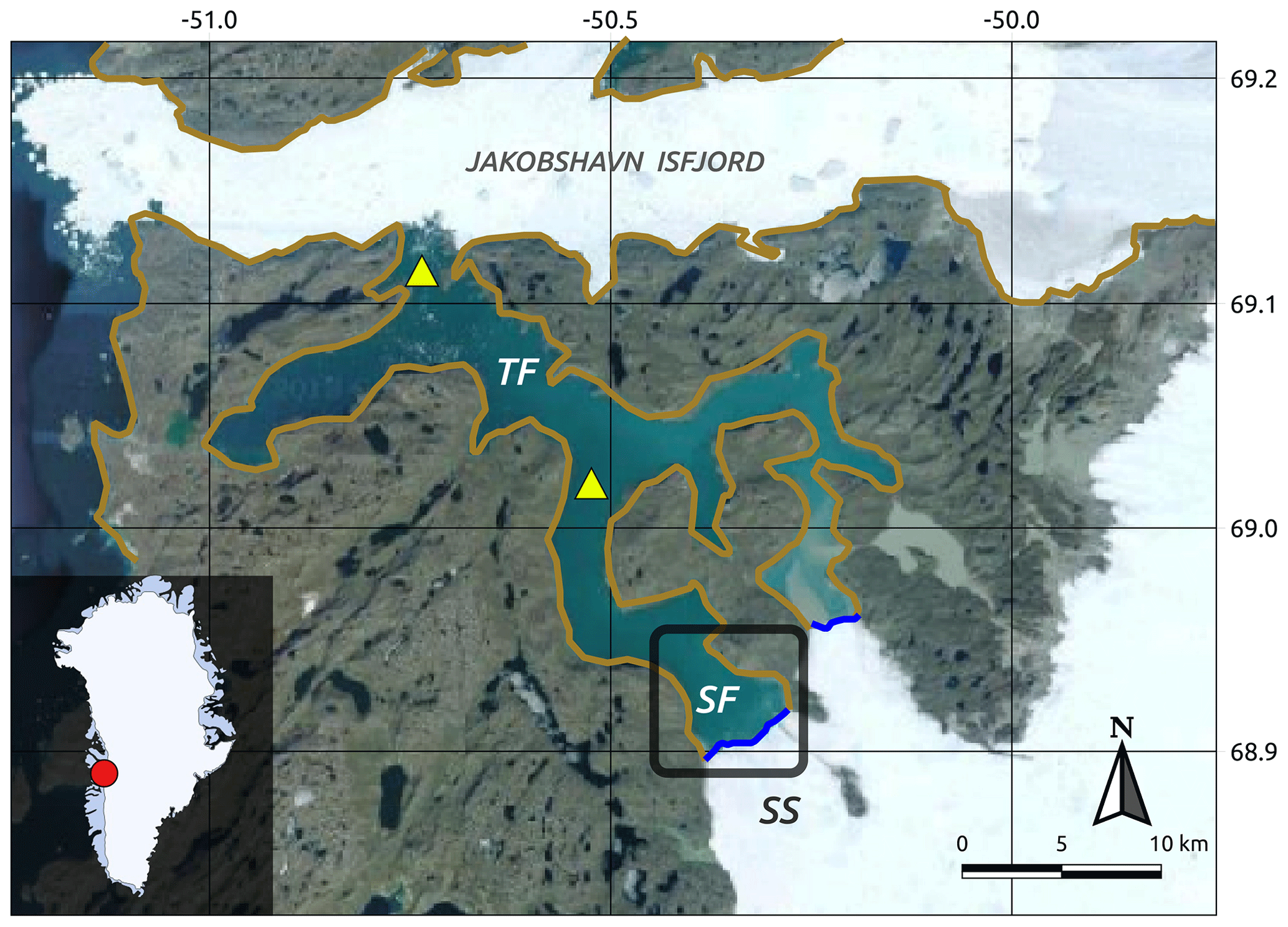
Figure 1Location map of Saqqarleq Fjord–Saqqarliup Sermia (SF–SS) system (composite image from the U.S. Geological Survey and © Google Earth, 2019). Coast lines (light brown) and glacier fronts (blue) have been superimposed. Yellow triangles indicate sill locations. The dark rectangle corresponds to the SF–SS area shown in Fig. 2. The inset shows the location in central-western Greenland.
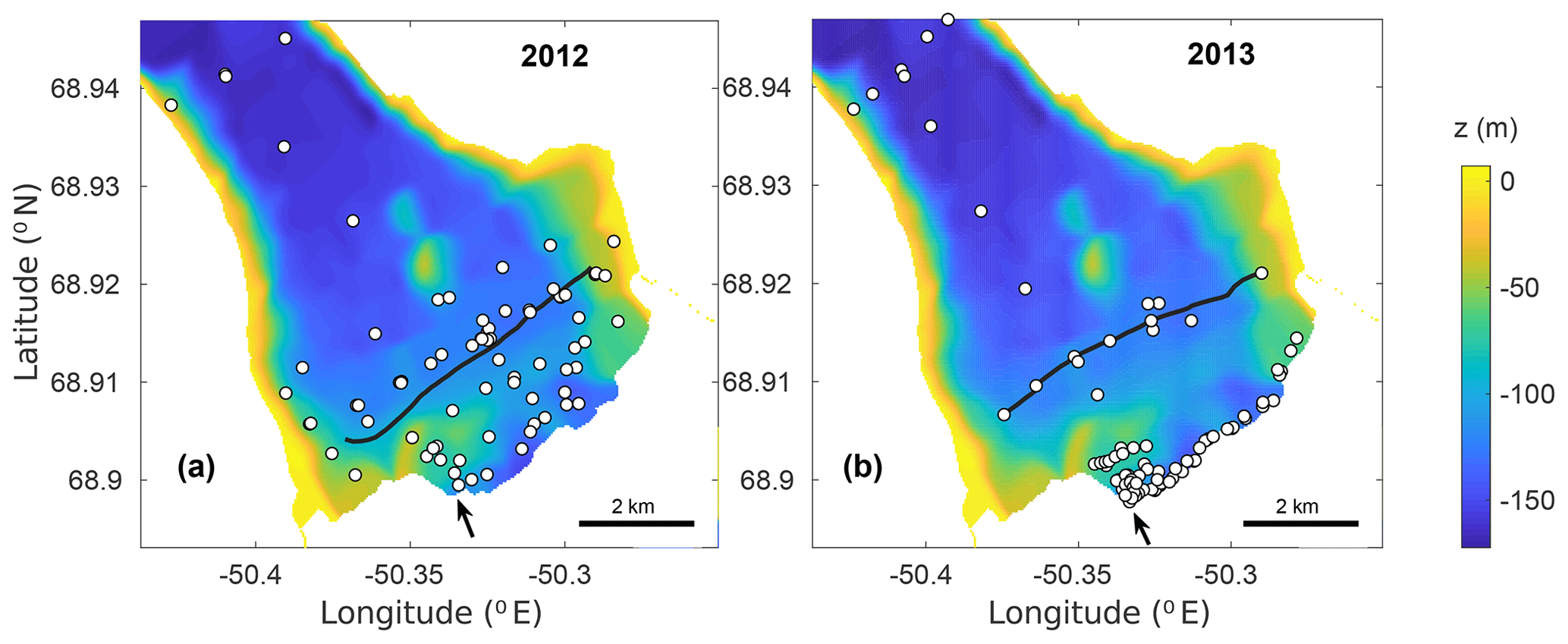
Figure 2Bathymetric map of the Saqqarleq Fjord area (dark rectangle in Fig. 1). CTD cast locations (white dots) and ADCP transects (dark lines) in 2012 (a) and 2013 (b). The location of the main plume is indicated by the black arrow.
2.1 Field data
Two field surveys were carried out in consecutive summers from 17 to 27 July 2012 and from 24 to 31 July 2013 (Mankoff et al., 2016; Slater et al., 2018; Stevens et al., 2016; Wagner et al., 2019). The glacier terminus was located approximately in the same position during the summers of 2012 and 2013 (Stevens et al., 2016), so that the geometry of the system can be considered the same in both field surveys. In 2012 (2013), a total of 90 (96) CTD (conductivity, temperature and depth) profiles were collected using an RBR XR 620 sensor that was calibrated pre-deployment and post-deployment. CTD stations were distributed along several across-fjord (terminus-parallel) and along-fjord transects (Fig. 2). The CTD profiles were collected from a small boat, and they extend from 150 m to 5 km from the glacier terminus. Temperature and salinity profiles even closer to the glacier front (and inside of the plume surface expression in 2013) were collected by deploying Sippican xCTDs (expendable CTDs) from a helicopter: 2 such profiles were obtained in 2012 and 12 in 2013. All CTD and xCTD data were depth-averaged to a resolution of 1 m. One-way ANOVA (analysis of variance) showed no significant differences between CTD and xCTD casts taken on different days (Mankoff et al., 2016), and thus we assume that properties did not change considerably within either field campaign. Temperature and conductivity values have been converted to conservative temperature (Θ) and absolute salinity (SA), respectively (IOC, SCOR and IAPSO, 2010), using the thermodynamic equation of state, TEOS-10 (McDougall and Barker, 2011).
Parallel to and at a distance of ∼1.5 km from the glacier front, water velocity surveys were performed on 20 July 2012 (DOY 202) and 26 July 2013 (DOY 207) (Fig. 2). The observations were obtained from an acoustic Doppler current profiler (ADCP, RDI 300 kHz) mounted on the small boat and binned into 4 m depth bins after removing the ship motion and corrected for local magnetic declination. ADCP data were processed using CODAS (Common Oceanographic Data Access System) from the University of Hawaii. Data were spatially interpolated by kriging to obtain the cross-sectional (terminus-parallel) contour maps.
Fjord bathymetry was obtained from the shipboard single-beam depth sounder, the shipboard ADCP and the REMUS-100 (remote environmental measuring units) autonomous underwater vehicle (AUV), as described in Stevens et al. (2016) and Wagner et al. (2019). We also make use of aerial photographs taken from the helicopter in May–June and July of 2012 and 2013 to provide a snapshot of the surface expression of the sediment-laden buoyant plumes.
2.2 Runoff estimates
Estimates for subglacial runoff from SS were determined as in Mankoff et al. (2016) and Stevens et al. (2016). Briefly, the SS catchment area was determined based on hydropotential flow routing, which is governed by SS surface and bed topography (Cuffey and Paterson, 2010; Stevens et al., 2016). Stevens et al. (2016) determined that SS has three subcatchments each draining through the terminus; in this study, we consider both the SS total catchment (Ctot) and the largest subcatchment (C1). Once these catchments have been defined, subglacial runoff for both 2012 and 2013 was estimated by summing RACMO2.3 surface melting over the catchments (van den Broeke et al., 2009). We make the common assumption that meltwater generated at the glacier surface emerges instantaneously from the glacier grounding line.
2.3 Buoyant plume model
Buoyant plume theory is a common tool for developing insight into plume dynamics and the dominant controls on their variability (e.g., Carroll et al., 2015, 2016; Cowton et al., 2016; Jenkins, 2011). The limited information we have on plume geometry suggests a truncated line plume model is the most appropriate for plumes driven by subglacial discharge at tidewater glaciers (Fried et al., 2015; Jackson et al., 2017). Therefore, in this study, we use the line plume model of Jenkins (2011) to reproduce the observed plume features and to elucidate the mechanism that suppressed the buoyant plume extent during the record 2012 melt season. We generalize the relative importance of environmental forcings by obtaining a scaling for plume vertical extent in terms of subglacial discharge flux and stratification.
2.3.1 Model description
In the plume model, the evolution of the buoyant plume properties (width, vertical velocity, temperature and salinity) along the vertical glacier face is described by four ordinary differential equations that conserve the fluxes of mass, momentum, heat and salt (the reader is directed to Jenkins, 2011, for details of the equations solved). The model is steady in time and integrated over the plume cross section, leaving the along-flow direction (i.e., z) as the only independent variable. The entrainment of ambient waters into the plume is assumed to be proportional to the vertical velocity along the plume with a constant of proportionality α. We assume a constant value of the entrainment coefficient, α=0.09, which falls within the range obtained empirically for geophysical fluid processes (Carazzo et al., 2008) and within the values used in previous studies in SF (Mankoff et al., 2016; Stevens et al., 2016). The model is closed using constant drag () coefficient, the thermodynamic equation of seawater (TEOS-10, McDougall and Barker, 2011) and three equations representing the thermodynamic equilibrium at the ice–ocean interface (Holland and Jenkins, 1999), which allows estimation of the submarine melt rate of the calving front. As boundary conditions the plume model requires profiles of the ambient fjord conditions, which are obtained from observations as described further below. Given an initial flux of subglacial discharge, assumed to have zero salinity and to be at the pressure melting point, the solution is then obtained by numerical integration.
2.3.2 Model experiments
While immersed in stratified environments, vertical plume development is finite and the plume has two characteristic plume heights (Fig. 3; List, 1982; Morton et al., 1956). The first, NBD, is reached when the plume density equals the ambient density. From this point, the plume continues upwards due to vertical momentum but slows due to the reversed buoyancy experienced above the NBD. The plume reaches MHD where the vertical velocity reaches zero (Baines, 2002; Morton et al., 1956; Slater et al., 2016). Buoyant plume theory does not capture the dynamics of waters in the plume beyond this point; however, the waters are negatively buoyant and will therefore sink as they flow away from the glacier, eventually equilibrating somewhere near the NBD (Fig. 3; e.g., Carroll et al., 2015). Thereafter, waters in the plume flow horizontally and can be treated as a jet (Bleninger and Jirka, 2004; Caufield and Woods, 1998; Jirka, 2004).
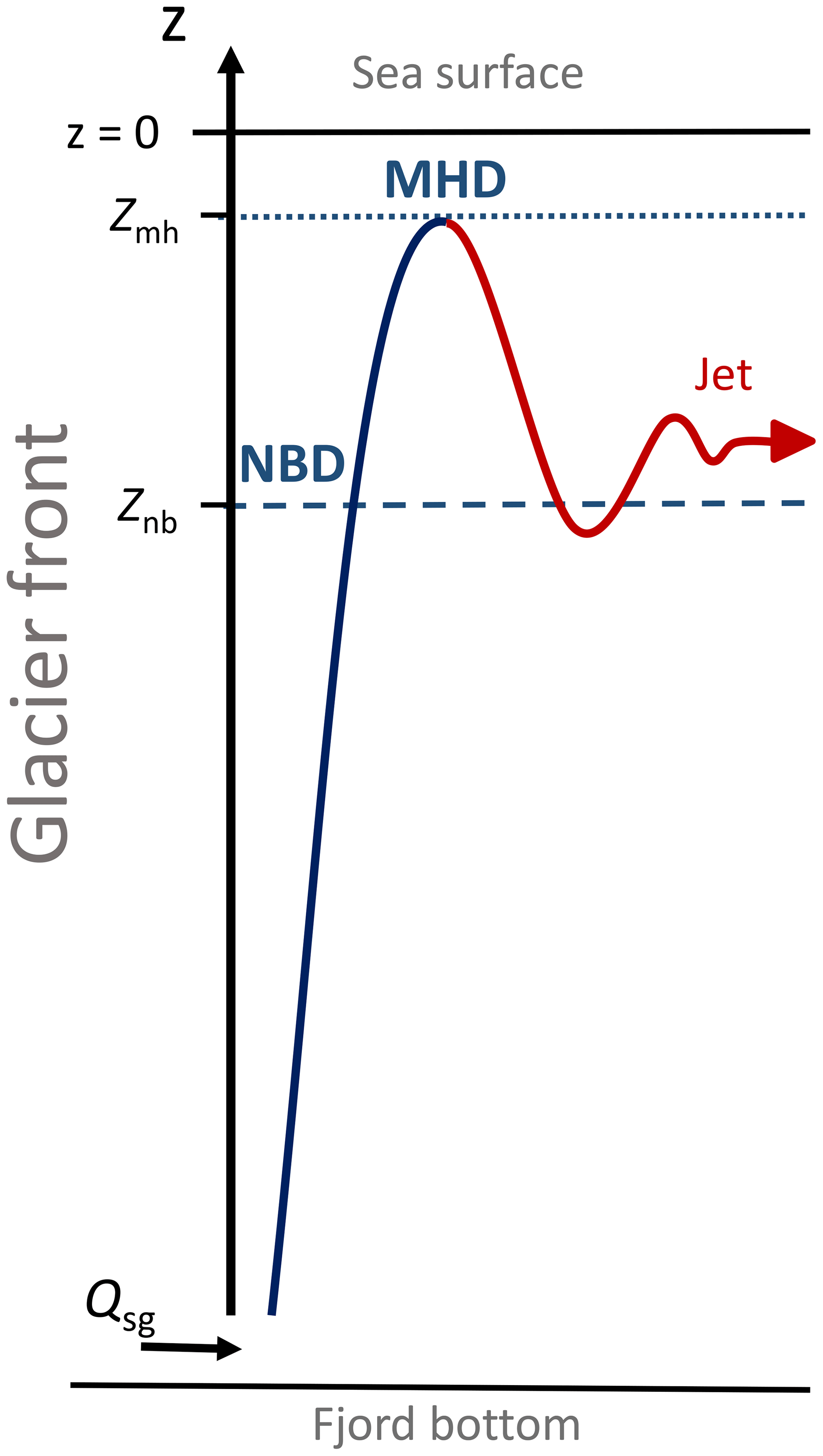
Figure 3Schematic of plume characteristic heights, i.e., neutral buoyancy depth (NBD) and maximum height depth (MHD), and the associated jet pathway. Note that the plume model does not represent plume dynamics after the maximum height is reached (red line), but it is expected that the jet will sink to a depth similar to the NBD.
To analyze the sensitivity of plume vertical extent to subglacial discharge and fjord stratification, we run the plume model for each year using ambient fjord conditions constructed from averaging all CTD casts from the given year, excluding casts from within the plume as the ambient fjord conditions are intended to represent the ambient waters through which the plume is rising. We consider a wide range of subglacial discharge fluxes (Qsg, from 10 to 400 m3 s−1, every 10 m3 s−1) and subglacial channel widths (W, from 50 to 200 m, every 10 m), though ultimately it is only the combined quantity Qsg∕W that affects the line plume model solution (Slater et al., 2016). We evaluate the model on three principal aspects. First, the fact that, according to our field observations, the plume should surface in 2013 but not in 2012. Second, we compare the modeled plume NBD with the observed depth of the jet in the water velocity measurements. Third, we compare modeled and observed plume temperature and salinity properties at the fjord surface.
2.3.3 Scalings
After evaluating the model at SF with realistic 2012 and 2013 conditions, we seek to generalize our results by investigating the scaling of plume vertical extent with subglacial discharge flux and stratification. Stratification may be quantified through the squared Brunt–Väisälä buoyancy frequency, N2, defined as follows:
where ρ is water density determined from Θ and SA at depth, ρref is the reference density, which, for our purposes, will be that at the fjord bottom, and g is the gravitational acceleration (with no geographical dependency). To find a scaling, we fit a suite of plume model results, using nonlinear least squares, to a simple curve that takes the following form:
where Z accounts for the characteristic plume height (either of NBD or MHD) in meters, A is a dimensionless constant of proportionality and a and b are the (dimensionless) powers of the scaling. N0 and Q0 are constant values of stratification and subglacial discharge, respectively, here taken to be s−2 and Q0=100 m3 s−1, and Z0 is a constant height defined in Appendix A. According to the bathymetry and CTD data (see Sect. 3), the fjord depth is set to 150 m and divided into two layers: the unstratified bottom layer (from the bottom to 100 m depth) and the linearly stratified top layer (100 m depth to the sea surface), so that N2 in the scaling (Eq. 2) is taken to be the stratification on the top layer. Given the weak impact of temperature on density, in this exercise we assume a constant temperature profile Θ (z)=1 ∘C (which is in fact close to the real conditions at Saqqarleq, except close to the surface), so that the stratification is determined solely by salinity gradient. SA of the bottom layer is held constant at 33.6 g kg−1, while the top layer is linearly stratified in salinity with a sea surface SA ranging from 33 to 24 g kg−1, which allows us to analyze stratification strengths (N2) from 2 to s−2. Runoff (Qsg) varies from 60 to 180 m3 s−1 every 20 m3 s−1. An identical procedure is used to find a scaling for the submarine melt flux, in m3 s−1, defined by the following equation:
where is the submarine melt rate, in m s−1, as calculated by the plume model. In this case the scaling takes the following form:
where N0 and Q0 are the same as for the height scaling and M0 is a constant melt rate factor defined in Appendix A.
3.1 Observations
3.1.1 Plume observations
Aerial images show that the main plume at SS was observed at the fjord surface on 1 June 2012 (Fig. 4a) but that it was not at the fjord surface once the field campaign began on 17 July 2012 (Fig. 4b, c). The plume was furthermore not seen at the fjord surface at any point during the 11 d of the 2012 field campaign. Conversely, the plume was clearly visible at the fjord surface on 23 July 2013 (Fig. 4d, e), and it was continuously at the fjord surface for the 8 d of the 2013 field campaign. The surface expression of the plume observed in 2013 extended approximately 200 m along the glacier front and 300 m into the fjord (Fig. 4d, e; Mankoff et al., 2016). Water inside the plume appeared brown due to the high sediment concentration of subglacial discharge. Despite the differing surface expression of the plume in 2012 and 2013, as described further below, we know from hydrographic and velocity measurements that the plume and the associated jet were indeed present at the same location in both years (Mankoff et al., 2016; Stevens et al., 2016).
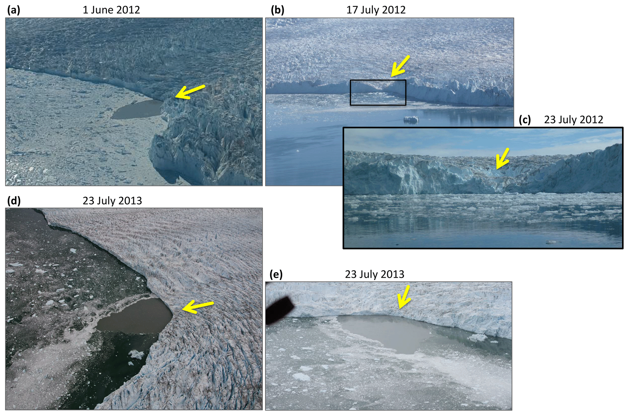
Figure 4Aerial images of the main plume at Saqqarliup–Saqqarleq front visible at the fjord surface on (a) 1 June 2012, (d) and (e) 23 July 2013 but absent on (b) 17 July 2012. Also absent was the plume on 23 July 2012, as shown in (c), a photograph taken from the boat, which covers the black rectangle in (b). The yellow arrows approximately indicate the ice flow direction in that corner of the glacier and point at the plume origin. The brown plume surface expression in (d) extends approximately 200 m along the glacier front and around 300 m into the fjord.
3.1.2 Fjord structure
CTD profiles from SF show that, in general, the fjord properties were similar in both years with a strongly stratified, warm and fresh upper 20 m layer and a more weakly stratified deeper layer (Fig. 5). The water column was substantially more stratified in 2012 than in 2013, due largely to fresher conditions in the upper 20 m but also a more moderate freshening extending to ∼100 m depth. Fjord waters in the upper 20 m were also substantially warmer in 2012 than 2013. The waters found at depth in SF are cooler than the relatively warm Atlantic Waters (AW) often found at depth in Greenlandic fjords (Straneo et al., 2012; Straneo and Cenedese, 2015). SF is relatively shallow, having a maximum depth of 230 m, and is separated from the open ocean by sills at 70 m to Tasiusaq Fjord and 125 m to Ilulissat Icefjord (Fig. 1). As such we do not see AW in Saqqarleq Fjord, instead we see cooler Ilulissat Icefjord waters (IIW, Fig. 5, Stevens et al., 2016).
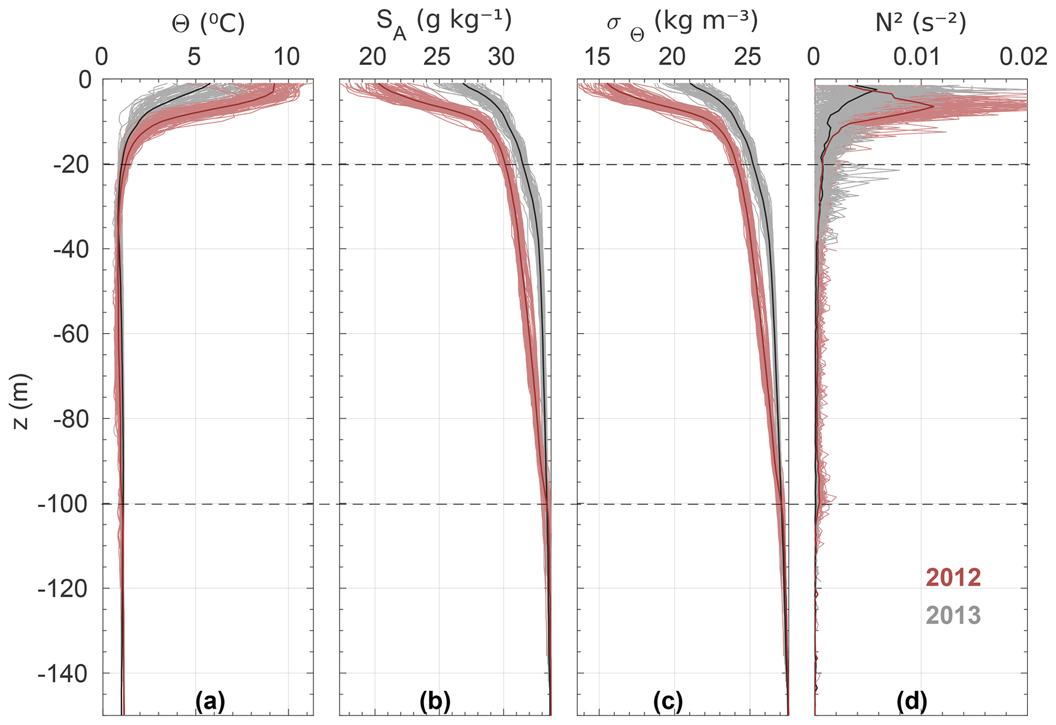
Figure 5(a) Conservative temperature, (b) absolute salinity, (c) sigma–theta (potential density – 1000 kg m−3) and (d) squared Brunt–Väisälä frequency profiles (Eq. 1) derived from CTD casts in Saqqarleq fjord during field surveys in July 2012 (red) and 2013 (grey). Averaged profiles are shown as darker lines and are used as ambient boundary conditions for the line plume model. Casts from inside the plume are not included here. Note that the water column is characterized in three layers separated by dashed horizontal lines.
To characterize differences between the years, we first divide the profiles into three layers, according to common characteristics (Fig. 5). The bottom layer, defined from the fjord bottom to −100 m, was well mixed in the vertical and had a conservative temperature around 1 ∘C and absolute salinity of ∼34.6 g kg−1. Differences observed in this layer between the 2 years are negligible. The intermediate layer, from ∼20 to 100 m depth, was also characterized by a temperature of approximately 1 ∘C and a weak salinity stratification. The salinity gradient within this layer in 2012 was double that of 2013 (−0.04 g kg−1 m−1 compared to −0.02 g kg−1 m−1). The top layer comprises the uppermost 20 m of the water column and has a strong gradient in both temperature and salinity in both years. The conditions of maximum temperature and minimum salinity occurred at the surface. In 2012, surface conditions were warmer (up to 10 ∘C) and fresher (as low as 17 g kg−1) than in 2013, and the upper layer was more strongly stratified in 2012 compared to 2013, reaching maximum values of N2>0.011 s−2 in 2012 compared to N2<0.006 s−2 in 2013 when we average over all profiles in the year (Fig. 5d).
A comparison of Θ−SA properties of the water masses (Fig. 6) again shows that the decreased salinity in 2012 relative to 2013 was distributed from the intermediate layer (σΘ of ∼24–26 kg m−3) towards the surface. The near-vertical isopycnals in Fig. 6 result from the dominant effect of salinity on water density within the ranges considered in this study. Thus, the freshening of the fjord in 2012 relative to 2013 means that middle and upper layers in 2012 were much lighter than in 2013.
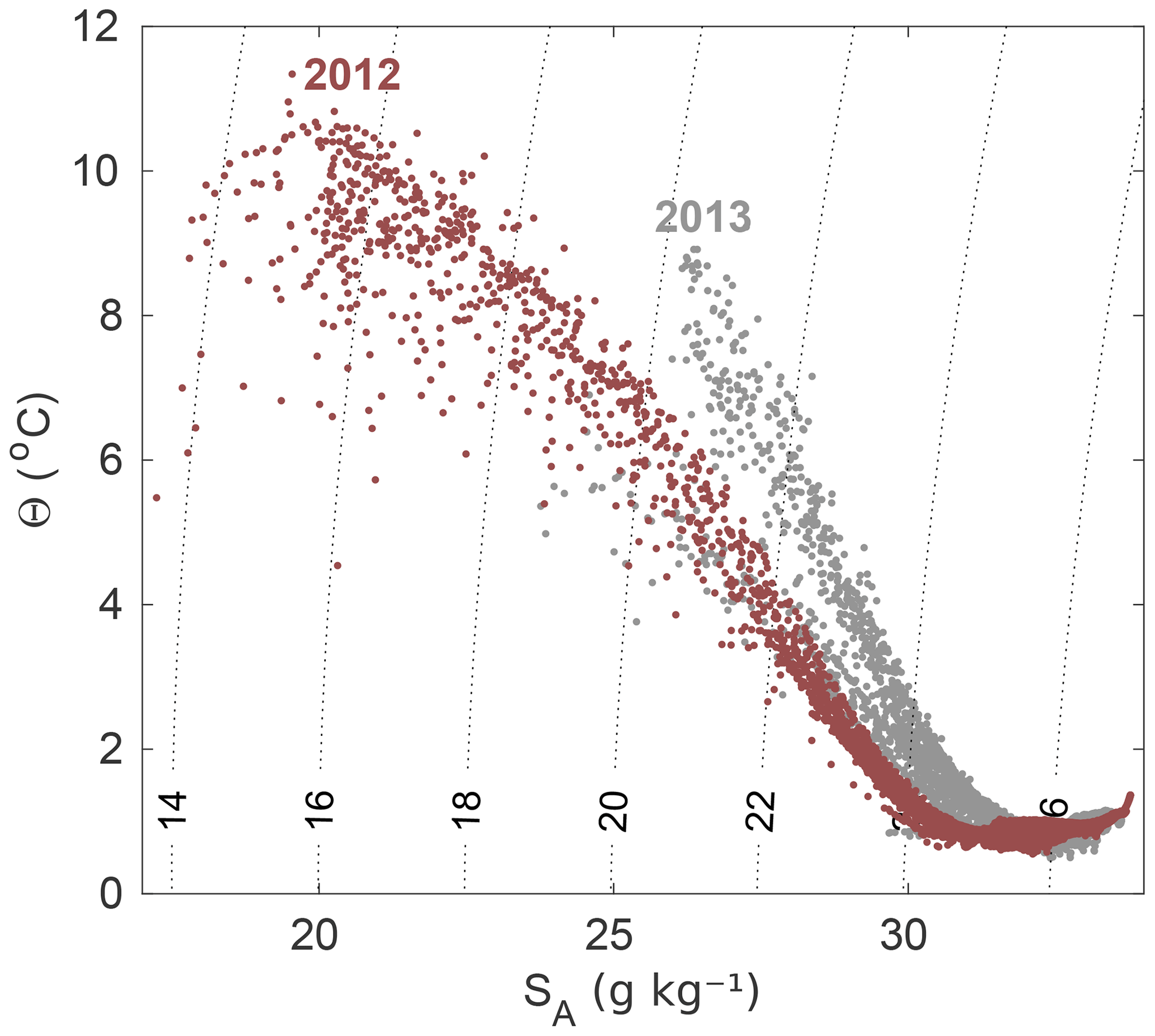
Figure 6Conservative temperature vs. absolute salinity diagram, showing the different water properties in Saqqarleq Fjord during fieldwork in July 2012 (red) and 2013 (grey). Isopycnals of sigma–theta are plotted as dotted near-vertical lines.
To quantify the additional freshwater in the inner part of the fjord (up to the SF–TF sill; see Fig. 1) in 2012 relative to 2013, we consider the depth range from z= m (sea surface) to m depth (bottom–middle layer interface). We assume the area of the inner part of the fjord to be constant in the vertical, km2, and, following Rabe et al. (2011), we calculate the volume of additional freshwater as follows:
where S2013, 2012(z) are the averaged salinity profiles for the respective years (see Fig. 5). We obtain a freshwater excess of 0.16 km3 (i.e., ∼0.16 Gt) in 2012 relative to 2013, equivalent to 4.5 m of additional freshwater per unit area of the inner fjord.
3.1.3 Plume-driven jets
Velocity data from across-fjord transects approximately ∼1.5 km from the glacier (Fig. 2) reveal the presence of a jet both in 2012 and 2013 (Fig. 7). The jet is a subsurface-intensified localized region of water flowing away from the glacier, located in the same spot in the along-front transect, oceanward of the main plume location (Figs. 2, 4 and 7). In 2012, the jet was more diffuse in the vertical, extending to 35 m depth, while in 2013 the jet was confined to the upper 20 m. Although the fjord was overall more stratified in 2012, the vertical spreading of the jet observed in 2012 could be associated with the reduced stratification surrounding the jet in 2012, s−1, compared to that of 2013, s−1. Maximum velocities of 0.35–0.4 m s−1 were found at a depth of 25 m in 2012 and 13 m in 2013. A numerical simulation of the circulation in this fjord (Slater et al., 2018) shows that these jets are the horizontal outflow from the main plume (e.g., Fig. 3). Outside of the jets, flow was generally directed towards the glacier (Fig. 7; Slater et al., 2018).
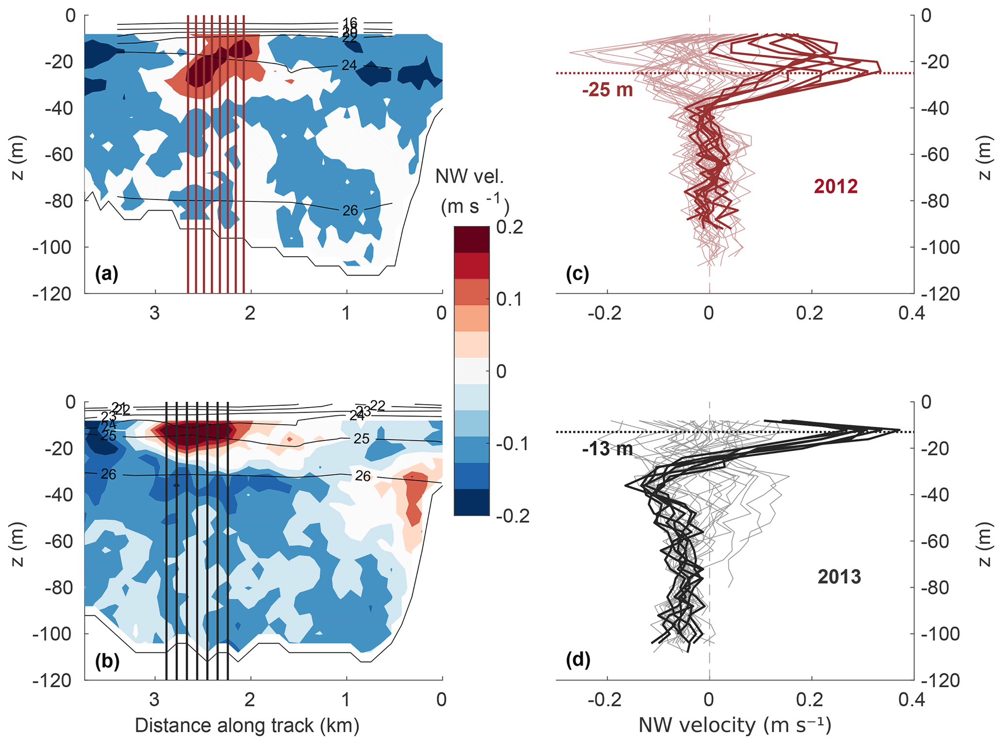
Figure 7(a, b) Fjord water velocity transects and (c, d) velocity profiles from ADCP measurements taken in 2012 (a, c) and 2013 (b, d) parallel to and at a distance of 1.5 km from the glacier front (see Fig. 2). Darker profiles in (a, b) correspond to the vertical straight lines shown in (c, d) that span the jet. The contour lines in (a) and (b) are isopycnals of sigma–theta.
The amplitude of the barotropic and baroclinic tidal currents, derived from an ADCP deployed in the middle of the fjord in summer 2012, were approximately 0.01 and 0.06 m s−1, respectively (Robert M. Sanchez, personal communication, 2020). These currents are much smaller than those observed in the jet (∼0.3 m s−1) and shown in Fig. 7, thus we do not expect that removal of the tidal velocities would significantly change the structure of the jet. The jet structure, in turn, is here used mostly to identify the water masses that are carried away from the glacier in the jet.
No local wind observations are available for the duration of the 2012 and 2013 surveys. During both surveys, however, wind conditions and sea state were largely calm and permitted surveys to be conducted from small boats and autonomous vehicles. This observation, together with the highly localized nature of the jet, support the conclusion that the jet is associated with subglacial discharge plume and is not a wind-driven feature. The numerical simulations of Slater et al. (2018), who were able to reproduce the jet with no wind forcing, also support this conclusion.
3.2 Subglacial runoff
One of the main sources of fjord freshwater is surface meltwater from the glacier's hydrological catchment basin, which enters the fjord from beneath the glacier as subglacial runoff (Fig. 8). Glacier surface melting that resulted in substantial runoff began around 1 June (DOY 150) in 2013 and around 10 d earlier in 2012. Runoff is highly variable on daily timescales but was generally greater during summer 2012 (average 122 m3 s−1) than in summer 2013 (average 92 m3 s−1), with a peak runoff in 2012 of ∼350 m3 s−1, far exceeding any value in 2013. During the time period of the fieldwork, mean daily runoff for the total catchment (major subcatchment) was 144 and 132 m3 s−1 (113 and 105 m3 s−1) in 2012 and 2013, respectively. Considering cumulative summer runoff (Fig. 8), we obtain a total of 0.98 Gt in 2012 and 0.72 Gt in 2013. That is, in 2012 there was additional freshwater runoff input of 0.26 Gt. These differences are consistent with the observation that 2012 was a record melt year in Greenland (Nghiem et al., 2012; Smith et al., 2015; Tedesco et al., 2013).

Figure 8SS runoff for the total catchment (Ctot, darker lines) and the major subcatchment (C1, lighter lines). Daily runoff estimates are shown from June to August of (a) 2012 and (b) 2013. The shaded regions comprise the field survey period (17–27 July, DOY 199-209 in 2012; 24–31 July, DOY 205-212 in 2013). The average runoff over the field survey period for C1 is shown inside the shading by a dotted line. (c) Cumulative runoff volume throughout both years, 2012 (red) and 2013 (dark grey), expressed in Gt.
3.3 Plume modeling
Analysis of the oceanographic data (Sect. 3.1) shows that a plume and the resulting jet were present during both surveys but that their characteristics were different. Specifically, (i) the plume did not reach the fjord surface in July of 2012, while it did in July 2013; (ii) fjord conditions were considerably fresher within the intermediate and top layers in 2012 than in 2013; and (iii) the plume-driven jet was found deeper in 2012 than 2013. Here, we use the line–plume model constrained by the averaged year's bulk oceanographic profiles (Fig. 5) and forced by different subglacial discharge scenarios to investigate plume behavior. The resulting modeled NBD and MHD for the main plume at SF are shown as a function of the subglacial runoff in Fig. 9. Results are shown for both 2012 and 2013, which differ in their fjord stratification as described above. For a line plume the runoff is prescribed as a runoff per unit width of grounding line (Qsg∕W); however, we also include an axis in Fig. 9 showing the absolute runoff (Qsg) assuming a line plume width of W=90 m, which was suggested by Jackson et al. (2017) to be the most appropriate for the main plume at SS.

Figure 9Characteristic plume heights obtained from the line–plume model. NBD (solid lines) and MHD (dotted lines) are obtained for 2012 (red) and 2013 (grey). Dashed horizontal lines mark the depth of the jet core observed from water velocity observations in 2012 and 2013 (Fig. 7). The top x axis represents the subglacial discharge flux applied through a channel width (W) of 90 m. The blue vertical line shows the subglacial runoff estimate (from RACMO2.3) averaged over the 5 d prior to the velocity measurements in the fjord each year (which were approximately the same: 101.7±5.7 m3 s−1 in 2012 and 101.9±13.4 m3 s−1 in 2013). The standard deviation of subglacial discharge during these 5 d is represented by the red (grey) shaded region for 2012 (2013).
We obtained deeper NBD and MHD in 2012 than 2013 for any given Qsg∕W ratio (Fig. 9), indicating that the increased stratification and freshwater content of the fjord in 2012 suppressed the vertical extent of the plume. The NBD remains subsurface for all of the Qsg∕W ratios considered here, indicating that the runoff is insufficient to generate a plume that would remain at the surface as it flowed down-fjord. The plume reaches the surface (MHD =0 m) in 2013 for Qsg∕W ratios higher than ∼0.4 m2 s−1, while the ratio has to be above ∼1.3 m2 s−1 for surfacing in 2012 (Fig. 9). Assuming a subglacial channel width of W=90 m, runoff must exceed ∼40 or ∼120 m3 s−1 for it to surface in 2013 or 2012, respectively.
We now consider whether the plume model can reproduce our observations of plume surfacing (Fig. 4 in the observations, MHD in the model) and jet depth (Fig. 7 in the observations, NBD in the model). Following Mankoff et al. (2016), we assume a subglacial runoff for each year that is averaged over the 5 d prior to the water velocity measurements that identify the jet, giving m3 s−1 in 2012 and m3 s−1 in 2013 (Figs. 8 and 9), and we assume a subglacial channel width of W=90 m in both years (Jackson et al., 2017). With these choices, as illustrated in Fig. 9 (see also Fig. 3), we find that (i) the model predicts plume surfacing in 2013 but not 2012 (consistent with observations) and that (ii) the model predicts neutral buoyancy depth that is in reasonable agreement with the observed jet depth. Given that this simple plume model is able to capture characteristics of the plume and jet in 2012 and 2013 and that the imposed subglacial runoff is almost identical between the 2 years, this confirms that differences in the plumes and jet between the 2 years are driven by differences in the stratification of the fjord.
We next consider the modeled plume temperature and salinity at NBD and MHD and compare these with observed properties within the jets flowing down fjord. Plume model properties at NBD in 2012 are characterized by SA and Θ of 30.4 g kg−1 and 0.8 ∘C, respectively, while they are 31.0 g kg−1 and 0.9 ∘C in 2013 (Fig. 10). The fresher value in 2012 is due to the greater volume of freshwater present in the fjord in 2012 (Figs. 5 and 6), which is entrained into the plume. The properties at MHD (Fig. 10) are warmer and fresher than at NBD, since the plume has by then mixed in some of the warmer and fresher waters from the upper water column (Figs. 3 and 5). The waters in the jets (∼1.5 km from the calving front) were in both years considerably warmer, fresher and lighter than at MHD in the plume (Fig. 10). The outflowing jet was also significantly fresher in 2012 than in 2013.

Figure 10Conservative temperature (Θ) and absolute salinity (SA) of Saqqarleq Fjord waters in (a) July 2012 and (b) July 2013. Light points show CTD measurements, while dark dots are xCTD measurements (closest to the plume). Conservative temperature and absolute salinity at the NBD and MHD as predicted by the plume model are shown as a yellow star and triangle, respectively. The solid blue circles represent the water properties in the core of the observed jets in Fig. 7.
Lastly, we seek to quantify the relative contribution of runoff and fjord stratification on the vertical extent of the plume in SF through a suite of plume simulations in which we systematically vary runoff and stratification. Given the very good match with observations (Fig. 9), we use the line plume model and consider a glacier front submerged in water of 150 m depth. To have better control of the stratification parameters, we approximate the observed stratification (Fig. 5), by assuming an unstratified bottom layer of 50 m and a linearly stratified upper layer with fixed thickness of 100 m representing both the middle and top layers in SF (see also Sect. 2.3.3). For simplicity, we do not separately account for the highly stratified top layer.
Figure 11 and Table 1 show the results of fitting curves of the form in Eqs. (2) and (4) to the results from the plume model. Included are both the plume extents and the vertically integrated submarine melt rate. The power law captures plume vertical extent very well (Fig. 11a), with both neutral buoyancy depth and maximum height scaling with N2 raised to the power −0.4 and runoff raised to the power 0.24. These scalings are similar to those considered in the Supplement to Slater et al. (2016), in which the equivalent exponents were −0.5 and 0.3, respectively. Slater et al. (2016), however, considered a linear stratification while here we have considered a two-layer stratification that is more representative of SF. Our results therefore show that power law scalings of the form in Eqs. (2) and (4) continue to hold in the two-layer case, provided small modifications are made to the exponents. It is also notable that the power law scalings for characteristic plume heights (Fig. 11a) perform well even in the absence of the “point source correction”; an additional term that is often added to the scaling to account for the finite size of the source of subglacial runoff (Slater et al., 2016; Straneo and Cenedese, 2015).
Table 1Results of fitting plume outputs to Eqs. (2) and (4). The plume outputs presented here are the characteristic plume heights at neutral buoyancy (Znb) and maximum extent (Zmh) and the vertically integrated submarine melt rates from the source to the neutral buoyancy height (M).
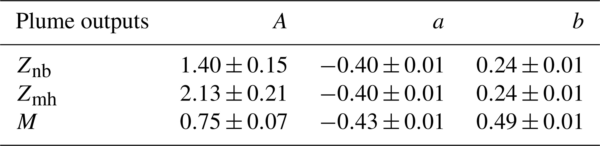
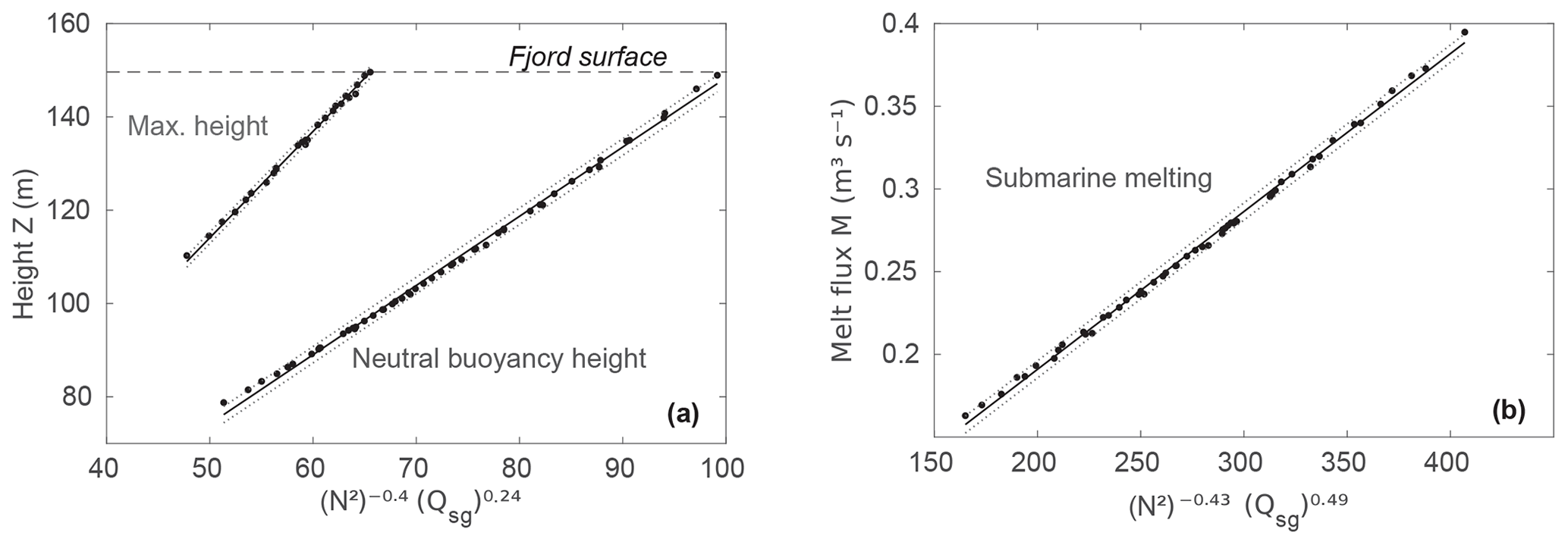
Figure 11Scaling for (a) characteristic plume heights from the source and (b) total submarine melt rates from the source to the neutral buoyancy height. Plume model results are plotted by black dots. Straight and dotted black lines represent fitting curves according to Eqs. (2) and (4) and 95 % confidence bounds, respectively. The fjord surface level has been included in panel (a) as a dashed horizontal line.
Vertically integrated submarine melt rates (i.e., the total flux of meltwater resulting from the plume) may also be expressed as a simple function of N2 and Qsg (Fig. 11b and Table 1). The stratification exponent is similar to that for the characteristic plume heights. The runoff exponent is, however, twice that of NBD and MHD, indicating that total melt rate is twice as sensitive to runoff as NBD and MHD. This reflects the fact that submarine melt rate depends on plume velocity, which also scales positively with subglacial runoff.
4.1 Impact of fjord stratification on plume dynamics in Saqqarleq Fjord
We have combined a simple plume model with oceanographic data to explain the observation of a discharge plume at SF reaching the fjord surface in 2013 but not in 2012 (Fig. 4), despite 2012 being a record surface melt year at the ice sheet scale. This is consistent with the increased stratification of the fjord in 2012 (Fig. 5), which meant that the characteristic plume heights (Fig. 3) were significantly deeper in 2012 than in 2013 (Fig. 9). The plume model also suggests that for the plume to reach the surface in 2012, the rate of subglacial discharge would have had to be 3 times that what was needed in 2013. The fact that the estimated neutral buoyancy depth is deeper in 2012 (∼25 m, Fig. 9) than the very fresh layer at the fjord surface (∼15 m, Fig. 5) suggests that it was not just the fresh surface waters that influenced plume dynamics but that the differences were also due to the stratification of the intermediate layer.
Given the observed fjord stratification and estimated subglacial discharge, the plume model shows good agreement with our plume and jet observations. The model reproduces the surfacing of the plume in 2013 but not in 2012. The simulated NBD is deeper in 2012 than in 2013 and shows reasonable agreements with the depths at which we observe jets ∼1.5 km away from the glacier (Fig. 9). Lastly, the temperature and salinity properties of the plume at the fjord surface in 2012 and 2013 lie close to those observed by expendable probes dropped close to the glacier (Fig. 10), indicating that the mixing of the plume and ambient water is reasonably captured by the model. The agreement between the model and observations is improved with respect to previous studies of Saqqarleq (Mankoff et al., 2016; Stevens et al., 2016). In our study, the modeled plume properties at NBD fall within the range of the observed water properties (Fig. 10), whereas in Stevens et al. (2016) and Mankoff et al. (2016) the modeled plume properties were consistently too light and fresh. We attribute our improved model to observation agreement to our use of a line plume model of appropriate width (Jackson et al., 2017), which, due to a larger plume surface area at depth, allows greater entrainment of denser deep waters compared with the half-conical plume model employed by Stevens et al. (2016) and Mankoff et al. (2016).
Our results also show that the observed (or modeled) plume properties, i.e., the properties observed within 150 m of the glacier face which the plume model can reproduce given the observed stratification and estimated discharge, are very different from those of the waters exported as a jet observed 1.5 km away from the glacier (Fig. 10). The fact that the properties of the jet, in both years, were considerably warmer, fresher and lighter than the observed and modeled plume properties is indicative of significant mixing with the surface waters that must occur as waters from the plume sink and flow away from the glacier. We stress that the plume model does not include this dilution, something that must be taken into account both in interpreting observations taken farther than a few 100 m away from any glacier face and/or in extrapolating plume observations and properties away from the glacier. More complex models are needed to capture this mixing and export (e.g., Slater et al., 2018).
Despite good agreement between model and observations in the plume characteristics, a number of key assumptions are worth commenting on. Our results are relatively insensitive to the assumed value of the entrainment coefficient (α). For example, allowing α to vary between 0.07 and 0.12 (which brackets the values to be found in the literature) leads to a range in NBD of 21 to 29 m in 2012 and 13 to 17 m in 2013. NBD is deeper for larger values of α because the plume entrains greater volumes of deep ambient water and is therefore denser. NBD and MHD are deeper in 2012 than in 2013 for any given value of α, confirming that stratification played a crucial role in determining plume vertical extent, and therefore our conclusions do not depend on the value of the entrainment coefficient used.
Sensitivity analyses also showed that our plume model results are insensitive to how we define the ambient fjord conditions. In principle, fjord conditions close to the glacier through which the plume is rising could differ from those a few kilometers away, meaning that the modeled characteristic plume heights (NBD and MHD) could vary depending on which CTD casts were used to define the ambient conditions for the plume model. We find, however, that in 2012 NBD only varies from 20 to 26 m when CTD casts within 150 m of the glacier or 1.5 km from the glacier are used to define the ambient fjord conditions. In 2013, the equivalent values are 13 to 15 m. MHD is similarly insensitive. Therefore, although we see substantial differences in plume dynamics between 2012 and 2013 due to differing fjord stratification, spatial variability in fjord stratification in a given year does not lead to significant differences in plume dynamics, and hence our results are not sensitive to how we define the ambient conditions in a given year.
We have assumed that meltwater from the glacier surface emerges from the grounding line instantaneously, so that estimated daily surface melting can be equated to daily subglacial discharge. Although this is a widespread assumption in glacier–fjord studies (Mankoff et al., 2016; Slater et al., 2018; Stevens et al., 2016), it is a simplification because a number of hydrological processes will act to delay this meltwater, including storage of water in supra-glacial and subglacial lakes and the finite transit time of meltwater along the ice sheet surface and bed (Fountain and Walder, 1998). This delay is likely to be significantly longer, perhaps even weeks, at the beginning of the melt season when there is still a significant snowpack and the subglacial drainage system may be inefficient (De Andrés et al., 2018; Campbell et al., 2006; Cowton et al., 2013; Schild et al., 2016). As the melt season progresses, drainage becomes more efficient, with subglacial transit velocities exceeding 1 m s−1 (Cowton et al., 2013), so that by late July when our field seasons took place, surface meltwater likely emerges from the grounding line as subglacial discharge rather rapidly, supporting our assumption. Nevertheless, uncertainty in meltwater transit time results in uncertainty in the magnitude of subglacial discharge; however, we do not believe this is sufficient to modify our conclusions.
Another source of uncertainty is the width of the subglacial channel delivering discharge into the fjord. Following Jackson et al. (2017), we have considered a channel of fixed width equal to 90 m. It is, however, expected that channel width growths with subglacial discharge due to increased melting of the channel's walls (Greenwood et al., 2016; Lliboutry, 1983). It is therefore plausible that due to the overall higher subglacial discharge in 2012 (Fig. 8), the main discharging channel at SF was larger in 2012 than 2013. A larger channel could contribute to the plume not surfacing in 2012. If the discharge was more laterally spread, the resulting plume would be less intense and would not attain the same vertical extent. The plume model nevertheless shows that the channel width would have to change by a factor of ∼3 to assume equal importance to the differing fjord stratification. Since channel theory suggests this is unlikely (e.g., Slater et al., 2015), here we have focused on the impact of fjord stratification.
Lastly, we generalized our results by using the plume model to fit a scaling between stratification (N2), subglacial discharge (Qsg), and characteristic plume heights NBD and MHD. We found that both characteristic plume heights scaled with N2 raised to the power −0.4 and Qsg raised to the power 0.24 (Fig. 11a), which are similar to those obtained by Slater et al. (2016). This means that a doubling of subglacial runoff would increase plume vertical extent (NBD and MHD) by 18 %, while a doubling of stratification would decrease plume vertical extent by 25 %. While the net impact on plume vertical extent depends on the intrinsic variability of runoff and stratification, this scaling taken together with our observations shows that stratification plays a dominant role in setting plume vertical extent. In contrast, a doubling of runoff increases total submarine melting by 40 %, while a doubling of stratification decreases total submarine melting by 26 % (Fig. 11b). For submarine melting, stratification is not dominant but still plays an important role that is worth considering in bulk submarine melt rate parameterizations.
4.2 Controls on fjord stratification
By analogy with other fjords around Greenland, water properties in SF are expected to experience strong seasonal variability as a consequence of increased glacial freshwater inputs and solar radiation during summer (Jackson et al., 2014; Schild et al., 2016; Sciascia et al., 2013; Straneo et al., 2011). We have focused largely on interannual variability by contrasting plume dynamics between July 2012 and July 2013, but in fact we also observed the plume at the fjord surface in early June 2012, when runoff is low (Figs. 4 and 8). We do not have any records of fjord properties in early June 2012, but we suspect the plume was able to surface due to a relatively unstratified water column at the beginning of the melt season. The strong stratification and the subsurface-trapped plume in late July 2012 suggests seasonal variability in fjord stratification with the fjord becoming more stratified as the melt season progresses.
The additional freshwater in the fjord in July 2012 relative to July 2013 amounts to 0.16 Gt when summed over the inner part of SF (i.e., the region shown in Fig. 2). This could be accounted for by the high subglacial discharge in 2012 which, by the end of the melt season, exceeded that from 2013 by 0.26 Gt. We do not attempt a rigorous freshwater budget here, which would account for additional freshwater sources and sinks such as the formation and melting of sea ice, melting of the calving front and icebergs, land runoff, and freshwater import and export from the fjord. Rather we suggest that due to the strong zones of recirculation observed and modeled in SF during summer (Slater et al., 2018), it is plausible that a significant fraction of the additional freshwater in 2012 remained in the inner fjord long enough to freshen the water column, leading to a stronger stratification and inhibiting the vertical extent of the plume in July 2012 compared to June 2012 and July 2013. The implication is that the glacier itself impacts the stratification of the fjord which, in turn, will have an impact on glacier–ocean exchanges and on where and how the meltwater is exported (Curry et al., 2014; Gladish et al., 2015a, b; Oliver et al., 2018; Straneo et al., 2011).
The increased freshwater content of the fjord in 2012 is not limited to the surface layer, instead extending to 100 m depth (Fig. 5). Precipitation, sea ice melting and land runoff would most strongly affect the near-surface and would have to be mixed downwards to significantly impact properties at depth. Therefore, the increased freshwater content at depth is more likely to have a glacial origin: either the melting of large deep-keeled icebergs (Enderlin et al., 2016; Moon et al., 2018), melting of the calving front itself (Slater et al., 2018; Wagner et al., 2019) or the trapping of subglacial discharge plumes below the surface (Fig. 4; Stevens et al., 2016). Considering the last point, secondary discharge channels with weaker plumes that find neutral buoyancy at greater depths (Slater et al., 2018) may play an important role in setting the seasonal fjord stratification. Equally, temporal variability in subglacial discharge of the main plume, resulting in periods where the plume reaches neutral buoyancy at depth, may drive freshening of the fjord and feedback on the dynamics of the plume. Overall we are suggesting that high surface melting through the melt season in 2012 may have freshened the fjord, driving increased fjord stratification and leading to the suppression of the plume later in the melt season.
4.3 Wider impacts of glacier–fjord coupling
In line with previous studies, our observations and supporting plume model results suggest that both subglacial discharge and fjord stratification exert a strong control on the dynamics of subglacial discharge plumes (e.g., Slater et al., 2016) with implications for melting of the glacier face and export of meltwater (Jackson et al., 2017; Mankoff et al., 2016; Stevens et al., 2016). We have also speculated that part of the differences between 2012 and 2013 in SF are due to the impact of the extreme surface melt of 2012 on the fjord raising the possibility of feedbacks between surface melt, submarine melt and export. Considering that under a high greenhouse gas emissions scenario (RCP8.5) subglacial runoff may increase by as much as a factor of 6 by the end of the century (Slater et al., 2019), it is possible that fjords will become increasingly stratified. Since stratification has proven such an important determinant of plume dynamics in this study, it is possible that despite the increased buoyancy provided by increased subglacial discharge, plumes may reach the fjord surface less often over the coming century. This may decrease our ability to observe and monitor plumes based on their surface expression, which has served as a basic but important observation for studies of fjord processes and subglacial hydrology (Schild et al., 2016; Slater et al., 2017).
From a biogeochemical perspective, a suppression of the vertical extent of plumes driven by increased fjord stratification could limit the upwelling into the photic zone of nutrients in deep water masses and from subglacial bed weathering (Cape et al., 2019; Hopwood et al., 2018; Meire et al., 2017). We acknowledge that the impact in SF in July 2012 may have been limited because, although the plume did not surface, our model suggests it was very close to the surface. Nevertheless, many of these nutrients act as a limiting factor for the primary productivity (phytoplankton) within the photic zone (Cape et al., 2019). Therefore, in contrast to some expectations (Bhatia et al., 2013), an increase in ice sheet surface melting could have a negative impact on the productivity of fjords in general. Considering that primary producers are the base of the pelagic ecosystem, a decrease in the productivity of fjord waters could negatively impact fisheries and bird populations (Arimitsu et al., 2012; Meire et al., 2017). Nevertheless, our model experiments suggest that the maximum plume height in July 2012 was only a few meters below the surface, so reduced impacts on nutrient limitations are expected to happen during July 2012. It has also been observed that the surface layer of the fjord waters (in contact with the atmosphere) is undersaturated in CO2 during the summer. Around 28 % of the uptake is attributed to the input of glacial waters and ∼72 % to primary producers (Meire et al., 2015). Therefore, a reduction of these organisms together with the subsurfacing of glacial waters could decrease the ability of the fjords to act as atmospheric CO2 sinks.
Regarding the potential implications on melting of the submerged calving front, our scalings show that stratification does indeed suppress melting of the calving front within the plume through dampening of its vertical velocity and extent. However, increased subglacial discharge has a stronger influence on melting through increasing the vertical velocity, and therefore submarine melt rates are likely to increase in response to increased ice sheet surface melting, though their vertical reach may be diminished, potentially leading to undercutting.
Lastly, stratification likely impacts on circulation more widely in the fjord, though this is beyond what we can quantify with a simple plume model. Our oceanographic observations of the jet show that due to increased stratification in 2012 compared to 2013, the jet that carries plume waters away from the glacier is deeper (Fig. 7) and fresher (Fig. 10) in 2012 than in 2013. These waters are subsequently exported from the fjord to the continental shelf where they may impact shelf properties (Luo et al., 2016), primary productivity (Arrigo et al., 2017; Oliver et al., 2018) and potentially the larger-scale ocean circulation (Böning et al., 2016; Saenko et al., 2017). Our observations suggest that in the future, increased ice sheet surface melting may stratify Greenland's fjords and modify the depth and properties of waters that are exported to the shelf. Further observations and modeling would be needed to better understand how these processes will evolve in the future.
This study began with the counterintuitive observation of a surfacing subglacial discharge plume in Saqqarleq Fjord in late July 2013 (an average melt year) but a subsurface trapped plume during late July 2012 (a record melt year). Increased subglacial discharge acts to drive a stronger plume that, in the absence of other factors, will have a greater vertical extent and probability of reaching the fjord surface. By combining oceanographic observations together with support from a plume model we have shown that the difference between the 2 years can be explained by the increased freshwater content of the fjord in 2012 relative to 2013, resulting in stronger fjord stratification and a suppression of the vertical extent of the plume. As such, seasonal and interannual variability in fjord stratification has a strong impact on the vertical extent of subglacial discharge plumes at tidewater glaciers. We suggest that the increased stratification and freshwater content of the fjord in 2012 compared to 2013 is driven by the glacier itself. In particular, strong ice sheet surface melting throughout summer 2012, delivered to the fjord as subglacial discharge, may have gradually accumulated freshwater in the fjord and increased stratification, providing a negative feedback on plume vertical extent.
Observations of the horizontal jet emanating from the plume in 2012 and 2013 show that the jet was deeper and more diffuse in 2012 and that it carried fresher and lighter water. This interannual difference is consistent with results from the plume model, in which the simulated neutral buoyancy depth of the plume proves a good estimator of the depth of the jet, and suggests once more that the driver of the observed differences is the increased stratification of the fjord in 2012. Since waters in the jet are those which will be exported from the fjord, variability in fjord stratification will impart variability on the depth and properties of waters exported from the fjord to the open ocean. We also showed, however, that the properties of waters exported from the glacier–ocean boundary in the jet approximately 1.5 km from the ice front cannot be described fully by a plume model. Instead, the jet is carrying strongly diluted plume waters through mixing with surface waters. This means that plume models or near-ice front properties are not fully representative of properties of the meltwater and ambient water mixture.
We then used the plume model to fit a scaling for plume vertical development and total submarine melting in terms of fjord stratification (N2) and subglacial discharge (Qsg). We found that plume vertical extent is proportional to , while total submarine melting is proportional to . These highlight the important role played by fjord stratification and the subglacial discharge flux in the dynamics and impacts of subglacial discharge plumes. It should be noted, however, that these scalings are based on the plume model and, as such, the quantitative details are sensitive to applied model parameters, which are poorly constrained.
Looking to the future, we are likely to see increased surface melting of the ice sheet in response to climate warming. Our results suggest that through increasing the stratification of glacial fjords, it is possible that this melting may suppress rather than promote the vertical extent of plumes and their presence at the fjord surface. This may limit our ability to monitor plumes remotely, reduce the delivery of nutrients to the photic zone, and modify the depth and properties of waters exported from the ice sheet to the ocean. Further observations and modeling are needed to better understand how the stratification of fjords and impacts on physical and biological systems may evolve in the future.
In Sects. 2.3.3 and 3.3 we define and fit scalings for plume characteristic heights and induced submarine melt rate in terms of the fjord stratification and subglacial discharge. The scaling for subglacial discharge includes a constant height Z0 defined by the following equation (see also Slater et al., 2016):
where N0 and Q0 are a constant stratification and subglacial runoff, with values given in Sect. 2.3.3, α=0.09 is the entrainment coefficient, m s−2 is the plume reduced gravity at the glacier grounding line (Slater et al., 2016), and W is the plume width, taken to be 90 m in Sect. 3.3. For the chosen parameters, Z0 takes a value 74 m in our study.
The scaling for submarine melting includes a melt rate factor M0 given by the following equation:
where cw=3974 J kg−1 ∘C−1 is the heat capacity of water, is the plume–ice drag coefficient, is the heat transfer coefficient, J kg−1 is the latent heat of melting and TF0=2.9 ∘C is the temperature of fjord waters (1 ∘C) above the in situ freezing point (−1.9 ∘C). All other variables have been previously defined. For the chosen parameters, M0 takes the value 0.37 m3 s−1 in our study.
All data used in this study are publicly available. CTD data may be found on the NSF Arctic Data Center at https://doi.org/10.18739/A2B853H78 (Straneo, 2019) and at https://data.nodc.noaa.gov/cgi-bin/iso?id=gov.noaa.nodc:0210572 (Straneo, 2020), while ADCP data may be found on NOAA-NCEI at http://data.nodc.noaa.gov/cgi-bin/iso?id=gov.noaa.nodc:0177127 (Straneo et al., 2018).
EDA, DS and FS designed the research. FS and SD collected field observations. EDA processed field and runoff data. DS provided the original model code and EDA adjusted the code to this work. EDA performed the analysis, and all the authors contributed to the discussion. EDA wrote the original text of the paper with input from all other authors.
The authors declare that they have no conflict of interest.
Eva De Andrés is supported by the Spanish Ministry of Education with the PhD studentship no. FPU14/04109. Fiamma Straneo and Donald Slater would like to acknowledge WHOI's Ocean and Climate Change Institute for funding the fieldwork and the NSF (grant no. 1418256) for funding the analysis. We would also like to thank Dan Torres, James Holte, Jeff Pietro, Clark Richards, Laura Stevens, Rebecca Jackson, Ken Mankoff, Amy Kukulya, Hanumant Singh, Robin Littlefield, Al Plueddemann, Ove Villadsen, and our colleagues from Illimanaq for their instrumental role in collecting the data and in follow-up discussions and Till Wagner for discussions about the paper.
This research has been supported by the Ministerio de Educación, Cultura y Deporte (grant no. FPU14/04109), the National Science Foundation (grant no. 1418256), the Ministerio de Economía, Industria y Competitividad, Gobierno de España (grant no. CTM2017-84441-R), and the Horizon 2020 Research and Innovation Programme (grant no. 727890).
This paper was edited by Jan De Rydt and reviewed by two anonymous referees.
Arimitsu, M. L., Piatt, J. F., Madison, E. N., Conaway, J. S., and Hillgruber, N.: Oceanographic gradients and seabird prey community dynamics in glacial fjords, Fish. Oceanogr., 21, 148–169, https://doi.org/10.1111/j.1365-2419.2012.00616.x, 2012.
Arrigo, K. R., van Dijken, G. L., Castelao, R. M., Luo, H., Rennermalm, Å. K., Tedesco, M., Mote, T. L., Oliver, H., and Yager, P. L.: Melting glaciers stimulate large summer phytoplankton blooms in southwest Greenland waters, Geophys. Res. Lett., 44, 6278–6285, https://doi.org/10.1002/2017GL073583, 2017.
Baines, P. G.: Two-dimensional plumes in stratified environments, J. Fluid Mech., 471, 315–337, https://doi.org/10.1017/S0022112002002215, 2002.
Bamber, J., van den Broeke, M., Ettema, J., Lenaerts, J., and Rignot, E.: Recent large increases in freshwater fluxes from Greenland into the North Atlantic, Geophys. Res. Lett., 39, L19501, https://doi.org/10.1029/2012GL052552, 2012.
Bhatia, M. P., Kujawinski, E. B., Das, S. B., Breier, C. F., Henderson, P. B., and Charette, M. A.: Greenland meltwater as a significant and potentially bioavailable source of iron to the ocean, Nat. Geosci., 6, 274–278, https://doi.org/10.1038/ngeo1746, 2013.
Bleninger, T. and Jirka, G.: Near- and far-field model coupling methodology for wastewater discharges, in: Environmental Hydraulics and Sustainable Water Management, Two Volume Set, vol. 1, edited by: Lee, J. H. W. and Lam, K. M., CRC Press, London, 447–453, 2004.
Böning, C. W., Behrens, E., Biastoch, A., Getzlaff, K., and Bamber, J. L.: Emerging impact of Greenland meltwater on deepwater formation in the North Atlantic Ocean, Nat. Geosci., 9, 523–527, https://doi.org/10.1038/ngeo2740, 2016.
Campbell, F. M. A., Nienow, P. W., and Purves, R. S.: Role of the supraglacial snowpack in mediating meltwater delivery to the glacier system as inferred from dye tracer investigations, Hydrol. Process., 20, 969–985, https://doi.org/10.1002/hyp.6115, 2006.
Cape, M. R., Straneo, F., Beaird, N., Bundy, R. M., and Charette, M. A.: Nutrient release to oceans from buoyancy-driven upwelling at Greenland tidewater glaciers, Nat. Geosci., 12, 34–39, https://doi.org/10.1038/s41561-018-0268-4, 2019.
Carazzo, G., Kaminski, E., and Tait, S.: On the rise of turbulent plumes: Quantitative effects of variable entrainment for submarine hydrothermal vents, terrestrial and extra terrestrial explosive volcanism, J. Geophys. Res., 113, B90201, https://doi.org/10.1029/2007JB005458, 2008.
Carroll, D., Sutherland, D. A., Shroyer, E. L., Nash, J. D., Catania, G. A., and Stearns, L. A.: Modeling Turbulent Subglacial Meltwater Plumes: Implications for Fjord-Scale Buoyancy-Driven Circulation, J. Phys. Oceanogr., 45, 2169–2185, https://doi.org/10.1175/JPO-D-15-0033.1, 2015.
Carroll, D., Sutherland, D. A., Hudson, B., Moon, T., Catania, G. A., Shroyer, E. L., Nash, J. D., Bartholomaus, T. C., Felikson, D., Stearns, L. A., Noël, B. P. Y., and van den Broeke, M. R.: The impact of glacier geometry on meltwater plume structure and submarine melt in Greenland fjords, Geophys. Res. Lett., 43, 9739–9748, https://doi.org/10.1002/2016GL070170, 2016.
Caufield, C. P. and Woods, A. W.: Turbulent gravitational convection from a point source in a non-uniformly stratified environment, J. Fluid Mech., 360, 229–248, https://doi.org/10.1017/S0022112098008623, 1998.
Cowton, T., Nienow, P., Sole, A., Wadham, J., Lis, G., Bartholomew, I., Mair, D., and Chandler, D.: Evolution of drainage system morphology at a land-terminating Greenlandic outlet glacier, J. Geophys. Res.-Earth, 118, 29–41, https://doi.org/10.1029/2012JF002540, 2013.
Cowton, T., Sole, A., Nienow, P., Slater, D., Wilton, D., and Hanna, E.: Controls on the transport of oceanic heat to Kangerdlugssuaq Glacier, East Greenland, J. Glaciol., 62, 1167–1180, https://doi.org/10.1017/jog.2016.117, 2016.
Cuffey, K. M. and Paterson, W. S. B.: The Physics of Glaciers, 4th Edn., Elsevier, Oxford, UK, 2010.
Curry, B., Lee, C. M., Petrie, B., Moritz, R. E., and Kwok, R.: Multiyear Volume, Liquid Freshwater, and Sea Ice Transports through Davis Strait, 2004–10*, J. Phys. Oceanogr., 44, 1244–1266, https://doi.org/10.1175/JPO-D-13-0177.1, 2014.
De Andrés, E., Otero, J., Navarro, F., Prominska, A., Lapazaran, J., and Walczowski, W.: A two-dimensional glacier–fjord coupled model applied to estimate submarine melt rates and front position changes of Hansbreen, Svalbard, J. Glaciol., 64, 745–758, https://doi.org/10.1017/jog.2018.61, 2018.
Enderlin, E. M., Howat, I. M., Jeong, S., Noh, M.-J., van Angelen, J. H., and van den Broeke, M. R.: An improved mass budget for the Greenland ice sheet, Geophys. Res. Lett., 41, 866–872, https://doi.org/10.1002/2013GL059010, 2014.
Enderlin, E. M., Hamilton, G. S., Straneo, F., and Sutherland, D. A.: Iceberg meltwater fluxes dominate the freshwater budget in Greenland's iceberg-congested glacial fjords, Geophys. Res. Lett., 43, 11287–11294, https://doi.org/10.1002/2016GL070718, 2016.
Fountain, A. G. and Walder, J. S.: Water flow through temperate glaciers, Rev. Geophys., 36, 299–328, https://doi.org/10.1029/97RG03579, 1998.
Fried, M. J., Catania, G. A., Bartholomaus, T. C., Duncan, D., Davis, M., Stearns, L. A., Nash, J., Shroyer, E., and Sutherland, D.: Distributed subglacial discharge drives significant submarine melt at a Greenland tidewater glacier, Geophys. Res. Lett., 42, 9328–9336, https://doi.org/10.1002/2015GL065806, 2015.
Gladish, C. V., Holland, D. M., Rosing-Asvid, A., Behrens, J. W., and Boje, J.: Oceanic Boundary Conditions for Jakobshavn Glacier. Part I: Variability and Renewal of Ilulissat Icefjord Waters, 2001–14, J. Phys. Oceanogr., 45, 3–32, https://doi.org/10.1175/JPO-D-14-0044.1, 2015a.
Gladish, C. V., Holland, D. M., and Lee, C. M.: Oceanic Boundary Conditions for Jakobshavn Glacier. Part II: Provenance and Sources of Variability of Disko Bay and Ilulissat Icefjord Waters, 1990–2011, J. Phys. Oceanogr., 45, 33–63, https://doi.org/10.1175/JPO-D-14-0045.1, 2015b.
Greenwood, S. L., Clason, C. C., Helanow, C. and Margold, M.: Theoretical, contemporary observational and palaeo-perspectives on ice sheet hydrology: Processes and products, Earth-Sci. Rev., 155, 1–27, https://doi.org/10.1016/j.earscirev.2016.01.010, 2016.
Holland, D. M. and Jenkins, A.: Modeling Thermodynamic Ice–Ocean Interactions at the Base of an Ice Shelf, J. Phys. Oceanogr., 29, 1787–1800, https://doi.org/10.1175/1520-0485(1999)029<1787:MTIOIA>2.0.CO;2, 1999.
Hopwood, M. J., Carroll, D., Browning, T. J., Meire, L., Mortensen, J., Krisch, S., and Achterberg, E. P.: Non-linear response of summertime marine productivity to increased meltwater discharge around Greenland, Nat. Commun., 9, 3256, https://doi.org/10.1038/s41467-018-05488-8, 2018.
How, P., Schild, K. M., Benn, D. I., Noormets, R., Kirchner, N., Luckman, A., Vallot, D., Hulton, N. R. J., and Borstad, C.: Calving controlled by melt-under-cutting: detailed calving styles revealed through time-lapse observations, Ann. Glaciol., 60, 20–31, https://doi.org/10.1017/aog.2018.28, 2019.
IOC, SCOR and IAPSO: The international thermodynamic equation of seawater–2010: Calculation and use of thermodynamic properties, Intergovernmental Oceanographic Commission, Manuals and Guides No. 56, UNESCO, 166 pp., 2010.
Jackson, R. H., Straneo, F., and Sutherland, D. A.: Externally forced fluctuations in ocean temperature at Greenland glaciers in non-summer months, Nat. Geosci., 7, 503–508, https://doi.org/10.1038/ngeo2186, 2014.
Jackson, R. H., Shroyer, E. L., Nash, J. D., Sutherland, D. A., Carroll, D., Fried, M. J., Catania, G. A., Bartholomaus, T. C., and Stearns, L. A.: Near-glacier surveying of a subglacial discharge plume: Implications for plume parameterizations, Geophys. Res. Lett., 44, 6886–6894, https://doi.org/10.1002/2017GL073602, 2017.
Jenkins, A.: Convection-Driven Melting near the Grounding Lines of Ice Shelves and Tidewater Glaciers, J. Phys. Oceanogr., 41, 2279–2294, https://doi.org/10.1175/JPO-D-11-03.1, 2011.
Jirka, G. H.: Integral Model for Turbulent Buoyant Jets in Unbounded Stratified Flows. Part I: Single Round Jet, Environ. Fluid Mech., 4, 1–56, https://doi.org/10.1023/A:1025583110842, 2004.
Jiskoot, H., Juhlin, D., St Pierre, H., and Citterio, M.: Tidewater glacier fluctuations in central East Greenland coastal and fjord regions (1980s–2005), Ann. Glaciol., 53, 35–44, https://doi.org/10.3189/2012AoG60A030, 2012.
Kimura, S., Holland, P. R., Jenkins, A., and Piggott, M.: The Effect of Meltwater Plumes on the Melting of a Vertical Glacier Face, J. Phys. Oceanogr., 44, 3099–3117, https://doi.org/10.1175/JPO-D-13-0219.1, 2014.
Korsun, S. and Hald, M.: Seasonal dynamics of benthic foraminifera in a glacially fed fjord of Svalbard, European Arctic, J. Foramin. Res., 30, 251–271, https://doi.org/10.2113/0300251, 2000.
List, E. J.: Turbulent Jets and Plumes, Annu. Rev. Fluid Mech., 14, 189–212, https://doi.org/10.1146/annurev.fl.14.010182.001201, 1982.
Lliboutry, L.: Modifications to the Theory of Intraglacial Waterways for the Case of Subglacial Ones, J. Glaciol., 29, 216–226, https://doi.org/10.3189/S0022143000008273, 1983.
Luckman, A., Benn, D. I., Cottier, F., Bevan, S., Nilsen, F., and Inall, M.: Calving rates at tidewater glaciers vary strongly with ocean temperature, Nat. Commun., 6, 1–7, https://doi.org/10.1038/ncomms9566, 2015.
Luo, H., Castelao, R. M., Rennermalm, A. K., Tedesco, M., Bracco, A., Yager, P. L., and Mote, T. L.: Oceanic transport of surface meltwater from the southern Greenland ice sheet, Nat. Geosci., 9, 528–532, https://doi.org/10.1038/ngeo2708, 2016.
Mankoff, K. D., Straneo, F., Cenedese, C., Das, S. B., Richards, C. G., and Singh, H.: Structure and dynamics of a subglacial discharge plume in a Greenlandic fjord, J. Geophys. Res.-Oceans, 121, 8670–8688, https://doi.org/10.1002/2016JC011764, 2016.
McDougall, T. J. and Barker, P. M.: Getting started with TEO-10 and the Gibbs Seawarer Oceanographic Toolbox, v3.05, 28 pp., edited by: SCOR/IAPSO WG127, 2011.
Meire, L., Søgaard, D. H., Mortensen, J., Meysman, F. J. R., Soetaert, K., Arendt, K. E., Juul-Pedersen, T., Blicher, M. E., and Rysgaard, S.: Glacial meltwater and primary production are drivers of strong CO2 uptake in fjord and coastal waters adjacent to the Greenland Ice Sheet, Biogeosciences, 12, 2347–2363, https://doi.org/10.5194/bg-12-2347-2015, 2015.
Meire, L., Mortensen, J., Meire, P., Juul-Pedersen, T., Sejr, M. K., Rysgaard, S., Nygaard, R., Huybrechts, P., and Meysman, F. J. R.: Marine-terminating glaciers sustain high productivity in Greenland fjords, Glob. Change Biol., 23, 5344–5357, https://doi.org/10.1111/gcb.13801, 2017.
Moon, T., Joughin, I., Smith, B., and Howat, I.: 21st-Century Evolution of Greenland Outlet Glacier Velocities, Science, 336, 576–578, https://doi.org/10.1126/science.1219985, 2012.
Moon, T., Sutherland, D. A., Carroll, D., Felikson, D., Kehrl, L., and Straneo, F.: Subsurface iceberg melt key to Greenland fjord freshwater budget, Nat. Geosci., 11, 49–54, https://doi.org/10.1038/s41561-017-0018-z, 2018.
Mortensen, J., Bendtsen, J., Motyka, R. J., Lennert, K., Truffer, M., Fahnestock, M., and Rysgaard, S.: On the seasonal freshwater stratification in the proximity of fast-flowing tidewater outlet glaciers in a sub-Arctic sill fjord, J. Geophys. Res.-Oceans, 118, 1382–1395, https://doi.org/10.1002/jgrc.20134, 2013.
Morton, B. R., Taylor, G., and Turner, J. S.: Turbulent Gravitational Convection from Maintained and Instantaneous Sources, P. R. Soc. A, 234, 1–23, https://doi.org/10.1098/rspa.1956.0011, 1956.
Motyka, R. J., Dryer, W. P., Amundson, J., Truffer, M., and Fahnestock, M.: Rapid submarine melting driven by subglacial discharge, LeConte Glacier, Alaska, Geophys. Res. Lett., 40, 5153–5158, https://doi.org/10.1002/grl.51011, 2013.
Mugford, R. I. and Dowdeswell, J. A.: Modeling glacial meltwater plume dynamics and sedimentation in high-latitude fjords, J. Geophys. Res.-Earth, 116, F01023, https://doi.org/10.1029/2010JF001735, 2011.
Nghiem, S. V., Hall, D. K., Mote, T. L., Tedesco, M., Albert, M. R., Keegan, K., Shuman, C. A., DiGirolamo, N. E., and Neumann, G.: The extreme melt across the Greenland ice sheet in 2012, Geophys. Res. Lett., 39, L20502, https://doi.org/10.1029/2012GL053611, 2012.
O'Leary, M. and Christoffersen, P.: Calving on tidewater glaciers amplified by submarine frontal melting, The Cryosphere, 7, 119–128, https://doi.org/10.5194/tc-7-119-2013, 2013.
Oliver, H., Luo, H., Castelao, R. M., van Dijken, G. L., Mattingly, K. S., Rosen, J. J., Mote, T. L., Arrigo, K. R., Rennermalm, Å. K., Tedesco, M., and Yager, P. L.: Exploring the Potential Impact of Greenland Meltwater on Stratification, Photosynthetically Active Radiation, and Primary Production in the Labrador Sea, J. Geophys. Res.-Oceans, 123, 2570–2591, https://doi.org/10.1002/2018JC013802, 2018.
Rabe, B., Karcher, M., Schauer, U., Toole, J. M., Krishfield, R. A., Pisarev, S., Kauker, F., Gerdes, R., and Kikuchi, T.: An assessment of Arctic Ocean freshwater content changes from the 1990s to the 2006–2008 period, Deep-Sea Res. Pt. I, 58, 173–185, https://doi.org/10.1016/j.dsr.2010.12.002, 2011.
Rignot, E., Velicogna, I., van den Broeke, M. R., Monaghan, A., and Lenaerts, J. T. M.: Acceleration of the contribution of the Greenland and Antarctic ice sheets to sea level rise, Geophys. Res. Lett., 38, L05503, https://doi.org/10.1029/2011GL046583, 2011.
Saenko, O. A., Yang, D., and Myers, P. G.: Response of the North Atlantic dynamic sea level and circulation to Greenland meltwater and climate change in an eddy-permitting ocean model, Clim. Dynam., 49, 2895–2910, https://doi.org/10.1007/s00382-016-3495-7, 2017.
Schild, K. M., Hawley, R. L., and Morriss, B. F.: Subglacial hydrology at Rink Isbræ, West Greenland inferred from sediment plume appearance, Ann. Glaciol., 57, 118–127, https://doi.org/10.1017/aog.2016.1, 2016.
Schild, K. M., Renshaw, C. E., Benn, D. I., Luckman, A., Hawley, R. L., How, P., Trusel, L., Cottier, F. R., Pramanik, A., and Hulton, N. R. J.: Glacier Calving Rates Due to Subglacial Discharge, Fjord Circulation, and Free Convection, J. Geophys. Res.-Earth, 123, 2189–2204, https://doi.org/10.1029/2017JF004520, 2018.
Sciascia, R., Straneo, F., Cenedese, C., and Heimbach, P.: Seasonal variability of submarine melt rate and circulation in an East Greenland fjord, J. Geophys. Res.-Oceans, 118, 2492–2506, https://doi.org/10.1002/jgrc.20142, 2013.
Shepherd, A., Ivins, E. R., A, G., Barletta, V. R., Bentley, M. J., Bettadpur, S., Briggs, K. H., Bromwich, D. H., Forsberg, R., Galin, N., Horwath, M., Jacobs, S., Joughin, I., King, M. A., Lenaerts, J. T. M., Li, J., Ligtenberg, S. R. M., Luckman, A., Luthcke, S. B., McMillan, M., Meister, R., Milne, G., Mouginot, J., Muir, A., Nicolas, J. P., Paden, J., Payne, A. J., Pritchard, H., Rignot, E., Rott, H., Sorensen, L. S., Scambos, T. A., Scheuchl, B., Schrama, E. J. O., Smith, B., Sundal, A. V., van Angelen, J. H., van de Berg, W. J., van den Broeke, M. R., Vaughan, D. G., Velicogna, I., Wahr, J., Whitehouse, P. L., Wingham, D. J., Yi, D., Young, D., and Zwally, H. J.: A Reconciled Estimate of Ice-Sheet Mass Balance, Science, 338, 1183–1189, https://doi.org/10.1126/science.1228102, 2012.
Slater, D., Nienow, P., Sole, A., Cowton, T., Mottram, R., Langen, P., and Mair, D.: Spatially distributed runoff at the grounding line of a large Greenlandic tidewater glacier inferred from plume modelling, J. Glaciol., 63, 309–323, https://doi.org/10.1017/jog.2016.139, 2017.
Slater, D. A., Nienow, P. W., Cowton, T. R., Goldberg, D. N., and Sole, A. J.: Effect of near-terminus subglacial hydrology on tidewater glacier submarine melt rates, Geophys. Res. Lett., 42, 2861–2868, https://doi.org/10.1002/2014GL062494, 2015.
Slater, D. A., Goldberg, D. N., Nienow, P. W., and Cowton, T. R.: Scalings for Submarine Melting at Tidewater Glaciers from Buoyant Plume Theory, J. Phys. Oceanogr., 46, 1839–1855, https://doi.org/10.1175/JPO-D-15-0132.1, 2016.
Slater, D. A., Straneo, F., Das, S. B., Richards, C. G., Wagner, T. J. W., and Nienow, P. W.: Localized Plumes Drive Front-Wide Ocean Melting of A Greenlandic Tidewater Glacier, Geophys. Res. Lett., 45, 12350–12358, https://doi.org/10.1029/2018GL080763, 2018.
Slater, D. A., Straneo, F., Felikson, D., Little, C. M., Goelzer, H., Fettweis, X., and Holte, J.: Estimating Greenland tidewater glacier retreat driven by submarine melting, The Cryosphere, 13, 2489–2509, https://doi.org/10.5194/tc-13-2489-2019, 2019.
Smith, L. C., Chu, V. W., Yang, K., Gleason, C. J., Pitcher, L. H., Rennermalm, A. K., Legleiter, C. J., Behar, A. E., Overstreet, B. T., Moustafa, S. E., Tedesco, M., Forster, R. R., LeWinter, A. L., Finnegan, D. C., Sheng, Y., and Balog, J.: Efficient meltwater drainage through supraglacial streams and rivers on the southwest Greenland ice sheet, P. Natl. Acad. Sci. USA, 112, 1001–1006, https://doi.org/10.1073/pnas.1413024112, 2015.
Stevens, L. A., Straneo, F., Das, S. B., Plueddemann, A. J., Kukulya, A. L., and Morlighem, M.: Linking glacially modified waters to catchment-scale subglacial discharge using autonomous underwater vehicle observations, The Cryosphere, 10, 417–432, https://doi.org/10.5194/tc-10-417-2016, 2016.
Straneo, F.: Temperature and salinity profiles adjacent to a tidewater glacier in Sarqardleq Fjord, West Greenland, collected during July 2013, Arctic Data Center, https://doi.org/10.18739/A2B853H78, 2019.
Straneo, F.: Water temperature, salinity, and velocity taken by CTD and ADCP from a small boat and remote-controlled surface vehicle from 2012-07-16 to 2012-07-25 in Sarqardleq Fjord, Greenland (NCEI Accession 0210572), NOAA National Centers for Environmental Information, Dataset, available at: https://accession.nodc.noaa.gov/0210572 (last access: 15 June 2020), 2020.
Straneo, F. and Cenedese, C.: The Dynamics of Greenland's Glacial Fjords and Their Role in Climate, Annu. Rev. Mar. Sci., 7, 89–112, https://doi.org/10.1146/annurev-marine-010213-135133, 2015.
Straneo, F., Curry, R. G., Sutherland, D. A., Hamilton, G. S., Cenedese, C., Våge, K., and Stearns, L. A.: Impact of fjord dynamics and glacial runoff on the circulation near Helheim Glacier, Nat. Geosci., 4, 322–327, https://doi.org/10.1038/ngeo1109, 2011.
Straneo, F., Sutherland, D. A., Holland, D., Gladish, C., Hamilton, G. S., Johnson, H. L., Rignot, E., Xu, Y., and Koppes, M.: Characteristics of ocean waters reaching Greenland's glaciers, Ann. Glaciol., 53, 202–210, https://doi.org/10.3189/2012AoG60A059, 2012.
Straneo, F., Richards, C., and Holte, J.: Eastward and northward components of ocean current profiles from ADCP taken from small boat in Sarqardleq Fjord adjacent to a tidewater glacier, West Greenland from 2013-07-25 to 2013-07-27 (NCEI Accession 0177127), NOAA National Centers for Environmental Information, Dataset, available at: https://accession.nodc.noaa.gov/0177127 (last access: 12 June 2020), 2018.
Tedesco, M., Fettweis, X., Mote, T., Wahr, J., Alexander, P., Box, J. E., and Wouters, B.: Evidence and analysis of 2012 Greenland records from spaceborne observations, a regional climate model and reanalysis data, The Cryosphere, 7, 615–630, https://doi.org/10.5194/tc-7-615-2013, 2013.
Vallot, D., Åström, J., Zwinger, T., Pettersson, R., Everett, A., Benn, D. I., Luckman, A., van Pelt, W. J. J., Nick, F., and Kohler, J.: Effects of undercutting and sliding on calving: a global approach applied to Kronebreen, Svalbard, The Cryosphere, 12, 609–625, https://doi.org/10.5194/tc-12-609-2018, 2018.
van den Broeke, M., Bamber, J., Ettema, J., Rignot, E., Schrama, E., van de Berg, W. J., van Meijgaard, E., Velicogna, I., and Wouters, B.: Partitioning Recent Greenland Mass Loss, Science, 326, 984–986, https://doi.org/10.1126/science.1178176, 2009.
Wagner, T. J. W., Straneo, F., Richards, C. G., Slater, D. A., Stevens, L. A., Das, S. B., and Singh, H.: Large spatial variations in the flux balance along the front of a Greenland tidewater glacier, The Cryosphere, 13, 911–925, https://doi.org/10.5194/tc-13-911-2019, 2019.
Xu, Y., Rignot, E., Fenty, I., Menemenlis, D., and Flexas, M. M.: Subaqueous melting of Store Glacier, west Greenland from three-dimensional, high-resolution numerical modeling and ocean observations, Geophys. Res. Lett., 40, 4648–4653, https://doi.org/10.1002/grl.50825, 2013.