CryoSat Ice Baseline-D validation and evolutions

The ESA Earth Explorer CryoSat-2 was launched on 8 April 2010 to monitor the precise changes in the thickness of terrestrial ice sheets and marine floating ice. To do that, CryoSat orbits the planet at an altitude of around 720 km with a retrograde orbit inclination of 92^∘ and a quasi repeat cycle of 369 d (30 d subcycle). To reach the mission goals, the CryoSat products have to meet the highest quality standards to date, achieved through continual improvements of the operational processing chains. The new CryoSat Ice Baseline-D, in operation since 27 May 2019, represents a major processor upgrade with respect to the previous Ice Baseline-C. Over land ice the new Baseline-D provides better results with respect to the previous baseline when comparing the data to a reference elevation model over the Austfonna ice cap region, improving the ascending and descending crossover statistics from 1.9 to 0.1 m. The improved processing of the star tracker measurements implemented in Baseline-D has led to a reduction in the standard deviation of the point-to-point comparison with the previous star tracker processing method implemented in Baseline-C from 3.8 to 3.7 m. Over sea ice, Baseline-D improves the quality of the retrieved heights inside and at the boundaries of the synthetic aperture radar interferometric (SARIn or SIN) acquisition mask, removing the negative freeboard pattern which is beneficial not only for freeboard retrieval but also for any application that exploits the phase information from SARIn Level 1B (L1B) products. In addition, scatter comparisons with the Beaufort Gyre Exploration Project (BGEP; https://www.whoi.edu/beaufortgyre, last access: October 2019) and Operation IceBridge (OIB; Kurtz et al., 2013) in situ measurements confirm the improvements in the Baseline-D freeboard product quality. Relative to OIB, the Baseline-D freeboard mean bias is reduced by about 8 cm, which roughly corresponds to a 60 % decrease with respect to Baseline-C. The BGEP data indicate a similar tendency with a mean draft bias lowered from 0.85 to −0.14 m. For the two in situ datasets, the root mean square deviation (RMSD) is also well reduced from 14 to 11 cm for OIB and by a factor of 2 for the BGEP. Observations over inland waters show a slight increase in the percentage of good observations in Baseline-D, generally around 5 %–10 % for most lakes. This paper provides an overview of the new Level 1 and Level 2 (L2) CryoSat Ice Baseline-D evolutions and related data quality assessment, based on results obtained from analyzing the 6-month Baseline-D test dataset released to CryoSat expert users prior to the final transfer to operations.

1 Introduction

To better understand how climate change is affecting Earth's polar regions in terms of diminishing ice cover as a consequence of global warming, there remains an urgent need to determine more precisely how the thickness of the ice is changing, both on land and floating on the sea, as also detailed in the last Intergovernmental Panel on Climate Change (IPCC) Special Report on the Ocean and Cryosphere in a Changing Climate (https://www.ipcc.ch/srocc/download-report/, last access: October 2019).

In this respect, the ESA Earth Explorer CryoSat-2 (hereafter CryoSat) monitors the changes in the thickness of marine ice floating in the polar oceans and the variations in the thickness of vast ice sheets which influence global sea levels. To achieve its primary mission objectives, the CryoSat altimeter is characterized by three operating modes, which are activated according to a geographic mode mask: (1) pulse-width-limited low-resolution mode (LRM), (2) pulse-width-limited and phase-coherent single-channel synthetic aperture radar (SAR) mode, and (3) the dual-channel pulse width and phase-coherent synthetic aperture radar interferometric (SARIn) mode.

The CryoSat data are operationally processed by ESA over both ice and ocean surfaces using two independent processors (ice and ocean), generating a range of operational products with specific latencies. The ice processor generates Level 1B (L1B) and Level 2 (L2) offline products typically 30 d after data acquisition for the three instrument modes, LRM, SAR and SARIn. The ice products are currently generated with the Ice Baseline-D processors and have been since 27 May 2019. The main outputs of the L2 Ice processing chain are the radar freeboard estimates and the difference in height between ice floes and adjacent waters as well as ice sheet elevations, tracking changes in ice thickness. In addition, near-real-time (NRT) products are also generated with a latency of 2–3 h after sensing to support forecasting services. Details on the previous historic CryoSat Ice processing chain and main L1B and L2 processing steps are reported in Bouffard et al. (2018b). CryoSat Ocean products are instead generated with the Baseline-C CryoSat Ocean Processor (more details in Bouffard et al., 2018a). An overview of the current CryoSat data products is reported in Fig. 1. The description and format of each of the products is available in the product format description documents (available at https://earth.esa.int/web/guest/missions/esa-operational-eo-missions/cryosat, last access: October 2019).

Figure 1 CryoSat data products overview. Map data ©2019 Google.

In order to achieve the highest quality of data products and meet mission requirements, the CryoSat Ice and Ocean processing chains are periodically updated. Processing algorithms and associated product content are regularly improved based on recommendations from the scientific community, expert support laboratories, quality control centers and validation campaigns. In this regard, the new CryoSat Ice Baseline-D processors have been developed and tested. An Ice Baseline-D test dataset (TDS) covering three different time periods (September–November 2013, February–April 2014 and April 2016 (only SARIn)) was made available to the CryoSat Quality Working Group (QWG) and scientific experts in order to opportunely validate and check the quality of the new products. This paper provides an overview of the CryoSat Ice Baseline-D evolutions of the processing algorithms and focuses on the in-depth validation performed on the TDS over land ice, sea ice and inland waters. The transfer to operations of the new CryoSat Ice Baseline-D processors was performed on 27 May 2019, and a complete mission data reprocessing is ongoing in order to provide users with homogeneous and coherent CryoSat Ice products for proper data exploitation and analysis.

The paper is structured as follows. Section 2 provides an extensive analysis of the major evolutions included in Baseline-D separated into L1B and L2 processing stages, describing the improvements that have been implemented and included in the new baseline version. Section 3 describes, based on the analysis of the 6-month TDS provided by ESA, the main validation results in different domains such as land ice, sea ice and inland waters. Section 4 reports the conclusions.

2 CryoSat Ice Baseline-D evolutions

The new Ice Baseline-D processors were approved and transferred to operation on 27 May 2019. The CryoSat Ice Baseline-D processor generates Level 1B and Level 2 Ice products from Level 0 LRM, SAR and SARIn products. These products are primarily designed for the study of land ice and sea ice, although they are also relevant and useful to a wide range of additional applications. Level 1B data consist, essentially, of an echo for each point along the ground track of the satellite. In all three modes, the data consist of multilooked echoes at a rate of approximately 20 Hz. Level 2 products instead are considered to be most suitable for users, as they contain surface height measurements fully corrected for instrumental effects, propagation delays, measurement geometry, and additional geophysical effects such as atmospheric and tidal effects. In the L2 products, the value of each geophysical correction provided is the value applied to the corrected surface height. Sea level anomalies and radar freeboard data are also included in the CryoSat Level 2 data products. A complete list of the evolutions and changes implemented in Baseline-D can be found in the technical note available at https://earth.esa.int/documents/10174/125272/CryoSat-Baseline-D-Evolutions (last access: November 2019), while a concise overview of the CryoSat L1B and L2 ice products is available at https://earth.esa.int/documents/10174/125272/CryoSat-Baseline-D-Product-Handbook (last access: February 2020). This revision of the document has been released to accompany the delivery of Baseline-D CryoSat products. Details about CryoSat and the main changes are described below separated into the L1B and L2 processing stages.

2.1 Ice Baseline-D L1B evolutions

Prior to Baseline-D, the Ice Baseline-C processors were installed on the operational and reprocessing platforms and Baseline-C L1B products were produced and distributed to users from 1 April 2015 (Scagliola and Fornari, 2015). During this period some issues were identified, and the scientific community suggested a series of evolutions that have been taken into consideration when updating the L1B processors for Baseline-D. L1B products are now generated using the new Baseline-D L1B processors, in which software issues have been fixed and new processing algorithms have been implemented (for more details refer to the Baseline-D product evolutions document available at https://earth.esa.int/documents/10174/125272/CryoSat-Baseline-D-Evolutions, last access: November 2019). One of the main quality improvements implemented in Baseline-D is the migration from Earth Explorer format (EEF) to Network Common Data Form (NetCDF). In addition, in Baseline-D the phase information available in the CryoSat SARIn acquisition mode is now used to reduce the uncertainty affecting sea ice freeboard retrievals (Armitage et al., 2014; Di Bella et al., 2018). The previous Baseline-C has shown large negative freeboard estimates at the boundary of the SARIn acquisition mask, caused by a bad phase difference calibration (see Sect. 3.3.2). In Baseline-D the accuracy of the phase difference has been improved as well as the quality of the freeboard at the SARIn boundaries, reducing drastically the percentage of negative retrievals from 25.8 % to 0.8 % (Di Bella et al., 2019). In SAR altimetry processing, after the beam-forming process, stacks are formed. A stack is the collection of all the beams that have illuminated the same Doppler cell (Raney, 1998). In Baseline-D, two additional stack characterization parameters (also known as beam behavior parameters) have been added to the SAR and SARIn L1B products: the stack peakiness and the position of the center of the Gaussian function that fits the range-integrated power of the single-look echoes within a stack, as a function of the look angle. The stack peakiness (Passaro et al., 2018) can be useful to improving the sea ice discrimination and the position of the center of the Gaussian function that fits the range-integrated power of the single-look echoes within a stack as a function of the look angle (Scagliola et al., 2015). In radar altimetry, the window delay refers to the two-way time between the pulse emission and the reference point at the center of the range window. The window delay in Baseline-D L1B products now compensates for the ultra-stable oscillator (USO) correction, which is the deviation of the frequency clock of the USO from the nominal frequency. The L1B users no longer need to apply this correction. In addition, the mispointing angle accuracy was improved by considering a proper correction for the aberration of light when the data from star trackers are processed on the ground. In fact, the star trackers compute the satellite orientation in an inertial reference frame starting from a comparison of the stars in their field of view with an onboard catalogue; therefore the aberration of light needs to be compensated for on the ground to give accurate information about the satellite attitude (more details in Scagliola et al., 2018).

Table 1 Major Baseline-D evolutions.

2.2 Ice Baseline-D L2 evolutions

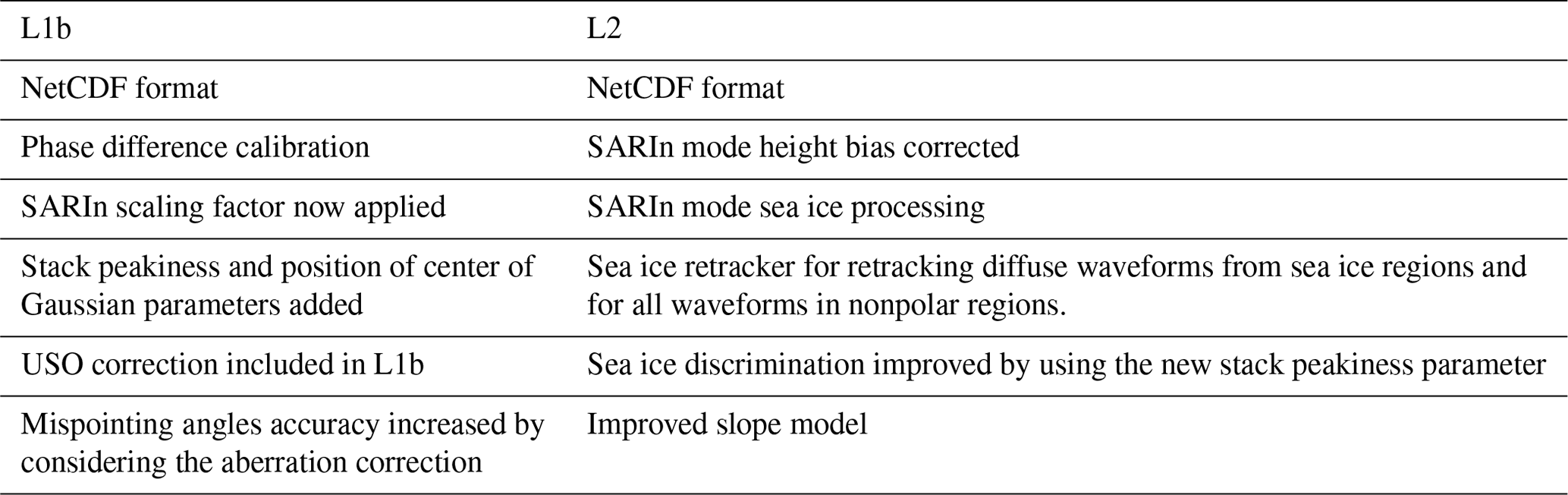
The Baseline-D update to the CryoSat L2 processing fixes a number of anomalies and introduces several processing algorithm improvements, as described in https://earth.esa.int/documents/10174/125272/CryoSat-Baseline-D-Evolutions (last access: November 2019). In addition to corrections and improvements, the L2 products are now generated in netCDF format and contain all previous parameters as well as some new ones. For example, in previous baselines, the sea ice freeboard processing was restricted to SAR mode regions, resulting in large gaps in coverage around the coast and in other regions of the Arctic operating in SARIn. In Baseline-D, the sea ice parameters are also computed over these regions. The retrieved height value is still that from the SARIn-mode-specific retracking (phase has been used to relocate the height measurement across track), but new fields have been added to contain the sea-ice-processing height result, and freeboard and sea level anomalies are now computed in SARIn mode (previously they were computed in SAR mode only). In addition, a new threshold first-maximum retracker is used for retracking diffuse waveforms from sea ice regions and all waveforms in nonpolar regions (more details in the CryoSat L2 Design Summary Document available at https://earth.esa.int/documents/10174/125272/CryoSat-L2-Design-Summary-Document, last access: January 2020). Retracking is the process whereby the initial range estimate in the L1B data is corrected for the deviation in the first echo return within the waveform from the reference position. Over sea ice, the discrimination algorithm used to determine if individual waveforms represent sea ice floes, leads in the sea ice or ice-free ocean has been improved with the implementation of a new discrimination metric based on sea ice concentration, waveform peakiness and standard deviation of the stack of waveforms as metrics, in addition to peakiness of the stack (see Sect. 3.3.1). This method improves the capability of the algorithm to reject waveforms contaminated by off-nadir specular reflections (as described in https://earth.esa.int/documents/10174/125272/CryoSat-L2-Design-Summary-Document, last access: January 2020). Some tuning of the thresholds for the other metrics has also been performed, based on analysis of the test datasets. For the land ice domain, new slope models have been generated, using the digital elevation models (DEMs) of Antarctica and Greenland described in Helm et al. (2014). These models were created with more recently acquired data and therefore better represent the slope of the surface during the period of the CryoSat mission. The DEMs were sampled at a high resolution to derive the surface slope correction. Lastly, several improvements have been made to the contents of the L2 products. The surface-type mask model used to discriminate different types of targets has been updated (as described in the Baseline-D product handbook available at https://earth.esa.int/documents/10174/125272/CryoSat-Baseline-D-Product-Handbook, last access: February 2020). Variables have been added to the netCDF to explicitly cross-reference the 1 and 20 Hz data. Finally, the retracker-corrected range to the surface has been added to the product. Table 1 summarizes the major differences between Baseline-D and Baseline-C.

3 CryoSat Ice Baseline-D validation of test dataset results

3.1 Data quality – Ice Baseline-D test data verification by IDEAS+

All CryoSat data products are routinely monitored for quality control by the ESA ESRIN (European Space Research INstitute) Sensor Performance, Products and Algorithms (SPPA) office with the support of the Instrument Data quality Evaluation and Analysis Service (IDEAS+). In preparation for the Ice Baseline-D, IDEAS+ performed quality control (QC) checks on test data generated with the new Ice Baseline-D processors (IPF1 vN1.0 and IPF2 vN1.0). For testing and validation purposes a 6-month TDS was generated at ESA in a dedicated processing environment for two periods: September–November 2013 and February–April 2014. IDEAS+ performed QC of a 10 d sample of L1B and L2 data to assess data quality and check for major anomalies. Following these QC checks, this 6-month TDS was made available to the CryoSat QWG for more detailed scientific analysis.

The content of the product header files (HDR format) was checked to confirm that all dataset descriptors (DSDs) were present and correct and all header fields were correctly filled. Similarly, the global-attributes section of the netCDF has been checked to ensure data files were consistent and complete. The CryoSat data products contain many data flags which provide information and warnings about any inconsistencies present in the data products. These flags have been checked for any unexpected values that may indicate processing anomalies, and all external geophysical corrections were checked to ensure that they were computed correctly. Some minor unexpected changes to the configuration of particular flags were observed as well as the incorrect scaling of the altimeter wind speed values. These minor issues have been resolved in the final Baseline-D release, which has been put into operation.

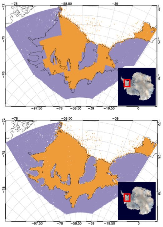
Figure 2 Surface-type mask shown for the Filchner–Ronne ice shelf area (ice shelf in orange, ice sheet in blue). Upper panel: Baseline-C; lower panel: Baseline-D. Map data ©NASA/Dave Pape.

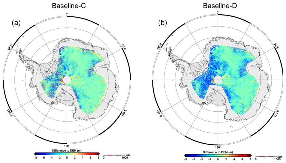
Figure 3 Differences in slope-corrected LRM data to reference DEM (REMA, Howat et al., 2019) in Antarctica. (a) Baseline-C REMA: $+\mathrm{0.13}\pm \mathrm{1.2}$ m; (b) Baseline-D REMA: $-\mathrm{0.11}\pm \mathrm{1.11}$ m.

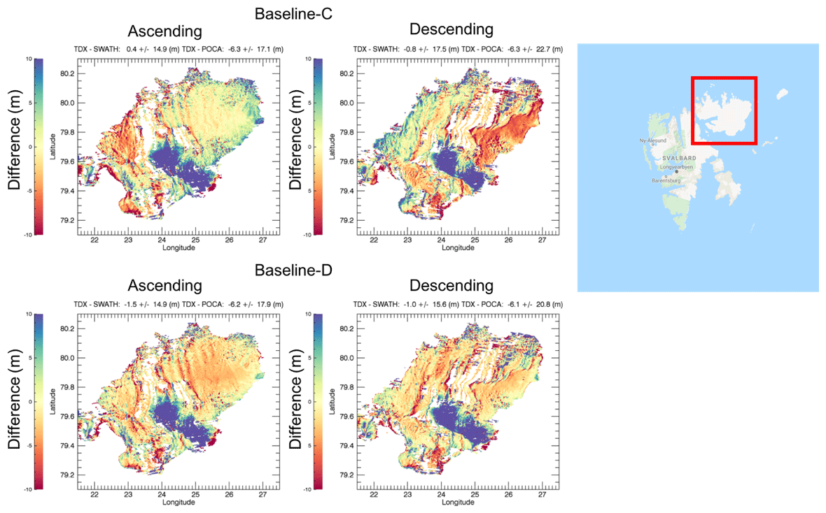
Figure 4 Differences to reference elevation model derived from TanDEM-X data from 2012 across the Austfonna ice cap. Upper left: ascending Baseline-C; upper right: descending Baseline-C; lower left: ascending Baseline-D; lower right: descending Baseline-D. Map data ©2019 Google.

Figure 5 Difference in elevation between ascending and descending swath data at crossovers across Austfonna ice cap. (a, b) Baseline-C + statistics. (c, d) Baseline-D + statistics.

3.2 Land ice

3.2.1 Impact of algorithm evolution on land ice products

CryoSat L1B and L2 products generated using the Baseline-C processors are the primary input to obtain elevation change time series of the large ice sheets. As those time series are the primary dataset to obtain ice-sheet-wide mass balance and therefore the contribution to sea level change, a consistent high-quality CryoSat L1B–L2 product is essential. To derive mass balance estimates the Alfred Wegener Institute (AWI) processing chain was used, introduced by Helm et al. (2014), including TFMRA (threshold first-maximum retracker algorithm) retracking and the refined slope correction (Roemer et al., 2007) for LRM as well as an interferometric processing using phase and coherence for the SARIn mode L1B data products. In addition, several other groups rely on high-quality L1B and L2 data products to generate time series of elevation and mass change (e.g., Nilsson et al., 2015; Simonsen et al., 2017; McMillan et al., 2014; Schroeder et al., 2019). Next to the conventional along-track processing, the swath mode has been developed and explored by several groups (Gray et al., 2013; Gourmelen et al., 2017). It has been demonstrated that swath products can be used to estimate basal melt rates of ice shelves or high-resolution elevation change time series within the steep margins of the Greenland ice sheet or Arctic ice caps (Gourmelen et al., 2017). However, a small attitude angle error interpreted as a mispointing error has been observed using Baseline-C products, which is critical for the accuracy of the derived swath mode products. Bouffard et al. (2018b) presented an attitude correction to be applied to Baseline-C products, which should help to reduce this uncertainty. This has been implemented in Baseline-D, where a new star tracker processor was developed to create files containing the most appropriate star tracker data. In addition, new fields were added to the L1B products to include the antenna bench angles (roll, pitch and yaw), and the sign conventions of these fields were updated. To estimate the impact of the algorithm evolution of the CryoSat Ice processor to Baseline-D on land ice data records, L2-type products for Baseline-C and Baseline-D were computed using the AWI processing chain. In addition, a Level 2 in-depth (L2I; https://earth.esa.int/documents/10174/125272/CryoSat-Baseline-D-Product-Handbook, last access: February 2020) product retracker and slope corrections were implemented in the individual datasets to be compared. In a first instance single tracks crossing the Antarctic ice sheet were compared on a point to point basis for all of the individual parameters included in the L1B and L2I products. Most of the parameters were found to show close agreement; however a constant offset was found for σ₀ for all of the implemented LRM L2 retrackers (https://earth.esa.int/documents/10174/125272/CryoSat-Baseline-D-Product-Handbook, last access: February 2020): 0.6, 0.63 and 0.65 dB for Ocean, Ice1 and Ice2 retracker, respectively. The mentioned offsets need to be considered as long as both baselines are used in combination to estimate elevation change time series, as some groups incorporate a σ₀ correlated correction (Simonsen and Sørensen, 2017; Schröder et al., 2019). A new surface-type mask has been implemented in Baseline-D, significantly improving resolution in the ice shelf area as shown in Fig. 2 for the Filchner–Ronne ice shelf. The Level 2 products contain a flag word, provided at a 1 Hz resolution, to classify the surface-type at nadir. This classification is derived using a four-state surface identification grid, computed from a static digital terrain model 2000 (DTM2000) file provided by an auxiliary file to the processing chain.

Now, this mask can be applied to differentiate between floating and grounded ice. In addition, a new slope model for Antarctica, which is based on the elevation model of Helm et al. (2014), is implemented in Baseline-D. This slightly changes the LRM slope-corrected elevation as is demonstrated for the Antarctica region in Fig. 3.

Differences between slope-corrected elevation and an independent Antarctic elevation model (REMA; Howat et al., 2019) are shown for both baselines. The differences vary spatially, and the overall mean differences changed from +0.13 to −0.11 m. This needs to be considered when estimating time series using data of both baselines, until the full mission reprocessing is finished. The attitude information for SARIn, such as roll, pitch and yaw were updated for Baseline-D, incorporating the correction found by Scagliola at al. (2018b). The correction is as expected and agrees with the auxiliary product already delivered by ESA. This has a negligible effect for SARIn point-of-closest-approach (POCA) elevations; however it offers major improvements for swath-processed data as shown in Figs. 4 and 5. Figure 4 subpanels show the difference in swath processed data for ascending and descending tracks, respectively, to a reference elevation model derived from TanDEM-X data from 2012 for the Austfonna icecap. The large positive anomaly (blue area in Fig. 4) is a known glacier surge event (McMillan et al., 2014). The negative anomaly observed by descending tracks in the eastern part and the discrepancy between ascending and descending tracks in the western part in Baseline-C are reduced. More clearly, Fig. 5 shows this improvement in the crossover statistics. With the upcoming Baseline-D, a correction term as suggested by Gray et al. (2017) is not needed anymore and might not be appropriate as a static correction to Baseline-C, as the angle correction is variable in space and time.

3.2.2 Baseline-D SARIn swath data over Antarctica

Standard radar altimetry relies on the determination of the point of closest approach (POCA), sampling a single elevation beneath the satellite. Using the CryoSat interferometric mode (SARIn), it is possible to resolve more than just the elevation at the POCA. If the ground terrain slope is only a few degrees, the CryoSat altimeter operates in a manner such that the interferometric phase of the altimeter echoes may be unwrapped to produce a wide swath of elevation measurements across the satellite ground track beyond the POCA. Swath processing also provides a near-continuous elevation field, making it possible to form digital elevation models and to map rates of surface elevation change at a true resolution of 500 m, an order of magnitude finer than is the current state of the art for the continental ice sheets (Gourmelen et al., 2018). To assess the performance of swath data derived from Baseline-C and Baseline-D CryoSat L1B data, a point-to-point comparison was performed over the Siple Dome, Antarctica. This comparison gave a measure of the precision of swath elevation measurement and allowed for a comparison of each baseline. The Siple Dome region has been chosen as it is a relatively stable area with large areas of constant sloping terrain, ensuring a high sampling density of swath data.

The Baseline-D TDS from February to April 2014 and the Baseline-C data from the same time period were used in this assessment. Baseline-C data were used with both the original star tracker measurements and revised measurements provided by ESA. These were supplied as a result of an incorrect mispointing angle for the aberration of light being implemented in Baseline-C, which led to an error in the calculation of the roll of the satellite. Any error in the roll will result in an error in the geolocation and derived height, and this was shown to decrease the performance of swath measurements (Gray et al., 2017). Swath data were processed following Gray et al. (2013), with a minimum coherence and power threshold of 0.9 and −180 dB, respectively. For the point-to-point comparison, the closest individual swath elevation measurement from a different satellite pass was used. A comparison was only made if the maximum distance between the two geolocated elevation measurements was below 30 m. Overall 157 000 points were compared at an average distance of 19 m. As the points compared were distributed over sloping terrain, any difference in position led to an additional error, for example a horizontal offset of 19 m over a 0.5^∘ slope led to a vertical offset of ∼ 0.17 m which is included in all comparisons. The standard deviation between the point-to-point comparison for Baseline-C with the original (Fig. 6a) and the revised (Fig. 6b) star tracker measurements was 4.2 and 3.8 m, respectively, showing that correcting for the mispointing angle for aberration of light error significantly improves the precision of swath measurements, while the standard deviation of the point-to-point comparison for Baseline-D was 3.7 m, showing a slight improvement compared to Baseline-C, which can be attributed to improved processing of the star tracker measurements documented in Baseline-D.

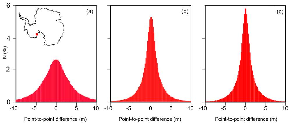
Figure 6 Point-to-point comparison of swath data over the Siple Dome (red box in map insert) for (a) Baseline-C with original star tracker measurements (b) Baseline-C with revised star tracker measurements and (c) Baseline-D.

3.2.3 SARIn validation at Austfonna, Svalbard

The southeastern basin of the Austfonna ice cap, Svalbard, began surging in 2012 (Dunse et al., 2012, 2015). The surge resulted in a heavily crevassed surface of the basin, creating a challenging surface topography for radar altimetry. CryoSat operates in SARIn mode over the Austfonna ice cap, and due to the complex surface, the ice cap has been chosen as a primary validation site for the CryoSat mission in the ESA CryoSat Validation Experiment (CryoVEx) and the ESA CryoVal Land Ice (LI) projects. Traditional airborne validation campaigns for satellite radar altimetry have targeted satellite underflights as close to the satellite nadir as possible. This approach is favorable when surveying a flat surface; however, a sloping surface will induce an off-nadir pointing of the radar returns, and the number of coinciding observations will be limited. The ESA project CryoVal-LI quantified this off-nadir pointing based on CryoSat SARIn L2 data, and based on the project recommendations, the 2016 CryoVEx airborne campaign (Skourup et al., 2018) revised the traditional satellite underflights to fly parallel lines with a spacing of 1 or 2 km next to the CryoSat nadir ground tracks. Figure 7 shows the Austfonna flight path, which is optimized to ensure as many coinciding observations between CryoSat and airborne surveys as possible, within the possible range of the aircraft. Sandberg Sørensen et al. (2018) used airborne laser scanning (ALS) data collected at Austfonna in 2016 to validate the data gathered by CryoSat in April 2016 and processed by six dedicated retrackers. We refer the reader to Sandberg Sørensen et al. (2018) for a detailed description of the applied retrackers and schematics of the validation procedure. The six retrackers included in the following processors and available in the original study were (1) the ESA Baseline-C L2 retracker (https://earth.esa.int/documents/10174/125272/CryoSat-Baseline-C-Ocean-Product-Handbook, last access: June 2019); (2 and 3) the AWI land ice processing, with and without the use of a digital elevation model (Helm et al., 2014); (4) the NASA Jet Propulsion Laboratory land ice CryoSat processing (JPL; Nilsson et al., 2016); (5) the Technical University of Denmark (DTU) Advanced Retracking System (LARS NPP50; Villadsen et al., 2015); and (6) the University of Ottawa (UoO) CryoSat processing (Gray et al., 2013, 2015, 2017). All retrackers were applied to the ESA Baseline-C L1 waveforms.

The geolocation of the SARIn echo is dependent on the phase at the retracking point; hence the geolocated heights, based on different retrackers, cannot be directly compared. Sandberg Sørensen et al. (2018) relied on comparing the precise geolocation of the ALS with the individual observations from each retracker and then provided the derived statistics for all ALS–CS2 (CryoSat-2) crossovers and for the subset of common nadir position for all retrackers. As the number of common nadir positions will change if new retrackers are added to the study, Sandberg Sørensen et al. (2018) also provided the validation code as a supplement to the publication. Potentially, this code can be used as a benchmark for future retracker development. Here, we add the April 2016 Baseline-D Ice TDS in benchmarking the code to pinpoint the differences (Fig. 7) and highlight improvement in the new Baseline-D. Table 2 provides the updated statistics (comparable with Table 1 in Sandberg Sørensen et al., 2018). The addition of the Baseline-D data reduced the number of common nadir positions from 600 to 497. However, when Baseline-C and Baseline-D solutions are compared, the new baseline improves the agreement with the ALS observations in Area 2. The results are more mixed in Area 3 where the surface is rougher and heavily crevassed due to the surging behavior of this area.

Table 2 Updated statistics in brackets for Sandberg Sørensen et al. (2018), with the inclusion of the new ESA Baseline-D L2 processing of CryoSat. The improvements of the new processing are especially noticeable in the standard deviation (SD) of observations in Area 2 (see Fig. 7).

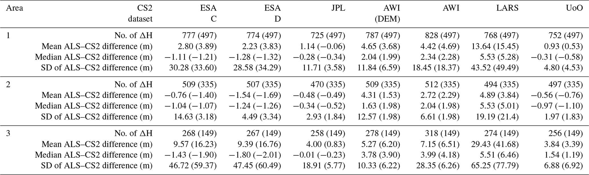
Figure 7 Left: the surface elevation measured by the CryoVEx airborne laser scanner (ALS). The thin black line outlines the entire study area (Area 1); the two subareas are indicated in the figure. Here, Area 3 is covering the complex surface topography of the surging basin of the Austfonna ice sheet. Right: the geolocations of the two ESA L2 baselines. Map data ©2019 Google.

3.3 Sea ice

3.3.1 Stack peakiness implementation

Statistics that describe the power of the CS2 waveform stack were already present in the previous baselines: stack kurtosis and stack standard deviation (SSD). While performing an explorative study focused on distinguishing leads from ice surfaces, the adoption of a further parameter was proposed: the stack peakiness (SP). This compares the maximum power registered in the range-integrated power (RIP) with the power obtained from the other looks. It is also important to notice that this is different from the peakiness of the multilooked waveform. The latter is influenced by all the looks (multilooked), while the SP compares the influence of the look with the highest power (supposedly at the nadir) with the looks taken at different viewing angles. The advantages in using the SP as a method of discriminating sea ice floes from leads, instead of (or together with) stack kurtosis (SK) and SSD, are described in Passaro et al. (2018). The temporal evolution of the SP over a sea-ice-covered area is compared with the SK and SSD stored in the official product (at the time of Baseline-C). The evolution of SP in the lead areas are similar: a peak, which corresponds to the strongest return from the zero-look angle compared to the other looks, is easily identifiable; the measurements close to the peak are characterized by a decay SP, which is still higher than the value found in the absence of a lead, since the latter can be the dominant return in the waveform up to about 1.5 km away from the subsatellite point (Armitage et al., 2014). The lead areas are also characterized by high kurtosis and low SSD, but these two indices fail to univocally show a local maximum or minimum. The kurtosis presents multiple peaks, which may be attributed to high power in nonzero look angles due to residual side-lobe effects; the SSD, being based on a Gaussian fitting, is not able to distinguish subtle differences in the power distribution of the very peaky RIP waveforms in the lead areas. The exact formula to compute SP and the thresholds are reported in Passaro et al. (2018). The SP has now been included in the new Baseline-D and is implemented in lead discrimination for L2 sea ice products (as discussed in Sect. 2.2).

3.3.2 CryoSat Baseline-D freeboard assessment

The different physical characteristics of sea ice and leads, which provide the local sea surface height, affect the shape and the power of the reflected radar pulses received by the altimeter, allowing for surface discrimination. Retracking echoes coming from sea ice and leads enables determination of the height of the sea ice and the sea level, respectively. Finally, the freeboard height is obtained by subtracting the local sea surface height from the sea ice elevations.

Previous analyses carried out by the Cryo-seaNice ESA project highlighted important overestimations in the freeboard values of the ESA CryoSat Baseline-C products relative to in situ data (see the recommendation Rec. 9 in CSEM Report, 2017). Following these conclusions, modifications have been made to develop the new ESA CryoSat Baseline-D freeboard product. We present here the first assessments of this updated version.

The freeboard maps in Fig. 8 present the differences between the two baselines. They demonstrate that the Baseline-D mean freeboard values have been significantly reduced. Aside from a mean bias of about 10 cm (see map Fig. 8c) the two solutions remain consistent with each other. The small patterns of higher differences (e.g., north of Greenland) are associated with statistically negligible noise at the ice margin zones. In addition, the root mean square (RMS) in each 20 km × 20 km pixel, referring to a small-scale freeboard variability, is similar for the two baselines (about 15 cm).

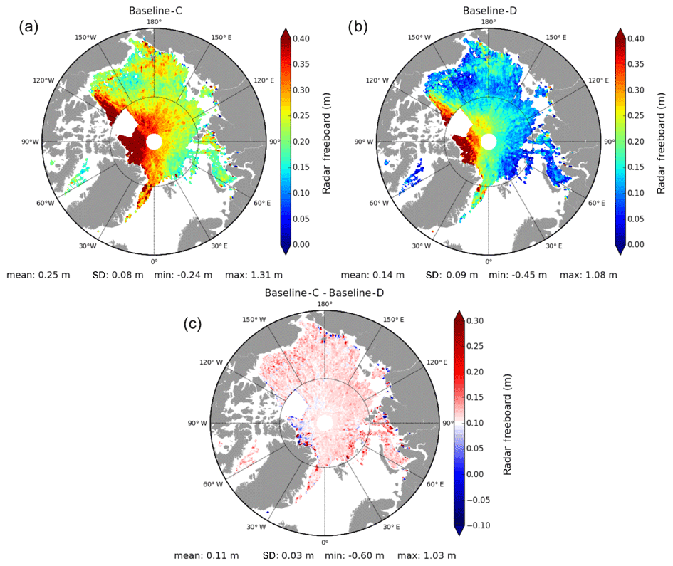
Figure 8 Monthly freeboard maps from 10 March to 11 April 2014 of the (a) Baseline-C and (b) Baseline-D versions. The third map (c) presents the difference between the two previous maps (Baseline-C–Baseline-D). Note that the map (c) color bar is centered on 0.1 m to underline the mean bias deviation between the two versions.

Figure 9 presents scatter comparisons with the Beaufort Gyre Exploration Project (BGEP; https://www.whoi.edu/beaufortgyre, last access: October 2019) and the National Snow and Ice Data Center (NSIDC) Operation IceBridge official product (OIB; https://daacdata.apps.nsidc.org/pub/DATASETS/ICEBRIDGE/Evaluation_Products/IceBridge_Sea_Ice_Freeboard_SnowDepth_and_Thickness_QuickLook, last access: October 2019) in situ measurements. To compute the OIB sea ice freeboard, we calculate the difference between the ATM (Airborne Topographic Mapper) mean total freeboard and the snow depth estimated from the snow radar. The freeboard radar is then deduced considering the decrease in radar velocity in the snow pack as follows:

$$\begin{array}{}\text{(1)}& {\displaystyle }& {\displaystyle }{\mathrm{FB}}_{\mathrm{ice}}={\mathrm{FB}}_{\mathrm{laser}}-\mathrm{snowdepth},\text{(2)}& {\displaystyle }& {\displaystyle }{\mathrm{FB}}_{\mathrm{radar}}={\mathrm{FB}}_{\mathrm{ice}}-\mathrm{snowdepth}\times {\left(\mathrm{1}+\mathrm{0},\mathrm{51}\times {\mathit{\rho }}_{\mathrm{s}}\right)}^{\left(-\mathrm{1.5}\right)},\end{array}$$

with ${\mathit{\rho }}_{\mathrm{s}}=\mathrm{0},\mathrm{3}$.

To compare with BGEP data, we compute a CryoSat Ice draft from the difference between the gridded sea ice thickness (that integrates the snow load) and ice freeboard data. Note that the ice freeboard is calculated from the radar freeboard taking into account the decrease in radar velocity in the snow pack using the formula specified in Eq. (2), with the snow depth provided by the Warren99 modified climatology (Warren et al., 1999) and the official OSI SAF (Ocean and Sea Ice Satellite Application Facility) sea-ice-type classification available at the NSIDC. To ensure the consistency between in situ measurements and altimetric observations, all data are projected onto monthly EASE2 500×500 grids identical to the one of the altimetric product. Each in situ measurement presented in Fig. 9 is the average of all data in a 12.5 km × 12.5 km grid pixel size. Relative to OIB, the Baseline-D freeboard mean bias is reduced by about 8 cm, which roughly corresponds to a 60 % decrease. The BGEP data indicate a similar tendency with a mean draft bias lowered from 0.85 to −0.14 m (mean draft is ∼ 1 to 1.5 m). For the two in situ datasets, the root mean square deviation (RMSD) is also well reduced from 14 to 11 cm for OIB and by a factor of 2 for the BGEP.

Figure 9 Illustration of the Baseline-D product improvements by comparison with in situ measurements. The first two panels compare the 2014 Operation IceBridge (OIB) freeboard measurements with (a) the Baseline-C and (b) the Baseline-D sea ice freeboard. The two following scatterplots compare the winter 2013/14 Beaufort Gyre Exploration Project (BGEP) sea ice freeboard converted to draft estimations with (c) the Baseline-C and (d) the Baseline-D sea ice freeboards.

Some additional comparisons have demonstrated that the Baseline-D freeboard solution is within the range values of recent freeboard estimations reported in Ricker et al. (2014) and Guerreiro et al. (2017). All together, these results demonstrate the positive improvements of the ESA Baseline-D freeboard product compared to the previous Baseline-C version. In addition, in sea-ice-covered regions, the accurate estimation of the sea surface height (SSH) highly depends on the number and spatial distribution of leads. A study by Armitage and Davidson (2014) showed that the CryoSat SARIn acquisition mode can be used to obtain a more precise SSH, as it enables processing of echoes that are usually discarded because of their ambiguity, e.g., echoes dominated by the reflection from off-nadir leads. In fact, the phase information available in the SARIn mode enables the across-track location on ground of the received echoes to be determined and an off-nadir range correction (ONC) to be geometrically computed, accounting for the range overestimation to off-nadir leads (Armitage et al., 2014). Thus, the ONC can correct for biases in the SSH retrieval due to off-nadir ranging, estimated to be 1–4 cm by Armitage et al. (2014). Additionally, the more precise SSH obtained from SARIn measurements can reduce by ∼ 29 % the average random uncertainty in freeboard estimates (Di Bella et al., 2018). Despite the overall reduction in the random freeboard uncertainty when including the phase information, pan-Arctic sea ice freeboard estimates from CryoSat Baseline-C SAR–SARIn L1B products showed large negative freeboard heights at the boundary of the SARIn mode mask (Fig. 10a and b). The analysis performed by Di Bella et al. (2019) attributed the negative freeboard pattern observed in Fig. 10a and b to large values of ONC, associated with inaccurate phase differences. The same study determined that the CAL4 correction, responsible for calibrating the phase difference between the signal received by the two antennas (Fornari et al., 2014), was not applied at the beginning of a SARIn acquisition.

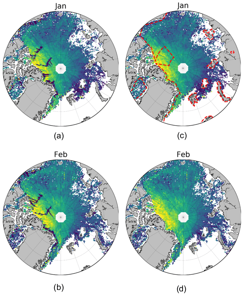
Figure 10 Gridded monthly freeboard from Baseline-C (a–b) and Baseline-D (c–d) L1b data for the period January–February 2014. The dashed red line in (c) represents the boundaries of the SARIn acquisition mask.

The Baseline-D SAR–SARIn IPF1 applies the CAL4 correction which is closest in time to the 19 bursts of the first SARIn acquisition, improving notably the phase difference and the coherence at the retracking point. Looking at the Arctic freeboard estimates obtained from Baseline-D SAR–SARIn L1B products in Fig. 10c and d, one can notice that the negative freeboard pattern along the boundaries of the SARIn acquisition mask has disappeared, highlighting a continuous freeboard spatial distribution throughout the Arctic Ocean.

The Baseline-D IPF1 therefore improves the quality of the retrieved heights in areas up to ∼ 12 km inside the SARIn acquisition mask, being beneficial not only for freeboard retrieval but also for any application that exploits the phase information from SARIn L1B products.

3.3.3 Impact of algorithm evolution on sea ice thickness consistency

Operational L1B products generated by the CryoSat Baseline-C Ice processor are a primary dataset for observing changes in sea ice thickness in the Northern Hemisphere. Examples of the application of CryoSat L1B products in sea ice climate research are formalized climate data records such as those of the ESA Climate Change Initiative (CCI; Paul et al., 2018; Hendricks et al., 2018b) and the Copernicus Climate Change Service (C3S; Hendricks et al., 2018a, b). In addition, several agencies and institutes generate sea ice data records based on the CryoSat L1B Baseline-C products (Tilling et al., 2018; Ricker et al., 2014; Kurtz et al., 2014; Kwok et al., 2015; Guerreiro et al., 2017). To estimate the impact of the algorithm evolution of the CryoSat Ice processor to Baseline-D on these sea ice data records, we compute sea ice thickness (SIT) for both Baseline-C and Baseline-D primary input datasets with an otherwise identical processing environment. The processing chain for this experiment has been developed at the Alfred Wegener Institute (AWI; Ricker et al., 2014), and we utilize the most recent algorithm version 2.1 (Hendricks et al., 2019). The AWI processor is implemented in the python sea ice radar altimetry library along with the climate data records of the ESA CCI and C3S. Processing steps consist of a L2 processor for the estimation of sea ice freeboard and thickness at full along-track resolution and a L2 processor for mapping data on a space–time grid for a monthly period with a resolution of 25 km in the Northern Hemisphere. For a full description of the algorithm and processing steps we direct the reader to Hendricks et al. (2019). The CryoSat Baseline-D input data are processed with an identical processor configuration to the current Baseline-C-based AWI reprocessed product line. The impact analysis is implemented for 5 months in the Baseline-D test period (October–November 2013, February–April 2014) by evaluating pointwise differences (Baseline-D–Baseline-C) in gridded thickness from the two CryoSat primary input versions. Monthly statistics of sea ice thickness differences (ΔSIT) itemized for all grid cells in the Northern Hemisphere (ALL) as well as for the SAR and SIN modes of the altimeter are shown in Fig. 11 and in Table 3.

Figure 11 (a) Time series of gridded monthly sea ice thickness difference (ΔSIT) statistics for the AWI sea ice processing chain based on the Baseline-D test dataset and Baseline-C input. Differences (Baseline-D minus Baseline-C) are color coded for all 25 km × 25 km grid cells in the Northern Hemisphere (ALL) and separately for SAR and SIN input data. The inner box indicates the median difference with the confidence interval; the square marker indicates mean difference ($\stackrel{\mathrm{‾}}{\mathrm{\Delta }\mathrm{SIT}}$) and the vertical line the maximum ΔSIT range. (b–d) SIT maps in April 2014 for Baseline-D (b), Baseline-C (d) and the Baseline-D–Baseline-C difference (c). The marked region WHB (Wingham Box) indicates an area where CryoSat operated in SIN mode.

Table 3 Mean thickness difference ($\stackrel{\mathrm{‾}}{\mathrm{\Delta }\mathrm{SIT}}$) and standard deviation (σ_ΔSIT) for all monthly gridded fields during the winter months (October–April) of the Baseline-D TDS. The statistics are broken down into (1) all grid cells with data coverage for both baselines (2) SAR data and (3) SIN data (highest ΔSIT values).

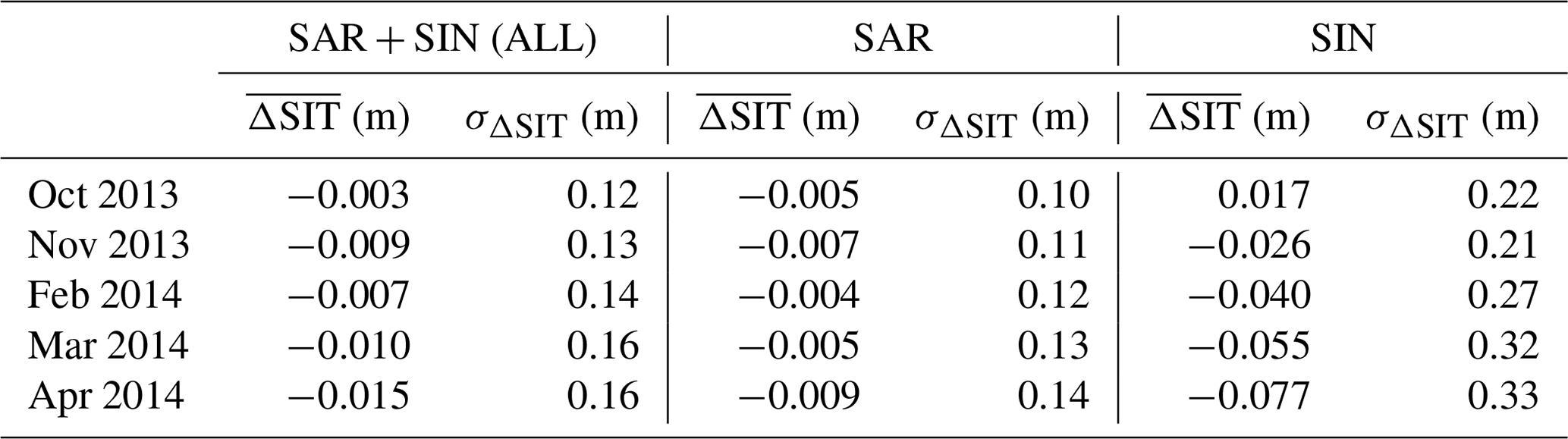
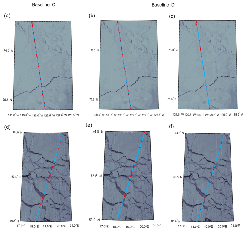
Figure 12 While red dots represent lead, light blue dots represent ice. (a–c) The MODIS images are from 17 October 2013, 22:10 UTC; CryoSat-2 passes over after 21 min. (d–f) The MODIS images are from 17 April 2014, 22:10 UTC; CryoSat-2 passes over after 5 min. The lead classification of Baseline-C based on Tilling et al. (2018) (a, d). The lead classification of Baseline-D based on Tilling et al. (2018) together with stack peakiness (b, c, e, f). (b, e) Leads are identified over stack peakiness over 13. (c, f) Leads are identified over stack peakiness over 15.

In addition, Fig. 11 illustrates the regional distribution of ΔSIT for the exemplary monthly period of April 2014. The mean monthly thickness difference between Baseline-D and Baseline-C ($\stackrel{\mathrm{‾}}{\mathrm{\Delta }\mathrm{SIT}}$) varies between −3 and −15 mm. Its magnitude increases over the winter season with its highest values in April, which we attribute to the increase in ice thicknesses over the winter period. However, the radar mode plays an important role in the $\stackrel{\mathrm{‾}}{\mathrm{\Delta }\mathrm{SIT}}$ result, as thickness measurements from SAR data are significantly less impacted by the input version than those from SIN data. Regions with SIN data therefore drive the magnitude and negative sign for hemispheric $\stackrel{\mathrm{‾}}{\mathrm{\Delta }\mathrm{SIT}}$ (SAR −5 to 9 mm; SIN −17 to −77 mm). On the map in Fig. 11 this is particularly visible in the Wingham Box (WHB), a region where CryoSat has operated in SIN mode from 2010 to 2014 and which has a higher density of grid cells with negative ΔSIT. The magnitude of ΔSIT even for SIN is however small compared to the SIT uncertainty for monthly gridded observations that are mostly driven by the unknown variability in snow depth, surface roughness and sea ice density. Average gridded SIT uncertainty in the AWI product for April 2014 is 0.64 m, and we therefore conclude that a maximum $\stackrel{\mathrm{‾}}{\mathrm{\Delta }\mathrm{SIT}}$ of −0.015 m in the period of the TDS is insignificant for the stability of sea ice data records. This bias also includes an issue in the Barents and Kara seas, where the number of orbits in the Baseline-D test dataset was less than in the Baseline-C data, and minor thickness differences can be observed in Fig. 11 due to this selection bias. This impact analysis however does not provide any insights into the specific algorithm changes that are causing the observed ΔSIT. We therefore speculate that the change in power scaling of L1B SIN waveforms, which was twice the expected waveform in Baseline-C and now corrected in Baseline-D, is the reason for the larger impact on SIN data as the AWI surface-type classification depends partly on total waveform backscatter. Specifically, we observed that fewer Baseline-D waveforms are classified as lead or sea ice (not shown) with a classification algorithm previously used for Baseline-C.

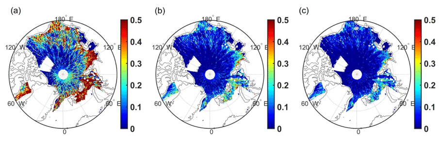
Figure 13 Monthly lead fraction maps based on Tilling et al. (2018) (a) and stack peakiness 13 (b) and 15 (c) in April 2011.

Figure 14 The percentage of good measurements for Baseline-C (blueish) and Baseline-D (coral) based on 26 tracks covering 15 Swedish lakes.

Therefore, the gridded thicknesses in both baselines in SIN mode areas are based on a different subset of input waveforms, which is far less the case in SAR mode areas. An update to the surface-type classification that includes the additional stack peakiness information in Baseline-D has the potential to further improve surface-type classification and consequently sea ice freeboard and thickness. The AWI processing chain is based on the python sea ice radar altimetry processing library (pysiral). The source code is available under a GNU General Public License v3.0 (https://github.com/shendric/pysiral, last access: June 2019). Reprocessed and operational sea ice thickness with intermediate parameters for gridded and trajectory products of the AWI processing chain can be accessed via the following FTP (ftp://ftp.awi.de/sea_ice/product/cryosat2/, last access: April 2019).

3.3.4 Lead classification comparison between CryoSat Baseline-C and Baseline-D

Lead classification is essential for retrieving sea ice freeboard and thickness. The stack peakiness (SP) introduced by Passaro et al. (2018) is included in Baseline-D. The SP, a new stack parameter, is known for helping isolate nadir returns. Passaro et al. (2018) show SP becomes higher when a lead approaches from off-nadir to nadir. The lead classification using SP identifies somewhat big and wide leads with SP over 13 and 15 (Fig. 12). SP 13 identified more leads than SP 15. Since features misclassified as leads attributed by off-nadir returns unseen in MODIS images are hard to quantify at the MODIS resolution scale, Passaro et al. (2018) confirm that the SP is able to avoid off-nadir lead return. The SP value should be optimized by evaluating the accuracy of ice freeboard and thickness. Adopting SP might consequently improve ice freeboard and thickness estimation by isolating nadir returns. A comparison in monthly lead fraction maps in April 2011 is shown in Fig. 13. The format of monthly lead fraction maps is the same as in Lee et al. (2018). As expected, while the spatial pattern of lead fraction is similar, overall lead fraction based on Tilling et al. (2018) is higher than lead fraction based on SP. Mean lead fraction in the whole Arctic based on Tilling et al. (2018), SP 13 and SP 15 is 0.14, 0.05 and 0.03, respectively. This difference likely affects ice freeboard and thickness estimation. This validation exercise shows that adopting SP might consequently improve ice freeboard and thickness estimation by isolating nadir returns.

3.4 Inland waters

While CryoSat was initially designed to measure the changes in the thickness of polar sea ice and the elevation of the ice sheets and mountain glaciers, the mission has gone above and beyond its original objectives. Scientists have discovered that CryoSat's altimeter has the capability to map sea level close to the coast and to profile land surfaces and inland-water targets such as small lakes, rivers and their intricate tributaries (Schneider et al., 2017). In this respect, to evaluate the new CryoSat Baseline-D TDS for lake level estimation, two study areas were selected: Sweden which is covered by SAR mode and the Tibetan Plateau which is covered by SARIn mode. Both areas have a dense concentration of lakes with a large range of sizes. In both cases the period September to November 2013 is studied. The evaluated products are the L2 products (SIR_SAR_L2 and SIR_SIN_L2) for Baseline-C and Baseline-D. The surface elevations are extracted using a water mask (Lehner and Döll, 2004, for Sweden and Jiang et al., 2017, for Tibetan Plateau) and referenced to the EGM2008 geoid model. In the evaluation the standard deviation of the individual water level measurements is estimated for each track and as a summary measure the median of the distribution of standard deviations (MSD) is used. Here we assume that the observations follow a mixture of Gaussian (70 %) and Cauchy (30 %) distributions. The mixture distribution is more robust and ensures that the estimated standard deviations are not too influenced by erroneous observations (Nielsen et al., 2015). Furthermore, the percentage of “good observations” is calculated. Here a good measurement is defined as a measurement within 1 m of the corresponding estimated track mean. The 1 m threshold is arbitrary and simply selected to establish a common reference. To obtain solid statistics only tracks with 15 or more measurements are used in the analysis. For comparison the analysis was conducted for both Baseline-C and Baseline-D. For the Swedish area the analysis is based on 26 tracks covering 15 lakes with areas ranging from 29 to 3559 km². It is found that the MSDs are 7.3 and 7.1 cm for Baseline-C and Baseline-D, respectively. With respect to the percentage of good observations, a convincing increase is observed for Baseline-D (Fig. 14). The larger number of valid measurements reduces the error in the mean lake level for each track, which is used in the construction of water level time series. On the Tibetan Plateau, 104 tracks covering 57 lakes with areas between 101 and 2407 km² are investigated. It is found that the MSDs are 19.2 and 18.8 cm for Baseline-C and Baseline-D, respectively. Furthermore, the approximately 60 m offset in the surface elevation that is present in Baseline-C is eliminated in Baseline-D. For Baseline-D a slight increase in the percentage of good observations, generally around 5 %–10 % for most lakes, is observed.

4 Conclusions

In conclusion, validation activities presented in this paper confirm that the new Baseline-D Ice L1B and L2 data show significant improvements with respect to Baseline-C over land ice, sea ice and inland-water domains, while the migration to netCDF makes these new products more user-friendly than the previous EEF products. The assessment of a 6-month TDS by multithematic CryoSat expert users was instrumental in confirming data quality and providing an endorsement from the scientific community before the transfer of the Baseline-D Ice processors to operational production on 27 May 2019. The Baseline-D algorithms show significant improvements over all kinds of surfaces. Most notably, freeboard is less noisy, is no longer overestimated and scatter comparisons with in situ measurements confirm the improvements of the Baseline-D freeboard product quality with a reduction in mean bias by about 8 cm, which roughly corresponds to a 60 % decrease with respect to Baseline-C. For the two in situ datasets considered (OIB and BGEP) the RMSD is also well reduced from 14 to 11 cm for OIB and by a factor of 2 for the BGEP. In addition, freeboard no longer shows discontinuities at SAR–SARIn interfaces. Over land ice, the main improvements are due to the increased accuracy in the roll angle. This has provided better results with respect to the previous baseline when comparing the data to a reference DEM over the Austfonna ice cap region and improved the ascending and descending crossover mean from 1.9 to 0.1 m. Inland-water users also reported significant improvements including a reduction in previously observed measurement outliers and an increased percentage of good observations, generally around 5 %–10 % for most lakes. Overall, this new CryoSat processing Baseline-D will maximize the uptake and use of CryoSat data by scientific users since it offers improved capability for monitoring the complex and multiscale changes in the thickness of sea ice, the elevation of ice sheets and mountain glaciers, and their effect on climate change.