the Creative Commons Attribution 4.0 License.
the Creative Commons Attribution 4.0 License.
 | 09 Jun 2020
The RHOSSA campaign: multi-resolution monitoring of the seasonal evolution of the structure and mechanical stability of an alpine snowpack
Bettina Richter
Henning Löwe
Cecilia Cetti
Judith ter Schure
Alec Van Herwijnen
Charles Fierz
Matthias Jaggi
Martin Schneebeli
The necessity of characterizing snow through objective, physically motivated parameters has led to new model formulations and new measurement techniques. Consequently, essential structural parameters such as density and specific surface area (for basic characterization) or mechanical parameters such as the critical crack length (for avalanche stability characterization) gradually replace the semiempirical indices acquired from traditional stratigraphy. These advances come along with new demands and potentials for validation. To this end, we conducted the RHOSSA field campaign, in reference to density (ρ) and specific surface area (SSA), at the Weissfluhjoch research site in the Swiss Alps to provide a multi-instrument, multi-resolution dataset of density, SSA and critical crack length over the complete winter season of 2015–2016. In this paper, we present the design of the campaign and a basic analysis of the measurements alongside predictions from the model SNOWPACK. To bridge between traditional and new methods, the campaign comprises traditional profiles, density cutter, IceCube, SnowMicroPen (SMP), micro-computed-tomography, propagation saw tests and compression tests. To bridge between different temporal resolutions, the traditional weekly to biweekly (every 2 weeks, used in this sense throughout the paper) snow pits were complemented by daily SMP measurements. From the latter, we derived a recalibration of the statistical retrieval of density and SSA for SMP version 4 that yields an unprecedented spatiotemporal picture of the seasonal evolution of density and SSA in a snowpack. Finally, we provide an intercomparison of measured and modeled estimates of density and SSA for four characteristic layers over the entire season to demonstrate the potential of high-temporal-resolution monitoring for snowpack model validation.
- Article
(10024 KB) - Full-text XML
- BibTeX
- EndNote


Regular snow monitoring programs are one of the cornerstones of snow science providing valuable time series of snow properties (e.g., Reba et al., 2011; Morin et al., 2012; Landry et al., 2014; Wayand et al., 2015; Leppänen et al., 2016; Lejeune et al., 2019). Such time series are indispensable for the development and evaluation of snow models (e.g., Fierz, 1998; Etchevers et al., 2004; Morin et al., 2013; Essery et al., 2016; Krinner et al., 2018) as well as for various applications such as snowpack stability assessment for avalanche risk forecasting (e.g., Schweizer and Wiesinger, 2001; van Herwijnen and Jamieson, 2007), snowpack processes studies (e.g., Dumont et al., 2017), snow property retrievals from remote sensing (e.g., Leinss et al., 2016; King et al., 2018), water resource estimations (e.g., Jonas et al., 2009), climate studies (e.g., Takala et al., 2011) or instrument developments (e.g., Schneebeli et al., 1998). Worldwide many study sites have been established for snow monitoring (Ménard et al., 2019). Col de Porte in France (Lejeune et al., 2019), Sodankylä in Finland (Leppänen et al., 2016) and Weissfluhjoch (WFJ) in Switzerland (Meister, 2009) offer some of the longest time series of snowpack observations, dating back to 1936 in the case of WFJ. Regular snowpack monitoring programs rely on weekly to biweekly manual observations and measurements, by digging snow pits along a profile line in the (nearly) homogeneous observation area. Observations comprise mainly traditional profiling with a characterization of layer properties (grain size, grain shape, hand hardness and wetness) and measurements of ram resistance and snow temperatures, all following standard procedures (Fierz et al., 2009). Those measurements are typically complemented by so-called snow stability test, such as the compression test (Jamieson, 1999; van Herwijnen and Jamieson, 2007), to monitor weak layers and snow mechanical properties in view of avalanche forecasting. Although these traditional characterization methods are well-established, they suffer from well-known problems of quantitative objectivity, limiting their use for physical snow modeling.
To address this issue, efforts have shown a clear tendency of replacing traditional measurements with newly developed field methods to obtain more objectively defined snow properties. Concerning the characterization of snow microstructure, the observer-biased estimate of traditional grain size can be replaced by measurements of specific surface area (SSA) (Morin et al., 2013; Leppänen et al., 2015). It is defined by the ice–air interface surface area divided by the snow mass, which is inversely proportional to the optical grain size. SSA drives many snow processes such as metamorphism, radiation interaction, air flow and chemical reactions and thus plays an important role in many large-scale processes such as surface energy balance (e.g., Domine et al., 2007). Different field instruments were developed to measure SSA based on similar methods such as DUFISSS (Gallet et al., 2009), POSSSUM (Arnaud et al., 2011), IRIS (Montpetit et al., 2012) or IceCube (Zuanon, 2013). Concerning snowpack stability assessment, classical stability tests are now often complemented by the propagation saw test (PST), developed about a decade ago to objectively characterize the crack propagation propensity based on the critical crack length parameter (Gauthier and Jamieson, 2006; Sigrist and Schweizer, 2007; van Herwijnen and Jamieson, 2005). The critical crack length corresponds to the length of a saw cut manually introduced in a buried weak layer leading to rapid crack propagation (e.g., Gauthier and Jamieson, 2008). Additional mechanical parameters can be obtained when combining PSTs with particle tracking velocimetry (van Herwijnen et al., 2016).
These latest advances in field measurements coincide with similar improvements in detailed snowpack models such as Crocus (Brun et al., 1992; Vionnet et al., 2012) and SNOWPACK (Lehning et al., 2002b; Wever et al., 2015). The modeling of SSA as a prognostic variable was included in Crocus to replace the empirical grain size parameter (Carmagnola et al., 2014) and indirectly estimated in SNOWPACK from the grain size, dendricity and sphericity (Vionnet et al., 2012). Modeling the SSA allows for an unambiguous comparison with SSA measurements. In addition, many snow properties can now be formulated using physical principles that naturally involve the SSA as a parameter. Likewise, a new model of the critical cut length based on objective stratigraphic information was implemented in SNOWPACK (Gaume et al., 2017) and recently refined to support avalanche risk forecasting (Richter et al., 2019).
These advances, coherently developed in field techniques and modeling, come along with new demands for validation campaigns. If snow models are only validated against surface or bulk measurements instead of the full stratigraphy, the compensation of effects may prevent the detection of model errors (e.g., Essery et al., 2013; Lafaysse et al., 2017). However, only a few quantitative evaluations of density and SSA profiles exist (Morin et al., 2013; Leppänen et al., 2015; Wever et al., 2015; Essery et al., 2016). Presently, the evaluation of density and SSA is partly limited by the temporal and spatial resolution of measured profiles, which are typically conducted on a weekly to biweekly basis with a vertical resolution of 3 cm or set by the layers. In contrast, modeled profiles can be provided hourly and at sub-centimeter vertical resolutions. The gap in resolutions between measurements and models precludes the evaluation of snow processes occurring on short timescales and/or locally in the snowpack, such as surface hoar formation (e.g., Stössel et al., 2010), faceting (e.g., Pinzer et al., 2012) or crust formation. Concerning the critical cut length, Richter et al. (2019) reported a good agreement between the temporal evolution of the critical crack length measured in the field and modeled from the refined parameterization. They also highlighted the capability of the parameterization to detect weak layers in simulated snow profiles.
Increasing the spatiotemporal resolution of measurements is still cumbersome due to inherent time constraints for snow pits and manual measurements. Towards a remedy, recent studies utilized the micro-penetrometer SnowMicroPen (SMP) (Schneebeli et al., 1999) for both microstructure characterization and stability assessment. Proksch et al. (2015) presented a statistical method to retrieve density and SSA from SMP data, and Reuter et al. (2015) suggested an approach to estimate point snow instability from SMP data. These examples exploit key advantages of the SMP, namely fast profiling for frequent measurements and high vertical resolution, so that profiles are obtained at a considerably finer scale (mm) than possible with traditional means. Though principally promising, the use of the SMP within snow monitoring programs has never been assessed and would require a comprehensive comparison to other methods to evaluate uncertainties.
In the context raised above, the value of emergent, objective snow properties, their potential to replace traditional means in operational snow monitoring programs and their requirements at temporal and vertical resolutions for model evaluations can be investigated within a multi-resolution and multi-instrument dataset to facilitate comprehensive cross-comparison analyses. We strive to provide such a resource in the form of the outcome of an extensive snow measurement campaign which is referred to as RHOSSA in resemblance of the Greek letter ρ for density and SSA. The campaign was carried out at the WFJ site from December 2015 to March 2016 and comprises
-
daily full-depth profiles of density and SSA of 0.5 mm vertical resolution derived from SMP measurements;
-
weekly full-depth profiles of density and SSA of 3 cm vertical resolution from manual snow pit measurements;
-
biweekly full-depth traditional profiles with layer-dependent vertical resolution, completed with PST and classical stability tests;
-
occasional profiles of the 3D microstructure at 18 µm vertical resolution from X-ray tomography (not full depth, only on selected heights in the snowpack, mostly focusing on defined layers of interest).
Our main results comprise (1) new, recalibrated parameterizations to derive density and SSA from SMP 4 measurements; (2) the evolution of density and SSA profiles at unprecedented spatial and temporal resolution; (3) the evolution of snow instability from various stability tests; (4) a comparison of the density and SSA estimates over time for distinct layers of the snowpack; and (5) a comparison between measured values of density and SSA and modeled ones from standard SNOWPACK runs that documents the state of the art and highlights the potential of high-resolution stratigraphy data for snow model evaluation and future developments.
The paper is organized as follows. Section 2 provides an overview of the design of the RHOSSA campaign. Sections 3 and 4 describe the measurement methods and the simulations with SNOWPACK, respectively. Section 5 presents specific data analysis methods applied to exploit the RHOSSA dataset, namely a redefined statistical model for density and SSA retrievals from SMP 4 measurements and a layer tracking method to monitor the evolution of specific layers of the snowpack over the season. Section 6 provides a first analysis of the RHOSSA dataset in terms of stratigraphy, stability, density and SSA, including cross comparisons between measurements and the evaluation of SNOWPACK simulations. Specific points are finally discussed in Sect. 7.
During the winter of 2015–2016, the snow observation program at the WFJ site, located in the eastern Swiss Alps above Davos (elevation of 2536 m, latitude 46.82963∘ N, longitude 9.80925∘ E), was supplemented with additional measurements, forming all together the RHOSSA field campaign. We focused on the period from the beginning of December 2015 to the end of March 2016 to ensure measurements in dry snow conditions as required by some of the used instruments. In addition, measurements were done in the morning typically starting at 08:00 GTM+2. The RHOSSA campaign included traditional profiling, stability tests, density cutter measurements, IceCube measurements, SMP measurements and tomography. Using such a wide range of measurement methods resulted in different temporal resolutions (frequency) and spatial resolutions (vertical along the snow profile), as synthesized in Table 1. SMP measurements were performed daily, density cutter measurements and IceCube measurements were performed once a week, and traditional snow profiles were recorded on a weekly to biweekly basis and completed with stability tests. X-ray tomography measurements of extracted, decimeter-sized samples were occasionally performed six times during the season at selected locations to image some defined layers of interest and allow further comparisons. Spatial resolutions range from 0.1 mm for the tomography-based properties to the size of the snow layer for the traditional profiling (typically from 1 to 30 cm).
The measurement field at the WFJ site is a flat area of about 20 m×8 m (Fig. 1). To ensure an efficient use of the snow field, measurements were performed within defined areas. The snow field was divided into three corridors, each 20 m long and 1.5 m wide, as illustrated in Fig. 1. Throughout the season, sets of measurements were performed, moving continuously along the corridor in daily steps, starting at one end of corridor 1 and ending at the end of corridor 3, with two consecutive sets of measurements being at least 30 cm apart to avoid disturbances. A schematic of the location of three consecutive sets of measurements (“day 1”, “day 2” and “day 3”) performed in corridor 2 at mid-season is shown in Fig. 1. Each corridor was divided lengthwise in two parts of 75 cm wide. One side was reserved for stability tests (red area in Fig. 1); the other side was used for all the other measurements. First, the five daily SMP measurements with a 15 cm spacing were performed perpendicular to the corridor direction (black dots in Fig. 1). Then, during a snow pit day as illustrated by “day 2” in Fig. 1, the pit was dug such that the pit wall was parallel and a few centimeters behind the line that was formed by the SMP measurements. Density cutter and IceCube measurements were done next to each other (blue and orange areas in Fig. 1) and complemented by a traditional snow profile when needed (green area in Fig. 1). Finally, for the occasional X-ray tomography, undisturbed snow blocks were extracted from the pit wall near the location of the other measurements.
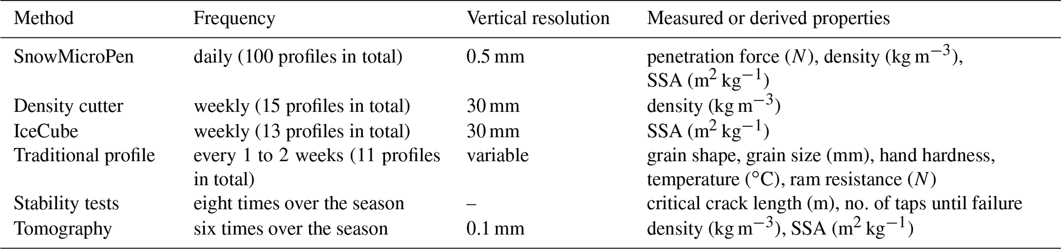
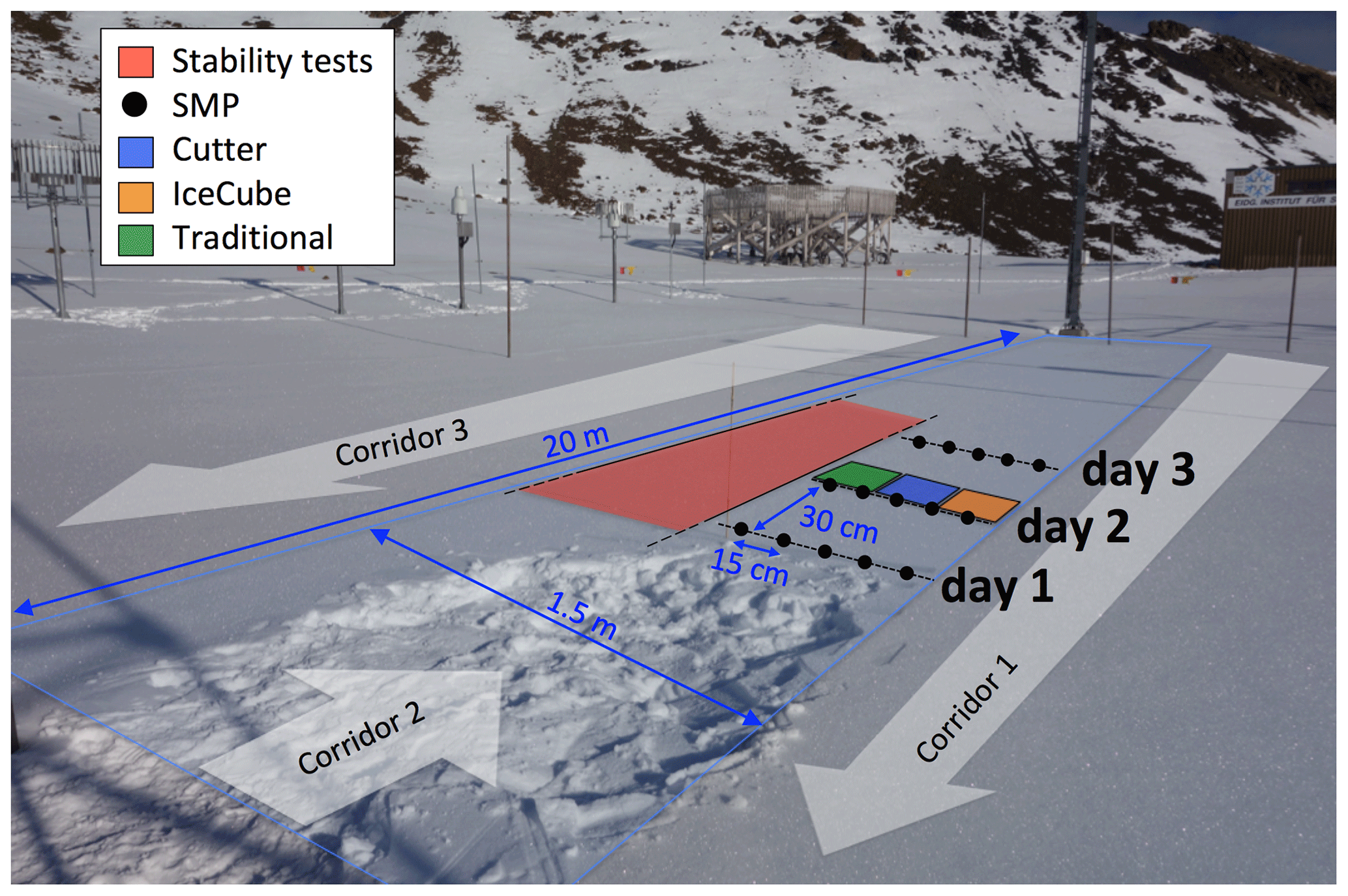
Figure 1 Picture of the snow field where measurements of the RHOSSA campaign were performed. The location of each measurement is illustrated for 3 consecutive days.
3.1 Traditional profile and stability tests
Traditional snow profiles were observed to characterize snow stratigraphy by hand hardness, grain size and grain type. In addition, ram resistance, snow temperatures and water equivalent of the snow cover were measured (Fierz et al., 2009). Snow stability tests were performed to identify potential weak layers and evaluate the load required for failure. Specifically, we performed the compression test (CT; van Herwijnen and Jamieson, 2007), the extended column test (ECT; Simenhois and Birkeland, 2009) and the propagation saw test (PST; Gauthier and Jamieson, 2008). In a CT or an ECT, the snowpack is progressively loaded by tapping on a snow shovel placed on the snow surface with increasing force (10 taps from the wrist, 10 taps from the elbow and 10 taps from the shoulder). If a failure occurs within the snow cover, the loading step, i.e., the number of taps at which the failure occurred, is recorded. In a CT, which consists of an isolated column of 30 cm by 30 cm, information describing the type of failure is also recorded (for more details see van Herwijnen and Jamieson, 2007). In an ECT, which consists of an isolated column of 30 cm by 90 cm, the propagation distance across the column is recorded as no propagation, partial propagation or full propagation (for more details see Simenhois and Birkeland, 2009). CT and ECT are thus used to identify potential weak layers and qualify the loading required for failure. The PST, on the other hand, is used to measure the critical crack length required for crack propagation in an a priori known weak layer. It consists of an isolated 30 cm wide column with a length of at least 120 cm, which has been excavated to below the weak layer of interest. An artificial crack is then created by drawing a snow saw through the weak layer until the critical crack length is reached and rapid crack propagation occurs. The critical crack length is recorded as well as the propagation distance, where END refers to cracks which propagated to the end of the column (for more details see Gauthier and Jamieson, 2008).
3.2 Density cutter
A density cutter was used to manually record the density profile of the snowpack by performing successive measurements from the surface to the bottom of the snowpack with a vertical resolution of 3 cm. A box-type density cutter of 100 cm3 (3 cm × 5.5 cm × 6 cm) (Carroll, 1977; Conger and McClung, 2009; Proksch et al., 2016) was used to measure density by weighing a snow sample extracted from the cutter. A measurement error of about 10 % can be expected (Carroll, 1977; Conger and McClung, 2009; Proksch et al., 2016), with the typical source of errors being the measurement of compacted snow volumes (overestimation) when extracting light snow and of incomplete snow volumes (underestimation) when extracting fragile snow (e.g., faceted crystals or depth hoar).
3.3 IceCube
The IceCube was used to measure an SSA profile of the snowpack by performing successive IceCube measurements from the surface to the bottom with a vertical resolution of 3 cm. The IceCube is an optical system commercialized by A2 Photonic Sensors (Zuanon, 2013) to retrieve SSA from measurements of the infrared hemispherical reflectance of snow (Gallet et al., 2009). Briefly, a snow sample is illuminated with a 1310 nm light diode and the light reflected by the snow surface is recorded. The signal is recorded as voltage values and then converted into reflectance values based on a voltage-to-reflectance calibration curve obtained using certified optic standards. SSA values are finally estimated from the reflectance values using the parametrization of Gallet et al. (2009). The complete description of the measurement principle can be found in Gallet et al. (2009). Measurements were performed on cylindrical snow samples with a 6 cm diameter and 2.5 cm height, extracted from the snow pit following the method given by Gallet et al. (2009) and Zuanon (2013). Snow samples were very slightly compressed when inserted into the sample holder and attention was paid to have a flat snow sample surface. Measurement uncertainty was estimated to about 10 % for SSA values below 60 m2 kg−1, as for the DUFISSS device. Additional measurement artifacts occur for snow with higher SSA that can lead to over-estimated SSA values (Gallet et al., 2009).
3.4 SnowMicroPen
The SnowMicroPen (SMP), a digital cone penetrometer, was used to measure the vertical penetration resistance profile of the snowpack. From that, density and SSA profiles were derived based on a statistical model and after a specific signal processing, as described in Sect. 5.1. The SMP consists of a motorized probe that is driven vertically into the snowpack at a constant speed of 20 mm s−1 to measure the penetration resistance exerted on a cone (diameter of 5 cm and cone half angle of 30∘) located at the tip of the probe (Schneebeli et al., 1999). We used a version 4 SMP with a 2 m rod and recorded penetration resistance with a vertical resolution of 1/242 mm. Two preliminary measurements were systematically performed to cool the SMP towards snow temperature before the five daily measurements were taken. The quality control of SMP force profiles was done manually by rejecting signals with (1) visible trends either in the air portion of the signal or over the entire depth, (2) high noise levels and unrealistic spikes, and (3) frozen tip problems revealed by a force response that appears to be activated only deeper in the snowpack. Most of these problems are caused by wet conditions. The air–snow and snow–ground interface were detected manually to remove air and ground regions from the signal.
3.5 Micro-computed tomography
X-ray micro-computed tomography was used to image the 3D microstructure of snow samples extracted from the snowpack at selected locations. Snow blocks of about 30 cm × 30 cm × 30 cm were cut out from the profile wall on 14 December, 13 January, 27 January, 10 February, 16 February and 2 March. The location of the extracted blocks within the snowpack were chosen subjectively, either to ensure temporal continuity with a previously sampled block or to refocus on a particular layer of interest, mainly persistent weak layers. Extracted blocks were sealed in Styrofoam boxes and filled with dry ice (about −80 ∘C) for transportation from the field site to the cold lab (duration approximately 1 h). In the lab, the blocks were stored at −25 ∘C and successively subsampled into sample holders of 7 cm height and 3.6 cm diameter. These samples were then scanned in a cooled micro-computer tomograph (μCT 80, Scanco Medical) with a resolution of 18 µm voxel size. The reconstruction utilized standard procedures with noise reduction by Gaussian filtering (support=2 voxels; width=1.2 voxels) and binary segmentation following the method of Hagenmuller et al. (2013). From the binary 3D images, density and SSA were computed over a moving window of 120 pixel height obtaining profiles at a vertical resolution of about 2 mm.

Figure 2(a) Density from cutter measurements against density derived from SMP data using the parametrization of Proksch et al. (2015) (blue circles) and the recalibrated present parametrization (red circles). (b) SSA from IceCube measurements against SSA derived from SMP data using both parametrizations.
To put the measurement campaign in context, we conducted standard simulations with the detailed snow cover model SNOWPACK (Wever et al., 2015; Lehning et al., 2002b) using version 3.4.1, revision 1473 (https://models.slf.ch/p/snowpack/, last access: 5 June 2020). The snowpack itself is considered to be a linear viscoelastic material, the settlement of which was calculated as described in Sect. 2.2.2 in Lehning et al. (2002b) and taking into account the impact of load rate. This new scheme also implies an altered viscosity parameterization (both unpublished). Liquid water flow in snow was solved using the Richards equation recently implemented by Wever et al. (2014). Neumann boundary conditions were used at the snow–atmosphere boundary, whereas a constant geothermal heat flux of 0.06 W m−2 was applied at the bottom of the 3 m deep soil column. A total of 32 layers with thickness increasing from 1 to 40 cm with depth make up this column. A late summer iso-thermal temperature profile of 5 ∘C was assumed. The simulation was initiated on 1 September 2015 with no snow on the ground until 14 October 2015 except for 1.5 d in September (snow height less than 11 cm). This results in a spin-up time of 43 d before the WFJ site was snowed in.
The model was driven with an optimized half-hourly dataset of meteorological and snowpack measurements from the automatic weather station at the WFJ site (WSL Institute for Snow and Avalanche Research SLF, 2015). The dataset is well-described in Wever et al. (2015) and contains standard meteorological measurements including air temperature (ventilated), relative humidity (ventilated), wind speed, shortwave and longwave radiation (both fluxes each), and undercatch corrected precipitation. The set also includes automatically measured snow height that was used to drive the snow cover accumulation, that is, by the increments of measured snow height. The added mass is then obtained from the density of new snow computed using an empirical relation between air temperature and wind speed (Schmucki et al., 2014). To account for rainfall, we used the precipitation data whenever the air temperature exceeded 1.2 ∘C (see Schmucki et al., 2014). Snow albedo was forced from the in situ measurements of incoming and reflected shortwave radiation fluxes. The calculated values underwent a plausibility check and in the case of a negative outcome were replaced by the model parametrization (less than 0.8 % of the values). The surface sensible and latent heat flux parameterizations are derived from Monin–Obukhov similarity (Lehning et al., 2002a).
The time step for the simulation was set to 15 min and output was written every 60 min. For this campaign, we were particularly interested in evaluating the model in terms of density and SSA. The latter was simply retrieved from the optical diameter of snow that is empirically derived from dendricity, sphericity and grain size according to Vionnet et al. (2012).
5.1 Deriving density and SSA from SMP
As a prerequisite to derive density and SSA from SMP measurements, it was necessary to modify the current statistical models of Proksch et al. (2015). When applying the parametrizations of Proksch et al. (2015), SMP-derived density and SSA compared rather poorly to values from cutter and IceCube measurements, respectively (Fig. 2). This is in part due to the fact that the parametrizations of Proksch et al. (2015) were derived from measurements with an SMP device version 2 whereas we used a newer SMP version 4 that contains different electronic components leading to different force correlations at a small scale. We thus derived a recalibration of the statistical models of Proksch et al. (2015) to better match our snow pit measurements. The obtained density and SSA parametrizations are called new parameterizations hereafter.
The idea of Proksch et al. (2015) was to relate a dataset of some relevant SMP micro-parameters to a reference dataset of density (or SSA) from tomographic images using a statistical multi-linear regression model, all datasets being obtained from independent, co-located and co-temporal measurements. The SMP micro-parameters consist of the median of the penetration resistance force and a characteristic length of the microstructure L (akin to the distance between two ruptures), as defined in the stochastic model of Löwe and van Herwijnen (2012). Here we followed the same procedure but took our cutter measurements as reference data of density (ρcutter) and our IceCube measurements as reference data of SSA (SSAic), instead of tomographic data. The statistical modeling was applied based on a sub-dataset of data from the days for which both SMP and snow pit measurements were available (15 d for density, 13 d for SSA). From each raw force signals, parameters and L were computed from the raw penetration force profiles over a sliding window of 1 mm with 50 % overlap, yielding profiles of and L with a vertical resolution of 0.5 mm. Note that Proksch et al. (2015) used a sliding window of 2.5 mm, but tests with different window heights (1, 2.5 and 5 mm) did not show a significant impact. Next, for each day, the five daily profiles of and L of the same day were aligned by simply using snow surface as a common reference, and a median operation was applied to get one representative profile of and L per day, called the median profiles in the following. Next, each median profile was averaged vertically using a 3 cm window to match the vertical resolution of the snow pit measurements. Finally, the median 3 cm averaged profiles of and L and the profiles of ρcutter and SSAic of the same day were aligned by using snow surface again as the common reference and cropped to the length of the shortest profile. This way, all profiles of a given day are described on the same vertical scale and values of , L, ρcutter and SSAic can be paired for the statistical modeling, relying on a total of 590 paired values for density and 497 for SSA.
Based on this sub-dataset, we applied a regression of the form
to estimate density from and L by least-squares optimization (ρcutter being the target). The following parameters were obtained: , , and , where ρsmp is in kilograms per cubic meter, L in millimeters and in newtons, and where the errors denote the standard errors of the regression. This regression has a R2 coefficient of 0.79, a residual standard error of 40.8 kg m−3 and p values less than 10−3. Differing slightly from the one suggested by Proksch et al. (2015), a regression of the form
was applied to estimate SSA by least-squares optimization (SSAic being the target). The following regression parameters were obtained: , and , where SSAsmp is in square meters per kilogram. This regression has a R2 coefficient of 0.67, a residual standard error of 8.4 m2 kg−1 and p values less than 10−3.
The performance of the new parametrizations compared to the original parametrizations of Proksch et al. (2015) is presented in Fig. 2. This plot shows the observed density from cutter measurements compared with the SMP-derived density obtained from Eq. (1) and from Proksch et al. (2015) for the 15 d for which both data are available (same dataset as used for the statistical modeling). Similarly, the observed SSAs from IceCube measurements are presented against the SMP-derived SSA from Eq. (2) and from Proksch et al. (2015) for the 13 d for which both data were available (same dataset as used for the statistical modeling). To do so, and as done for the statistical modeling, SMP-derived properties were averaged over 3 cm resolution, and SMP and snow pit profiles of the same day were realigned with the snow surface and cropped to the length of the shortest profile. As expected, SMP-derived properties are closer to the snow pit measurements when using the present parametrizations. Applying a simple linear correlation between ρcutter and ρsmp, a R2 coefficient of 0.87 and a root-mean-square deviation (RMSD) of 34 kg m−3 are found when using Eq. (1) against a R2 of 0.75 and a RMSD of 69 kg m−3 when using the parametrization of Proksch et al. (2015). Between SSAic and SSAsmp, a R2 coefficient of 0.82 and a RMSD of 7 m2 kg−1 are found when using Eq. (2) against a R2 of 0.65 and a RMSD of 14 m2 kg−1 when using the parametrization of Proksch et al. (2015). In the following, the present parametrizations in Eqs. (1) and (2) were applied to all the SMP data, so that a daily density profile and a daily SSA profile at 0.5 mm vertical resolution were retrieved from the daily median signal of and L.
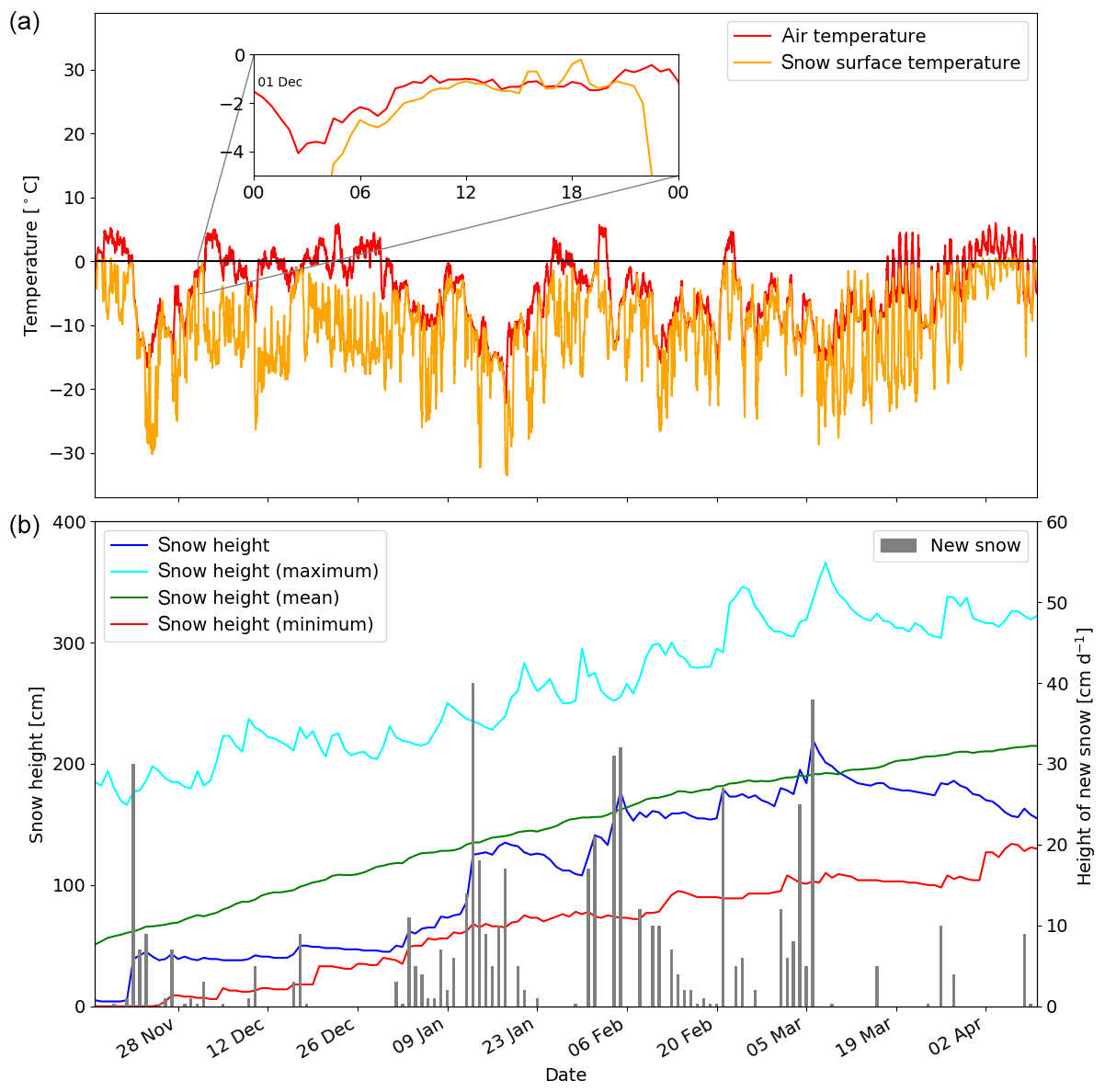
Figure 3 (a) Evolution of air temperature (red) and snow surface temperature (orange) at the WFJ site during winter 2015–2016. The inset shows data recorded on 1 December 2015 when the MF layer formed. (b) Seasonal evolution of snow height (blue) and height of new snow (gray bars). For context, the 80-year daily maximum (cyan), minimum (red) and mean (green) snow heights are also shown.
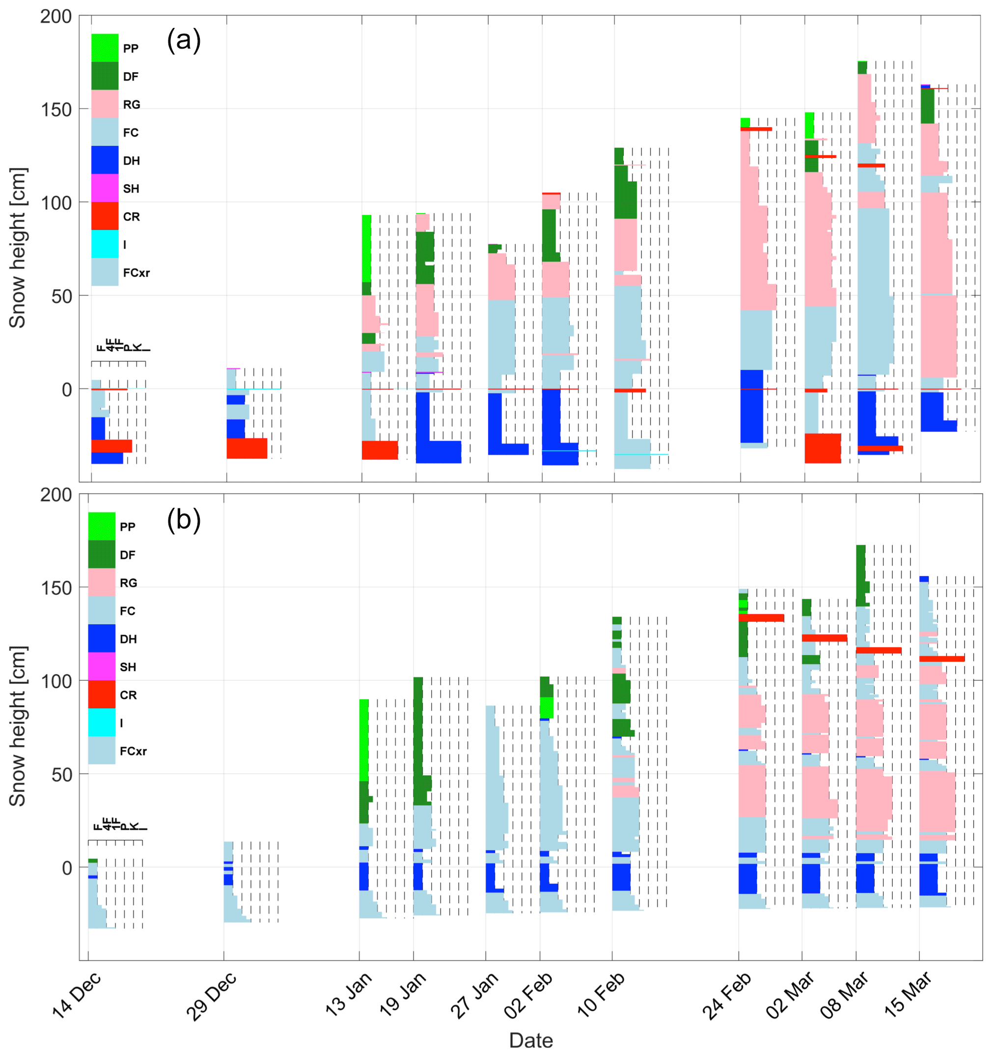
Figure 4 (a) Manual snow profiles observed during the 2015–2016 winter season. The colors indicate the major grain shape (red: melt forms, light blue: faceted crystals; blue: depth hoar; pink: rounded grains; green: decomposing and fragmented particles; light green: precipitation particles) and the width indicates the hand hardness. Snow height is relative to the top of the MF layer. (b) Simulated snow profiles for the same dates.
5.2 Layer tracking
We present a method to track particular layers of the snowpack throughout the season and retrieve their properties. This method will allow us to evaluate the measurement methods and simulation results later by comparing them in selected layers.
The first step is to define which are the layers of interest, knowing that this method is only possible with layers that contrast well enough with their surroundings so their boundaries can be easily identified by a rather sharp transition in the vertical profile of snow properties. In this study, we chose to track four directly adjacent layers located in the bottom part of the snowpack called the DH (depth hoar) layer, the MF (melt form) layer, the FC (faceted crystal) layer and the RG (rounded grain) layer, from bottom to top, referring to the predominant grain shape observed in the layer. They are described in detail in the next section. We chose these layers because they are among the main stratigraphic features of the snowpack observed during the winter, showed a wide range of snow types and properties, could be tracked over the entire winter, and were relatively easy to identify (rather sharp property transitions).
In the measurement data, the four layers of interest were defined by the height of their upper and lower boundaries. Boundaries were manually identified by simply looking at the property profiles, looking for sharp and relevant transitions, and recording heights. This step was performed on all the weekly density profiles from the cutter and SSA profiles from IceCube, as well as on all the daily representative profiles of penetration force resistance obtained from the five daily SMP measurements. The identification of layer boundaries was sometimes challenging for weak stratigraphic transitions, e.g., the transition between a layer of fresh snow and the soft snow layer it fell on. To help in such cases, boundaries could be backtracked in time, starting from a profile where the layer of interest is older and its boundaries more clearly detectable. Also, additional information, such as observed height of new snow, was sometimes used to help delineate boundaries. Based on the referenced boundaries, bulk properties of the layers of interest were computed for each date by averaging data within the recorded heights.
To identify the layers of interest in the SNOWPACK simulations, we used their date of deposition, which is one of the standard layer parameters simulated by SNOWPACK. To do so, we attributed a time stamp (YYMMDD) to each of the defined layer boundaries that corresponds to the date of deposition of the adjacent layer above it. Time stamps were determined using automatic weather station data as well as daily manual observations of the snow surface. A layer of interest was then simply defined as all the simulated layers with a deposition date older than the time stamp of its lower boundary and younger than the time stamp of its upper boundary. This way, the four layers tracked in this study were identified based on four boundaries called 151201-boundary, 151202-boundary, 160102-boundary and 160117-boundary, from the lower to the upper boundaries, and the ground. The DH layer was located between the ground and the 151201-boundary, MF layer between the 151201-boundary and the 151202-boundary, FC layer between the 151202-boundary and the 160102-boundary, and RG layer between the 160102-boundary and the 160117-boundary.

Figure 5 Stability test results for the DH layer (blue) and FC layer (red). The number of hits for CT (circles) and ECT (diamonds) and the critical crack length obtained from the PST (crosses) are shown. Black symbols indicate that the CT or the ECT did not result in a failure in the layers.
This section presents a basic analysis of the RHOSSA campaign alongside measurement intercomparisons and a preliminary evaluation of the SNOWPACK simulations. To present the evolution of profile properties with time, profiles presented in the following were realigned such that z=0 cm corresponds to the height of the upper boundary of the MF layer (i.e., the 20151202-boundary). Choosing this layer as a height reference leads to a better visual match than by simply taking the ground as reference (the field site ground at WFJ being uneven).
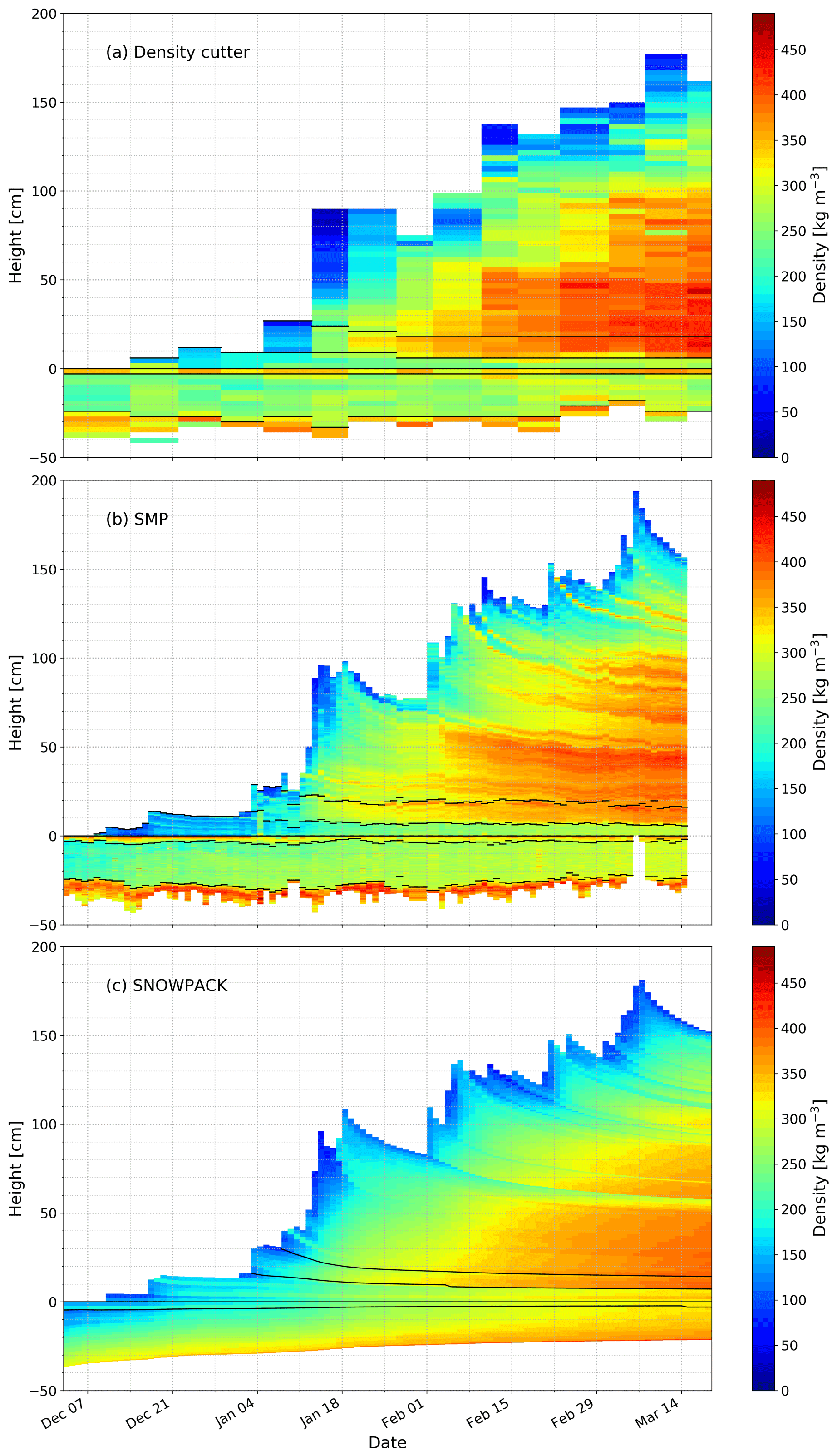
Figure 6 Evolution of the density profile during winter 2015–2016 (a) from cutter measurements, (b) derived from SMP measurements and (c) simulated by SNOWPACK. Boundaries shown with black lines allow identification of the four tracked layers (DF layer, MF layer, FC layer and RG layer, from bottom to top). Measurements below the lowest boundary shown in SMP, and cutter data were not considered part of the DF layer.
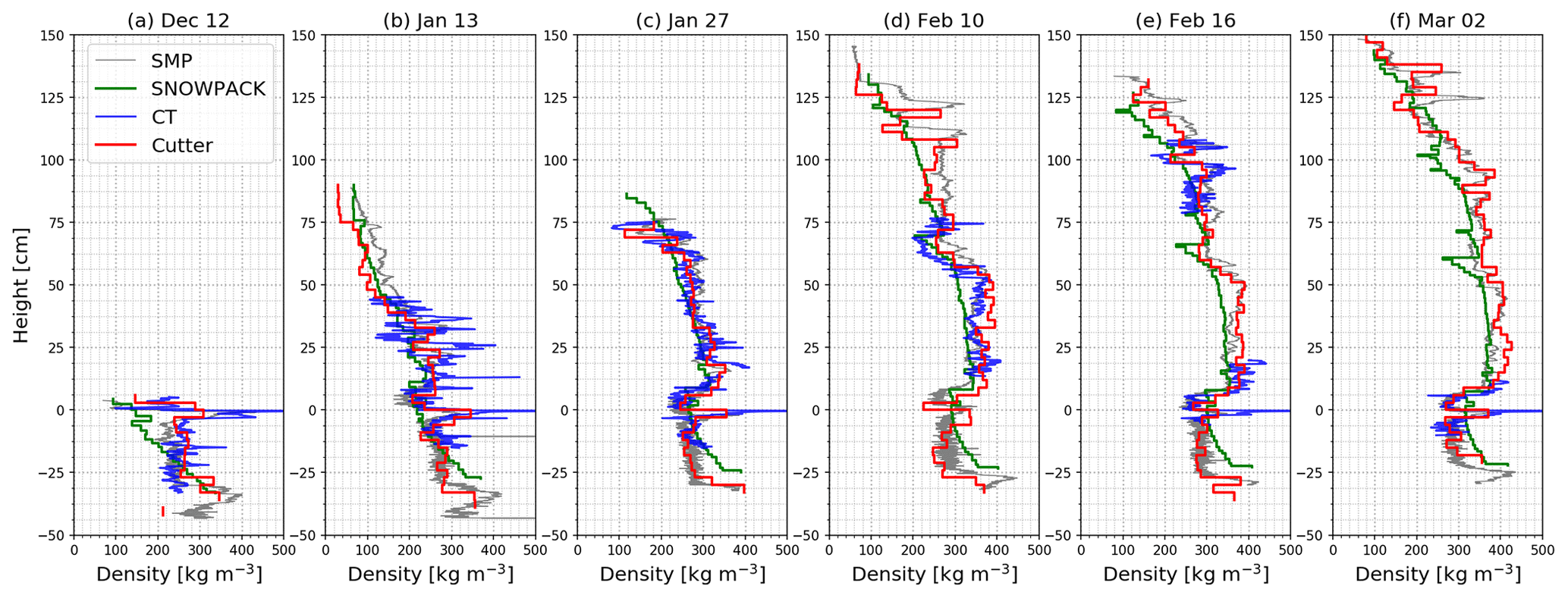
Figure 7 Vertical profiles of density from tomography, IceCube and SMP measurements as well as modeled by SNOWPACK.
6.1 Evolution of weather, snow stratigraphy and stability
To provide background information for the origin of stratigraphic features of the season, Fig. 3 shows the seasonal evolution of air and snow surface temperature as well as total snow height and height of new snow over 24 h. The biweekly traditional profiles observed between 14 December 2015 and 15 March 2016 are presented in the upper panel of Fig. 4. We can first note that winter 2015–2016 showed a below-average snow height, especially at the beginning of the season (Fig. 3). At the end of November, the winter started with a precipitation event after which the snow height reached approximately 40 cm. Thereafter, a dry period followed during which snow surface temperature remained between −20 and −10 ∘C, allowing large temperature gradients to build up across the shallow snowpack. Traditional profiles show that this basal layer recrystallized predominantly into depth hoar (dark blue layers below 0 cm in Fig. 4, upper panel), although faceted crystals and melt forms were sometimes also reported (light blue and red layers) and persisted throughout the season. This basal layer corresponds to the tracked layer referred to as the DH layer (Sect. 5.2). In the late afternoon of 1 December 2015, observers from the nearby ski resort reported rainfall up to 2600 m, and measured snow surface temperature reached 0 ∘C while the air temperature remained colder (see inset in Fig. 3), indicating freezing rain. This rainfall event led to the formation of a melt–freeze crust and rain crust at the snow surface, as reported in the traditional profile that followed on 14 December (Fig. 4, red and turquoise layer at 0 cm). This crust was persistent throughout the season and tracked as the MF layer. Mid-December, about 10 cm of new snow accumulated on this crust and recrystallized into faceted crystals by the end of December, favored by a period of rather clear weather leading to low snow surface temperatures (Fig. 3). Again, this layer of faceted crystals was observed throughout the season (light blue layers between about 0 cm and 10 cm in Fig. 4, upper) and corresponds to the tracked FC layer. January was generally characterized by more cloudy weather with consistent precipitation events (Fig. 3). With the first snowfalls early January, snow accumulated on top of the FC layer and was quickly buried by the subsequent heavy precipitation events, being buried under around 75 cm of snow by mid-January. This layer was protected from significant temperature gradients and evolved into small faceted crystals and rounded grains (light blue and light red layers between about 10 and 25 cm in Fig. 4). As this layer systematically showed a higher hand hardness (four fingers against one finger) and a smaller grain size (not shown) than the FC layer and DH layer, this layer was named the RG layer for the sake of differentiation. Finally, after further precipitation events mostly occurring in early February and early March, the snowpack height reached about 200 cm by mid-March and consisted mostly of layers of rounded grains on a weaker base of facets and depth hoar.
The snowpack stratigraphy simulated by SNOWPACK is shown in the lower panel of Fig. 4. Qualitatively, modeled stratigraphy compared well with observed stratigraphy. Indeed, although many subtle differences in grain shape and hand hardness exist throughout the season, the major stratigraphic features are well-reproduced, notably the weak base layers (DH layer and FC layer) as well as the overlying slab which mostly consisted of small rounded or faceted grains for which the hardness increases from top to bottom. Note also the lower density of the base layer compared to the overlying slab. One major discrepancy is that the melt–freeze and rain crust which formed on 1 December (MF layer) was not simulated by SNOWPACK (see dedicated comment in Sect. 7.3). Instead, SNOWPACK simulated around 3 cm of new snow, which later recrystallized into faceted crystals.
Snow stability tests showed that the weak base, namely the DH layer and FC layer, was the most critical weak layer during most of the season. As shown in Fig. 5, both layers consistently failed in CT and ETC until the beginning of February. Thereafter, these layers were not reactive anymore as tapping on the snow surface was not affecting the weak base buried below the hard and thick slab (black symbols in Fig. 5). From the PST, it was possible to follow the evolution of the critical crack length throughout the season (crosses in Fig. 5). Overall, the critical crack length increased steadily from about 20 cm in mid-January to around 60 cm in the beginning of March for both the FC layer and DH layer, indicating weak layers less and less prone to crack propagation with time. Note that the critical crack length was consistently lower for the DH layer than for the FC layer.
6.2 Evolution of density
Figure 6 presents the evolution of the density profile during winter, as recorded from density cutter measurements, derived from SMP measurements, and simulated by SNOWPACK. Boundaries of the tracked layers are identified with solid black lines. The snowpack evolution is characterized by the punctual presence of new snow at the surface, showing the lowest density values down to about 50 kg m−3. Overall, snow gets gradually denser upon deeper burial in the snowpack and as the season progresses, reaching density values as high as 450 kg m−3 in the middle of the snowpack by midwinter. Despite being located in the bottom of the snowpack, the persistent weak layers (DH layer and FC layer) remain significantly lighter than the adjacent layers. Finally, density of the MF layer remains roughly constant throughout the winter at around 350 kg m−3.
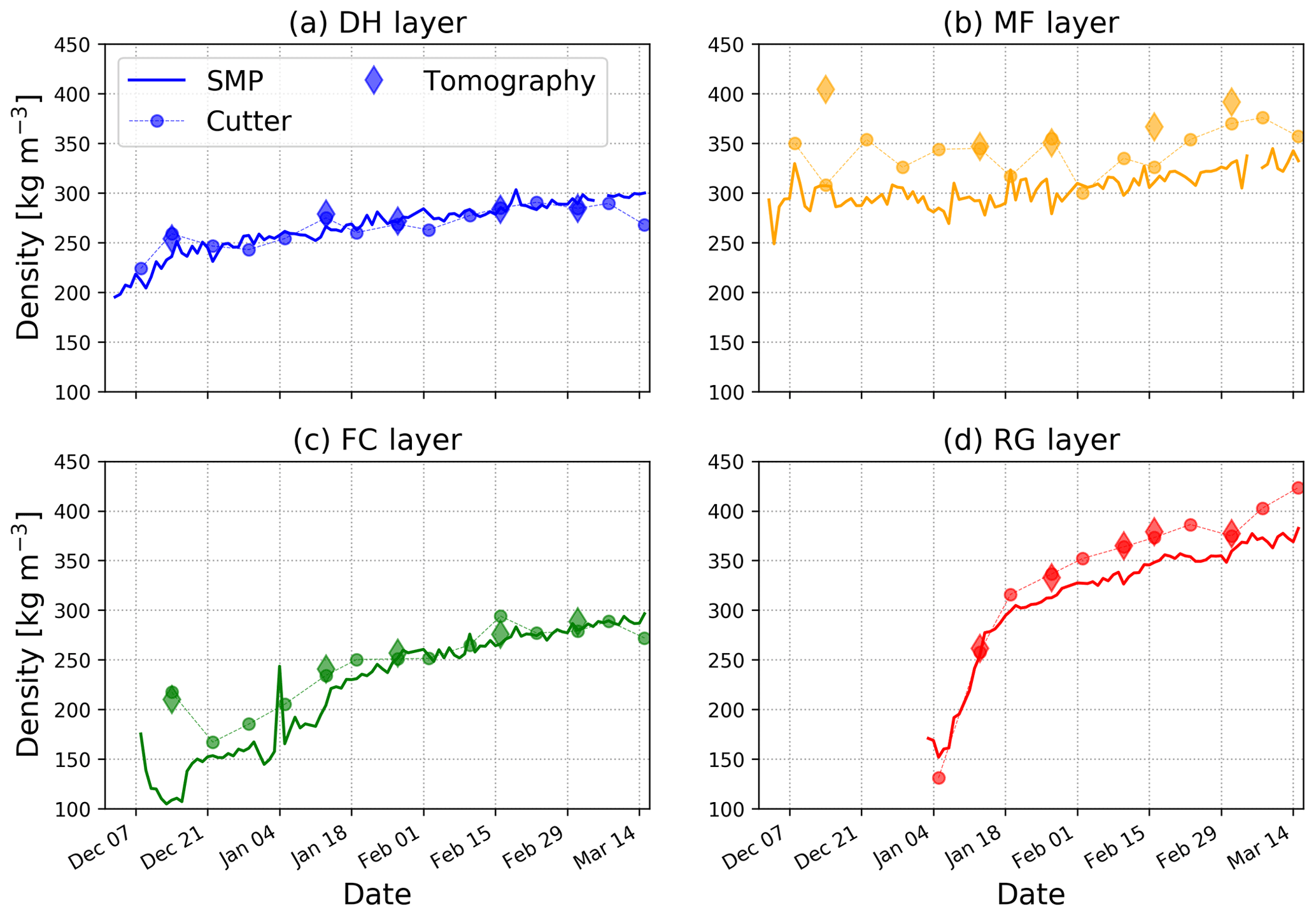
Figure 8 Density evolution of the four tracked layers from SMP, density cutter and tomography measurements as well as modeled by SNOWPACK.
Although these features are consistently reported by both measurement methods, many stratigraphic details are only revealed by the SMP measurements and are not captured by the cutter measurements. The high temporal and spatial resolution of the SMP measurements allows us to almost continuously follow the evolution of density with time. For instance, we can clearly follow the density evolution of the 2 cm thick snow layer from its formation on 22 February showing density values around 350 kg m−3 (layer located at 145 cm height on 22 February in Fig. 6b) to mid-March when buried under about 40 cm of snow but still showing similar density values (layer located at 115 cm height on 15 March in Fig. 6b). The evolution of this layer is not or only diffusely captured by the cutter measurements. Note that this layer was reported in the traditional profiles from 24 February on as a layer of melt forms with a hand harness of one fist (Fig. 4).
The next figures allow comparison of tomography, cutter and SMP measurement, as well as simulations from SNOWPACK, in greater detail. Figure 7 shows the vertical profiles of density for 6 d of the season. Figure 8 shows the evolution of density for the four tracked layers, DH layer, MF layer, FC layer and RG layer, throughout the winter. Both figures highlight an overall consistency between measurements. A slightly larger scatter is observed in the density evolution of the MF layer (Fig. 8b), which might be partly due to uncertainties in the definition of the layer boundary (see Sect. 7.1). One can also note the decrease in density recorded by the last two cutter measurements for the DH layer and FC layer (Fig. 8a and c). This might reflect a measurement bias that can occur when sampling fragile snow layers (under-sampling).
Simulations of the density profiles over the season agree overall well with the observations (Fig. 6c). The mis-modeling of the MF layer, as mentioned earlier, leads however to large local deviations. Moreover, SNOWPACK seems to overestimate the densification rate of the DH layer and FC layer, leading to significantly higher modeled values by mid-March (Fig. 8a and c). This overestimation can also be observed in the vertical profiles for both weak layers for example (Fig. 7b–f). Inversely, densification rate seems to be underestimated for layers evolving from fresh snow to rounded grains in the upper part of the snowpack, leading to simulated densities lower than the measured ones by mid-March, as shown in Figs. 6 and 7f (layers from about 20 to 100 cm height). Finally, other inconsistencies can be observed locally in the simulated stratigraphy, such as the two relatively denser layers observed near the surface on 2 March at around 125 and 135 cm (Fig. 7b).
6.3 Evolution of SSA
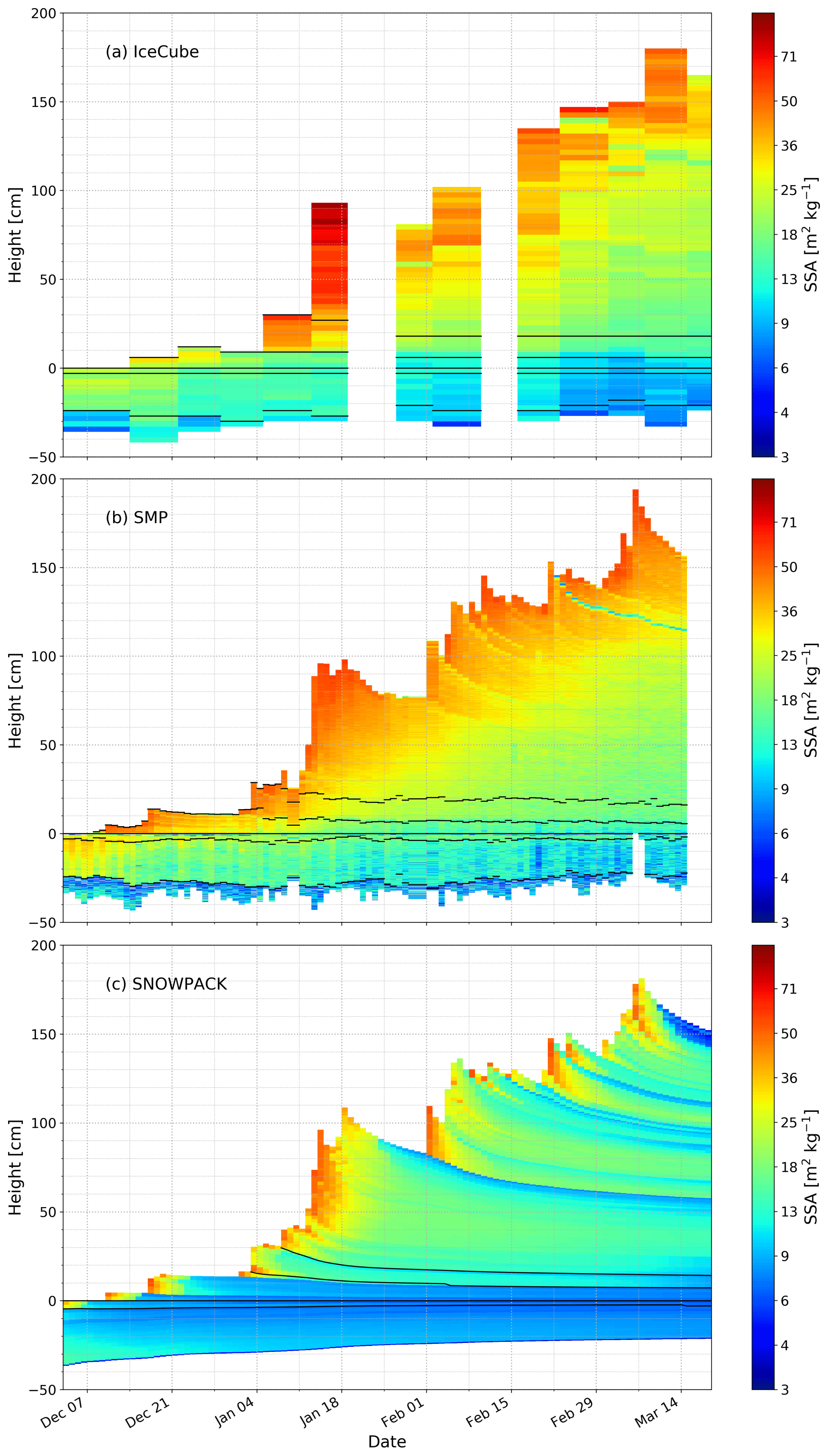
Figure 9 shows the evolution of the SSA profiles over the course of the winter from IceCube measurements from SMP measurements, and from SNOWPACK simulations. Note that IceCube measurements could not be performed on 19 January and 10 February 2016. SSA values range from about 70 m2 kg−1, for fresh snow layers at the surface, to about 5 m2 kg−1, in the bottom part of the snowpack. The MF layer, identifiable in terms of density (Fig. 6a and b), is here difficult to distinguish from the DH layer and the FC layer due to their similar SSA values. The general trend of the SSA evolution is an overall decrease with time and depth. The impact of the spatial and temporal resolution is again highlighted. For instance, the evolution of the layer deposited on 22 February, easily identified by lower SSA values (greenish colors) than the ones of the adjacent layers, is clearly captured by the SMP measurements but only diffusely reported in the IceCube data.
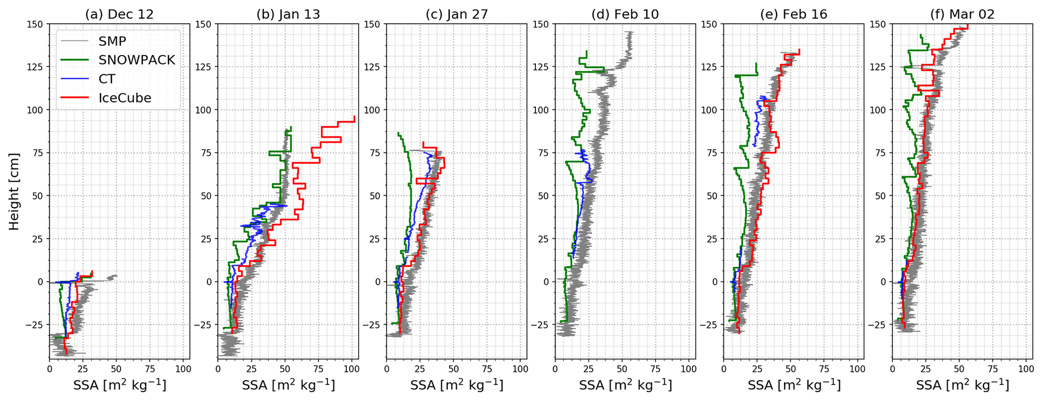
Figure 10 Vertical profiles of SSA from tomography, IceCube and SMP measurements as well as modeled by SNOWPACK.
To compare further, the vertical profiles of SSA for 6 d of the winter are shown in Fig. 10, and the temporal evolution of the SSA of the four distinct layers (DH layer, MF layer, FC layer and RG layer) is presented in Fig. 11. In particular, the latter figure allows analysis of the SSA decrease with time. The RG layer shows the largest decrease, especially shortly after deposition when SSA evolves from about 45 to 20 m2 kg−1 within 1 week. The SSA decay in the MF layer and the DH layer is slower, decreasing from about 15 to 10 m2 kg−1 within the whole course of the season.
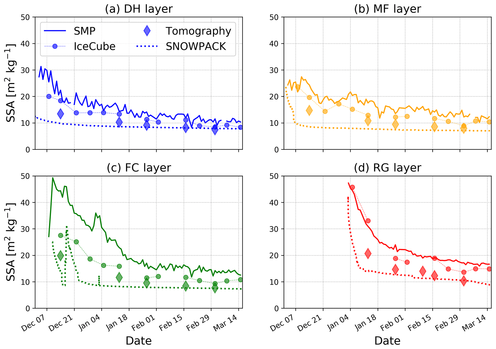
Figure 11 SSA evolution of the four tracked layers from SMP, IceCube and tomography measurements as well as modeled by SNOWPACK.
Both figures highlight significant disagreements between measurement methods. Looking at the vertical profiles (Fig. 10), SSA values from IceCube measurements are systematically higher than values from tomography measurements, by a factor of about 1.3. Besides this systematic bias, large deviations are found on 13 January 2016 in the upper half of the snowpack, for which SSA values from IceCube measurements range from 60 and 100 m2 kg−1, whereas values from SMP measurements do not exceed 50 m2 kg−1 (Fig. 10b, upper 60 cm). Possible causes for these deviations are discussed in Sect. 7.3.
Finally, SNOWPACK overall underestimates SSA compared to measurements (Figs. 9, 10 and 11). Deviations are higher with the IceCube data than the tomographic data, for which some good agreements can locally be found, for instance when looking at the SSA evolution of the tracked layers from mid-January on (excluding the MF layer).
7.1 The RHOSSA dataset for snow model evaluation
The presented dataset can be utilized as validation data for the evaluation of snow model outputs for the case of a dry alpine snowpack and over one winter season. Output parameters that can be evaluated are density, SSA, critical cut length, traditional snow pit measurements (grain size, grain type, hardness, temperature) and results from compression and extended compression tests. Snow models can be driven using the optimized forcing dataset, which includes meteorological and snow data from automatic and manual observations, provided in this study (Sect. 4). The RHOSSA dataset alone does not allow for robust and complete model evaluations, as model performances can vary depending on years and sites (Essery et al., 2013; Krinner et al., 2018). Yet, the snowpack monitored over winter 2015–2016 offered a wide range of alpine snow type and property variations throughout the season. It included typical persistent weak layers at the bottom of the snowpack (DH layer and FC layer) relevant for stability assessment for avalanche risk forecasting. Although the study focused on dry snowpack, some rain/melt events are also represented by the presence of several melt–refreeze crusts.
The specificity of the RHOSSA dataset is to provide time series of density and SSA at a daily frequency and with a vertical resolution of 0.5 mm, in contrast with previous validation datasets (weekly to biweekly, vertical resolution of 3 cm or higher) (e.g., Morin et al., 2013; Leppänen et al., 2015). Both temporal and spatial resolution are critical to account for in snow models because thin layers as well as processes occurring within short timescales can have a significant impact on the snowpack behavior, e.g., on its mechanical stability (e.g Jamieson and Johnston, 1992). We highlight the need of high-resolution datasets, as provided here, to evaluate the simulation of such features and processes.
In addition to validation datasets, comparison methods are also crucial when assessing models. Different methods were presented in the past to compare measurements and simulations: (i) the comparison of averaged (bulk) values over the entire snowpack height (e.g., Landry et al., 2014; Leppänen et al., 2015; Essery et al., 2016), which is easy to implement but provides rather limited information; (ii) the comparison of paired values at the same height of the snowpack, which allows assessment of the snowpack stratigraphy (e.g., Lehning et al., 2001; Morin et al., 2013) (as in Figs. 7 and 10); and (iii) the comparison of values averaged within boundaries of specific layers of the snowpack, as used in Wever et al. (2015) and in this study (Figs. 8 and 11). This latter method seems particularly suitable to assess the skill of parameterizations of internal snow processes, e.g., temporal evolution of density and SSA of a fresh snow layer or of a buried layer of surface hoar. Layer property evolution is indeed very close to the formulation of equations in a Lagrangian model. Methods (ii) and (iii) bear with uncertainties from vertical mismatches that might contribute to the scatter between measurements and simulations and should thus be first corrected. When comparing paired values at the same height, the prior alignment of the profiles is necessary. In the present case, we could simply realign the profiles thanks to the presence of the dominant MF layer in all measurement methods and throughout the season. Slight vertical mismatches can however be found. For example, the density profile of 2 March 2016 (Fig. 7) shows two distinct denser layers at around 125 and 135 cm height which are well-identified in both SMP and density cutter measurements but with a height mismatch of about 5 cm. This realignment method based on the identification of a persistent and well-defined snowpack feature might however not be always applicable. A more systematic approach could be the algorithm presented by Hagenmuller and Pilloix (2016) to automatically match snow profiles by adjusting their layer thicknesses. This method has a strong potential for quantitative comparison studies (Hagenmuller et al., 2018). When comparing properties of specific layers, the definition of the layer boundaries is critical. The fluctuations observed in the evolution of density and SSA of the MF layer (Figs. 8 and 11), especially visible in the SMP data, might possibly result from the boundary definitions of this layer, in addition to the natural spatial variability of snow. Besides, the manual definition of boundaries is rather time-consuming if numerous layers are tracked. A more automatic method could be developed. In this respect, the RHOSSA data constitute a valuable resource due to the continuity of the spatiotemporal picture of the seasonal evolution of stratigraphy.
7.2 The potential of daily SMP measurements
With daily SMP measurements, the RHOSSA campaign allows us to follow the evolution of the internal structure of a snowpack at a sub-centimeter vertical resolution almost continuously over 4 months – up to now inaccessible. An unparalleled smooth picture of the spatiotemporal evolution of density and SSA is revealed, contrasting with data from the classical snow pit measurements (Figs. 6 and 9). Many thin stratigraphic features are indeed clearly visible in the SMP data but only diffusely shown by the manual measurements. This highly detailed picture of the snowpack evolution opens new opportunities for field studies on snowpack processes occurring over short timescales (e.g., densification of fresh snow) or very localized (e.g., rain crust or surface hoar formation) as well as refined evaluation of snow models as already mentioned.
One advantage of SMP measurements compared to snow pit measurements is they are relatively faster (of the order of 30 min for five measurements) and thus more suitable for daily snowpack monitoring. It is however important to keep in mind that density and SSA are not directly measured by the SMP but derived from the force signal based on parameterizations (Fig. 2), bearing additional uncertainties comparing to other more direct measurements. Several parametrizations were previously put forward to derive density and/or SSA from SMP signals (e.g., Pielmeier and Schneebeli, 2003; Dadic et al., 2008; Proksch et al., 2015; Kaur and Satyawali, 2017). Differences between the parameterizations of density and SSA of Proksch et al. (2015) and the ones presented in this study are due to the version of the SMP device which has undergone an update of the electronics in version 4 that affected the inversion of the model from Löwe and van Herwijnen (2012) through the force correlation function. We would hope that the parameterizations of Eqs. (1) and (2) are generally applicable to SMP version 4. However, without an independent validation by measurements under different snowpack conditions, it is not possible to state the range of validity of the parametrizations presented here. In the long term, it would be desirable to improve the underlying stochastic–mechanical approach (Löwe and van Herwijnen, 2012) by an invertible model that contains density and SSA to retrieve these parameters from a more physical picture of the penetration process.
7.3 Comparing density and SSA estimates
As possible starting points to future dedicated studies, we sum up here the main deviations reported in this paper when comparing density and SSA estimates. First, we recall that density and SSA derived from SMP data were obtained to best match results from the cutter and IceCube measurements, so they necessarily inherit their performances.
We report a significant and systematic inter-measurement deviation in the SSA estimates. Values from IceCube and SMP are systematically higher than values computed on tomographic images, approximately by a factor of 1.3 (Fig. 10). A comprehensive comparison between optical methods, such as IceCube, and tomography seems very much needed to understand this systematic deviation. Besides, large disagreements were reported on the specific day of 13 January 2016, for which IceCube data range from 60 to 100 m2 kg−1 whereas SMP data show values around 50 m2 kg−1 (Fig. 10b). That day, measurements were performed during a snowfall in light freshly deposited snow. When measuring SSA of light snow, typically for values above 60 m2 kg−1, the emitted radiations can interact with the bottom of the sample holder during the measurement, causing an overestimation of the SSA (Gallet et al., 2009; Zuanon, 2013). Another possible cause is that the present statistical model used to derive SSA from SMP measurements fails to reproduce the high SSA values of newly deposited snow because of their underrepresentations (1 d) in the IceCube dataset used for calibration (similarly but to a lower extent, disagreements are found in the upper 20 cm of the density profiles of the same day (Fig. 7a): SMP measurements fail to capture the very low density measured by the cutter method (60 kg m−3 vs. 30 kg m−3)). Note that one major discrepancy between IceCube and SMP-derived SSA can be directly linked to the SSA calibration Eq. (2) that leads largely to overestimate the SSA values below about 20 m2 kg−1 by the SMP compared to IceCube (see Fig. 2b; data cloud is mostly located below the 1:1 curve). This can be clearly seen in our results (Figs. 9, 10 and 11) as a large part of the snowpack shows SSA values below 20 m2 kg−1.
Comparing SNOWPACK outputs against observations, one significant deviation is the absence of the MF layer in the simulations. This is due to the fact that the precipitation forcing scheme used in the present simulations does not allow the representation of rainfall events occurring at negative air temperatures. This inappropriate forcing could be improved by using diagnostic atmospheric variables to detect such events Quéno et al. (2018). Also, SNOWPACK underestimates SSA overall (Figs. 9, 10 and 11). A similar bias was reported at an arctic site (Leppänen et al., 2015). On the contrary, a systematic overestimation of the SSA simulated by Crocus was recently pointed out (Tuzet et al., 2017). Evaluations can however be challenged by the significant inter-measurement deviations observed, as discussed above. The agreement between simulations and estimates from tomography is better than between simulations and estimates from SMP or IceCube. Finally, recent publications point to contradicting performance of SNOWPACK to simulate the properties of depth hoar layers. While some studies report rather poor performance in matching observed density in Arctic environments (Domine et al., 2019; Gouttevin et al., 2018), others showed that SNOWPACK captures the density of basal layers in Alpine snowpacks fairly well (Wever et al., 2015). This study shows the first comprehensive comparison of the evolution of modeled and observed layer densities. Although SNOWPACK reproduces the low density values of the persistent weak DH layer and FC layer reasonably well (Fig. 7), it seems to overestimate the densification rates, leading to overestimated values of density by mid-March (Fig. 8a and c). Barrere et al. (2017) reported similar findings with the model Crocus. The discrepancies pointed out here suggest further investigations and might guide possible model improvements.
During winter 2015–2016, the standard snow observation program of the WFJ site (eastern Swiss Alps, elevation 2536 m) was complemented by additional measurements and stability tests, bridging between traditional and newly developed measurement methods. This campaign results in a multi-resolution and multi-instrument dataset of structural and mechanical properties of the snowpack, referred to as the RHOSSA dataset. The dataset includes time series of density, SSA, critical cut length, traditional snow pit parameters and results from compression tests. Profiles of density and SSA were monitored daily and with a vertical resolution of 0.5 mm based on SMP measurements. These high-resolution data offer an unprecedented smooth and continuous picture of the snowpack evolution throughout the season.
The first results of the campaign presented in this work comprise (i) recalibrated parameterizations to estimate density and SSA from SMP measurements for version 4, (ii) the comparison of density and SSA estimates from state-of-the-art measurement methods (cutter/IceCube, tomography, SMP-derived), and (iii) the assessment of the SNOWPACK model against measurements. Our results indicate that further investigations are required in the future to draw firm conclusions about the two latter aspects. Our study demonstrates the potential of a high-temporal- and high-spatial-resolution dataset for the evaluation of the detailed snowpack models such as Crocus or SNOWPACK. In this view, the RHOSSA measurement campaign could be extended to other snow observation sites to cover different environments and conditions.
The dataset presented in the paper is available on the EnviDat database https://doi.org/10.16904/envidat.151 (Calonne et al., 2020).
All authors contributed to the field measurements. BR, HL and NC wrote the paper with input from CF and AVH. The analysis of the data and the simulations was performed by AVH, BR, CF, HL, JS and NC. NC and MS directed the project.
The authors declare that they have no conflict of interest.
We thank Alexandre Langlois, Joshua King and the one anonymous reviewer for their valuable reviews. We thank Lino Schmid (SLF), who performed some of the traditional profiles, and Margret Matzl (SLF), who did the μCT scans presented in this study. We would like to acknowledge Martin Proksch and Ben Reuter (SLF), who have initiated the project of daily SMP measurements. We also greatly thank the PhD students of the SLF for their contributions in various snow measurements during winter 2015–2016.
This research has been supported by the Swiss National Science Foundation (grant no. 152845) and the WSL internal project (grant no. 201612N1411). Bettina Richter was supported the Swiss National Science Foundation (grant no. 200021_169641).
This paper was edited by Chris Derksen and reviewed by Alexandre Langlois, Joshua King, and one anonymous referee.
Arnaud, L., Picard, G., Champollion, N., Domine, F., Gallet, J.-C., Lefebvre, E., Fily, M., and Barnola, J.-M.: Measurement of vertical profiles of snow specific surface area with a 1 cm resolution using infrared reflectance: instrument description and validation, J. Glaciol., 57, 17–29, https://doi.org/10.3189/002214311795306664, 2011. a
Barrere, M., Domine, F., Decharme, B., Morin, S., Vionnet, V., and Lafaysse, M.: Evaluating the performance of coupled snow–soil models in SURFEXv8 to simulate the permafrost thermal regime at a high Arctic site, Geosci. Model Dev., 10, 3461–3479, https://doi.org/10.5194/gmd-10-3461-2017, 2017. a
Brun, E., David, P., Sudul, M., and Brunot, G.: A numerical model to simulate snow-cover stratigraphy for operational avalanche forecasting, J. Glaciol., 38, 13–22, 1992. a
Calonne, N., Richter, B., Löwe, H., Cetti, C., ter Schure, J., Van Herwijnen, A., Fierz, C., Jaggi, M., and Schneebeli, M.: WFJ_RHOSSA: Multi-instrument stratigraphy data for the seasonal evolution of an alpine snowpack, EnviDat, https://doi.org/10.16904/envidat.151, 2020. a
Carmagnola, C. M., Morin, S., Lafaysse, M., Domine, F., Lesaffre, B., Lejeune, Y., Picard, G., and Arnaud, L.: Implementation and evaluation of prognostic representations of the optical diameter of snow in the SURFEX/ISBA-Crocus detailed snowpack model, The Cryosphere, 8, 417–437, https://doi.org/10.5194/tc-8-417-2014, 2014. a
Carroll, T.: A comparison of the CRREL 500 cm 3 tube and the ILTS 200 and 100 cm 3 box cutters used for determining snow densities, J. Glaciol., 18, 334–337, 1977. a, b
Conger, S. M. and McClung, D. M.: Comparison of density cutters for snow profile observations, J. Glaciol, 55, 163–169, 2009. a, b
Dadic, R., Schneebeli, M., Lehning, M., Hutterli, M. A., and Ohmura, A.: Impact of the microstructure of snow on its temperature: A model validation with measurements from Summit, Greenland, J. Geophys. Res., 113, D14303, https://doi.org/10.1029/2007JD009562, 2008. a
Domine, F., Taillandier, A.-S., Houdier, S., Parrenin, F., Simpson, W. R., and Douglas, T. A.: Interactions between snow metamorphism and climate physical and chemical aspects, in: P. C. I., edited by: Kuhs, W. F., Royal Society of Chemistry, Cambridge, UK, 27–46, 2007. a
Domine, F., Picard, G., Morin, S., Barrere, M., Madore, J.-B., and Langlois, A.: Major issues in simulating some Arctic snowpack properties using current detailed snow physics models: Consequences for the thermal regime and water budget of permafrost, J. Adv. Model. Earth Sy., 11, 34–44, 2019. a
Dumont, M., Arnaud, L., Picard, G., Libois, Q., Lejeune, Y., Nabat, P., Voisin, D., and Morin, S.: In situ continuous visible and near-infrared spectroscopy of an alpine snowpack, The Cryosphere, 11, 1091–1110, https://doi.org/10.5194/tc-11-1091-2017, 2017. a
Essery, R., Morin, S., Lejeune, Y., and Bauduin-Ménard, C.: A comparison of 1701 snow models using observations from an alpine site, Adv. Water Res., 55, 131–148, https://doi.org/10.1016/j.advwatres.2012.07.013, 2013. a, b
Essery, R., Kontu, A., Lemmetyinen, J., Dumont, M., and Ménard, C. B.: A 7-year dataset for driving and evaluating snow models at an Arctic site (Sodankylä, Finland), Geosci. Instrum. Method. Data Syst., 5, 219–227, https://doi.org/10.5194/gi-5-219-2016, 2016. a, b, c
Etchevers, P., Martin, E., Brown, R., Fierz, C., Lejeune, Y., Bazile, E., Boone, A., Dai, Y.-J., Essery, R., Fernandez, A., Gusev, Y., Jordan, R., Koren, V., Kowalczyk, E., Nasonova, N. O., Pyles, R. D., Schlosser, A., Shmakin, A. B., Smirnova, T. G., Strasser, U., Verseghy, D., Yamazaki, T., and Yang, Z.-L.: Intercomparison of the surface energy budget simulated by several snow models (SNOWMIP project), Ann. Glaciol., 38, 150–158, https://doi.org/10.3189/172756404781814825, 2004. a
Fierz, C.: Field observation and modelling of weak-layer evolution, Ann. Glaciol., 26, 7–13, https://doi.org/10.3189/1998AoG26-1-7-13, 1998. a
Fierz, C., Armstrong, R. L., Durand, Y., Etchevers, P., Greene, E., McClung, D. M., Nishimura, K., Satyawali, P. K., and Sokratov, S. A.: The international classification for seasonal snow on the ground, IHP-VII Technical Documents in Hydrology n 83, IACS Contribution n 1, 2009. a, b
Gallet, J.-C., Domine, F., Zender, C. S., and Picard, G.: Measurement of the specific surface area of snow using infrared reflectance in an integrating sphere at 1310 and 1550 nm, The Cryosphere, 3, 167–182, https://doi.org/10.5194/tc-3-167-2009, 2009. a, b, c, d, e, f, g
Gaume, J., van Herwijnen, A., Chambon, G., Wever, N., and Schweizer, J.: Snow fracture in relation to slab avalanche release: critical state for the onset of crack propagation, The Cryosphere, 11, 217–228, https://doi.org/10.5194/tc-11-217-2017, 2017. a
Gauthier, D. and Jamieson, B.: Understanding the propagation of fractures and failures leading to large and destructive snow avalanches: recent developments, in: Proceedings of the 2006 Annual Conference of the Canadian Society for Civil Engineering, First Specialty Conference on Disaster Mitigation, Calgary, Alberta, 23–26, 2006. a
Gauthier, D. and Jamieson, B.: Evaluation of a prototype field test for fracture and failure propagation propensity in weak snowpack layers, Cold Reg. Sci. Technol., 51, 87–97, 2008. a, b, c
Gouttevin, I., Langer, M., Löwe, H., Boike, J., Proksch, M., and Schneebeli, M.: Observation and modelling of snow at a polygonal tundra permafrost site: spatial variability and thermal implications, The Cryosphere, 12, 3693–3717, https://doi.org/10.5194/tc-12-3693-2018, 2018. a
Hagenmuller, P. and Pilloix, T.: A new method for comparing and matching snow profiles, application for profiles measured by penetrometers, Front. Earth Sci., 4, 52 pp., https://doi.org/10.3389/feart.2016.00052, 2016. a
Hagenmuller, P., Chambon, G., Lesaffre, B., Flin, F., and Naaim, M.: Energy-based binary segmentation of snow microtomographic images, J. Glaciol., 59, 859–873, https://doi.org/10.3189/2013JoG13J035, 2013. a
Hagenmuller, P., Viallon, L., Bouchayer, C., Teich, M., Lafaysse, M., and Vionnet, V.: Quantitative comparison of snow profiles, in: Proceedings of the International Snow Science Workshop Innsbruck – 2018, 7–12 October, Innsbruck, Austria, 876–879, 2018. a
Jamieson, J.: The compression test-after 25 years, The Avalanche Review, 18, 10–12, 1999. a
Jamieson, J. and Johnston, C.: Snowpack characteristics associated with avalanche accidents, Can. Geotech. J., 29, 862–866, 1992. a
Jonas, T., Marty, C., and Magnusson, J.: Estimating the snow water equivalent from snow depth measurements in the Swiss Alps, J. Hydrol., 378, 161–167, https://doi.org/10.1016/j.jhydrol.2009.09.021, 2009. a
Kaur, S. and Satyawali, P.: Estimation of snow density from SnowMicroPen measurements, Cold Reg. Sci. Technol., 134, 1–10, 2017. a
King, J., Derksen, C., Toose, P., Langlois, A., Larsen, C., Lemmetyinen, J., Marsh, P., Montpetit, B., Roy, A., Rutter, N., and Sturm, M.: The influence of snow microstructure on dual-frequency radar measurements in a tundra environment, Remote Sens. Environ., 215, 242–254, https://doi.org/10.1016/j.rse.2018.05.028, 2018. a
Krinner, G., Derksen, C., Essery, R., Flanner, M., Hagemann, S., Clark, M., Hall, A., Rott, H., Brutel-Vuilmet, C., Kim, H., Ménard, C. B., Mudryk, L., Thackeray, C., Wang, L., Arduini, G., Balsamo, G., Bartlett, P., Boike, J., Boone, A., Chéruy, F., Colin, J., Cuntz, M., Dai, Y., Decharme, B., Derry, J., Ducharne, A., Dutra, E., Fang, X., Fierz, C., Ghattas, J., Gusev, Y., Haverd, V., Kontu, A., Lafaysse, M., Law, R., Lawrence, D., Li, W., Marke, T., Marks, D., Ménégoz, M., Nasonova, O., Nitta, T., Niwano, M., Pomeroy, J., Raleigh, M. S., Schaedler, G., Semenov, V., Smirnova, T. G., Stacke, T., Strasser, U., Svenson, S., Turkov, D., Wang, T., Wever, N., Yuan, H., Zhou, W., and Zhu, D.: ESM-SnowMIP: assessing snow models and quantifying snow-related climate feedbacks, Geosci. Model Dev., 11, 5027–5049, https://doi.org/10.5194/gmd-11-5027-2018, 2018. a, b
Lafaysse, M., Cluzet, B., Dumont, M., Lejeune, Y., Vionnet, V., and Morin, S.: A multiphysical ensemble system of numerical snow modelling, The Cryosphere, 11, 1173–1198, https://doi.org/10.5194/tc-11-1173-2017, 2017. a
Landry, C. C., Buck, K. A., Raleigh, M. S., and Clark, M. P.: Mountain system monitoring at Senator Beck Basin, San Juan Mountains, Colorado: A new integrative data source to develop and evaluate models of snow and hydrologic processes, Water Resour. Res., 50, 1773–1788, https://doi.org/10.1002/2013WR013711, 2014. a, b
Lehning, M., Fierz, C., and Lundy, C.: An objective snow profile comparison method and its application to SNOWPACK, Cold Reg. Sci. Technol., 33, 253 – 261, https://doi.org/10.1016/S0165-232X(01)00044-1, 2001. a
Lehning, M., Bartelt, P., Brown, B., and Fierz, C.: A physical SNOWPACK model for the Swiss avalanche warning: Part III: meteorological forcing, thin layer formation and evaluation, Cold Regions Science and Technology, 35, 169– 184, https://doi.org/10.1016/S0165-232X(02)00072-1, 2002a. a
Lehning, M., Bartelt, P., Brown, B., Fierz, C., and Satyawali, P.: A physical SNOWPACK model for the Swiss avalanche warning. Part II: snow microstructure., Cold Reg. Sci. Technol., 35, 147–167, https://doi.org/10.1016/S0165-232X(02)00073-3, 2002b. a, b, c
Leinss, S., Löwe, H., Proksch, M., Lemmetyinen, J., Wiesmann, A., and Hajnsek, I.: Anisotropy of seasonal snow measured by polarimetric phase differences in radar time series, The Cryosphere, 10, 1771–1797, https://doi.org/10.5194/tc-10-1771-2016, 2016. a
Lejeune, Y., Dumont, M., Panel, J.-M., Lafaysse, M., Lapalus, P., Le Gac, E., Lesaffre, B., and Morin, S.: 57 years (1960–2017) of snow and meteorological observations from a mid-altitude mountain site (Col de Porte, France, 1325 m of altitude), Earth Syst. Sci. Data, 11, 71–88, https://doi.org/10.5194/essd-11-71-2019, 2019. a, b
Leppänen, L., Kontu, A., Vehviläinen, J., Lemmetyinen, J., and Pulliainen, J.: Comparison of traditional and optical grain-size field measurements with SNOWPACK simulations in a taiga snowpack, J. Glaciol., 61, 151–162, 2015. a, b, c, d, e
Leppänen, L., Kontu, A., Hannula, H.-R., Sjöblom, H., and Pulliainen, J.: Sodankylä manual snow survey program, Geosci. Instrum. Method. Data Syst., 5, 163–179, https://doi.org/10.5194/gi-5-163-2016, 2016. a, b
Löwe, H. and van Herwijnen, A.: A Poisson shot noise model for micro-penetration of snow, Cold Reg. Sci. Technol., 70, 62–70, https://doi.org/10.1016/j.coldregions.2011.09.001, 2012. a, b, c
Meister, R.: Snow profiling at Weissfluhjoch, in: International snow science workshop, edited by: Schweizer, J., Davos, 2009. a
Ménard, C. B., Essery, R., Barr, A., Bartlett, P., Derry, J., Dumont, M., Fierz, C., Kim, H., Kontu, A., Lejeune, Y., Marks, D., Niwano, M., Raleigh, M., Wang, L., and Wever, N.: Meteorological and evaluation datasets for snow modelling at 10 reference sites: description of in situ and bias-corrected reanalysis data, Earth Syst. Sci. Data, 11, 865–880, https://doi.org/10.5194/essd-11-865-2019, 2019. a
Montpetit, B., Royer, A., Langlois, A., Cliche, P., Roy, A., Champollion, N., Picard, G., Domine, F., and Obbard, R.: New shortwave infrared albedo measurements for snow specific surface area retrieval, J. Glaciol., 58, 941–952, 2012. a
Morin, S., Lejeune, Y., Lesaffre, B., Panel, J.-M., Poncet, D., David, P., and Sudul, M.: An 18-yr long (1993–2011) snow and meteorological dataset from a mid-altitude mountain site (Col de Porte, France, 1325 m alt.) for driving and evaluating snowpack models, Earth Syst. Sci. Data, 4, 13–21, https://doi.org/10.5194/essd-4-13-2012, 2012. a
Morin, S., Domine, F., Dufour, A., Lejeune, Y., Lesaffre, B., Willemet, J.-M., Carmagnola, C. M., and Jacobi, H.-W.: Measurements and modeling of the vertical profile of specific surface area of an alpine snowpack, Adv. Water Res., 55, 111–120, https://doi.org/10.1016/j.advwatres.2012.01.010, 2013. a, b, c, d, e
Pielmeier, C. and Schneebeli, M.: Stratigraphy and changes in hardness of snow measured by hand, ramsonde and snow micro penetrometer: a comparison with planar sections, Cold Reg. Sci. Technol., 37, 393–405, 2003. a
Pinzer, B. R., Schneebeli, M., and Kaempfer, T. U.: Vapor flux and recrystallization during dry snow metamorphism under a steady temperature gradient as observed by time-lapse micro-tomography, The Cryosphere, 6, 1141–1155, https://doi.org/10.5194/tc-6-1141-2012, 2012. a
Proksch, M., Löwe, H., and Schneebeli, M.: Density, specific surface area, and correlation length of snow measured by high-resolution penetrometry, J. Geophys. Res.-Earth, 120, 346–362, 2015. a, b, c, d, e, f, g, h, i, j, k, l, m, n, o, p
Proksch, M., Rutter, N., Fierz, C., and Schneebeli, M.: Intercomparison of snow density measurements: bias, precision, and vertical resolution, The Cryosphere, 10, 371–384, https://doi.org/10.5194/tc-10-371-2016, 2016. a, b
Quéno, L., Vionnet, V., Cabot, F., Vrécourt, D., and Dombrowski-Etchevers, I.: Forecasting and modelling ice layer formation on the snowpack due to freezing precipitation in the Pyrenees, Cold Reg. Sci. Technol., 146, 19–31, https://doi.org/10.1016/j.coldregions.2017.11.007, 2018. a
Reba, M. L., Marks, D., Seyfried, M., Winstral, A., Kumar, M., and Flerchinger, G.: A long-term data set for hydrologic modeling in a snow-dominated mountain catchment, Water Resour. Res., 47, W07702, https://doi.org/10.1029/2010WR010030, 2011. a
Reuter, B., Schweizer, J., and van Herwijnen, A.: A process-based approach to estimate point snow instability, The Cryosphere, 9, 837–847, https://doi.org/10.5194/tc-9-837-2015, 2015. a
Richter, B., Schweizer, J., Rotach, M. W., and van Herwijnen, A.: Validating modeled critical crack length for crack propagation in the snow cover model SNOWPACK, The Cryosphere, 13, 3353–3366, https://doi.org/10.5194/tc-13-3353-2019, 2019. a, b
Schmucki, E., Marty, C., Fierz, C., and Lehning, M.: Evaluation of modelled snow depth and snow water equivalent at three contrasting sites in Switzerland using SNOWPACK simulations driven by different meteorological data input, Cold Reg. Sci. Techno., 99, 27–37, https://doi.org/10.1016/j.coldregions.2013.12.004, 2014. a, b
Schneebeli, M., Coléou, C., Touvier, F., and Lesaffre, B.: Measurement of density and wetness in snow using time-domain reflectometry, Ann. Glaciol., 26, 69–72, 1998. a
Schneebeli, M., Pielmeier, C., and Johnson, J. B.: Measuring snow microstructure and hardness using a high resolution penetrometer, Cold Reg. Sci. Technol., 30, 101–114, https://doi.org/10.1016/S0165-232X(99)00030-0, 1999. a, b
Schweizer, J. and Wiesinger, T.: Snow profile interpretation for stability evaluation, Cold Reg. Sci. Technol., 33, 179–188, 2001. a
Sigrist, C. and Schweizer, J.: Critical energy release rates of weak snowpack layers determined in field experiments, Geophys. Res. Lett., 34, L03502, https://doi.org/10.1029/2006GL028576, 2007. a
Simenhois, R. and Birkeland, K. W.: The extended column test: test effectiveness, spatial variability, and comparison with the propagation saw test, Cold Reg. Sci. Technol., 59, 210–216, 2009. a, b
Stössel, F., Guala, M., Fierz, C., Manes, C., and Lehning, M.: Micrometeorological and morphological observations of surface hoar dynamics on a mountain snow cover, Water Resour. Res., 46, W04511, https://doi.org/10.1029/2009WR008198, 2010. a
Takala, M., Luojus, K., Pulliainen, J., Derksen, C., Lemmetyinen, J., Kärnä, J., Koskinen, J., and Bojkov, B.: Estimating Northern Hemisphere snow water equivalent for climate research through assimilation of space-borne radiometer data and ground-based measurements, Remote Sens. Environ., 115, 3517–3529, https://doi.org/10.1016/j.rse.2011.08.014, 2011. a
Tuzet, F., Dumont, M., Lafaysse, M., Picard, G., Arnaud, L., Voisin, D., Lejeune, Y., Charrois, L., Nabat, P., and Morin, S.: A multilayer physically based snowpack model simulating direct and indirect radiative impacts of light-absorbing impurities in snow, The Cryosphere, 11, 2633–2653, https://doi.org/10.5194/tc-11-2633-2017, 2017. a
van Herwijnen, A. and Jamieson, B.: High-speed photography of fractures in weak snowpack layers, Cold Reg. Sci. Technol., 43, 71–82, 2005. a
van Herwijnen, A. and Jamieson, B.: Snowpack properties associated with fracture initiation and propagation resulting in skier-triggered dry snow slab avalanches, Cold Reg. Sci. Technol., 50, 13–22, https://doi.org/10.1016/j.coldregions.2007.02.004, 2007. a
van Herwijnen, A. and Jamieson, B.: Fracture character in compression tests, Cold Reg. Sci. Technol., 47, 60–68, https://doi.org/10.1016/j.coldregions.2006.08.016, 2007. a, b, c
van Herwijnen, A., Bair, E., Birkeland, K., Reuter, B., Simenhois, R., Jamieson, B., and Schweizer, J.: Measuring the mechanical properties of snow relevant for dry-snow slab avalanche release using particle tracking velocimetry, in: Proceedings ISSW 2016, International Snow Science Workshop, Breckenridge CO, USA, 3–7 October 2016. a
Vionnet, V., Brun, E., Morin, S., Boone, A., Faroux, S., Le Moigne, P., Martin, E., and Willemet, J.-M.: The detailed snowpack scheme Crocus and its implementation in SURFEX v7.2, Geosci. Model Dev., 5, 773–791, https://doi.org/10.5194/gmd-5-773-2012, 2012. a, b, c
Wayand, N. E., Massmann, A., Butler, C., Keenan, E., Stimberis, J., and Lundquist, J. D.: A meteorological and snow observational data set from Snoqualmie Pass (921 m), Washington Cascades, USA, Water Resour. Res., 51, 10092–10103, 2015. a
Wever, N., Fierz, C., Mitterer, C., Hirashima, H., and Lehning, M.: Solving Richards Equation for snow improves snowpack meltwater runoff estimations in detailed multi-layer snowpack model, The Cryosphere, 8, 257–274, https://doi.org/10.5194/tc-8-257-2014, 2014. a
Wever, N., Schmid, L., Heilig, A., Eisen, O., Fierz, C., and Lehning, M.: Verification of the multi-layer SNOWPACK model with different water transport schemes, The Cryosphere, 9, 2271–2293, https://doi.org/10.5194/tc-9-2271-2015, 2015. a, b, c, d, e, f
WSL Institute for Snow and Avalanche Research SLF: WFJ_MOD: Meteorological and snowpack measurements from Weissfluhjoch, WSL Institute for Snow and Avalanche Research SLF, https://doi.org/10.16904/1, 2015. a
Zuanon, N.: IceCube, a portable and reliable instruments for snow specific surface area measurement in the field, in: International Snow Science Workshop Grenoble-Chamonix Mont-Blance-2013 proceedings, 1020–1023, 2013. a, b, c, d