the Creative Commons Attribution 4.0 License.
the Creative Commons Attribution 4.0 License.
 | 03 Jun 2020
Radar measurements of blowing snow off a mountain ridge
Hendrik Huwald
Josué Gehring
Yves Bühler
Michael Lehning
Modelling and forecasting wind-driven redistribution of snow in mountainous regions with its implications on avalanche danger, mountain hydrology or flood hazard is still a challenging task often lacking in essential details. Measurements of drifting and blowing snow for improving process understanding and model validation are typically limited to point measurements at meteorological stations, providing no information on the spatial variability of horizontal mass fluxes or even the vertically integrated mass flux. We present a promising application of a compact and low-cost radar system for measuring and characterizing larger-scale (hundreds of metres) snow redistribution processes, specifically blowing snow off a mountain ridge. These measurements provide valuable information of blowing snow velocities, frequency of occurrence, travel distances and turbulence characteristics. Three blowing snow events are investigated, two in the absence of precipitation and one with concurrent precipitation. Blowing snow velocities measured with the radar are validated by comparison against wind velocities measured with a 3D ultra-sonic anemometer. A minimal blowing snow travel distance of 60–120 m is reached 10–20 % of the time during a snow storm, depending on the strength of the storm event. The relative frequency of transport distances decreases exponentially above the minimal travel distance, with a maximum measured distance of 280 m. In a first-order approximation, the travel distance increases linearly with the wind velocity, allowing for an estimate of a threshold wind velocity for snow particle entrainment and transport of 7.5–8.8 m s−1, most likely depending on the prevailing snow cover properties. Turbulence statistics did not allow a conclusion to be drawn on whether low-level, low-turbulence jets or highly turbulent gusts are more effective in transporting blowing snow over longer distances, but highly turbulent flows are more likely to bring particles to greater heights and thus influence cloud processes. Drone-based photogrammetry measurements of the spatial snow height distribution revealed that increased snow accumulation in the lee of the ridge is the result of the measured local blowing snow conditions.
- Article
(12688 KB) - Full-text XML
- BibTeX
- EndNote


Seasonal and permanent snow covers in mountainous regions are of economic and environmental importance worldwide and may affect communities in a wide range of aspects: for example, flood hazard, avalanche danger, drinking water supply, hydropower production, lowland irrigation, ecosystem function or winter tourism (e.g. Grünewald et al., 2018; Beniston et al., 2018). The spatial variability of a mountain snow cover is therefore of great interest for various disciplines like natural hazard assessment, hydrology, meteorology or climatology. Orographic precipitation in mountainous regions affects the snow cover variability on larger scales (mountain range scale; e.g. Mott et al., 2014), whereas preferential deposition (ridge scale; e.g. Lehning et al., 2008; Gerber et al., 2019; Comola et al., 2019) and blowing and drifting snow (slope scale; e.g. Shook and Gray, 1996; Schön et al., 2015; Gerber et al., 2018; Sharma et al., 2019) are typically responsible for local snow redistribution. The first two processes are categorized as pre-depositional, and the third one as post-depositional accumulation processes. For blowing snow, the snow particles are in suspension, whereas they follow parabolic ballistic paths near the surface (saltation) for drifting snow (e.g. Bagnold, 1941; Walter et al., 2014). The local mass change rate dM∕dt (M being equivalent to the snow water equivalent, SWE) of the snowpack (Armstrong and Brun, 2008),
depends on the precipitation rate P, the horizontal redistribution rate Dbs of surface snow by wind (drifting and blowing snow), the sublimation rate of blowing snow Ebs, sublimation/evaporation (loss of mass) or condensation/deposition (gain of mass) rates E at the surface, and the runoff rate R of liquid water at the bottom of the snowpack. The objective of this study is to gain a better understanding of the horizontal redistribution of surface snow (Dbs, mass per unit length per unit time) in mountainous terrain, especially of blowing snow off mountain ridges. To date, horizontal redistribution of snow is rather poorly investigated, difficult to measure and consequently insufficiently quantified. Because sublimation rates Ebs of blowing snow (e.g. Groot Zwaaftink et al., 2011; Sharma et al., 2018) directly depend on the mass flux and the time snow particles are in suspension, our investigations are also relevant for better estimates of Ebs.
Despite substantial advances being made in understanding and modelling blowing snow and the resulting snow cover variability in mountainous regions (e.g. Guyomarc'h and Mérindol, 1998; Naaim-Bouvet et al., 2010; Gerber et al., 2018; Mott et al., 2018), there is still a significant lack of in-situ measurements to better understand and characterize pre- and post-depositional accumulation processes. Point measurements of drifting and blowing snow with snow particle counters (SPCs, Niigata Co.; e.g. Nishimura et al., 2014; Guyomarc'h et al., 2019), for example at meteorological stations in mountainous terrain, do not allow for general conclusions on the spatial characteristics of snow redistribution, not even in rather close vicinity of the station (e.g. Naaim-Bouvet et al., 2010; Nishimura et al., 2014; Aksamit and Pomeroy, 2016). Naaim-Bouvet et al. (2010) used point measurements of the wind velocity and snow particle flux at a mountain pass to parameterize and validate a numerical model of drifting snow. Nishimura et al. (2014) measured snow particle velocities and mass fluxes using an SPC and found snow particles to be about 1–2 m s−1 slower than the wind speed below a height of 1 m. Aksamit and Pomeroy (2016) introduced an outdoor application of particle-tracking velocimetry (PTV) of near-surface blowing snow investigating the complex surface flow dynamics. Despite providing valuable knowledge on process understanding, none of those studies provides spatially resolved measurements on larger scales (>10 m).
Spatially continuous measurements using remote sensing techniques like radar, for observing blowing snow, in combination with lidar (light detection and ranging) or photogrammetry measurements (e.g. Schirmer et al., 2011; Picard et al., 2019), to capture the spatio-temporal snow depth variability, may thus provide valuable information for improving our understanding and modelling of drifting and blowing snow and its spatio-temporal variability. First attempts at measuring blowing snow across a mountain ridge to estimate additional snow deposition on steep lee slopes for the local avalanche warning in Davos were presented by Föhn (1980). Space-born images of a huge, about 15 to 20 km long snow plume at Mount Everest have been related to local wind and weather conditions by Moore (2004). Geerts et al. (2015) used airborne radar and lidar data to show that small fractured blowing snow ice crystals may enhance snow growth in clouds. Nishimura et al. (2019) recently applied 15 SPCs and ultra-sonic anemometers on a flat field to reveal the spatio-temporal structures of blowing snow near the surface and explore the interaction with the turbulent flow structures. Several studies have simulated wind-affected snow redistribution and accumulation by relating atmospheric wind fields to resulting snow deposition patterns in mountainous terrain (Dadic et al., 2010; Winstral et al., 2013; Mott et al., 2014; Vionnet et al., 2017; Gerber et al., 2017; Wang and Huang, 2017). Flow structures around a utility-scale 2.5 MW wind turbine have previously been measured by Hong et al. (2014) using a field particle-imaging velocimetry (PIV) set-up with snow precipitation as the tracer particles. Their results provide significant insights into the Reynolds number similarity issues presented in wind energy applications.
Radar is often used for snow avalanche detection (e.g. Vriend et al., 2013) and to capture avalanche flow structures and velocities. Kneifel et al. (2011) analysed the potential of a low-power FM-CW K-band radar (Micro Rain Radar, MRR) for snowfall observation, a method that was further improved by Maahn and Kollias (2012).
This study makes use of ground radar measurements of blowing snow particle clouds off a mountain ridge using an MRR instrument to evaluate the potential of remote sensing techniques in characterizing pre- and post-depositional accumulation processes. The goal is to relate measured particle cloud characteristics like velocity distribution, transport distance and direction, and turbulence intensities to the prevailing wind conditions and the subsequent snow accumulation in the vicinity. Our analysis provides a first insight into the potential of radar measurements for determining blowing snow characteristics, improves our understanding of mountain ridge blowing snow events and provides a valuable data basis for validating coupled numerical weather and snowpack simulations.
The instrumentation and methods used in this study are introduced in Sect. 2. In Sect. 3, the measured blowing snow particle cloud characteristics, meteorological conditions and snow distributions are presented, discussed and related to each other. A summary of the results and the conclusions from this research can be found in Sect. 4.
An MRR was set up as a part of a meteorological snow drift station (SDS) on top of the Gotschnagrat mountain ridge at N, E (Davos-Klosters, Switzerland) at an altitude of 2281 m a.s.l. to investigate drifting and blowing snow. The station was part of the Role of Aerosols and Clouds Enhanced by Topography on Snow (RACLETS) campaign, which took place in February and March 2019 in the area of Davos-Klosters. The data collected during the campaign, including those used in this study, have been made publicly available (Walter and Huwald, 2019; Walter et al., 2019). The MRR is a radar measuring the full Doppler spectrum and operating at a frequency of 24 GHz. It is manufactured by Meteorologische Messtechnik GmbH (METEK, Germany). The MRR is originally designed as a vertically pointing radar for measuring clouds and precipitation (Peters et al., 2002, 2005). In this study, the MRR was tilted 90∘, pointing horizontally to measure the particle velocity relative to the antenna direction (Doppler velocity) and the distance of blowing snow off the Gotschnagrat mountain ridge (Fig. 1). The Doppler spectrum provides for each Doppler velocity bin the power backscattered from particles within the specific velocity range. From this, one can determine the mean Doppler velocity and the spectrum width σv, which are defined as
where is the mean power of the spectrum and S(v) is the spectral power. Note that v is weighted by S(v) at each Doppler velocity bin. Since the backscattered power is more sensitive to the size of the particles than their concentration, v represents the Doppler velocity weighted by the size of the particles. The Doppler spectrum represents the distribution of particle velocities relative to the radar. In a given radar volume, particles typically move with different velocities due to wind turbulence, so v is a measure of the mean displacement of the particles relative to the radar and σv is the standard deviation of the Doppler spectrum. In the case of a horizontally pointing antenna, and σv (hereinafter referred to as vMRR and σv,MRR) can be interpreted as a measure of the mean horizontal wind velocity and turbulence. The MRR turbulence intensity IMRR in the direction of the MRR's field of view is defined as
where the standard deviation σv,MRR of the MRR radial velocity within each range gate is determined from the spectral width of the Doppler spectrum for each averaging period Ti. The definition of IMRR includes the assumption that, within each range gate of length δr and for each time interval Ti, the MRR velocity is normally distributed around the mean velocity vMRR. This assumption is supported by the good agreement between the MRR turbulence intensity IMRR and the turbulence intensity ISonic determined from a 3D ultra-sonic anemometer (hereinafter referred to as Sonic) as will be shown in Sect. 3.2.
Three MRR evaluation periods (EPs) are in the focus of this study: (1) 04:00–10:00 UTC+1 on 4 March 2019 (EP1); (2) 18:00 UTC+1 on 6 March 2019 to 02:00 UTC+1 on 7 March 2019 (EP2); and (3) 11:00–19:00 UTC+1 on 14 March 2019 (EP3). EP1 and EP2 are the only ones during the RACLETS campaign with strong blowing snow events in the absence of precipitation. Because the radar signal is backscattered by all snow particles in the air, the distance of pure blowing snow events can only be obtained without precipitation. Because both events occurred not in between two drone flights (discussed below), EP3 was included in the analysis, although it was a precipitation event. On 21 March 2019, the MRR and the instruments of the SDS were dismantled.
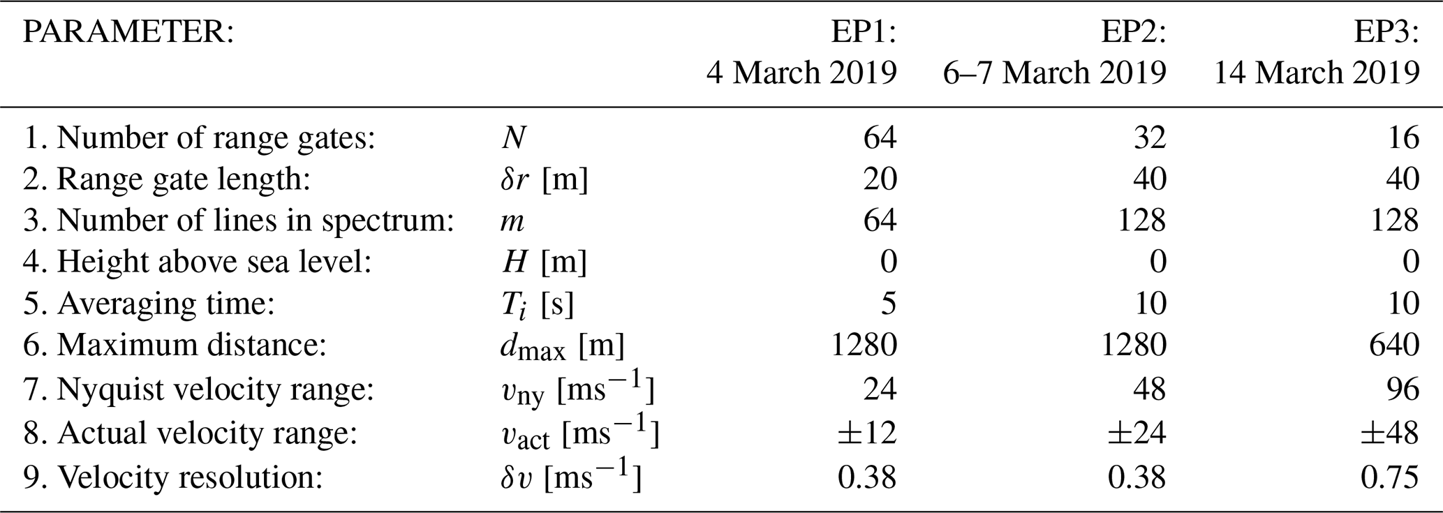
Different MRR parameter settings were tested during the RACLETS campaign to find the best setting for detecting blowing snow off mountain ridges. The most important parameters were those defining the distance and velocity resolution. Table 1 provides a brief overview of the MRR instrument configuration used in this study (more information in Maahn and Kollias, 2012 and MRR Pro Manual, 2016). It is possible to set the following five MRR configuration parameters: (i) the number of range gates N=32, 64, 128 or 256, where a range gate defines a measurement volume of a certain length in the MRR pointing direction; (ii) the range gate length δr (>10 m) (the maximum measurement distance dmax is thus defined by N×δr); (iii) the number of lines in spectrum m=32, 64, 128 or 256, which controls the velocity resolution; (iv) the height above sea level H of the MRR installation site (this parameter is used for assumptions to compute rain rate from spectral power; since it is not relevant for this study, it was set to 0); and (v) the averaging time Ti>1 s of the power spectra defining the temporal resolution of the MRR products (MRR Pro Manual, 2016).
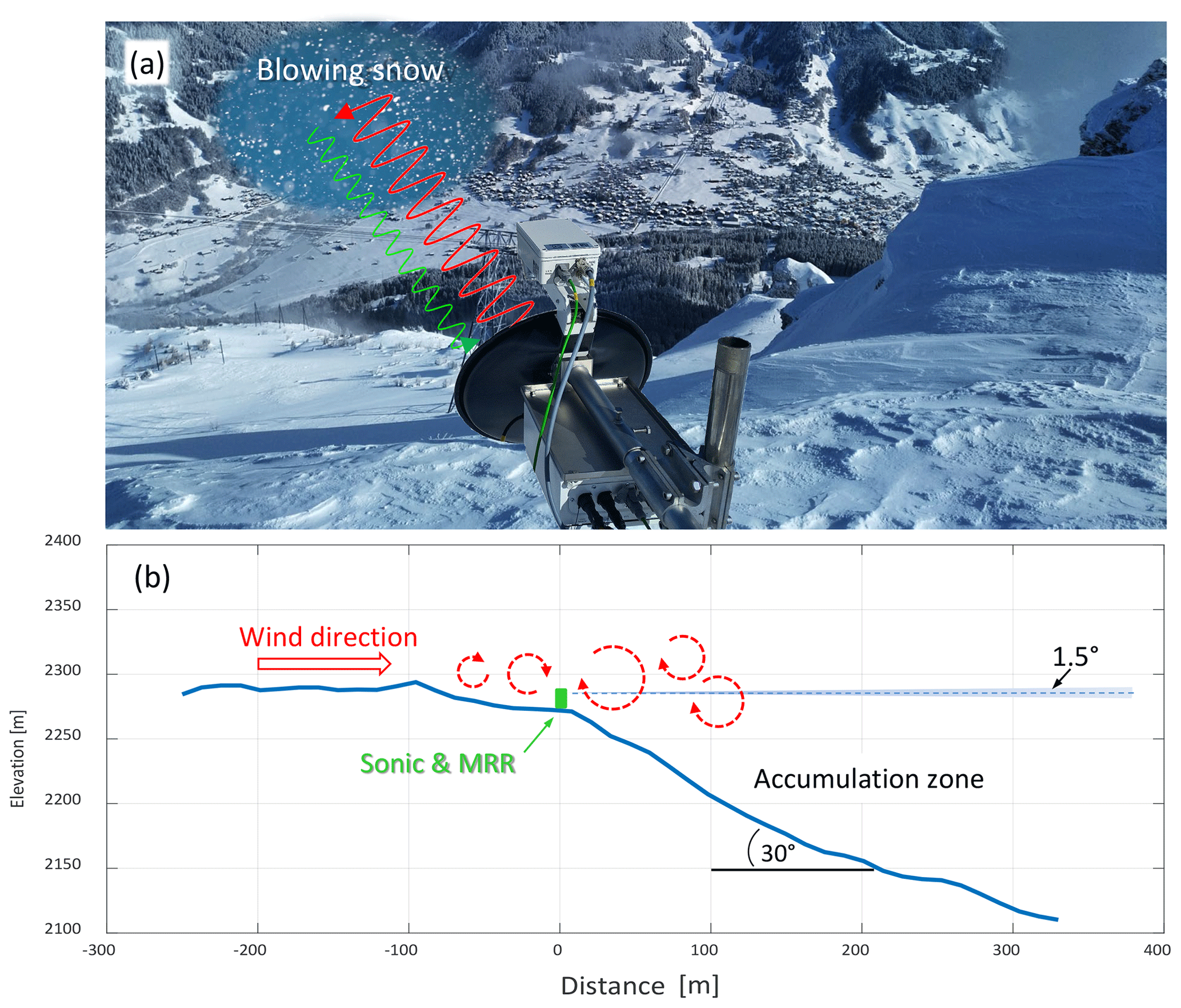
Figure 1(a) Picture of the study site: the Micro Rain Radar (MRR) is looking horizontally from the ridge, measuring the radial velocity and distance of blowing snow clouds across the valley. (b) Transect of the topography in the viewing direction of the MRR (aspect ratio is 1:1).
The first range gate was removed for the analysis, since it is affected by near-field effects. The first useable range gate covers the range 20 to 40 m, and the maximum measurement distance was m for EP1 on 4 March 2019 (Table 1). The half-power beam width of the MRR is 1.5∘, resulting in a beam expansion of about 1.3 m at 100 m. The Nyquist velocity range is inverse proportional to the number of range gates N (MRR Pro Manual, 2019) and was at the minimum for EP1 with vny=24 m s−1. The velocity resolution δv of the MRR radial velocity vMRR is given by vny∕m. Because the wind direction was expected to vary depending on the general weather situation, with snow potentially being blown either away or towards the MRR, the available velocity range vny was set symmetrically to 0, resulting in an actual velocity range (Table 1). Velocities of result in aliasing (Tridon et al., 2011) but can be corrected for by applying a dealiasing procedure based on , where n is the dealiasing number (integer of −1 if the lower limit of the Nyquist interval is exceeded and +1 if the upper limit is exceeded). However, particle velocities were rare. Another possible source of uncertainty for the Doppler velocity is the effect of ground clutter at small range gates, where the beam is not properly formed. However, since the MRR was installed at the edge of a steep slope (30∘, Fig. 1b), the effects of ground echoes on the measured Doppler velocity can be neglected. Furthermore, it is difficult to quantify an uncertainty on the mean Doppler velocity vMRR that is a moment of a distribution, the Doppler spectrum. The measure of the Doppler velocity itself is relatively precise; i.e. it depends on the precision of the clock in the radar. It is more uncertain to what extent the mean Doppler velocity is representative of the movement of the particles within a range gate. However, the main wind direction was typically well aligned with the MRR view direction, and the velocity fluctuations induced by turbulence is assumed to be normally distributed around the mean so that the mean Doppler velocity vMRR well represents the mean wind or particle velocity within a range gate. The averaging time was set to Ti=5 s for EP1 and Ti=10 s for EP2 and EP3.
Providing a recommendation for an ideal MRR parameter combination is difficult, as it depends on the transport distance and velocity of the blowing snow events. Based on the results of this study, we recommend starting with a number of (N=32) short (δr=10 m) range gates resulting in a high distance resolution, a typically sufficient maximum measurement distance of 320 m and a high Nyquist frequency of vny=48 m s−1 ( m s−1). A maximum possible value of m=256 for the number of lines in spectrum results in a high velocity resolution of δv=0.19 m s−1. An averaging time of Ti=5 s seems to result in a sufficient temporal resolution without producing too much data while still capturing the major flow variability.
Table 1MRR parameter settings (parameters 1–5) for the three different evaluation periods investigated and the resulting MRR limits (parameters 6–9):
Among the standard products of the METEK processed data, the mean MRR radial velocity vMRR and the spectrum width σv,MRR obtained for each averaging period Ti are of primary interest in the subsequent analysis, providing information on the blowing snow particle cloud velocities and turbulence intensities. Furthermore, the last range gate reflecting the MRR signal defines the blowing snow travel distance d in the MRR pointing direction for each averaging period Ti. Finally, the radar reflectivity Z, which mainly depends on the particle size, provides an indication of blowing snow particle sizes. The determination of blowing snow particle cloud concentrations and a mass flux is not possible, since there is no quantitative relationship between the spectral power and the particle size distribution for snow. Nevertheless, the MRR measurements provide other interesting characteristics of blowing snow events as discussed in the following sections.
The MRR was mounted at the edge of a few-hundred-metre-wide flat mountain ridge transitioning into a 30∘ slope defining the accumulation zone. A transect of the topography of the test site in the direction of the MRR's field of view (Fig. 2a) is shown in Fig. 1b. The MRR was oriented at an azimuth angle of 22∘ (clockwise with respect to north; see Fig. 2a). Note that the MRR radial velocity and turbulence characteristics determined from the MRR Doppler spectra are meant exclusively in the direction of the field of view of the MRR. However, the wind direction α was typically along the MRR pointing direction; thus the MRR radial velocity is typically close to the blowing snow absolute velocity.
At about 5 m from the MRR, sensors of the SDS were mounted on a mast. The present study uses measurements of the three wind components (u, v, w) and the wind direction (α) measured with a 3D ultra-sonic anemometer (R. M. Young 81000) at a height of 1.5 m above ground at a sampling frequency of 20 Hz.
Two drone flights were performed on 12 and 29 March 2019 with the SenseFly eBee+ RTK fixed-wing Unmanned Aerial System (UAS) to photogrammetrically map the local snow height changes due to pre- and post-depositional snow redistribution processes in between these measurements. Photogrammetric snow depth mapping with UAS has proven to be an accurate and reliable method if capturing the spatial variability in high alpine terrain with accuracies in the range of 5 to 30 cm (Bühler et al., 2016, 2017; Harder et al., 2016; Redpath et al., 2018). As a meaningful distribution of ground control points in the steep and dangerous slope was not possible, we applied integrated sensor orientation using the UAS GNSS measurements (mean positioning accuracy: 2.5 cm). This approach proved to be valid for accurate georeferencing (Benassi et al., 2017). This is also supported by several studies we performed for snow depth mapping applying ground control points (Bühler et al., 2018; Noetzli et al., 2019). For both flights we had a mean flight height above ground of 190 m resulting in a ground sampling distance (GSD) of about 4 cm. However, on 12 March 2019, wind gusts with high velocities up to 18 m s−1 occurred, which led to deviations of the plane along the flight lines, resulting in a reduced overlap of the imagery. Therefore, some photogrammetric noise is present in the resulting digital surface model (DSM), reducing its accuracy (Fig. 2a). No such noise is present in the data acquired on 29 March 2019, a day with calm wind conditions. We produced two 10 cm resolution DSMs and calculated the elevation difference by subtracting them (Fig. 2a).
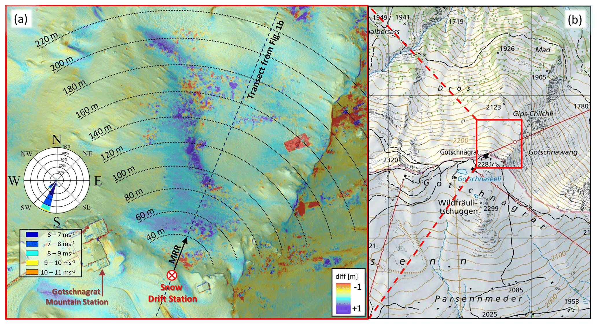
Figure 2Aerial view of the study domain close to the Gotschnagrat mountain station: (a) colours indicate the difference in snow height (diff) between 29 and 12 March 2019 determined from two photogrammetry drone flights, showing areas of up to 1 m of snow accumulation north of the snow drift station. The horizontally aligned MRR instrument is mounted at an azimuth angle of 22∘ at a height of about 1 m above ground. A wind rose indicates the wind speed and direction of all major wind events with a wind speed >6 m s−1 and thus potentially blowing snow effective for the period from 12:00 UTC+1 on 12 March 2019 to 12:00 UTC+1 on 21 March 2019. (b) Surrounding topography of the study site (Pixmap © 2020 swisstopo (5704000000), reproduced with permission of swisstopo (JA100118)).
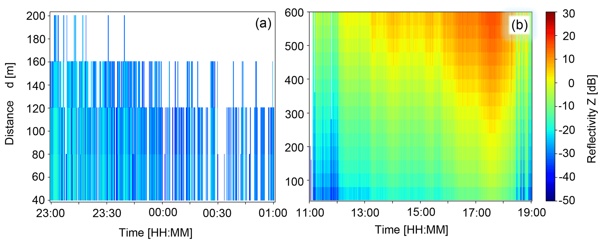
Figure 3MRR reflectivity for (a) part of EP2 (6–7 March 2019) for pure blowing snow events and (b) EP3 (14 March 2019) for blowing snow with concurrent snow precipitation.
3.1 The radar reflectivity
The radar reflectivity Z is proportional to the fourth power of the diameter for snow particles (Ryzhkov and Zrnic, 2019) and is thus mainly affected by the snow particle size and less so by the concentration as discussed before. The low reflectivity values of the measured pure blowing snow clouds (Fig. 3a), compared to the higher reflectivity of precipitation snowflakes (Fig. 3b), imply that the measured blowing snow clouds were composed of rather small particles. This is consistent with other findings of drifting and blowing snow investigations where small particle sizes of typically 50–500 µm were detected (Nishimura and Nemoto, 2005; Gromke et al., 2014) compared to precipitation snowflakes that can have diameters of several millimetres (e.g. Gergely et al., 2017). The lower reflectivities closer to the ridge (d=0–200 m) compared to further away (d>300 m) for the precipitation event (Fig. 3b) indicate smaller blowing snow particles due to higher wind speeds near the mountain ridge, whereas further away larger precipitation particles potentially dominate the backscatter of the radar signal.

Figure 4(a) MRR radial velocity in the azimuth direction 22∘ for a 2 min period containing four different blowing snow events on 4 March 2019. (b) Corresponding turbulence intensity I, Sonic (c) wind velocity (absolute and in the direction 202∘) and (d) turbulence intensity for 5 s intervals.
3.2 Radial velocity and turbulence intensity: exemplary cases
The MRR radial velocity vMRR (Eq. 2) within a range gate is computed as the average of the MRR Doppler spectrum (MRR Pro Manual, 2016) and is directly related to the blowing snow particle cloud velocity in the viewing direction of the MRR. In this section we introduce the basic MRR data by means of four exemplary blowing snow events (Fig. 4), including a brief discussion and interpretation of the results, as these data form the basis for the analyses presented in the following sections. Figure 4a shows the MRR radial velocity vMRR of the four blowing snow events of different characteristics within a 2 min time frame during EP1. The first event (no. 1) lasted for 25 s with a constant transport distance of 60 m. For the subsequent range gates (>60 m), no snow particles were in the field of view of the MRR anymore (Fig. 1b). The assumption is that the snow was blown off the ridge horizontally by up to about 60 m before it started settling, either resulting in local accumulation or being further advected closer to the ground, and thus leaving the field of view of the MRR. Event no. 1 started with relatively high MRR radial velocities of about vMRR=10–11 m s−1, while the velocities gradually decreased to about vMRR=7–8 m s−1 towards the end of this event. The Sonic wind velocities (Fig. 4c) are in good agreement, also decreasing to about vSonic=8 m s−1 towards the end of event no. 1. The turbulence intensity IMRR=0.06–0.12 of this first event (Fig. 4b) shows low-velocity fluctuations of the particle cloud, indicating a rather stable low-level, low-turbulence jet, which is supported by the Sonic turbulence intensities (Fig. 4d). The velocity drop at the end of event no. 1 is likely the reason for the break in snow being blown off the ridge between event nos. 1 and 2.
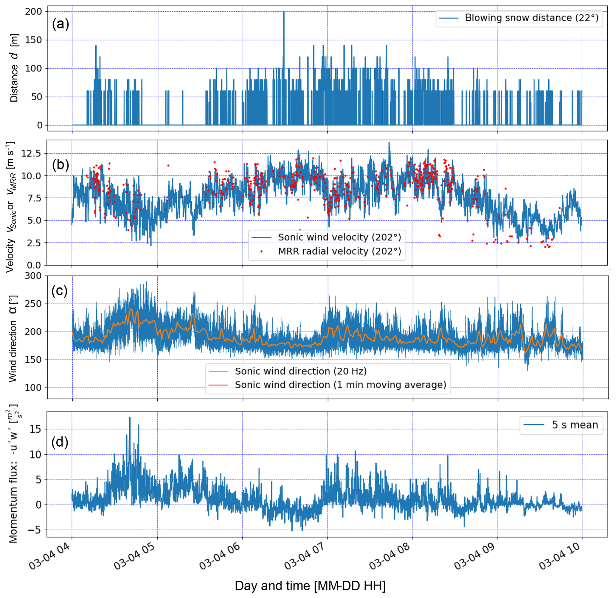
Figure 5(a) Temporal evolution of the horizontal transport distance of all blowing snow events of EP1 (4 March, 04:00–10:00 UTC+1). (b) Wind velocity parallel to the MRR direction (202∘) measured with the Sonic compared to the close range (20–40 m) blowing snow radial velocities measured with the MRR (see Fig. 4a). (c) Wind direction (mainly 180–220∘) and (d) momentum flux calculated using the Sonic data.
Blowing snow event no. 2 is different, starting with lower radial velocities of about vMRR=9 m s−1, likely initiated by higher wind velocities starting around 04:16:00 (Fig. 4c), and then suddenly dropping to about vMRR=6–7 m s−1 during the following 10 s because of another wind velocity vSonic decrease around 04:16:10 (Fig. 4c). Strong velocity changes are an indication of turbulent gusts, which is supported by higher MRR turbulence intensities of up to IMRR=0.27 (Fig. 4b). The maximum turbulence intensity at the SDS measured with the Sonic in the direction of the MRR was ISonic=0.25 (Fig. 4d) and thus in good agreement with the MRR result. However, the temporal agreement of the peak turbulence intensity is rather poor, as the peak in ISonic lags the peak in IMRR although it should be vice versa. Nevertheless, an overall good agreement between the turbulence intensities measured with the Sonic and that of the first range gate of the MRR is found, with a mean difference of ΔI= mean ( with standard deviation of σΔI=0.09 for the entire EP1 and EP2. The lower-velocity particle cloud of event no. 2 is transported further within the field of view of the MRR compared to event no. 1, resulting in a gradually increasing transport distance starting from 60 and increasing to 80, 120 and finally 140 m after 20 s. Interestingly, vMRR increases with distance for event no. 2, which is counter-intuitive, as one would rather expect a decrease of the wind velocity behind the ridge. However, the highly turbulent flow with changes in the wind direction and potentially large eddies of up to 100 m is likely causing this effect of higher velocities at longer distances. Event nos. 3 and 4 both show rather high radial velocities similarly to event no. 1, which are in good agreement with the Sonic wind velocities (Fig. 4c), but with slightly higher turbulence intensities, indicating a more turbulent flow unlike for event no. 1. The transport distances are about 80–100 m for event nos. 3 and 4.
Based on the above discussion of the four blowing snow events, it seems that stronger turbulent fluctuations with higher turbulence intensities result in longer transport distances. This leads us to the hypothesis that not necessarily low-turbulence jets with high wind velocities but turbulent gusts with lower wind velocities may be more effective in transporting blowing snow over longer distances on the lee side of a mountain ridge. Another explanation could be that the blowing snow cloud is vertically more extended for turbulent gusts, which increases the likelihood of snow particles being in the field of view of the MRR (Fig. 1b), whereas for low-level, low-turbulence jets the particles may rather quickly settle after a certain distance, leaving the field of view of the MRR. These considerations are further discussed in Sect. 3.4.
3.3 Blowing snow distances
The MRR blowing snow distances d for EP1 are shown in Fig. 5a. Typically, a minimum distance of about 60 m is reached, whereas longer distances >100 m appear rather seldom. The distances d and particle cloud radial velocities vMRR (Fig. 5b) may be smaller than the real absolute distances and velocities, as blowing snow was detected from various angles (Fig. 5c), not only straight in the view direction of the MRR as mentioned earlier. Nevertheless, the main wind direction was typically in overall good agreement with the view direction (202∘) of the MRR (Fig. 5c), and the main interest of this study is in snow being blown off perpendicular to the Gotschnagrat mountain ridge. A comparison between the MRR radial velocities vMRR of the first useable range gate (d=40 m) and the horizontal wind velocity vSonic measured with the Sonic, both for the direction of 202∘, is provided in Fig. 5b. A qualitatively good agreement is found despite some outliers. Very low MRR velocities around vMRR=2.5 m s−1 are either an instrument artefact because of very low blowing snow particle concentrations or else caused by wind directions temporarily deviating significantly from the MRR field-of-view direction. Discrepancies between the MRR and the Sonic velocities may be the result of the spatial average distance of about 30 m between the first usable range gate d=40 m (with a measurement volume extending from 20 to 40 m) and the location of the Sonic in combination with the slightly varying wind direction. To assess a potential dependency of the velocity difference on the wind direction, Fig. 6 shows the relative difference between the MRR and the Sonic velocity as a function of the wind direction α for EP1–EP3. A positive trend is found with a bias of vMRR>vSonic for wind directions α>180∘. Nevertheless, an overall good agreement between the MRR radial and Sonic velocity is found, with a mean difference of mean % and a standard deviation of ±20 %. The intersection of the linear fit with the line for α=170∘ (Fig. 6) suggests a stable wind direction in the vicinity of the MRR and the SDS for winds coming from that direction. This result is most likely strongly related to the local topography (Fig. 2b) influencing the nearby wind field and direction, where the mountain station is located west and another SW–NE-oriented mountain ridge east of the MRR and the SDS, resulting in a rather undisturbed flow for southerly winds.
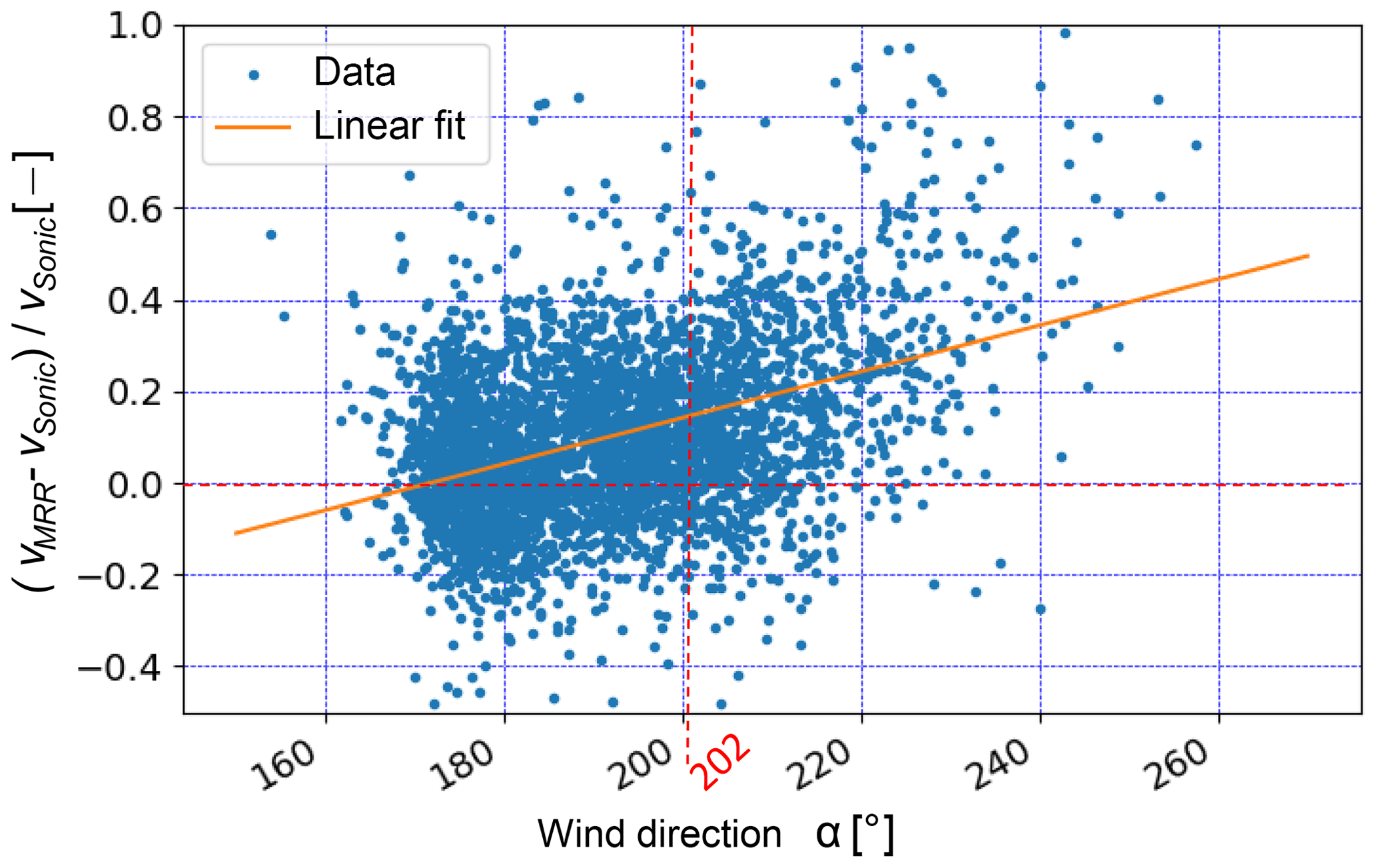
Figure 6Relative difference between MRR and Sonic wind velocity in the direction 202∘ as a function of wind direction for EP1–EP3.
Figure 5d shows the momentum flux calculated from the Sonic wind velocities, which is generally positive for EP1, indicating a downward momentum flux and an increase in wind velocity with height above the location of the Sonic. However, between 06:15 and 07:00 UTC+1, the momentum flux was negative, indicating a decreasing wind velocity with height above the Sonic and the presence of a low-level jet close to the ground constantly blowing from a direction of 180∘ (south). During this time period, the wind velocity was highest, at up to 12–13 m s−1, and long blowing snow distances were reached of typically >80 m (Fig. 5a). Furthermore, the best agreement between the Sonic wind velocity and the MRR radial velocity was found for this period of stable wind conditions.
Very similar results were found for EP2 (Fig. 7). Longer transport distances (Fig. 7a) were typically obtained as a result of the higher wind velocities (Fig. 7b). The wind direction (Fig. 7c) was typically quite stable, although there were two periods (21:00–22:00 and 23:00–23:30 UTC+1) where the wind direction varied significantly. The momentum flux (Fig. 7d) was negative about 50 % of the time, indicating a higher presence of low-level jets close to the ground compared to EP1.
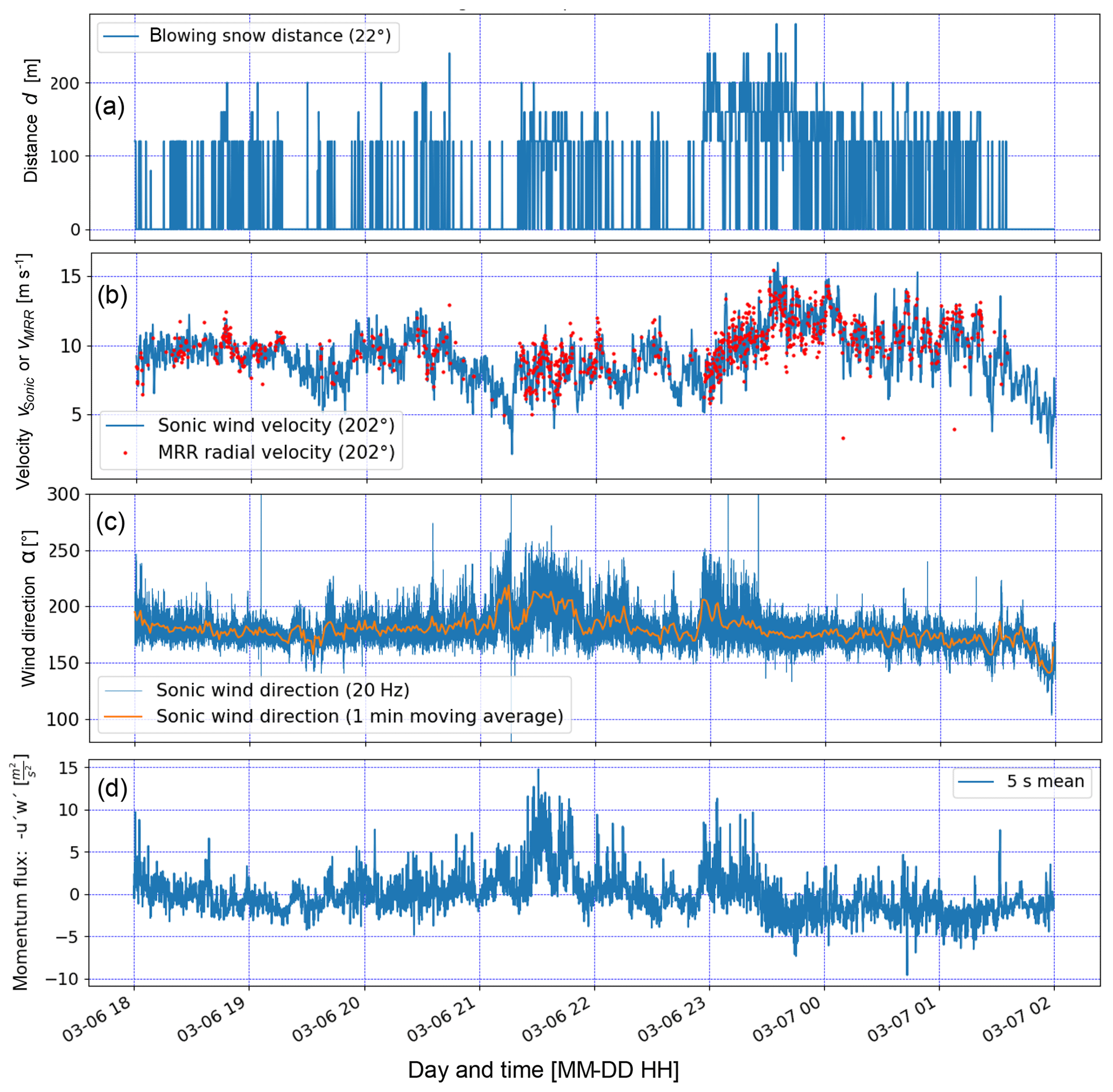
Figure 7(a) Temporal evolution of the horizontal transport distance of all blowing snow events of EP2 (18:00 UTC+1 on 6 March 2019 to 02:00 UTC+1 on 7 March 2019). (b) Wind velocity parallel to the MRR direction (202∘) measured with a Sonic compared to the close range (40–80 m) blowing snow radial velocities measured with the MRR. (c) Wind direction (mainly 180–220∘) and (d) momentum flux calculated using the Sonic data.
3.4 Blowing snow statistics
The relative frequency of occurrence of blowing snow transport distances from Fig. 5a is shown in Fig. 8a for EP1. Eighty percent of the time, no blowing snow was present or detected by the MRR (transport distance d=0 m). No events were detected for a distance d=20 m since this range gate cannot be used as discussed earlier. Only few events were detected for a transport distance d=40 m, although this range gate delivered continuous information on radial velocities for higher transport distances d>40 m (Fig. 4a). Therefore, we expect that also for d=20 m only very few or no events would have been detected by the MRR, resulting in a gap in the frequency distribution for m in Fig. 8a. We hypothesize that, if the wind is strong enough and above a threshold wind speed to entrain and transport snow in suspension, a minimum transport distance of d=60 m is reached, which occurred for about 10 % of the total time of observation for EP1 (including the “no blowing snow” time). For distances d>60 m, the relative frequency decreases exponentially, with the maximum distance of d=200 m only observed once. The mean Sonic wind velocity was 7.3 m s−1 during EP1, which is only 6 h long but sampled at a temporal resolution of 5 s, resulting in 4320 samples and thus providing a good data basis for statistics.
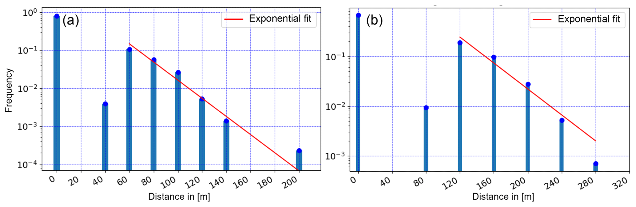
Figure 8Histogram of the transport distance of all blowing snow events for (a) EP1 (Fig. 5a) and (b) EP2 (Fig. 7a), including exponential fits for distances larger than the minimal transport distance.
The relative frequency of occurrence of blowing snow distances for EP2 (18:00 UTC+1 on 6 March 2019 to 02:00 UTC+1 on 7 March 2019) is shown in Fig. 8b. The mean wind velocity of 9.1 m s−1 during the 8 h (10 s sampling) measured with the Sonic was significantly higher compared to EP1 (7.3 m s−1), resulting in a larger gap before the minimal transport distance and higher overall transport distances of up to maximum d=280 m. The higher minimal transport distance of d=120 m compared to EP1 might be the result of stronger gusts during the more powerful storm of EP2 and the conditions and erodibility of the snow surface. Despite some differences between the two distributions in Fig. 8, both show very similar characteristics, with a gap before a minimal distance is reached and an exponential decay afterwards. Therefore, those distributions seem to be generally valid, providing a good representation of the frequency of blowing snow distances for mountain ridges. A dependency of the minimal transport distance and the frequency distribution on the strength of the storm event and snow cover conditions could be investigated in future more detailed studies.
To estimate a threshold wind velocity (e.g. Li and Pomeroy, 1997) and thus the erodibility of the surrounding snow surface, box plots of the Sonic wind velocity as a function of the transport distance are provided in Fig. 9. The median wind velocity increases by about 2 m s−1 for transport distances increasing from d=40 to 200 m for EP1 and about 5 m s−1 (d=80–280 m) for EP2. An extrapolation of the wind velocity to d=0 m provides an estimate of a threshold velocity of 7.5 m s−1 for EP1and 8.8 m s−1 for EP2, a result that is in overall good agreement with other studies (e.g. Li and Pomeroy, 1997). Note that the wind velocity threshold definition for particle transport used in this study, defined for a height of 1.5 m (Sonic), is similar to that used in Li and Pomeroy (1997), who defined a threshold wind speed at 10 m above ground. These definitions are different to the traditional definition of a threshold friction velocity for particle entrainment and saltation (e.g. Schmidt, 1980; Guyomarc'h and Mérindol, 1998; Clifton et al., 2006; Walter et al., 2012). The fact that the estimated threshold for EP2 (Fig. 9b) is 1.3 m s−1 higher than for EP1 (Fig. 9a) supports our previous hypothesis of different snow surface conditions with a reduced erodibility for EP2.
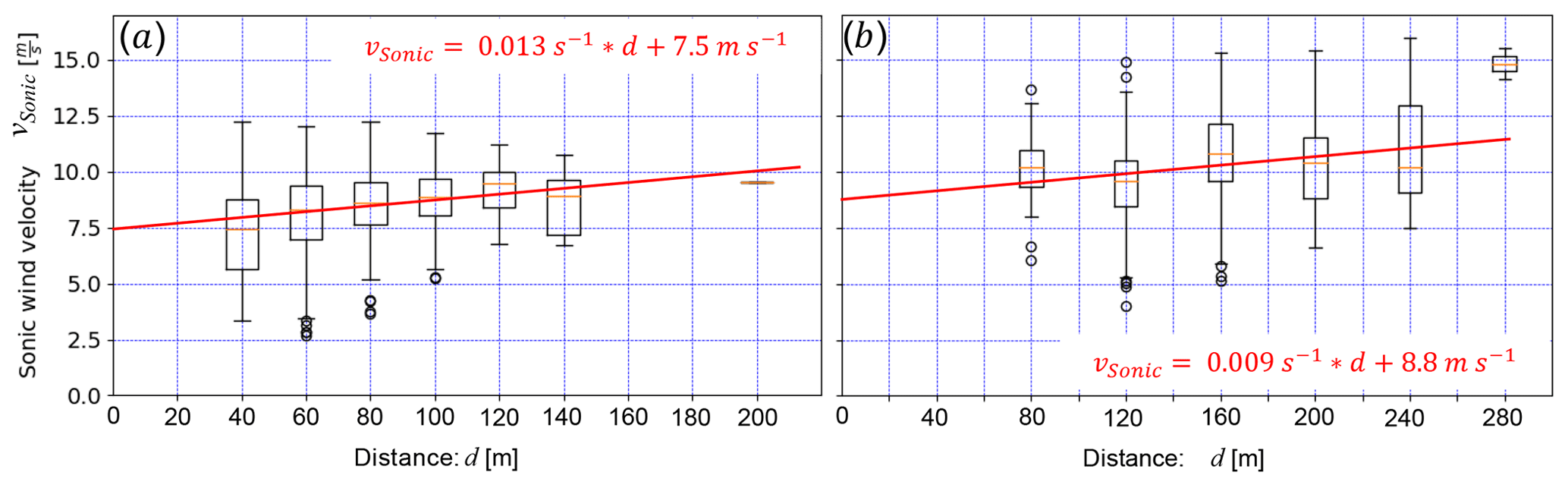
Figure 9Sonic wind velocity as a function of the transport distance of the blowing snow events for (a) EP1and (b) EP2.
Turbulent gusts at rather low velocities were found to be potentially responsible for longer transport distances as discussed in Sect. 3.2 (Fig. 4a). To investigate whether these events or low-level, low-turbulence jets with high wind velocities are more effective in transporting snow over long distances across a mountain ridge, the turbulence intensities of the last range gate defining the blowing snow transport distance (Fig. 4b) are plotted as a function of the transport distance (box plot) in Fig. 10. For EP1 (Fig. 10a) and distances d≥80 m, the median, the upper and lower quartiles, the whiskers and the outliers all show a decreasing trend with increasing distance, indicating that low-level, low-turbulence jets with high wind velocities are more effective than highly turbulent gusts in transporting blowing snow over long distances across a mountain ridge for EP1. Nevertheless, as mentioned earlier, highly turbulent motions still may result in a higher vertical extension of blowing snow clouds and thus in an increased likelihood of being within the field of view of the MRR (Fig. 1b) for long distances. For the stronger storm event of EP2, the turbulence level was significantly higher, with median intensities of 0.1–0.2 (<0.5 for EP1) (Fig. 10b), supporting the latter assumption. Strong low-turbulence jets may also result in a slight downward air flow right after the ridge, and the blowing snow may quickly settle, thereby getting out of the field of view of the MRR. The turbulence statistics shown in Fig. 10 do thus not allow a conclusion to be drawn on whether low-level, low-turbulence jets or turbulent gusts are more effective in transporting blowing snow over longer distances. However, highly turbulent flows are more likely to bring particles to greater heights and thus influence cloud processes. Measurements with a two-MRR system oriented parallel at different heights could provide a conclusion on which of the two events is more effective in transporting snow over longer distances across mountain ridges.
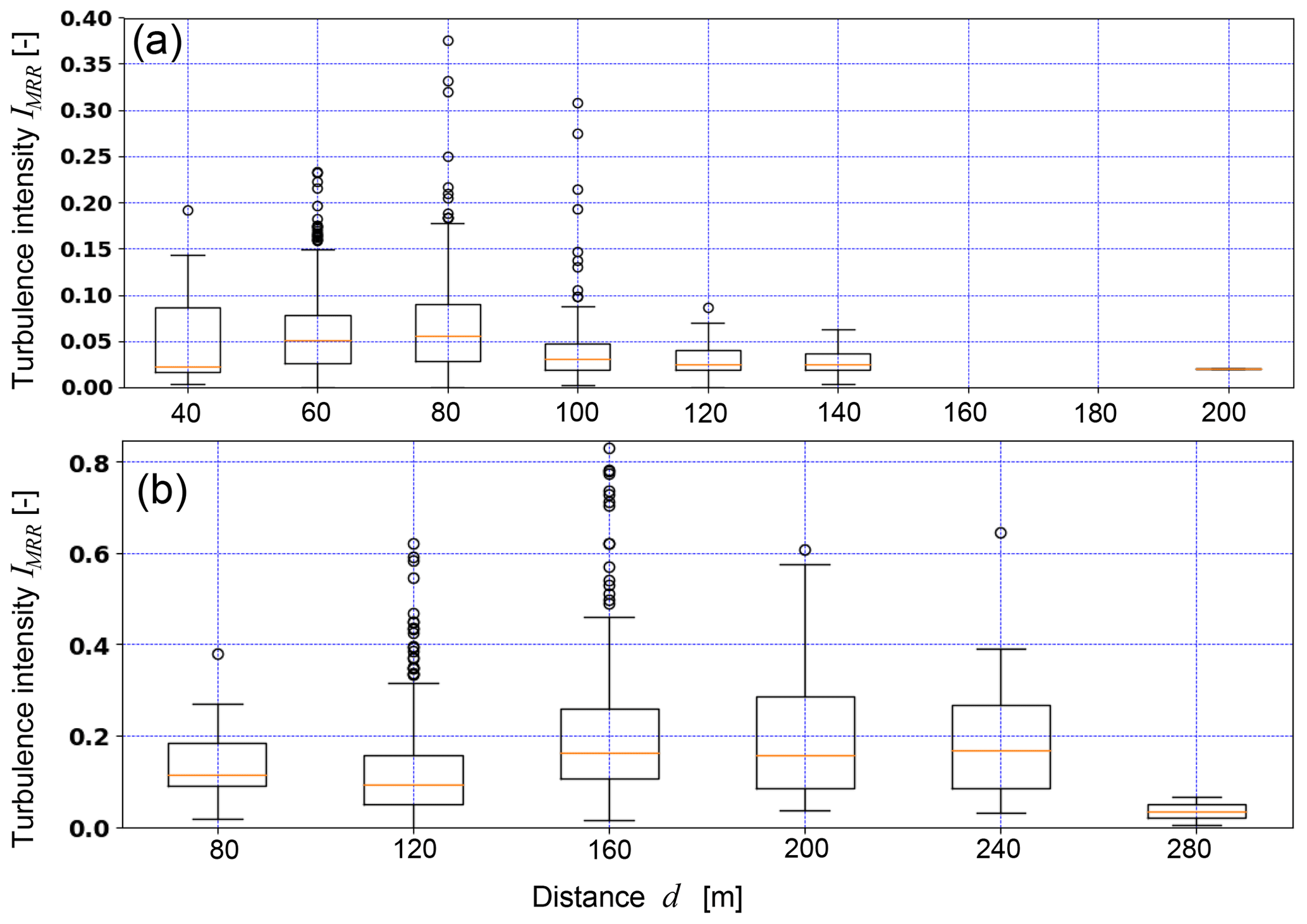
Figure 10Turbulence intensity determined from the MRR spectral width of the Doppler spectrum of the range gate defining the blowing snow transport distance (Fig. 4a) as a function of transport distance for (a) EP1 and (b) EP2.
3.5 Snow height distribution
To provide a first connection between mountain ridge blowing snow events and a subsequent snow height distribution in the vicinity, the measured snow height distribution (Fig. 2a) is discussed in the context of prevailing precipitation and wind conditions and related to the analysed blowing snow events in this section. The spatial variation in snow height difference between 29 and 12 March 2019 of the investigated area around the MRR (Fig. 2a) shows distinct patterns as a result of pre- and post-depositional accumulation and erosion processes. Deep blue and deep red spotted areas of maximum snow depth differences are an artefact from wind gusts affecting the drone flights on 12 March 2019, resulting in erroneous photogrammetry measurements (see Sect. 2). Nevertheless, the smooth areas of the snow depth map show that significant snow deposition occurred north of the SDS in between the two drone flights, while other regions were eroded.
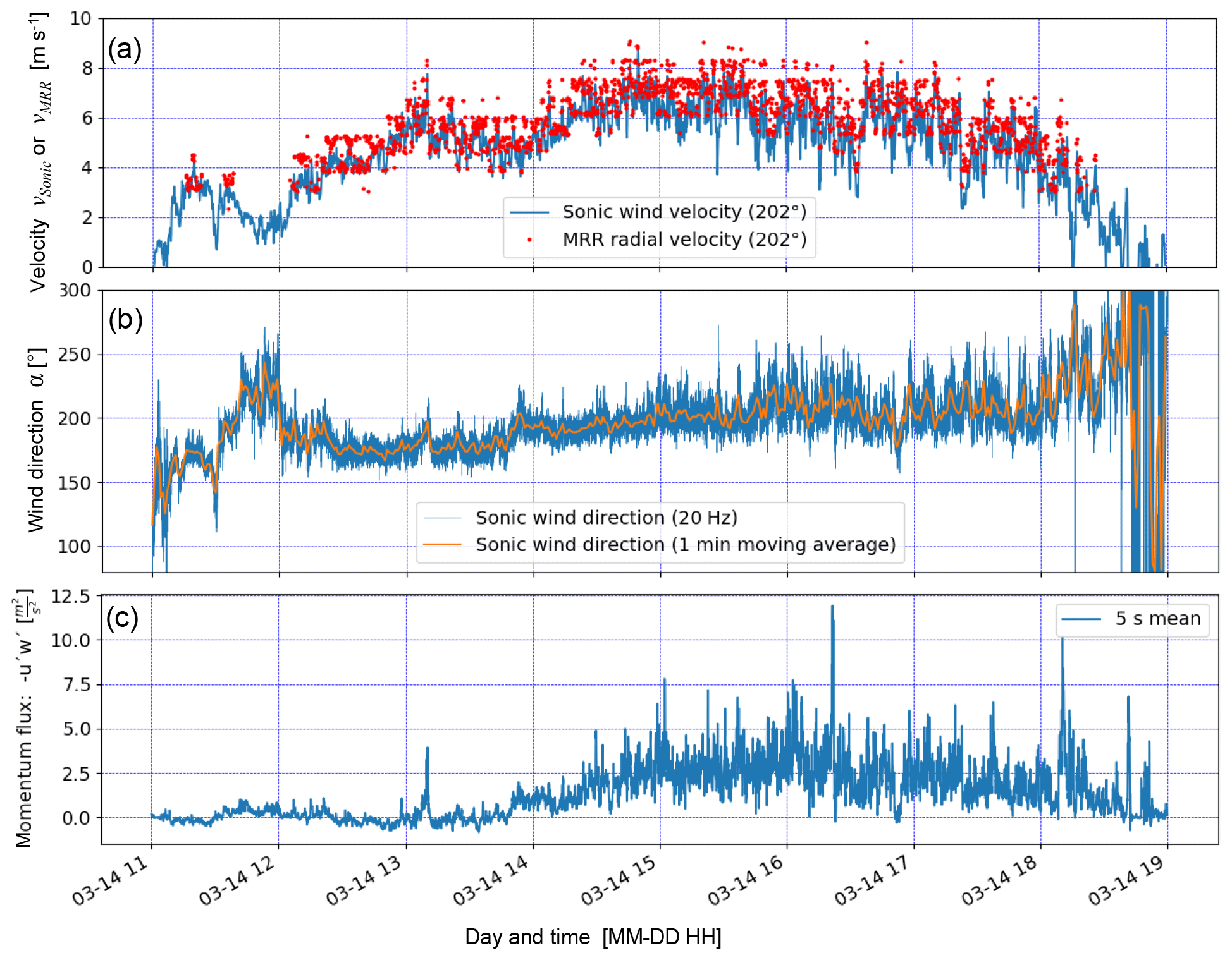
Figure 11Precipitation event (EP3) on 14 March 2019 with strong wind from the south resulting in blowing snow and preferential deposition north of the snow drift station as shown in Fig. 2a. (a) Sonic wind velocity and MRR radial velocity, (b) wind direction and (c) momentum flux calculated using the Sonic data (similar to Figs. 5 and 7).
The increased snow accumulation north of the MRR shown in Fig. 2a is the result of a combination of preferential deposition and blowing snow, i.e. pre- and post-depositional accumulation processes. Although the pure blowing snow events analysed in the previous sub-sections took place about a week prior to this long-term observational period between the two drone flights, two major snow storm events were found to be responsible for the accumulation during the 17 d between the two flights on 12 and 29 March 2019. Figure 11a shows a comparison of the Sonic wind velocity and the MRR radial velocity (similar to Figs. 5b and 7b) for the first precipitation event on 14 March 2019 (EP3). For this precipitation event, the MRR particle velocities are also in good agreement with the Sonic wind velocity at levels of up to 8 m s−1, similar to those of the pure blowing snow events of EP1 and EP2. The wind direction was also well aligned with the MRR view axis and quite stable from S to SW (approx. 200∘) for the entire storm (Fig. 11b). We assume that the wind resulted not only in preferential deposition during the precipitation event but also in snow on the ground being entrained and transported during strong gusts from the ridge to the accumulation zone (Figs. 1b, 2a). This simultaneous appearance of pre- and post-depositional accumulation processes also occurred during the second snow storm on 15 March 2019, which was very similar but is not presented here. The wind rose shown in Fig. 2a summarizes the wind directions for wind velocities >6 m s−1, thus potentially blowing snow effectively, for the 9 d period 12 to 21 March 2019. On the last day, the MRR and the instruments of the SDS were dismantled. However, although the wind rose does not cover the entire period between the two drone flights, it clearly shows that the blowing snow effective wind direction was stable from S to SW at least for the first half of the time between the two drone flights. Similar transport distances for the blowing snow events with concurrent precipitation (EP3) to those without (EP1 and EP2) are assumed, based on the similarity of the wind direction and wind velocity. Therefore, the increased accumulation north of the ridge up to distances of 200 m (Fig. 2a) are very likely the result of the two blowing snow events with concurrent precipitation between the two drone flights. Although the wind velocities for EP3 (Fig. 11a) are slightly smaller than for EP1 and EP2, probably resulting in smaller transport distances than shown in Figs. 5a and 7a, the snow likely gets transported closer to the ground outside the field of view of the MRR before it is finally deposited, which might explain increased accumulation for distances of up to d=220 m (Fig. 2a). Although the local topography and the near-ground wind velocities north of the ridge also influenced the small-scale (metres) snow height distribution on the ground, the main conclusion is that an overall good agreement is found between the blowing snow direction, wind velocities, blowing snow distances and larger-scale (several tens of metres) snow accumulation pattern.
Our results show that radar measurements of blowing snow may deliver valuable information to improve our understanding of pre- and post-depositional snow accumulation or redistribution processes on larger scales. The Micro Rain Radar (MRR) instrument provides characteristics of and statistics on blowing snow distances, its frequency of occurrence, particle cloud velocities and turbulence intensities. We found good agreement between the MRR blowing snow velocity and the Sonic wind velocity, and that a minimal horizontal blowing snow transport distance of 60–120 m is reached in the lee of a mountain ridge, depending on the strength of the storm event. The relative frequency of occurrence decreases exponentially for distances longer than the minimal transport distance, with a measured maximum distance of 280 m in our case. It was not possible to draw a conclusion on whether low-level, low-turbulence jets or turbulent gusts are more effective in transporting blowing snow over longer distances in the lee of a mountain ridge. The increased snow height distribution north of the measurement location (Fig. 2a) was found to be the result of a combination of preferential deposition and blowing snow accumulation during at least two measured and analysed snowstorm events. The presented snow height distributions together with the characterization of the blowing snow events provide a valuable data basis for validating coupled numerical weather and snowpack simulations.
Further investigations are required for more clarification and may incorporate measurements with a second MRR system oriented parallel at a slightly different elevation to better resolve the local wind field and blowing snow events – particularly to capture the process of settling snow disappearing from the field of view of the upper MRR. The MRR instrument was also recently tested by the Cryos group at EPFL, Lausanne, Switzerland, for measuring vertical velocity profiles and temporal variability of blowing snow in East Antarctica at the site S17 near the Japanese research station Syowa (unpublished work in progress), where blowing snow layers can reach a vertical extent of up to 200 m (Palm et al., 2017). The next challenge for radar specialists will be finding a way to extract particle concentrations from the radar measurements to estimate particle mass fluxes or at least order of magnitude. Exploring the potential of horizontally pointing cloud physics lidar (e.g. Mona et al., 2012) in detecting the spatio-temporal variability of blowing snow would be worthwhile for the community interested in characterizing and better understanding pre- and post-depositional snow accumulation processes in various cold regions worldwide.
The MRR and SDS data for the entire RACLETS campaign are available on the ENVIDAT data repository (Walter and Huwald, 2019; Walter et al., 2019).
BW, HH and ML designed the experiments, and BW carried them out. JG provided MRR support, and YB conducted the drone flights. BW prepared the manuscript with contributions from all co-authors.
The authors declare that they have no conflict of interest.
We would like to thank the SLF workshop for supporting us with the design and construction of the snow drift station. Furthermore, we would like to thank the Environmental Remote Sensing Laboratory (LTE) at EPFL, especially Alexis Berne and Alfonso Ferrone for lending the MRR and for the technical support with the instrument. Thanks also to Andreas Stoffel, Elisabeth Hafner and Lucie Eberhard for performing the photogrammetric drone flights; David Wagner, Felix von Rütte and Beat Nett for their support with the installation of the snow drift station; and Rebecca Mott for the GIS support.
This research has been supported by the Swiss National Science Foundation (grant no. 200020-179130 and 200020-175700/1).
This paper was edited by Guillaume Chambon and reviewed by Michele Guala and one anonymous referee.
Aksamit, N. O. and Pomeroy, J. W.: Near-surface snow particle dynamics from particle tracking velocimetry and turbulence measurements during alpine blowing snow storms, The Cryosphere, 10, 3043–3062, https://doi.org/10.5194/tc-10-3043-2016, 2016.
Armstrong, R. L. and Brun, E.: Snow and Climate: Physical Processes, Surface Energy Exchange and Modeling, Cambridge University Press, 222 pp., 2008.
Bagnold, R. W.: The Physics of Blown Sand and Desert Dunes. Methuen, London, 1941.
Benassi, F., Dall'Asta, E., Diotri, F., Forlani, G., Morra di Cella, U., Roncella, R. and Santise, M.: Testing Accuracy and Repeatability of UAV Blocks Oriented with GNSS-Supported Aerial Triangulation, Remote Sensing, 9, 172, https://doi.org/10.3390/rs9020172, 2017.
Beniston, M., Farinotti, D., Stoffel, M., Andreassen, L. M., Coppola, E., Eckert, N., Fantini, A., Giacona, F., Hauck, C., Huss, M., Huwald, H., Lehning, M., López-Moreno, J.-I., Magnusson, J., Marty, C., Morán-Tejéda, E., Morin, S., Naaim, M., Provenzale, A., Rabatel, A., Six, D., Stötter, J., Strasser, U., Terzago, S., and Vincent, C.: The European mountain cryosphere: a review of its current state, trends, and future challenges, The Cryosphere, 12, 759–794, https://doi.org/10.5194/tc-12-759-2018, 2018.
Bühler, Y., Adams, M. S., Bösch, R., and Stoffel, A.: Mapping snow depth in alpine terrain with unmanned aerial systems (UASs): potential and limitations, The Cryosphere, 10, 1075–1088, https://doi.org/10.5194/tc-10-1075-2016, 2016.
Bühler, Y., Adams, M., Stoffel, A., and Boesch, R.: Photogrammetric reconstruction of homogenous snow surfaces in alpine terrain applying near infrared UAS imagery, Int. J. Remote Sens., 38, 3135–3158, https://doi.org/10.1080/01431161.2016.1275060, 2017.
Bühler, Y., Stoffel, A., Eberhard, L., Feuerstein, G. C., Lurati, D., Guler, A., and Margreth, S.: Drohneneinsatz für die Kartierung der Schneehöhenverteilung, Bündnerwald, 71, 20–24, 2018.
Clifton, A., Rüedi, J. D., and Lehning, M.: Snow saltation threshold measurements in a drifting-snow wind tunnel, J. Glaciol., 52, 585–596, https://doi.org/10.3189/172756506781828430, 2006.
Comola, F., Giometto, M. G., Salesky, S. T., Parlange, M. B., and Lehning, M.: Preferential deposition of snow and dust over hills: Governing processes and relevant scales, J. Geophys. Res.-Atmos., 124, 7951–7974, https://doi.org/10.1029/2018JD029614, 2019.
Dadic, R., Mott, R., Lehning, M., and Burlando, P.: Wind influence on snow depth distribution and accumulation over glaciers, J. Geophys. Res. 115, F01012, https://doi.org/10.1029/2009JF001261, 2010.
Föhn, P. M.: Snow transport over mountain crests, J. Glaciol., 26, 469–480, 1980.
Geerts, B., Pokharel, B., and Kristovich, D. A.: Blowing snow as a natural glaciogenic cloud seeding mechanism, Mon. Weather Rev., 143, 5017–5033, 2015.
Gerber, F., Lehning, M., Hoch, S. W., and Mott, R.: A close-ridge small-scale atmospheric flow field and its influence on snow accumulation, J. Geophys. Res.-Atmos. 122, 7737–7754, https://doi.org/10.1002/2016JD026258, 2017.
Gerber, F., Besic, N., Sharma, V., Mott, R., Daniels, M., Gabella, M., Berne, A., Germann, U., and Lehning, M.: Spatial variability in snow precipitation and accumulation in COSMO–WRF simulations and radar estimations over complex terrain, The Cryosphere, 12, 3137–3160, https://doi.org/10.5194/tc-12-3137-2018, 2018.
Gerber, F., Mott, R., and Lehning, M.: The importance of near-surface winter precipitation processes in complex alpine terrain, J. Hydrometeorol., 20, 177–196, https://doi.org/10.1175/JHM-D-18-0055.1, 2019.
Gergely, M., Cooper, S. J., and Garrett, T. J.: Using snowflake surface-area-to-volume ratio to model and interpret snowfall triple-frequency radar signatures, Atmos. Chem. Phys., 17, 12011–12030, https://doi.org/10.5194/acp-17-12011-2017, 2017.
Gromke, C., Horender, S., Walter, B., and Lehning, M.: Snow particle characteristics in the saltation layerm, J. Glaciol., 60, 431–439, https://doi.org/10.3189/2014JoG13J079, 2014.
Groot Zwaaftink, C. D., Löwe, H., Mott, R., Bavay, M., and Lehning, M.: Drifting snow sublimation: A high-resolution 3-D model with temperature and moisture feedbacks, J. Geophys. Res., 116, D16107, https://doi.org/10.1029/2011JD015754, 2011.
Grünewald, T., Wolfsperger, F., and Lehning, M.: Snow farming: conserving snow over the summer season, The Cryosphere, 12, 385–400, https://doi.org/10.5194/tc-12-385-2018, 2018.
Guyomarc'h, G. and Mérindol, L.: Validation of an application for forecasting blowing snow, Anna. Glaciol., 26, 138–143, 1998.
Guyomarc'h, G., Bellot, H., Vionnet, V., Naaim-Bouvet, F., Déliot, Y., Fontaine, F., Puglièse, P., Nishimura, K., Durand, Y., and Naaim, M.: A meteorological and blowing snow data set (2000–2016) from a high-elevation alpine site (Col du Lac Blanc, France, 2720 m a.s.l.), Earth Syst. Sci. Data, 11, 57–69, https://doi.org/10.5194/essd-11-57-2019, 2019.
Harder, P., Schirmer, M., Pomeroy, J., and Helgason, W.: Accuracy of snow depth estimation in mountain and prairie environments by an unmanned aerial vehicle, The Cryosphere, 10, 2559–2571, https://doi.org/10.5194/tc-10-2559-2016, 2016.
Hong, J., Toloui, M., Chamorro, L. P., Guala, M., Howard, K., Riley, S., Tucker J., Sotiropoulos, F.: Natural snowfall reveals large-scale flow structures in the wake of a 2.5-MW wind turbine, Nat. Commun., 5, 4216, https://doi.org/10.1038/ncomms5216, 2014.
Kneifel, S., Maahn, M., and Peters, G.: Observation of snowfall with a low-power FM-CW K-band radar (Micro Rain Radar), Meteorol. Atmos. Phys., 113, 75–87, https://doi.org/10.1007/s00703-011-0142-z, 2011.
Lehning, M., Löwe, H., Ryser, M., and Raderschall, N.: Inhomogeneous precipitation distribution and snow transport in steep terrain, Water Resour. Res., 44, W07404, https://doi.org/10.1029/2007WR006545, 2008.
Li, L. and Pomeroy, J. W.: Estimates of threshold wind speeds for snow transport using meteorological data, J. Appl. Meteorol., 36, 205–213, 1997.
Maahn, M. and Kollias, P.: Improved Micro Rain Radar snow measurements using Doppler spectra post-processing, Atmos. Meas. Tech., 5, 2661–2673, https://doi.org/10.5194/amt-5-2661-2012, 2012.
Mona, L., Liu, Z., Müller, D., Omar, A., Papayannis, A., Pappalardo, G., Sugimoto, N., and Vaughan, M.: Lidar Measurements for Desert Dust Characterization: An Overview, Adv. Meteorol., 2012, 356265, https://doi.org/10.1155/2012/356265, 2012.
Moore, G. W. K.: Mount Everest snow plume: A case study, Geophys. Res. Lett., 31, L22102, https://doi.org/10.1029/2004GL021046, 2004.
Mott, R., Scipión, D. E., Schneebeli, M., Dawes, N., Berne, A., and Lehning, M.: Orographic effects on snow deposition patterns in mountainous terrain, J. Geophys. Res.-Atmos., 119, 1419–1439, https://doi.org/10.1002/2013JD019880, 2014.
Mott, R., Vionnet, V., and Grünewald, T.: The Seasonal Snow Cover Dynamics: Review on Wind-Driven Coupling Processes, Front. Earth Sci., 6, 197, https://doi.org/10.3389/feart.2018.00197, 2018.
MRR Pro Manual: Micro Rain Radar MRR Pro Manual, Meteorologische Messtechnik GmbH (METEK), Elmshorn, Germany, 2016.
Naaim-Bouvet, F., Bellot, H., and Naaim, M.: Back analysis of drifting-snow measurements over an instrumented mountainous site, Ann. Glaciol., 51, 207–217, https://doi.org/10.3189/172756410791386661, 2010.
Nishimura, K. and Nemoto, M.: Blowing snow at Mizuho station, Antarctica, Philos. T. R. Soc. A., 363, 1647–1662, https://doi.org/10.1098/rsta.2005.1599, 2005.
Nishimura, K., Yokoyama, C., Ito, Y., Nemoto, M., Naaim-Bouvet, F., Bellot, H., and Fujita, K.: Snow particle velocities in drifting snow, J. Geophys. Res.-Atmos., 119, 9901–9913, https://doi.org/10.1002/2014JD021686, 2014.
Nishimura, K., Nemoto, M., Okaze, T., and Niiya, H.: Investigation of the spatio-temporal variability of blowing snow, IUGG General Assembly, Montreal, 8–18 July 2019.
Noetzli, C., Bühler, Y., Lorenzi, D., Stoffel, A., and Rohrer, M.: Schneedecke als Wasserspeicher – Drohnen können helfen, die Abschätzungen der Schneereserven zu verbessern, Wasser, Energie, Luft, 111, 153–157, 2019.
Palm, S. P., Kayetha, V., Yang, Y., and Pauly, R.: Blowing snow sublimation and transport over Antarctica from 11 years of CALIPSO observations, The Cryosphere, 11, 2555–2569, https://doi.org/10.5194/tc-11-2555-2017, 2017.
Peters, G., Fischer, B., and Andersson, T.: Rain observations with a vertically looking Micro Rain Radar (MRR), Boreal Environ. Res., 7, 353–362, ISSN 1239-6095, 2002.
Peters, G., Fischer, B., Münster, H., Clemens, M., and Wagner, A.: Profiles of raindrop size distributions as retrieved by Microrain Radars, J. Appl. Meteorol., 44, 1930–1949, 2005.
Picard, G., Arnaud, L., Caneill, R., Lefebvre, E., and Lamare, M.: Observation of the process of snow accumulation on the Antarctic Plateau by time lapse laser scanning, The Cryosphere, 13, 1983–1999, https://doi.org/10.5194/tc-13-1983-2019, 2019.
Redpath, T. A. N., Sirguey, P., and Cullen, N. J.: Repeat mapping of snow depth across an alpine catchment with RPAS photogrammetry, The Cryosphere, 12, 3477–3497, https://doi.org/10.5194/tc-12-3477-2018, 2018.
Ryzhkov, A. V. and Zrnic, D. S.: Radar Polarimetry for Weather Observations, Springer International Publishing, https://doi.org/10.1007/978-3-030-05093-1, 2019.
Schirmer, M., Wirz, V., Clifton, A., and Lehning, M.: Persistence in intra-annual snow depth distribution: 1. Measurements and topographic control, Water Resour. Res., 47, W09516, https://doi.org/10.1029/2010WR009426, 2011.
Sharma, V., Comola, F., and Lehning, M.: On the suitability of the Thorpe–Mason model for calculating sublimation of saltating snow, The Cryosphere, 12, 3499–3509, https://doi.org/10.5194/tc-12-3499-2018, 2018.
Sharma, V., Braud, L., and Lehning, M.: Understanding snow bedform formation by adding sintering to a cellular automata model, The Cryosphere, 13, 3239–3260, https://doi.org/10.5194/tc-13-3239-2019, 2019.
Schmidt, R. A.: Threshold wind-speeds and elastic impact in snow transport, J. Glaciol., 26, 453–467, 1980.
Schön, P., Prokop, A., Vionnet, V., Guyomarc'h, G., Naaim-Bouvet, F., and Heiser, M.: Improving a terrain-based parameter for the assessment of snow depths with TLS data in the Col du Lac Blanc area, Cold Reg. Sci. Technol., 114, 15–26, https://doi.org/10.1016/j.coldregions.2015.02.005, 2015.
Shook, K. and Gray, D. M.: Small-scale spatial structure of shallow snow covers, Hydrol. Process., 10, 1283–1292, 1996.
Tridon, F., Van Baelen, J., and Pointin, Y.: Aliasing in Micro Rain Radar data due to strong vertical winds, Geophys. Res. Lett., 38, L02804, https://doi.org/10.1029/2010GL046018, 2011.
Vionnet, V., Martin, E., Masson, V., Lac, C., Naaim Bouvet, F., and Guyomarc'h, G.: High-resolution large eddy simulation of snow accumulation in Alpine Terrain, J. Geophys. Res.-Atmos., 122, 11005–11021, https://doi.org/10.1002/2017JD026947, 2017.
Vriend, N. M., McElwaine, J. N., Sovilla, B., Keylock, C. J., Ash, M., and Brennan, P. V.: High-resolution radar measurements of snow avalanches, Geophys. Res. Lett., 40, 727–731, https://doi.org/10.1002/grl.50134, 2013.
Walter, B. and Huwald, H.: Snow Drift Station – 3D Ultrasonic, EnviDat, https://doi.org/10.16904/envidat.116, 2019.
Walter, B., Gromke, C., and Lehning, M.: Shear-stress partitioning in live plant canopies and modifications to Raupach's model, Bound.-Lay. Meteorol., 144, 217–241, https://doi.org/10.1007/s10546-012-9719-4, 2012.
Walter, B., Huwald, H., and Josuè: Snow Drift Station – Micro Rain Radar, EnviDat, https://doi.org/10.16904/envidat.113, 2019.
Walter, B., Horender, S., Voegeli, C., and Lehning, M.: Experimental assessment of Owen's second hypothesis on surface shear stress induced by a fluid during sediment saltation, Geophys. Res. Lett., 41, 6298–6305, https://doi.org/10.1002/2014GL061069, 2014.
Wang, Z. and Huang, N.: Numerical simulation of the falling snow deposition over complex terrain, J. Geophys. Res.-Atmos., 122, 980–1000, https://doi.org/10.1002/2016JD025316, 2017.
Winstral, A., Marks, D., and Gurney, R.: Simulating wind-affected snow accumulations at catchment to basin scales, Adv. Water Resour., 55, 64–79, https://doi.org/10.1016/j.advwatres.2012.08.011, 2013.