Snow depth estimation and historical data reconstruction over China based on a random forest machine learning approach

We investigated the potential capability of the random forest (RF) machine learning (ML) model to estimate snow depth in this work. Four combinations composed of critical predictor variables were used to train the RF model. Then, we utilized three validation datasets from out-of-bag (OOB) samples, a temporal subset, and a spatiotemporal subset to verify the fitted RF algorithms. The results indicated the following: (1) the accuracy of the RF model is greatly influenced by geographic location, elevation, and land cover fractions; (2) however, the redundant predictor variables (if highly correlated) slightly affect the RF model; and (3) the fitted RF algorithms perform better on temporal than spatial scales, with unbiased root-mean-square errors (RMSEs) of ∼4.4 and ∼7.3 cm, respectively. Finally, we used the fitted RF2 algorithm to retrieve a consistent 32-year daily snow depth dataset from 1987 to 2018. This product was evaluated against the independent station observations during the period 1987–2018. The mean unbiased RMSE and bias were 7.1 and −0.05 cm, respectively, indicating better performance than that of the former snow depth dataset (8.4 and −1.20 cm) from the Environmental and Ecological Science Data Center for West China (WESTDC). Although the RF product was superior to the WESTDC dataset, it still underestimated deep snow cover (>20 cm), with biases of −10.4, −8.9, and −34.1 cm for northeast China (NEC), northern Xinjiang (XJ), and the Qinghai–Tibetan Plateau (QTP), respectively. Additionally, the long-term snow depth datasets (station observations, RF estimates, and WESTDC product) were analyzed in terms of temporal and spatial variations over China. On a temporal scale, the ground truth snow depth presented a significant increasing trend from 1987 to 2018, especially in NEC. However, the RF and WESTDC products displayed no significant changing trends except on the QTP. The WESTDC product presented a significant decreasing trend on the QTP, with a correlation coefficient of −0.55, whereas there were no significant trends for ground truth observations and the RF product. For the spatial characteristics, similar trend patterns were observed for RF and WESTDC products over China. These characteristics presented significant decreasing trends in most areas and a significant increasing trend in central NEC.

1 Introduction

Seasonal snow covers a considerable portion of the land surface in the Northern Hemisphere during winter and has a significant effect on the Earth's radiation balance and surface–atmosphere interaction due to its high albedo and low thermal conductivity (Fernandes et al., 2009; Derksen and Brown, 2012; Kevin et al., 2017; Dorji et al., 2018; Bormann et al., 2018). Snow depth is a crucial parameter for climate studies, hydrological applications, and weather forecasts (Foster et al., 2011; Takala et al., 2017; Tedesco Jeyaratnam, 2016; Safavi et al., 2017). For these applications, long time series are needed to conduct meaningful statistics on trends and variability. Fortunately, passive microwave (PMW) signals can penetrate snow cover and provide snow depth estimates through volume scattering of snow particles in dry snow conditions. PMW remote sensing also has the advantage of sensing without depending on solar illumination and weather conditions (Chang et al., 1987; Foster et al., 2011). In addition, there exists a long historical record of spaceborne PMW data dating back to 1978, allowing us to study seasonal snow climatological changes (Takala et al., 2011; Santi et al., 2012). These advantages make snow depth estimation from satellite PMW remote sensing an attractive option.

Diverse methods have been proposed to retrieve snow depth from PMW observations. The most widely used inversion algorithms were based on empirical relationships between satellite brightness temperature (T_B) gradient and snow depth (Chang et al., 1987; Foster et al., 1997; Derksen et al., 2005; Che et al., 2008; Kelly et al., 2003; Kelly, 2009; Jiang et al., 2014). However, these algorithms are not always reliable in all regions due to the fixed empirical constants (Derksen et al., 2010; Davenport et al., 2012; Che et al., 2016; Yang et al., 2019). Subsequently, more advanced algorithms that use theoretical or semiempirical radiative transfer models were developed (Jiang et al., 2007; Takala et al., 2011; Picard et al., 2013; Lemmetyinen et al., 2015; Metsämäki et al., 2015; Tedesco and Jeyaratnam, 2016; Pan et al., 2017; Saberi et al., 2017); however, these complicated algorithms are computationally expensive and require complex ancillary data to provide accurate predictions. These factors restrict the applications of these algorithms on a global scale. Improving the performance of PMW retrieval algorithms through data assimilation has also been investigated (Durand and Margulis, 2006; Tedesco and Narvekar, 2010; Che et al., 2014; Huang et al., 2017). The widely used and operational assimilation system combines synoptic weather station data with satellite PMW radiometer measurements through the snow forward model (Helsinki University of Technology snow emission model, HUT), and it provides long-term snow water equivalent data from 1979 to the present in the Northern Hemisphere (>35^∘ N) (Pulliainen et al., 1999; Pulliainen, 2006; Takala et al., 2011). However, the coverage of this product does not include the Qinghai–Tibetan Plateau (QTP), which is one of three stable snow cover areas in China.

Machine learning (ML) has attained outstanding results in the regression estimation of land surface parameters from remotely sensed observations at local and global scales over the past decade (Reichstein et al., 2019). The random forest (RF) is an ensemble method whereby multiple trees are grown from random subsets of predictors, producing a weighted ensemble of trees (Breiman, 2001). RF is also robust against overfitting in the presence of large datasets and increases predictive accuracies over single decision trees (Biau and Scornet, 2016; Tyralis et al., 2019b). Over the last 2 decades, RF has been one of the most successful ML algorithms for practical applications due to its proven accuracy, stability, speed of processing, and ease of use (Rodriguez-Galiano et al., 2012; Belgiu and Lucian, 2016; Maxwell et al., 2018; Bair et al., 2018; Qu et al., 2019; Reichstein et al., 2019; Tyralis et al., 2019a). Although the RF model can present good results in many research areas, studies on the spatiotemporal prediction of snow depth are few and the potential utility of RF in such studies is unknown.

The primary objectives of this study are to assess the feasibility of the RF model in estimating snow depth, to determine whether the inclusion of auxiliary information (geolocation, elevation, and land cover fraction) contributes to the improvement of RF, and eventually to develop a time series (1987 to 2018) of snow depth data in China and analyze the trends in annual mean snow depth. To complete the feasibility study of the RF model, we designed four RF algorithms trained with different combinations of predictor variables and validated them using temporally and spatially independent reference data. To the best of our knowledge, this type of assessment of RF algorithm performance has not been made to date for China. The data and methodology are described in Sect. 2. Section 3 presents the results regarding the feasibility study of the RF model, the validation of the snow depth product reconstructed with the RF algorithm, and the trend analysis of snow depth. The results are discussed in Sect. 4, and conclusions are given in Sect. 5.

2 Data and methodology

2.1 Data

(1) Satellite passive microwave measurements

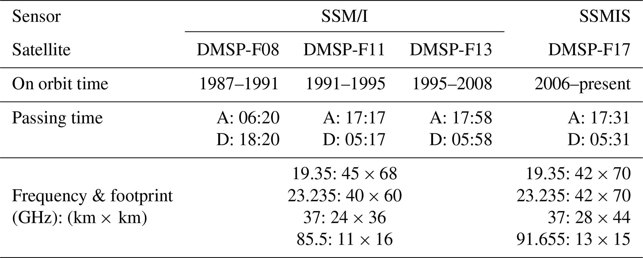
The series of Special Sensor Microwave/Imager (SSM/I) and Special Sensor Microwave Imager Sounder (SSMIS) instruments has provided continuous T_B measurements at 19.35, 23.235, 37, 85.5, and 91.655 GHz since July 1987. The data are available from the National Snow and Ice Center (https://daacdata.apps.nsidc.org/pub/DATASETS, last access: 21 March 2020). The SSM/I and SSMIS sensors are suitable for producing a consistent long-term snow depth dataset due to their similar configurations and intersensor calibrations (Armstrong et al., 1994). To avoid the influence of wet snow, only ascending (F08) and descending (F11, F13, and F17) overpass data were used (Table 1). In this study, the difference between 19.35 (36.5) GHz and 18.7 (37) GHz was ignored (hereafter referred to as 19 and 37 GHz, respectively).

Table 1 Summary of the main passive microwave remote sensing sensors.

(2) In situ measurements

The daily weather station data in China from 1987 to 2018 were provided by the National Meteorological Information Centre, China Meteorology Administration (CMA, http://data.cma.cn/en, last access: 21 January 2020). The geographical locations of the meteorological stations and the three stable snow cover areas are shown in Fig. 1. The recorded variables include the site name, observation time, geolocation (latitude and longitude), altitude (m), near-surface soil temperature (measured at a 5 cm depth, ^∘C), and snow depth (cm). The sites are not distributed homogeneously, and few are located in inaccessible regions with extreme climates and complex terrain conditions, e.g., the western part of the QTP (Fig. 1).

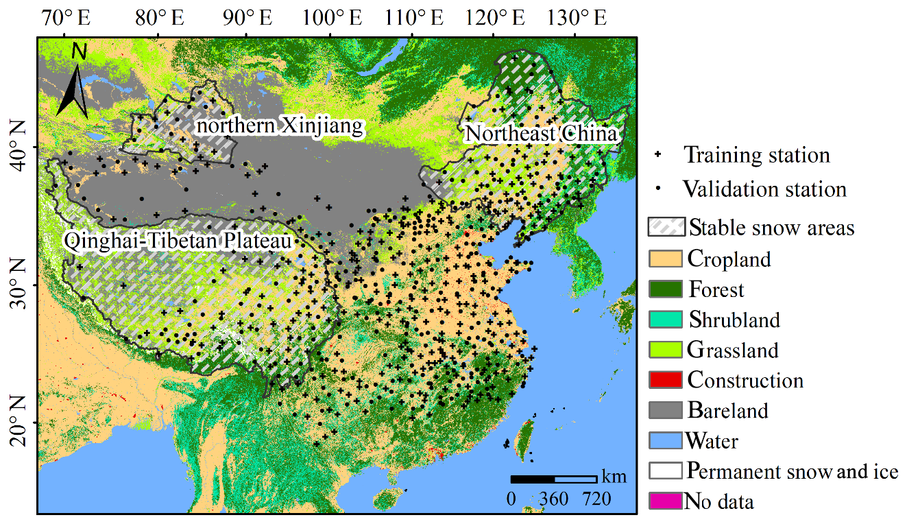
Figure 1 Spatial distribution of the weather stations and land cover types in the study area. There are three stable snow cover areas in China: northeast China (NEC), northern Xinjiang (XJ), and the Qinghai–Tibetan Plateau (QTP).

Quality control was conducted prior to using the data for developing and validating the retrieval algorithm. The first step was to select the records where the near-surface soil temperature was lower than 0 ^∘C. The second step was to remove the sites if the areal fraction of the open water exceeded 30 % within a satellite pixel. Finally, the 683 stations were randomly divided into two roughly equal-sized parts (Fig. 1). The snow depth observations from training stations (342 sites) together with satellite T_B and other auxiliary data can be used to train the RF model. The measurements from validation stations (341 sites), as independent data spatially, can be applied to validate the fitted RF algorithm. Figure 2 shows the histograms of snow depth observations from training and validation stations during the period 2012–2018. A total of about 90 % of the samples range from 1 to 25 cm. The maximum values of the snow depth extend to approximately 50 cm. However, the number of such cases is small and is therefore not evident in Fig. 2.

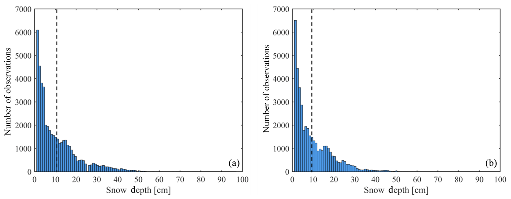
Figure 2 Histograms of snow depth observations from (a) training and (b) validation stations. The average values (black dashed lines) are equal to 10.5 and 9.8 cm, respectively.

(3) Land cover fraction

A 1 km land use and land cover (LULC) map derived from the 30 m Thematic Mapper (TM) imagery classification was provided by the Data Center for Resources and Environmental Sciences, Chinese Academy of Sciences (http://www.resdc.cn/, last access: 21 May 2019). The map was recalculated as the areal percentages of each land cover type in the 25 km grid cells. In this study, the fractions of grassland, bare land, cropland, forest, and shrubland were calculated as predictor variables of the RF model. To avoid the influence of water bodies and construction, the record was used only if the total fraction was greater than 60 %.

2.2 Methodology

2.2.1 Random forest

RF is an ensemble ML algorithm proposed by Breiman in 2001. It combines several randomized decision trees and aggregates their predictions by averaging in regression (Biau and Scornet, 2016). Generally, approximately two-thirds of the samples (in-bag samples) are used to train the trees and the remaining one-third (out-of-bag samples, OOB) are used to estimate how well the fitted RF algorithm performs. A few user-defined parameters are generally required to optimize the algorithm, such as the number of trees in the ensemble (ntree) and the number of random variables at each node (mtry). The ntree is set equal to 1000 in the present study since the gain in the predictive performance of the algorithm would be small with the addition of more trees (Probst and Boulesteix, 2018). The default value of mtry is determined by the number of input prediction variables, usually one-third for regression tasks (Biau and Scornet, 2016). The RF regression is insensitive to the quality of training samples and to overfitting due to the large number of decision trees produced by randomly selecting a subset of training samples and a subset of variables for splitting at each tree node (Maxwell et al., 2018). In addition, RF provides an assessment of the relative importance of predictor variables, which have proven to be useful for evaluating the relative contribution of input variables (Tyralis et al., 2019b). Furthermore, the RF model can be rapidly trained and is easy to use. In this paper, the randomForest R package (version 4.6–14) is used for regression (Liaw and Wiener, 2002; Breiman et al., 2018).

Table 2 A detailed description of the input predictor variables based on four selection rules of the training sample.

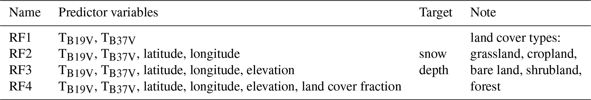
Table 3 Summary of three tests of the fitted RF algorithms in Table 2.

2.2.2 Feasibility study of the RF model

(1) Selection of predictor variables

The possible predictor variables used include geographic location (longitude, latitude), elevation, land cover fractions (grassland, cropland, bare land, shrubland, and forest), and multichannel brightness temperatures. All available channels on the SSM/I and SSMIS are listed in Table 1. The 23 GHz channel is sensitive to water vapor and not surface scattering, which introduces uncertainty to the estimation process (Ji et al., 2017). The 85 (91) GHz channel is seriously influenced by the atmosphere (Kelly, 2009; Xue and Froman, 2017). Typically, the lower frequency (19 GHz) is used to provide a background T_B against which the channels sensitive to higher-frequency (37 GHz) scattering are used to retrieve snow depth. The mixed-pixel problem is the dominant limitation on snow depth estimation accuracy (Derksen et al., 2005; Jiang et al., 2014; Roy et al., 2014; Cai et al., 2017; Li and Kelly, 2017). The satellite pixel usually covers several land cover types due to a coarse footprint. Thus, the land cover fractions were included as possible predictor variables. Previous studies have shown that geographic location and elevation indeed contribute to improving ML model performance (Bair et al., 2018; Qu et al., 2019).

To determine a suitable selection rule for training samples, we selected four combinations of predictor variables from training stations (Fig. 1) during the period 2012–2014 to train the RF algorithms. Table 2 presents a detailed description of the four selection rules of training samples. The correlations between the predictor variables and the variable importance metrics are shown in Fig. 3. The T_B measurements at horizontal polarization (H-pol) are highly correlated (correlations higher than 0.9) with observations at vertical polarization (V-pol). Moreover, according to their ranking of the predictor variables, the channels of V-pol are more relevant to the independent variable (snow depth) than are the H-pol channels. Therefore, the RF1 algorithm was trained with only two channels' T_B measurements at V-pol. The ranking of variables' importance in Fig. 3 indicates that the geographic location is more important than elevation to snow depth. Thus, the geographic location and elevation were included in the predictor variables of RF2 and RF3, respectively. Figure 3 also shows that the correlations between T_B and land cover fraction are relatively low. Thus, we will validate whether the inclusion of land cover fraction would increase the performance of the fitted RF4 algorithm.

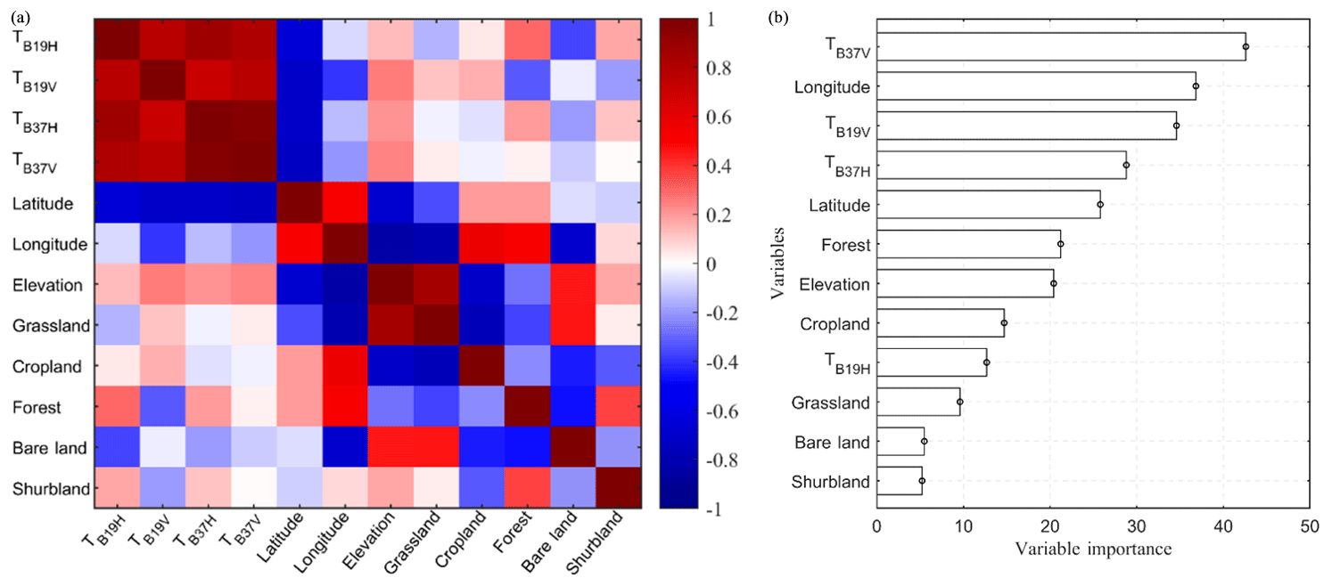
Figure 3 Correlations between the predictor variables (a) and the ranking of variable importance (b). The importance of variables, referred to as mean decrease accuracy (MDA) in the RF model, is obtained by averaging the difference in out-of-bag error estimation before and after the permutation over all trees. The larger the MDA, the greater the importance of the variable is.

(2) Training sample size

One of the advantages of the RF model is that it can effectively handle small sample sizes (Biau and Scornet et al., 2016). A test was conducted to demonstrate the insensitivity of the RF model to the training sample size. The input predictor variables include geographic location and T_B (Table 2, RF2). The flowchart of the test process is shown in Fig. 4. To ensure a sufficient number of samples, all station records (approximately 100 000 samples) from 1987 to 2006 were used to analyze the sensitivity of the RF model to the training sample size. A total of 5000 to 80 000 (with a step of 5000) samples selected randomly from data during the period 1987–2004 were used to respectively train the RF models, and a 2-year stand-alone dataset from 2005 to 2006 was applied to assess the performance of the trained models. We consider three evaluating indicators (the unbiased root-mean-square error (RMSE), bias, and correlation coefficient) to illustrate the sensitivity of the RF model to the training sample size.

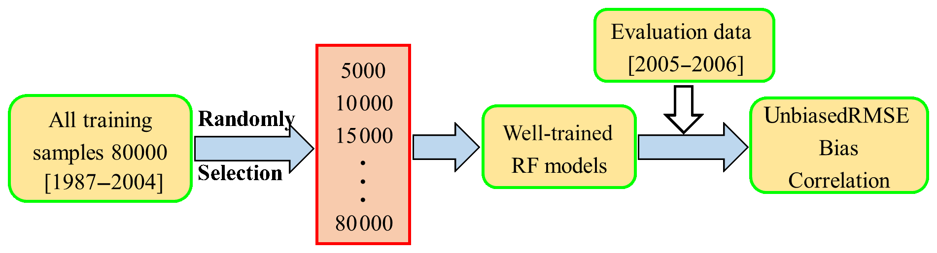
Figure 4 The test process flowchart for the sensitivity of the RF model to the training sample size.

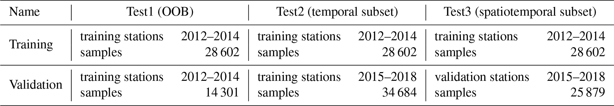
(3) Validation datasets of the fitted RF algorithms

We conducted three tests to verify the fitted RF algorithms (Table 3). The same training samples (same algorithms) were used for the three tests but with different validation datasets. In Test1, the validation data were from OOB samples. This preliminary assessment generally offers a simple way to adjust the parameters of the RF model. However, the OOB errors should be used with caution because its samples are not independent at temporal and spatial scales. In Test2, we applied independent reference data during the period 2015–2018 to assess the accuracy of the temporal prediction of fitted algorithms. Although this dataset is composed of observations from training stations in Fig. 1, it is temporally independent of the training samples (2012–2014). Generally, the RF model cannot extrapolate outside the training range (Hengl et al., 2018). Thus, in Test3, a spatially independent dataset from validation stations during the period 2015–2018 was used to assess the accuracy of spatiotemporal prediction. The unbiased RMSE, bias, and correlation coefficient are used for the assessment of the predictive performance of the fitted algorithms.

2.2.3 Validation of reconstructed snow depth product and trend analysis

The reconstructed long-term snow depth dataset was evaluated by the stand-alone ground truth measurements over the period 1987–2018 from the validation stations (Fig. 1). The reconstructed product was also compared with the static linear-fitting algorithm developed by fitting 19 and 37 GHz with the snow depth measurements with a constant empirical coefficient over China (Che et al., 2008). The daily snow depth data were obtained from the Environmental and Ecological Science Data Center for West China (http://data.casnw.net/portal/, last access: 21 March 2020) (hereafter WESTDC product). Then, the spatiotemporal patterns of snow depth were analyzed in northeast China (NEC), northern Xinjiang (XJ), and the QTP. The slope method (regression) was employed to analyze the snow depth variation trend at the temporal scale (Huang et al., 2019). To show the spatial distribution of snow depth variation, the Mann–Kendall test (significance levels of α=0.05) was used to analyze the trends of changes in China (Mann, 1945; Kendall, 1975; Milan and Slavisa, 2013). To ensure the presence of dry snow cover, the reconstruction periods are the main snow winter season (January, February, March, November, and December).

3 Results

3.1 Sensitivity to training sample size

The sensitivity of the RF model toward the training sample size was evaluated to confirm the appropriate number of training samples. Figure 5 displays the accuracy according to unbiased RMSE, bias, and correlation coefficient. These accuracy indexes show slight fluctuations when the number of training samples increases from 5000 to 80 000. Figure 5a shows that the unbiased RMSE ranges from 5.1 to 5.5 cm with increasing training samples. Figure 5c shows that the correlation coefficient is as high as 0.79 and becomes stable when the samples are up to 30 000. According to the sensitivity analysis, the number of training samples has less influence on the prediction accuracy of the RF model. This test is very helpful for us to determine the number of training samples because of the limited number of training samples over the period 2012–2014. We selected all available samples (28 602) from training stations (Fig. 1) during the period 2012–2014 to train the RF models in Table 2.

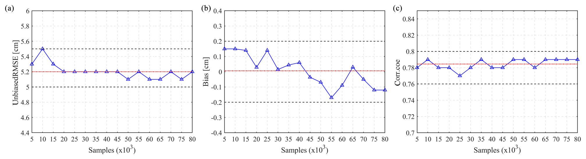
Figure 5 Trends of (a) unbiased RMSE, (b) bias, and (c) correlation coefficient with increasing training sample size.

3.2 Validation of the fitted RF algorithms

The fitted RF algorithms were evaluated by three validation datasets as shown in Table 3. The color–density scatterplots of the measured snow depth versus the retrieved snow depth are presented in Fig. 6. For all fitted RF algorithms (RF1, RF2, RF3, and RF4), notable differences in accuracy were revealed through the validation of three datasets (Table 4). Generally, the validation with OOB samples presented higher overall accuracy than the other two datasets. This result, however, does not demonstrate that the fitted RF algorithm performs well in snow depth estimation. The assessments in Test2 (temporal subset) and Test3 (spatiotemporal subset) demonstrate that the temporal prediction of the RF model outperforms the spatiotemporal prediction, with unbiased RMSEs of 4.4–5.4 cm and 7.2–7.9 cm, respectively.

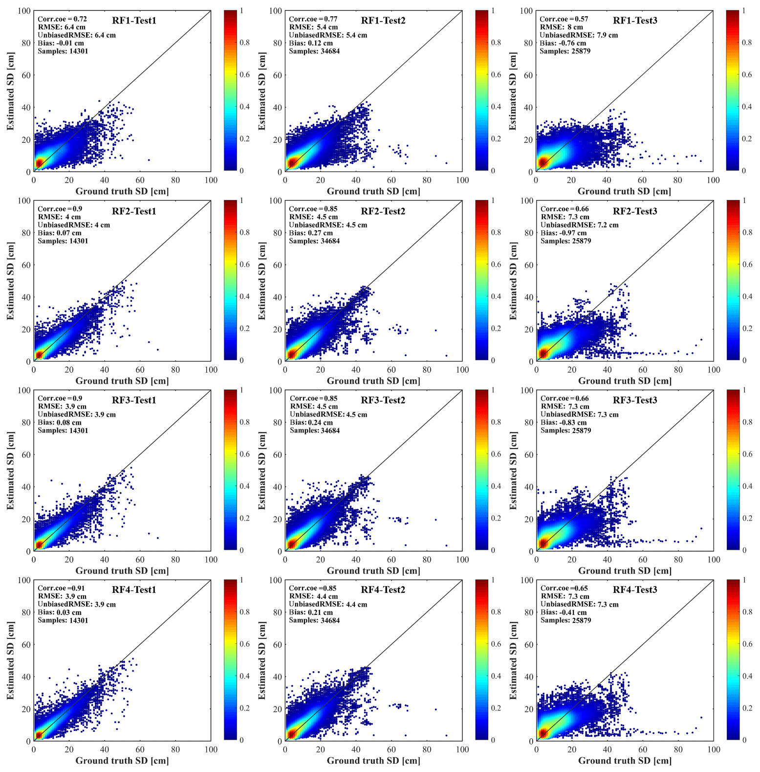
Figure 6 The color–density scatterplots of the estimated snow depth with four fitted RF algorithms and the ground truth snow depth. The four trained RF algorithms (RF1, RF2, RF3, RF4) were evaluated with three validation datasets (Test1, Test2, Test3).

Table 4 Accuracy of four snow-depth retrieval models with unbiased RMSE, bias and correlation coefficient.

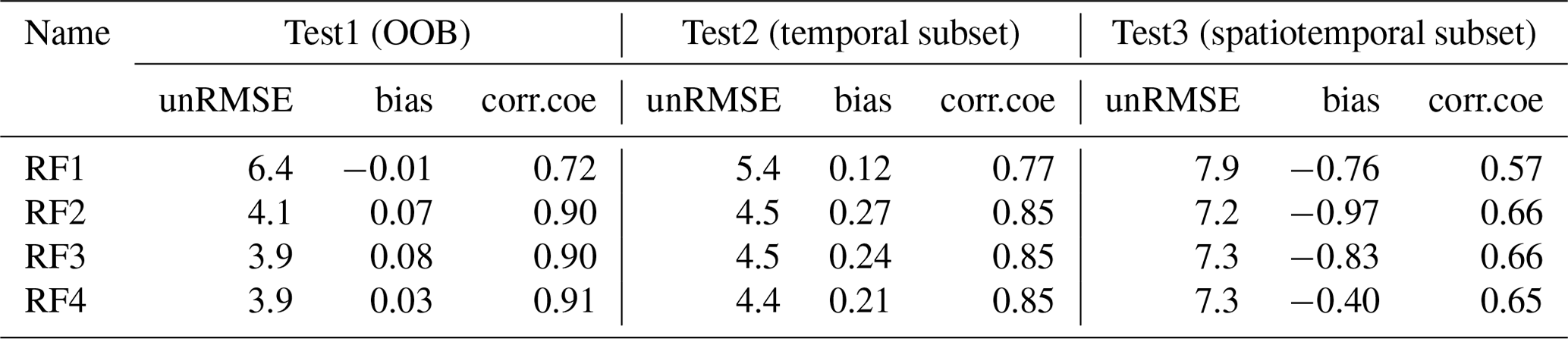
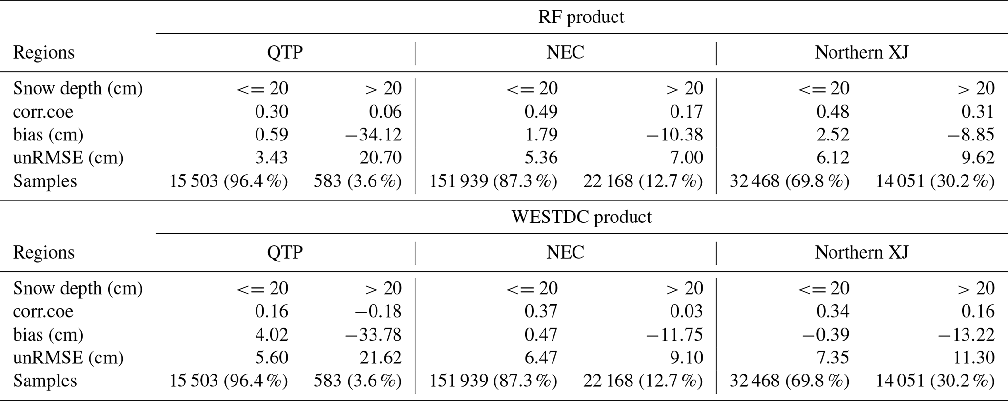
Table 5 Comparison between RF estimates and WESTDC product in three stable snow cover areas for deep (>20 cm) and shallow (≤20 cm) snow cover.

Comparing the validation results of RF1, RF2, RF3, and RF4, we find that the inclusion of auxiliary information indeed improved the performance of the fitted RF algorithms (Fig. 6). For Test1(OOB), the unbiased RMSE decreased from 6.4 to 3.9 cm with increasing predictor variables of auxiliary information, while the correlation coefficient increased from 0.72 to 0.90 (Table 4). For Test2 (temporal subset), the unbiased RMSE decreased from 5.4 to 4.4 cm and the correlation coefficient increased from 0.77 to 0.85 (Table 4). There was a slight improvement in spatiotemporal prediction when including the auxiliary information, with the unbiased RMSE ranging from 7.9 to 7.3 cm (Table 4).

3.3 Validation of the reconstructed snow depth product

According to the results in Fig. 6 and Table 4, there are no notable differences in accuracy among the RF2, RF3, and RF4 algorithms. In this study, we selected the RF2 algorithm to reconstruct a long-term snow depth dataset (1987 to 2018). We used the independent in situ measurements over the period 1987–2018 from validation stations (Fig. 1) to evaluate this product (hereafter RF product). Figure 7 shows the scatter diagrams of estimated vs. measured values for RF and WESTDC products. The overall accuracy of the RF product is higher than that of the WESTDC estimates, with unbiased RMSEs of 7.1 and 8.5 cm, respectively (Fig. 7a and b). The correlation coefficient is 0.65, which is larger than the WESTDC's coefficient of 0.49. Both products particularly underestimate snow depth when snowpack is thicker than 20 cm. The error bar shows that the WESTDC product tends to more seriously underestimate snow depth than do the RF estimates.

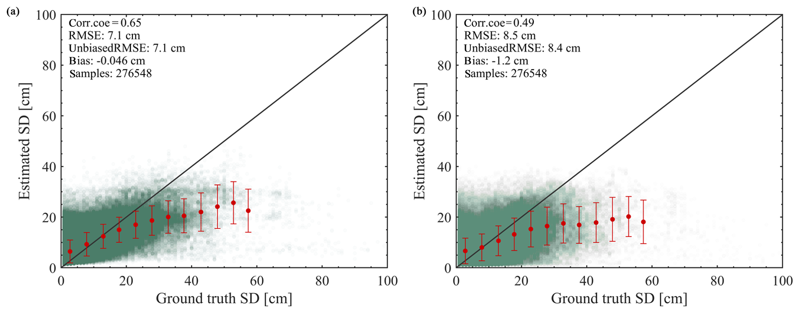
Figure 7 Scatterplots of the estimated snow depth and the ground truth observation for (a) RF and (b) WESTDC products.

To determine the interannual variability in the uncertainty, the time series of assessment indexes, including the unbiased RMSE, bias, and correlation coefficient, are shown in Fig. 8. The results show that the RF estimates outperform the WESTDC product with respect to unbiased RMSE and correlation coefficient from season to season. The bias also fluctuates from season to season, ranging from −8 to 3 cm (Fig. 8c). There is a slight overestimation during the period 1987–2000, whereas it presents a notable underestimation since 2006. Snow depth estimates with PMW data are usually challenged by the snow metamorphism (e.g., snow grain size). In particular, the large diurnal temperature range in the late snow season leads to a rapid snow grain growth (Dai et al., 2012). Figure 9 presents the monthly performances of both RF and WESTDC products. The RF estimates outperform the WESTDC product in terms of correlation, overall bias, and unbiased RMSE. WESTDC estimates tend to be underestimated in November, December, and March, while the RF product is superior to the WESTDC data. Due to the influence of the seasonal evolution of snowpack, the unbiased RMSEs of both products present increasing trends from November to March during the snow seasons. The correlation coefficient in January is the highest among snow season months, which is attributed to stable snow cover.

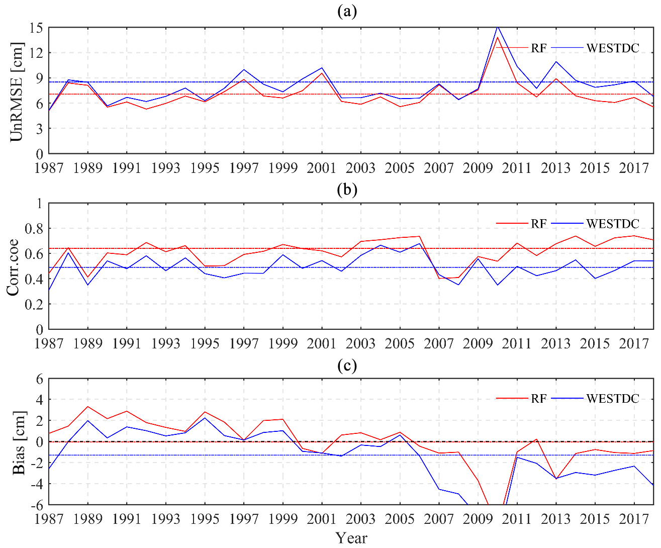
Figure 8 Time series of (a) unbiased RMSE (unRMSE), (b) correlation coefficient (corr.coe), and (c) bias for RF and WESTDC products. The colorful dashed lines represent mean values of assessment indexes.

The assessment of snow depth product was performed in three snow cover areas of China. As shown in Fig. 10a, the RF data are superior to the WESTDC estimates, with the unbiased RMSEs of 8.3, 6.8, and 8.8 cm in the QTP, NEC, and northern XJ for the RF product, respectively. Figure 10b shows a notable underestimation and overestimation for the WESTDC product in northern XJ and the QTP, respectively. For the RF product, the bias is close to zero and fluctuates across a relatively narrow range in the three snow cover areas.

Based on the results in Fig. 7, we selected 20 cm as a threshold to assess the performances in deep (>20 cm) and shallow (≤20 cm) snow cover. The percentage of shallow snow conditions to total samples was approximately 90 %. Table 5 displays the comparison between RF estimates and the WESTDC product in the three snow cover areas. The “Samples” row in Table 5 shows the number of samples and the corresponding percentage in each region. Both products present notable underestimation of deep snow cover, with biases of −34.1 and −33.8 cm on the QTP for the RF and WESTDC products, respectively. The biases are −10.4 and −8.9 cm for the RF product in NEC and northern XJ, respectively, whereas the same biases are −11.8 and −13.2 cm for the WESTDC data. Moreover, the correlation is very poor in deep snow cover, even negative (−0.18) in the QTP for the WESTDC product. For shallow snow cover, the RF product is superior to the WESTDC estimates in the QTP, with unbiased RMSEs of 3.4 cm (RF) and 5.6 cm (WESTDC). Furthermore, the WESTDC product presents overestimation in the QTP, with a bias of 4.0 cm that is much higher than the RF's bias of 0.6 cm. The unbiased RMSEs of the RF product are 5.4 and 6.1 cm in NEC and northern XJ for shallow snow cover, respectively, lower than the WESTDC's values of 6.5 and 7.4 cm. However, the RF product tends to overestimate snow depth relative to WESTDC estimates, with higher biases of 1.8 and 2.5 cm than WESTDC's 0.5 and −0.4 cm in NEC and northern XJ, respectively.

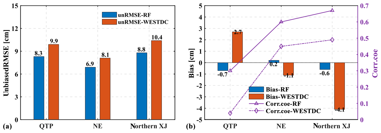
Figure 9 The validation of RF and WESTDC snow depth products in three stable snow cover areas over China with respect to (a) the unbiased RMSE, (b) bias, and correlation coefficient.

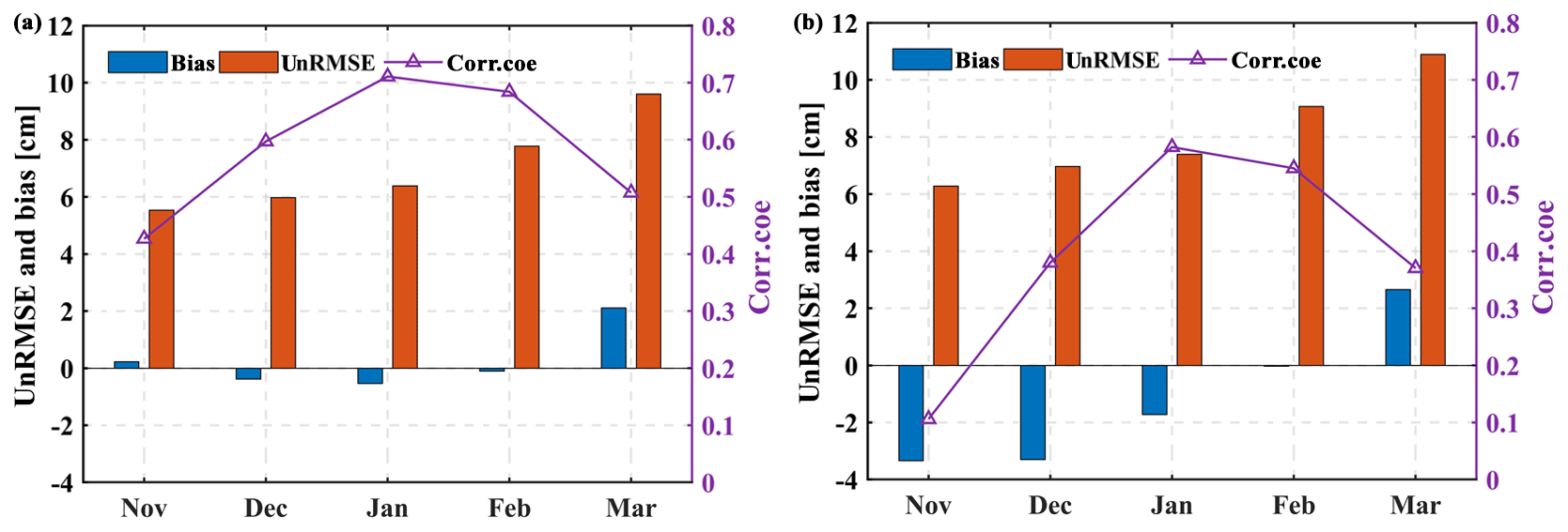
Figure 10 Monthly performances of (a) RF and (b) WESTDC snow depth products. Nov: November; Dec: December; Jan: January; Feb: February; Mar: March.

3.4 Spatial–temporal analysis of snow depth in three snow cover areas

The trend analysis of snow depth was conducted based on ground truth observations, the RF dataset, and the WESTDC product during the period 1987–2018. The time series of yearly mean snow depth in different regions over China is shown in Fig. 11. The red, green, and blue solid lines represent yearly mean snow depth in northern XJ, NEC, and the QTP, respectively. The black solid line displays the overall mean snow depth in China. Figure 11a shows that the ground truth snow depth in China presents a significant increasing trend from 1987 to 2018, with a correlation coefficient of 0.57. The trend in NEC is highly consistent with the overall trend over China, with a correlation coefficient of 0.64 (Fig. 11a). Although there are increasing trends in northern XJ and the QTP, the correlation coefficients are lower than 0.40, not significant (Fig. 11a). Figure 11b and c show the time series of yearly mean snow depth from the RF and WESTDC products, respectively. Neither of these values present significant trends. In the QTP, the WESTDC product presents a significant decreasing trend, with a correlation coefficient of −0.55 (Fig. 11c). Snow depth in northern XJ is the greatest among three snow cover areas, and snow cover in the QTP is very shallow, approximately 5 cm (Fig. 11a and b). With respect to magnitude and change trends, the ground truth observations and RF estimates in this study are consistent.

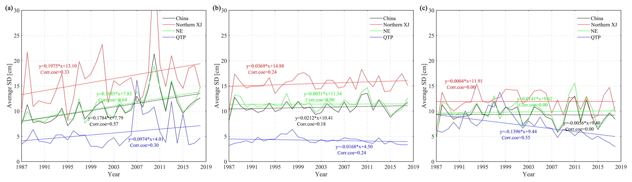
Figure 11 Trend analysis of snow depth based on (a) station observations, (b) RF estimates, and (c) WESTDC product in three stable snow cover areas of China. The correlation is statistically significant at the 0.05 level.

Figure 12 shows the spatial patterns of snow depth variation based on the RF and WESTDC products. Only the area with continuous snow depth measurements from 1987 to 2018 is shown in Fig. 12. The two products show similar patterns in most areas over China. There are notable trend differences between RF and WESTDC products in the northeast of the QTP and western NEC. The RF product presents an increasing trend in the northeast of the QTP, whereas a significant decreasing trend is presented for the WESTDC product (Fig. 12a and b). In western NEC, there is a significant increasing trend for the RF product but no significant trend for WESTDC data.

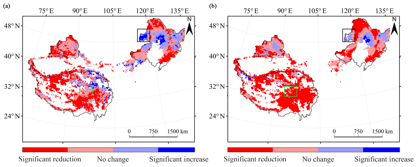
Figure 12 Trend analysis of snow depth during the period 1987–2018: (a) RF product; (b) WESTDC data. Light red and light blue represent no significant trend changes.

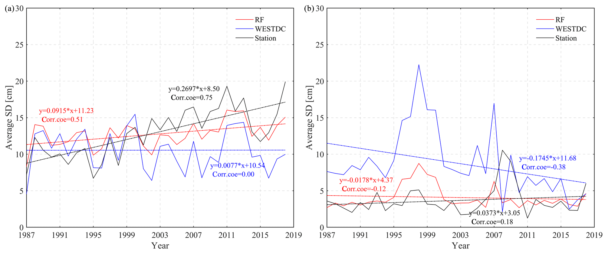
Figure 13 Comparison of changing trends of snow depth between RF estimates and the WESTDC product in specific areas of (a) NEC and (b) the QTP.

Based on the comparison of trends in Fig. 12 and available station observations in Fig. 1, we selected two specific areas (black and green grids in Fig. 12) to test the changing trend. Figure 13 shows the trends of snow depth based on the station observations (black solid line), RF estimates (red solid line), and WESTDC product (blue solid line). The ground truth snow depth presents a significant increasing trend in the specific area of NEC, with a high correlation coefficient of 0.75 (Fig. 13a). The RF product shows a significant increasing trend, which is consistent with the ground truth data (Figs. 12a and 13a). Figure 13b shows that the WESTDC product displays a decreasing trend in the selected area of the QTP, while station observations and RF estimates present no significant trends.

4 Discussion

4.1 Disadvantages of the RF model

The RF technique is already used to generate temporal and spatial predictions. Generally, the RF model cannot extrapolate outside the training range (Hengl et al., 2018). Figure 6 and Table 4 indicate that the spatial predictions of fitted RF algorithms are more biased than are the temporal predictions. Thus, the transferability of a fitted RF algorithm to other areas is in question. Several studies (Prasad et al., 2006; Hengl et al., 2017; Vaysse and Lagacherie, 2015; Nussbaum et al., 2018) have proven that RF is a promising technique for spatial prediction; however, these studies aim to obtain spatial predictions of elements of stationarity in the Earth system, e.g., soil types and soil properties.

The Earth system is interesting because it is nonstationary (especially concerning snow parameters). Generally, snow depth increases at the beginning of winter and then decreases in spring due to melting. Moreover, snow cover has different spatial patterns in various regions, such as generally deep snow in high-latitude and high-elevation areas. In China, there are five climatological snow classes according to the classification by Sturm et al. (1995). Each snow class is defined by an ensemble of snow stratigraphic characteristics, including snow density, grain size, and crystal morphology, which influences the snowpack's microwave signature (Sturm and Wagner, 2010). These dynamic properties of snow will lead to many cases in which the same satellite T_B corresponds to different snow depths, while the same snow depth is associated with various T_B observations, rendering the fitted RF algorithm suboptimal. Physical snow evolution models, e.g., the Snow Thermal Model (SNTHERM) (Jordan, 1991), SNOWPACK (Lehning et al., 2002a, b), and Crocus (Brun et al., 1989; Vionnet et al., 2012), can be used to simulate snow parameters (e.g., grain size, density) relatively accurately. Thus, integrating a priori knowledge of snowpack into ML techniques has the potential to overcome many limitations that have hindered a more widespread adoption of ML approaches.

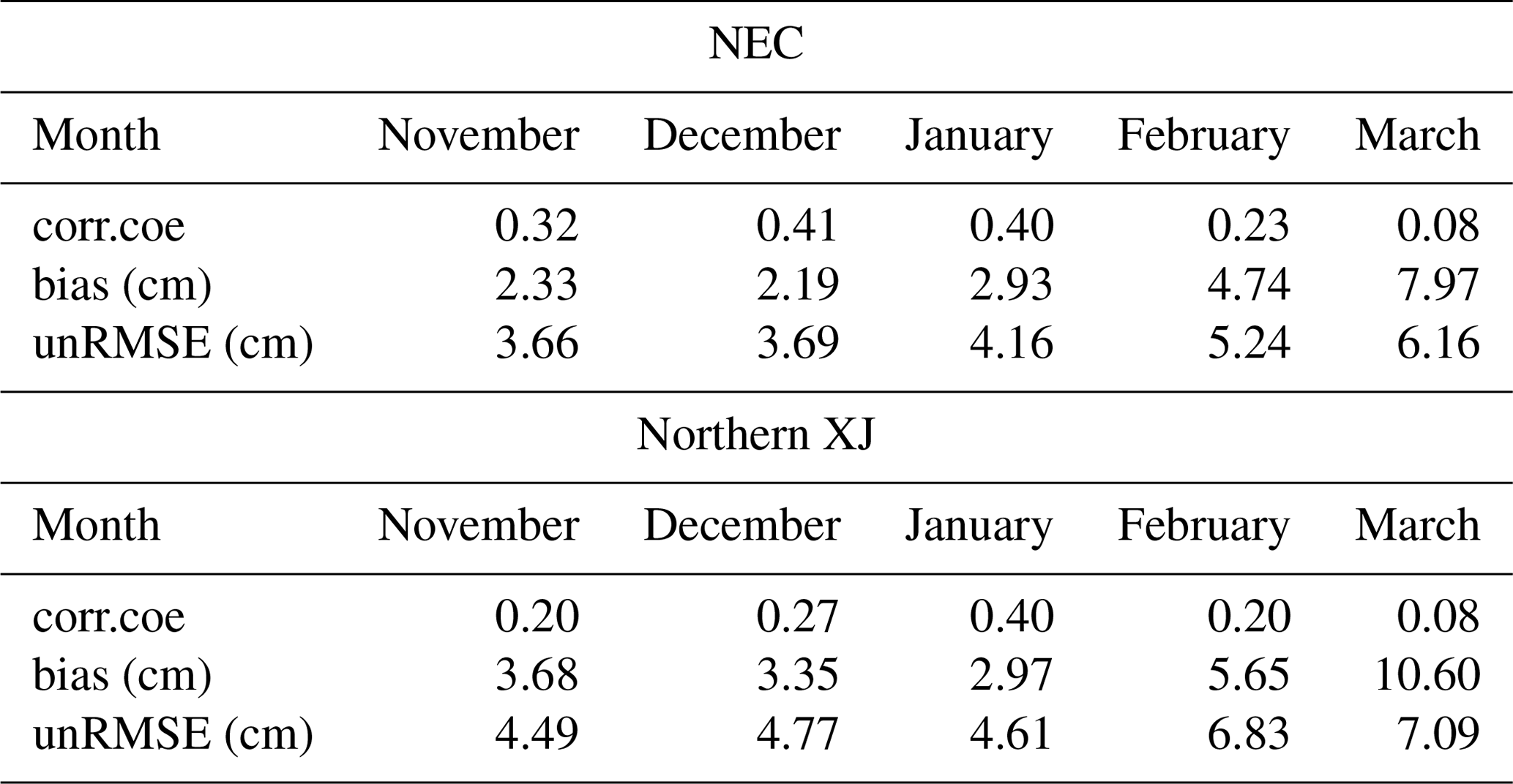
Table 6 Summary of monthly performances of the RF product in NEC and northern XJ.

4.2 Influence of predictor variables on the RF model

Figure 6 and Table 4 indicate that the inclusion of correlated predictor variables has a very slight influence in the predictive performance. Geographic location contributes to improving the RF model's temporal and spatiotemporal estimates, and the inclusion of both elevation and land cover fraction does not further improve the performance of the fitted models (Fig. 6). This is because elevation is highly correlated (correlations higher than 0.9) with geographic location (Fig. 3). Figure 3 also indicates that the correlation between longitude or elevation and land cover type (e.g., grassland, cropland, forest, and bare land) is significant. However, this correlation does not mean that the effects of elevation and land cover fraction on fitted RF model can be ignored. We tested the RF algorithms trained with T_B and elevation or land cover fraction data. The results (not shown here) indicate that these auxiliary data do improve the performance of the fitted algorithms. Strongly correlated variables have a very slight influence on the predictive performance of the RF model (Boulesteix et al., 2012). Therefore, in some cases, a few representative predictor variables should be selected.

4.3 Potential errors of the reconstructed snow depth

Figure 7 indicates that the RF model does not fully solve the overestimation and underestimation problems. For deep snow (>20 cm), the biases are up to −8.9 and −10.4 cm in NEC and northern XJ, respectively. Deep snow conditions account for approximately 10 % of all training samples (Fig. 2). The estimates for deep snow cover in the QTP exhibit a large bias of −34.1 cm. Figure 6 also illustrates that the fitted RF algorithms have no predictive ability for extremely deep snow conditions, especially in the QTP. We checked the training data and found that the extreme high snow depth data (>60 cm) occurred in the QTP. However, the number of such cases is very small. In addition, the station measurements are point values while the satellite grids have a spatial resolution of 25 km×25 km. Thus, the representativeness of these data is questionable. Snow depth estimation in the mountains remains a challenge (Lettenmaier et al., 2015; Dozier et al., 2016; Dahri et al., 2018). Numerous studies have been conducted on the snow cover over the QTP and have indicated that the snow cover in the Himalayas is higher than elsewhere, ranging from 80 % to 100 % during the winter (Basang et al., 2017; Hao et al., 2018). Additionally, Dai et al. (2018) showed that deep snow (greater than 20 cm) was mainly distributed in the Himalayas, Pamir, and southeastern mountains. Thus, the RF product produced in this paper has poor performance in the QTP for the deep snow cover.

Table 5 indicates that there is overestimation in NEC and northern XJ for shallow snow cover, which may be due to the following reasons. First, the PMW signals are insensitive to thin snow cover (<5 cm), especially for fresh snow with low snow density and snow grain size, which generally results in underestimation (Foster et al., 2005). In contrast, it tends to overestimate snow depth for shallow old snow in the late snow season due to the seasonal evolution of snowpack. For example, the large diurnal temperature range in the late snow season tends to subject the snowpack to frequent freeze–thaw cycles and leads to rapid snow grain (∼2 mm) and snow density (200–350 kg m⁻³) growth and consequently a high T_B difference (Meløysund et al., 2007; Durand et al., 2008; Yang et al., 2015; Dai et al., 2017). Thus, the overall bias and unbiased RMSE for shallow snowpacks (<10 cm) present increasing trends from November to March in NEC and northern XJ (Table 6). Second, frozen soil reduces the accuracy of estimates. Both snow and frozen ground are volume-scattering materials, and they have similar microwave radiation characteristics, making them difficult to distinguish. Third, a limiting factor in estimating snow depth for PMW remote sensing is the presence of liquid water. In this study, a snow cover detection method is used to filter out wet snow cover; however, there are still misclassification errors, especially at the end of the winter season (Grody and Basist, 1996; Liu et al., 2018a). In such cases, satellite observations are mainly associated with the emissions from the wet surface of the snowpack. Therefore, in wet snow conditions, snow depth retrieval is not possible (Derksen et al., 2010; Tedesco and Jeyaratnam, 2016).

5 Conclusions

The present study analyzed the application of the RF model to snow depth estimation at temporal and spatial scales. Temporally and spatially independent datasets were applied to verify the fitted RF algorithms. The results suggested that the accuracy of fitted RF algorithms was greatly influenced by auxiliary data, especially the geographic location. However, the inclusion of strongly correlated predictor variables (elevation and land cover fraction) did not further improve the RF estimates. Therefore, in some cases, a few representative predictor variables should be selected. Due to naive extrapolation outside the training range, the transferability of a fitted RF algorithm at the temporal scale was better than that in spatial terms, e.g., with unbiased RMSEs of 4.5 and 7.2 cm for the RF2 algorithm, respectively.

In this study, the fitted RF2 algorithm was used to retrieve a consistent 32-year daily snow depth dataset from 1987 to 2018. Then, an evaluation was carried out using independent reference data from the validation stations during the period 1987–2018. The overall unbiased RMSE and bias were 7.1 and −0.05 cm, respectively, outperforming the WESTDC product (8.4 and −1.20 cm). In the QTP, the unbiased RMSE and bias of RF estimates for shallow (≤20 cm) snow cover were 3.4 and 0.59 cm, respectively, much lower than WESTDC's 5.6 and 4.02 cm. In NEC and northern XJ, RF estimates were superior to the WESTDC product but still presented an underestimation for deep snow (>20 cm), with biases of −10.4 and −8.9 cm, respectively.

Three long-term (1987–2018) datasets, including ground truth observations, RF estimates, and the WESTDC product, were applied to analyze the trends of snow depth variation in China. The results suggested that there existed different trends among the three datasets. The overall trend of snow depth in China presented a significant increasing based on the ground truth observations, with a correlation coefficient of 0.57. Moreover, the trend in NEC was highly consistent with the overall trend in China, with a correlation coefficient of 0.64. Neither the WESTDC nor the RF product presented significant trends except in the QTP. The WESTDC product showed a significant decreasing trend in the QTP, with a correlation coefficient of −0.55, whereas there were no significant trends for ground truth observations and the RF product.

As discussed in Sect. 4, our reconstructed snow depth estimates are still challenged by several problems, e.g., underestimation for deep snow. Additional prior knowledge of snow cover, such as snow cover fraction, snow density, and snow grain size, is necessary to improve the RF model. Combining the physical snow evolution model (e.g., SNOWPACK) with the ML method will be the focus of future work. Furthermore, the mass balance approaches, e.g., the parallel energy balance model, will be used to improve the snow depth retrievals in high-altitude areas. In addition, although our results indicate that the RF method is a promising potential tool for snow depth estimation, there are a few pitfalls such as the risk of naive extrapolation and poor transferability in spatial terms limiting its application in spatiotemporal dynamics. It is in addressing these shortcomings that the techniques of deep learning promise breakthroughs. We are attempting to operate the deep neural networks (DNNs) model to overcome the limitations of traditional ML approaches.