the Creative Commons Attribution 4.0 License.
the Creative Commons Attribution 4.0 License.
 | 26 May 2020
Combining TerraSAR-X and time-lapse photography for seasonal sea ice monitoring: the case of Deception Bay, Nunavik
Sophie Dufour-Beauséjour
Anna Wendleder
Yves Gauthier
Monique Bernier
Jimmy Poulin
Véronique Gilbert
Juupi Tuniq
Amélie Rouleau
Achim Roth
This article presents a case study for the combined use of TerraSAR-X and time-lapse photography time series in order to monitor seasonal sea ice processes in Nunavik's Deception Bay. This area is at the confluence of land use by local Inuit, ice-breaking transport by the mining industry, and climate change. Indeed, Inuit have reported greater interannual variability in seasonal sea ice conditions, including later freeze-up and earlier breakup. Time series covering 2015 to 2018 were acquired for each data source: TerraSAR-X images were acquired every 11 d, and photographs were acquired hourly during the day. We used the combination of the two time series to document spatiotemporal aspects of freeze-up and breakup processes. We also report new X-band backscattering values over newly formed sea ice types. The TerraSAR-X time series further show potential for melt and pond onset.
- Article
(15353 KB) - Full-text XML
-
Supplement
(10977 KB) - BibTeX
- EndNote


1.1 Context
Salluimiut (people of Salluit, Nunavik, in Canada) have reported changes in their environment, including less snow in the winter, which affects their activities on the land in Deception Bay (Tuniq et al., 2017). This area is prized by local Inuit for fishing as well as seal and caribou hunting (Petit et al., 2011). People from the neighboring community of Kangiqsujuaq have reported warmer and longer fall seasons, later freeze-up (Nickels et al., 2005), and less snow and earlier sea ice breakup in spring (Cuerrier et al., 2015). Seasonal sea ice conditions in Deception Bay will continue to evolve: climate projections for the region include shorter snow cover periods and warmer annual average temperature in 2040–2064 (Mailhot and Chaumont, 2017). Further, two nickel mines have marine infrastructure in Deception Bay. Their icebreakers transit in the bay from 1 June to mid-March, avoiding the seal reproduction period (GENIVAR, 2012). From January to March, Raglan Mine's MV Arctic performs on average two round trips (Mussells et al., 2017).
Raglan Mine initiated this project in response to local concerns about sea ice conditions in Deception Bay. The Northern Villages of Salluit and Kangiqsujuaq and both communities' landholding corporations gave their approval for this project, including associated activities and instrumentation in Deception Bay. The Avataq Cultural Institute was consulted to ensure the project did not encroach on archeological sites important to Inuit. Finally, the Nunavik Marine Region Impact Review Board gave permission for the deployment of underwater sonars in Deception Bay (sonar data not presented in this article). Local sea ice monitoring is relevant in light of local community members' reliance on the fjord's rich ecosystem for subsistence, as well as for shipping-related operations by the mines. More generally, this case study stands out due to the length of the time series reported, and it may be useful to those wishing to monitor seasonal processes in remote areas or interested in sea ice processes.
1.2 Monitoring sea ice seasonal processes
First-year sea ice processes include, among others, formation through freeze-up, transformation of the snow and ice covers over the winter and spring, and eventual breakup. These processes may unfold differently from year to year due to meteorological conditions, over a period of time which may vary from a single day to weeks. They may be driven by environmental factors such as air temperature, wind, currents, and precipitation, to name several. The sequence of events may vary from one area to another, influenced by geomorphological features like shallows or deep water pockets, islands, and rivers. To capture the spatiotemporal nature of these processes, their observation should therefore integrate both spatial coverage and frequent observations. The combined use of radar remote sensing and time-lapse photography meets these requirements.
Synthetic aperture radar (SAR) sensors are uniquely qualified for winter applications in the polar regions: they can acquire images in the dark and through clouds. Modern options combine wide coverage and high spatial resolution with a revisit period as short as 11 d, in the case of TerraSAR-X (X band, 9.65 GHz). X-band SAR has been shown to be a useful complement to the conventional C band when it comes to first-year sea ice: it was used to identify types of new ice (Johansson et al., 2017), particularly thin ice like nilas and gray ice (Matsuoka et al., 2001). The X band is also reputed to be more sensitive to the snow cover and freeze–thaw processes than the C band (Eriksson et al., 2010). Although the literature on X-band backscattering from first-year sea ice is sparse when compared to the C band – two notable exceptions being Onstott (1992) and Nakamura et al. (2005) – several recent publications are bridging this gap. They include observations over new ice and nilas (Johansson et al., 2017; 2018) and white ice (Fors et al., 2016), as well as over first-year sea ice during the spring (Nandan et al., 2016, 2017; Paul et al., 2015). Recent studies have taken advantage of TerraSAR-X's frequent revisits to successfully document spatially extensive processes such as seasonal snow cover extent and snowmelt (Sobiech et al., 2012; Stettner et al., 2018), as well as glacier calving front monitoring (Zhang et al., 2019). In the C band, a substantial ERS-1 and RADARSAT-1 (C band, 5.405 GHz) time series spanning 8 years was aggregated to study the springtime backscattering signature of snowmelt processes on first-year sea ice (Yackel et al., 2007).
Time-lapse photography is well suited for long-term monitoring applications related to the cryosphere: the systems can be installed in remote locations and record data as often as hourly, for prolonged periods of time. Such time series have been used to track daily-to-seasonal variations in the extent of the sea ice and ice melange in front of a retreating glacier (Cassotto et al., 2015), to document glacier mass loss (Chauché et al., 2014) and albedo (Dumont et al., 2011), and to observe sea ice concentration in the Beaufort Sea (Wobus et al., 2011). Time-lapse photography has also been used to document snow accumulation and accretion processes on mountain slopes (Vogel et al., 2012), snow cover extent in the tundra (Kępski et al., 2017) and in forests (Arslan et al., 2017), and snowmelt (Farinotti et al., 2010; Ide and Oguma, 2013; Peltoniemi et al., 2018; Revuelto et al., 2016). Bongio et al. (2019) successfully automated snow thickness measurements using time-lapse photography and measurement stakes in forestrial and alpine regions. Meteorological information may be derived from the photographs, for instance precipitation type or wind conditions (Christiansen, 2001; Liu et al., 2015; Smith et al., 2003). Finally, Herdes et al. (2012) used subdaily time-lapse photography time series to validate and complement the visual interpretation of weekly RADARSAT-1 (C band) time series in the context of iceberg plumes and coincident sea ice conditions.
1.3 Objectives
This article explores the use of combined TerraSAR-X and time-lapse photography time series to monitor seasonal sea ice processes and the potential of time-lapse photography to support TerraSAR-X interpretation. We performed this case study over 3 years in Nunavik's Deception Bay. A complementary objective is to describe the processes through an interannual comparison.
Deception Bay (62∘09′ N, 74∘40′ W) is located on the northern edge of Nunavik, the Inuit Nunangat territory overlapping the Canadian province of Quebec north of the 55th parallel. This fjord of the Ungava Peninsula is roughly 20 km long and nested in hills peaking at 580 m in altitude (GENIVAR, 2012). Water depth in the bay (Fig. 1) reaches 80 m in the deepest section located between the marine infrastructure and Moosehead Island. Deception Bay is accessible from Hudson Strait by boat during the ice-free season or by icebreaker. It is also accessible in winter and spring by snowmobile from overland trails. The closest communities are Salluit (50 km west) and Kangiqsujuaq (200 km southeast). The study area corresponds to a 9 km long section of the bay, centered on the marine infrastructures (see Fig. 2).

Figure 1Elevation and bathymetry map of Deception Bay. Inset: Inuit Nunangat, with Nunavik in green. Marine infrastructures are identified with anchor markers.
The Canadian Ice Service, in its Climatic Ice Atlas 1981–2010, estimates freeze-up and breakup in the bay to occur around the first week of December and the first week of July, respectively (Fequet et al., 2011). Landfast sea ice typically extends to the mouth of the bay, where it is stabilized by Neptune Island. Point thickness measurements performed in Deception Bay for the Ice Monitoring project in January–February and April–May 2016, 2017, and 2018 (Gauthier et al., 2018) ranged from 0 to 55 cm for the snow cover and from 52 to 165 cm for the ice cover. Deception River is the largest river flowing into the bay, and its flow is greatest at the end of spring in June and July because of snowmelt; its flow is almost zero during the winter (GENIVAR, 2012). Water salinity in the bay ranges from 29 to 33 psu (GENIVAR, 2012).
In addition to TerraSAR-X and time-lapse photography data, which is described in this section, air temperature data were also considered. The nearest meteorological station is located 50 km west of the study area, at Salluit Airport, and partial air temperature measurements are acquired in the bay by time-lapse cameras. These two data sources are presented and compared in the Supplement, under “Air temperature in Deception Bay”. Data from Salluit Airport is presented in the Results section as either monthly mean air temperature or monthly cumulative freezing and thawing degree days (see Figs. S9 and S10 in the Supplement).

Figure 2Map of TerraSAR-X image subset, time-lapse camera locations, and Panasonic fields of view.
3.1 TerraSAR-X
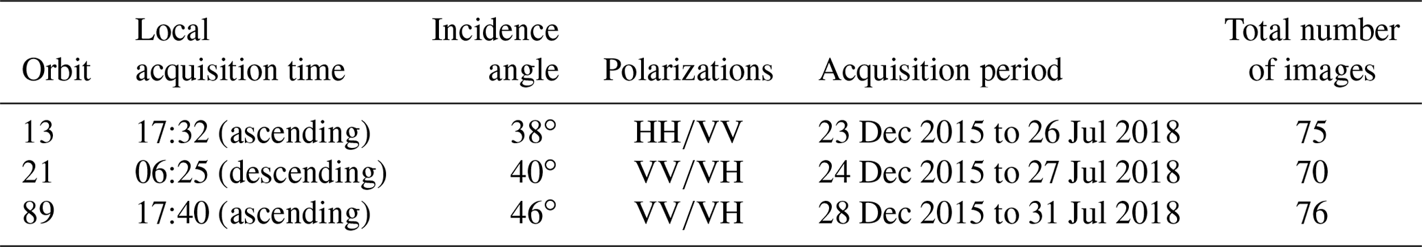
TerraSAR-X acquired StripMap dual co- and cross-polarization single look complex (SLC) images over Deception Bay from December 2015 to July 2018, spanning three winter seasons. This X-band satellite – and its counterpart TanDEM-X – operate at a central frequency of 9.65 GHz (3.11 cm wavelength), with a repeat period of 11 d. Three orbits overpass the study area (13, 21, 89); orbits 21 and 89 are respectively 1 and 5 d later than orbit 13. Each orbit yields a time series of images with identical acquisition parameters (see Table 1). Their incidence angles range from 38 to 46∘, in either ascending or descending passes, and they all include a VV polarization. The scene size before subsetting to the study area was 15 by 50 km, with a spatial resolution of 0.9 and 2.5 m, respectively, for range and azimuth directions (Eineder et al., 2008). Figure 2 shows the extent of the subimages, which cover a 9 km long section of the bay.
Table 1Characteristics of TerraSAR-X acquisitions for the study.
3.2 Time-lapse photography
A pan–tilt–zoom Panasonic WV-SW598 camera was installed on the southwest shore of Deception Bay (Fig. 2) on 11 September 2015. Operating in time-lapse mode, the camera takes a photograph every 15 min during the day (from 06:00 to 18:00 local time), rotating through four preset views (Fig. 2). The photographs have an effective pixel count of 2.4 MP, and a 90x zoom is available when setting the views or taking remote control of the camera. The camera can operate at temperatures between −50 and 55 ∘C and is installed at a height of 1.8 m. The selected site is accessible by foot from Raglan's marine infrastructure, located on a high point which offers a good view of the study area. Photographs are automatically transferred through Raglan's network to a database hosted by Institut national de la recherche scientifique (INRS). There are roughly 1400 photographs per month, for a total of almost 17 000 per year, all available to the general public on http://caiman.ete.inrs.ca (last access: 15 May 2020; Bernier et al., 2017).
We chose three general sea ice processes for spatiotemporal monitoring: freeze-up, wintering, and breakup. The wintering process is defined as a general term which may include winter sea ice processes such as ice desalination and snow reorganization. Specific elements characterizing each process were identified and observed through TerraSAR-X or time-lapse photography indicators. For example, the dates on which freeze-up begins and ends are respectively indicated by the first day where sections of the wintering ice cover are observed on the water and the first day where the wintering ice cover is complete and stable. Section 4.1 and 4.2 describe the process element indicators and how they are observed or measured from each data source. Section 4.3 details how we compared the photographs with coincident satellite images and identified their features, which serves to evaluate the potential of time-lapse photography to enhance TerraSAR-X image interpretation.
4.1 TerraSAR-X image processing and temporal interpretation
The TerraSAR-X images were used to document both the spatial and temporal aspects of the freeze-up, wintering, and breakup processes. Before being interpreted, the images were first processed at the DLR (German Aerospace Center), using the Multi-SAR-System. This workflow starts with a conversion from the digital number to radar brightness (sigma-naught), followed by multilooking to produce square pixels and increase the radiometric quality (number of looks), orthorectification so all the images from all orbits could be overlaid, and image enhancement to reduce the speckle inherent to SAR images (Schmitt et al., 2015). The Multi-SAR-System is described in detail in Bertram et al. (2016). The output images have a geometric resolution of 2.5 m pixels with a radiometric resolution of 1.6 looks. The TerraSAR-X noise floor for the three orbits ranges between −23 and −24.5 dB, the difference between maximum and minimum incidence angle within an image ranges from 1.4 to 1.0∘, and the radiometric accuracy is 0.6 dB (Eineder et al., 2008).
Median backscattering was computed for each subimage and plotted as a function of time for a given year. A total of 32 areas of interest (AOIs) were distributed over the study area, roughly 120 m by 100 m and containing between 2016 pixels and 2064 pixels each. Their locations were chosen to avoid the shore, man-made structures like docks, and broken ice left in the wake of icebreakers (Fig. 3). The median backscattering was computed over each AOI and then over all AOIs for a given subimage, yielding a single median value per subimage. This step was performed using Python (Dufour-Beauséjour, 2019).

Figure 3TerraSAR-X VV subimage of Deception Bay on 24 December 2015 in orbit 21 and AOIs used to compute statistics (yellow). The image is grayscaled from −19 to −5 dB.
Recurring seasonal features in all X-band VV median backscattering time series acquired during this study include two peaks separated by a monotone period. From this, four indicators were derived: the post-freeze-up peak (I), the beginning (II) and end (III) of the monotone period, and the spring peak (IV). Figure 4 shows examples for two different years and orbits, chosen for their clarity. Speaking in terms of the data time series, peak location is defined as the location of its maximum and estimated as sitting between the left- and right-hand neighbors of the highest data point. The beginning (end) of the monotone period is estimated as sitting between the first (last) monotone data point and its left-hand (right-hand) neighbor. Figure 4 shows an example of estimated ranges for each indicator, using two orbits and years chosen for their clarity. These ranges were identified manually and are presented for all orbits and years in Figs. S1–S3. The estimated range for a given indicator and year was further reduced by combining all available orbits (Fig. S1–S3). Finally, the winter trend was computed from a linear regression fit on the data in the monotone period, as shown in Fig. S4.
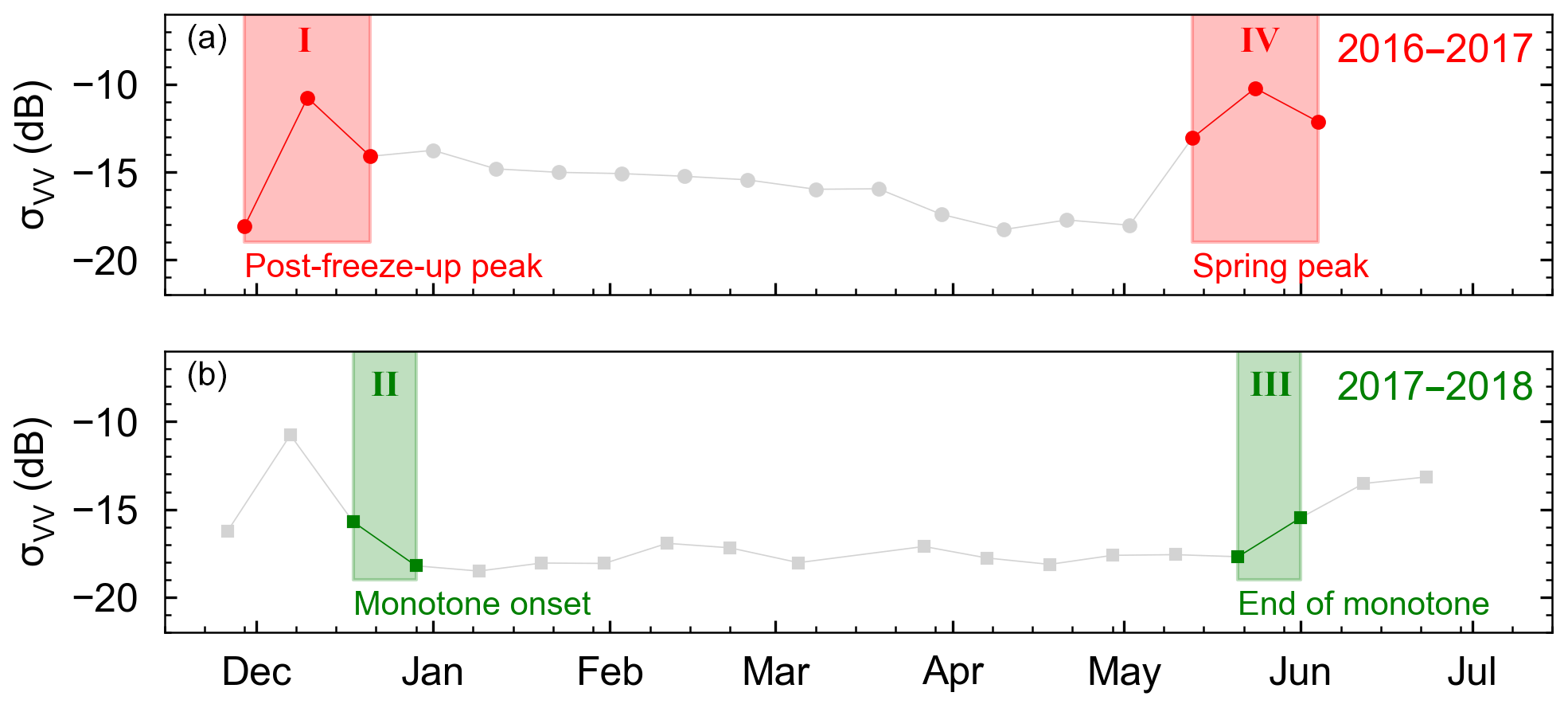
Figure 4Examples of change detection in TerraSAR-X VV median backscattering. Peak detection for orbit 21 in 2016–2017 (a), and inflexion detection for orbit 13 in 2017–2018 (b). Derived indicators are the post-freeze-up peak (I), the beginning (II) and end (III) of the monotone period, and the spring peak (IV).
4.2 Photograph interpretation
The photographs were interpreted to document both the temporal and spatial aspects of freeze-up and breakup processes. The freeze-up process includes the formation of various ice types in the study area up to their eventual consolidation into a continuous ice cover which stays in place for the whole winter. The breakup process includes the degradation and dislocation of the ice cover up to the total absence of ice.
During the freeze-up process, ice types were identified following WMO nomenclature as either grease ice (a soupy and matt layer of coagulated crystals), shuga (an accumulation of spongy white lumps a few centimeters across), nilas (a thin crust of matt ice which may raft in interlocking fingers), ice rind (a brittle and shiny crust of ice formed on a quiet surface, easily breaking into pieces), and pancake ice (pieces of ice up to 3 m in diameter which may be formed from the preceding types of ice and rapidly cover large expanses) (descriptions from WMO, 2014).
Consolidation of the ice cover was documented based on the persistence of features over time and their lateral movement. The date on which the freeze-up process was completed, called “the freeze-up date”, was also used as an indicator. For the breakup process, ice cover dislocation was documented based on the occurrence of open water. Ice cover degradation was documented based on its color and texture, as well as the occurrence of flooding. The date on which the breakup process was completed, called “the breakup date”, was also used as an indicator. Photograph sequences showing the freeze-up and breakup processes for each season are presented in the Video supplement (Movies S1–S6).
Figure 5 shows two examples of photograph interpretation. At the top, the 2016 breakup process unfolds: snow and ice covers degradation can be seen through changes in color and texture. At the bottom, the 2016 freeze-up process comes to an end on 29 November, where nilas patches on the water consolidate into a continuous ice cover whose features are immobile.
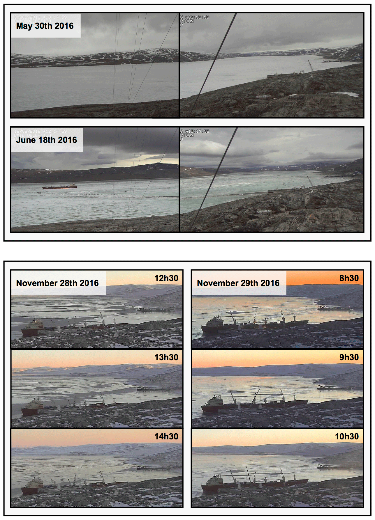
Figure 5Time-lapse photography during the 2016 breakup process (top) and the 2016 freeze-up process (bottom).
4.3 TerraSAR-X spatial interpretation using photography
TerraSAR-X images were interpreted using coincident photographs taken from the shore. Observed features include open-water areas or leads and different ice types. Figure 6 shows two examples. At the top, nilas, pancake ice and grease ice are observed on the photographs during the 2017 freeze-up process and then identified on a coincident TerraSAR-X image acquired on 26 November. At the bottom, ice cover dislocation is observed on photographs during the 2018 breakup process; leads and open areas are identified on the coincident 28 June image.
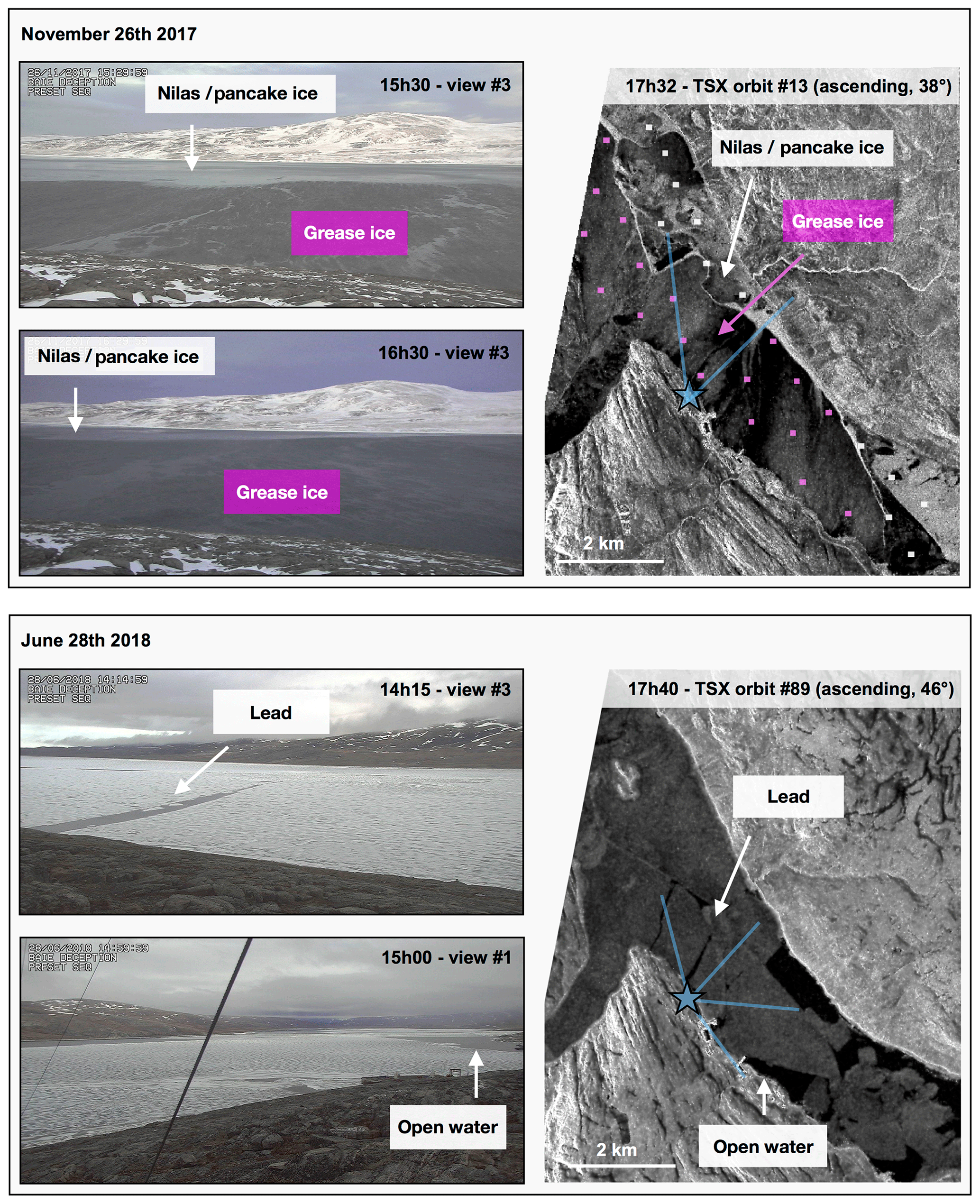
Figure 6Coincident time-lapse photography and TerraSAR-X images during the 2017 freeze-up process (top) and the 2018 breakup process (bottom). On the images, camera location and fields of view are identified in blue. Top: TerraSAR-X VV image from orbit 13. AOIs are color coded according to the identified ice type, prior to backscattering signature extraction. Bottom: TerraSAR-X VV image from orbit 89. Both images are grayscaled from −19 to −5 dB.
Results from the methods described above are spatiotemporal descriptions of sea ice seasonal processes, organized here following the seasons (freeze-up, wintering, and spring). Results from different sources and methods are presented together to facilitate interpretation.
5.1 Freeze-up
In the following description of processes for each year, we refer to zones represented in Fig. 7. No icebreaker transits occurred during the freeze-up process for the 3 years of this study. The freeze-up date is the first day featuring a consolidated ice cover which remains in place for the whole winter.
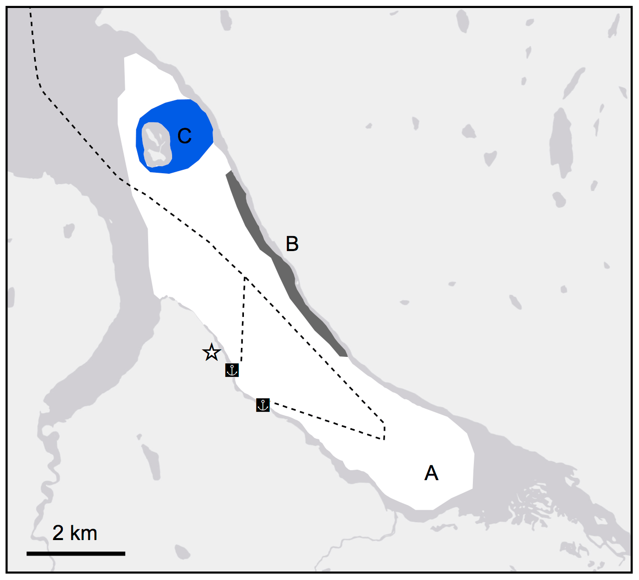
Figure 7Zones relevant for describing the spatial aspects of the freeze-up process in Deception Bay, and ship routes for the MV Arctic and MV Nunavik (dashed line). Camera location is indicated with a star.
In 2015, freeze-up was preceded by days featuring fog and open water, as well as grease ice and shuga. On 10 November, landfast ice appeared along the northeastern shore (zone B) and grew thermally, progressively extending to cover the whole study area (zone A) by 11 November 2015. In 2016, the days before freeze-up featured grease ice and open water, as well as the accumulation of pancake ice over the shallows near Moosehead Island (zone C). After the formation of nilas and various new ice types on 27 November, zone A was covered by mirror-like patches of nilas and ice rind on 28 November. Their lateral movement is illustrated in Fig. 5. The next morning, overlapping patches of nilas covered the study area. No lateral movement of the ice was observed on 29 November. Freeze-up was therefore completed on 29 November 2016. In 2017, a similar series of events was observed. Freeze-up was alternatively preceded by days of open water and days where the water was covered in grease ice or nilas, and pancake ice accumulated in zone C. On 27 November, zone A was covered with mirror-like nilas or ice rind. This ice was rearranged during the night into an ice cover which showed no further substantial lateral movement. Observed features shifted slightly southeast in the night between 29 and 30 November. Despite these minor tidal movements, we identify freeze-up as having occurred on 28 November 2017.
Following ice type identification from photographs, the X-band backscattering signature of newly formed ice types was extracted during the 2016 and 2017 freeze-up processes. An example of TerraSAR-X image interpretation from coincident photographs is shown in Fig. 6, where grease ice was observed as well as a mix of nilas and pancake ice. Figure 8 shows median VV backscattering values for AOIs over grease ice, nilas, pancake ice, and a mixture of the two. In the days following the 2016 and 2017 freeze-up dates, the young ice cover presented systematically higher backscattering than during the rest of the winter. Identification of a specific ice type was impossible from time-lapse photography, however, since young ice is characterized by its thickness (WMO, 2014). Figure 8 also shows median VV backscattering for AOIs over this unidentified young ice. Results are presented for different acquisition geometries and incidence angles (details in figure caption). The images associated with each box in Fig. 8 are reproduced in the Supplement (Fig. S5–S6) along with the color-coded AOIs used for each ice type.

Figure 8TerraSAR-X median VV backscattering values observed over AOIs of ice types identified from time-lapse photography in 2016 and 2017. The number of median values used (n) is written above each box. Outliers are plotted as empty white circles. (a) Grease ice (pink) was observed on the orbit 13 image from 26 November 2017. Nilas (dark purple) was observed on 28 and 29 November 2016 in orbits 13 and 21, respectively. A mix of nilas and pancake ice (white) was observed on 26 November 2017 in orbit 13. Pancake ice (yellow) was observed on 28 and 29 November 2016 in orbits 13 and 21. (b) Unidentified young ice (gray) was observed on 9 and 10 December 2016 in orbits 13 and 21, as well as on 1, 7 and 8 December 2017 in orbits 89, 13, and 21. The number of days since the freeze-up date (t) is written below each box.
Figure 9 shows the temporal evolution of the median VV backscattering during the freeze-up processes, as well as indicators derived from time-lapse photography and TerraSAR-X: the freeze-up date, the freeze-up peak (I), and the beginning of monotone backscattering (II). No TerraSAR-X data are available during the freeze-up in 2015. The daily event sequences (Tables S1–S3), as well as videos assembled from time-lapse photography (Movies S1–S3) and TerraSAR-X (Movies S7–S9), are available in the Supplement and Video supplement. Year 2015 saw an earlier freeze-up than the other years by 18 and 17 d (2017 and 2018). Mean temperatures measured over the years at Salluit Airport for October ranged from −3 ∘C in 2017 to −5 ∘C in 2015 and from −8 ∘C in 2016 to −11 ∘C in 2015 for November (see Fig. S9).
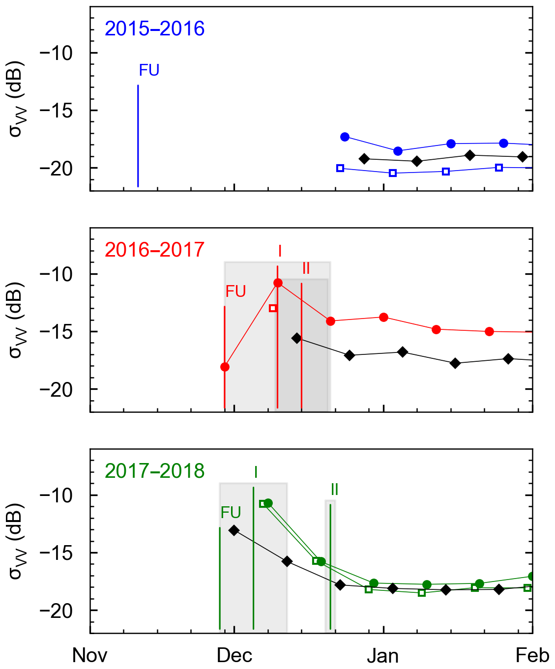
Figure 9TerraSAR-X median VV backscattering is plotted versus time for each year (color coded). Three orbits are shown for orbits 13 (empty square), 21 (circle), and 89 (black diamond). The freeze-up date (FU, from time-lapse photography), the post-freeze-up peak (I, from TerraSAR-X), and the beginning of the monotone X band (II, from TerraSAR-X) are identified with vertical bars. Estimates for each indicator are indicated by shaded gray areas.
5.2 Wintering
The coldest months were observed in 2017–2018, with mean January and February temperatures measured at Salluit Airport sitting at −27 and −30 ∘C, respectively (see Fig. S9). For the purpose of characterizing the winter backscattering signature of snow-covered sea ice, winter is defined from the TerraSAR-X time series as the monotone period between the post-freeze-up peak and the spring peak. Derivation of these limits is presented in Fig. S3.
Figure 10 shows the X-band winter backscattering signature of snow-covered sea ice in Deception Bay, or “white ice” in WMO terminology. Median backscattering observed for white ice ranged from −14 to −20 dB over the 3 years. In winter 2015–2016, the median was consistently lower than for the other 2 years, across orbits. Winter values were systematically higher for the descending/morning orbit than for the ascending/evening ones. In 2016–2017, all orbits show a negative winter trend (Fig. 10). This trend is most pronounced in the descending/morning data, which also show a larger spread than in the other orbits (Fig. 10). Meanwhile, the 2015–2016 and 2017–2018 backscattering time series exhibit little to no winter trend.
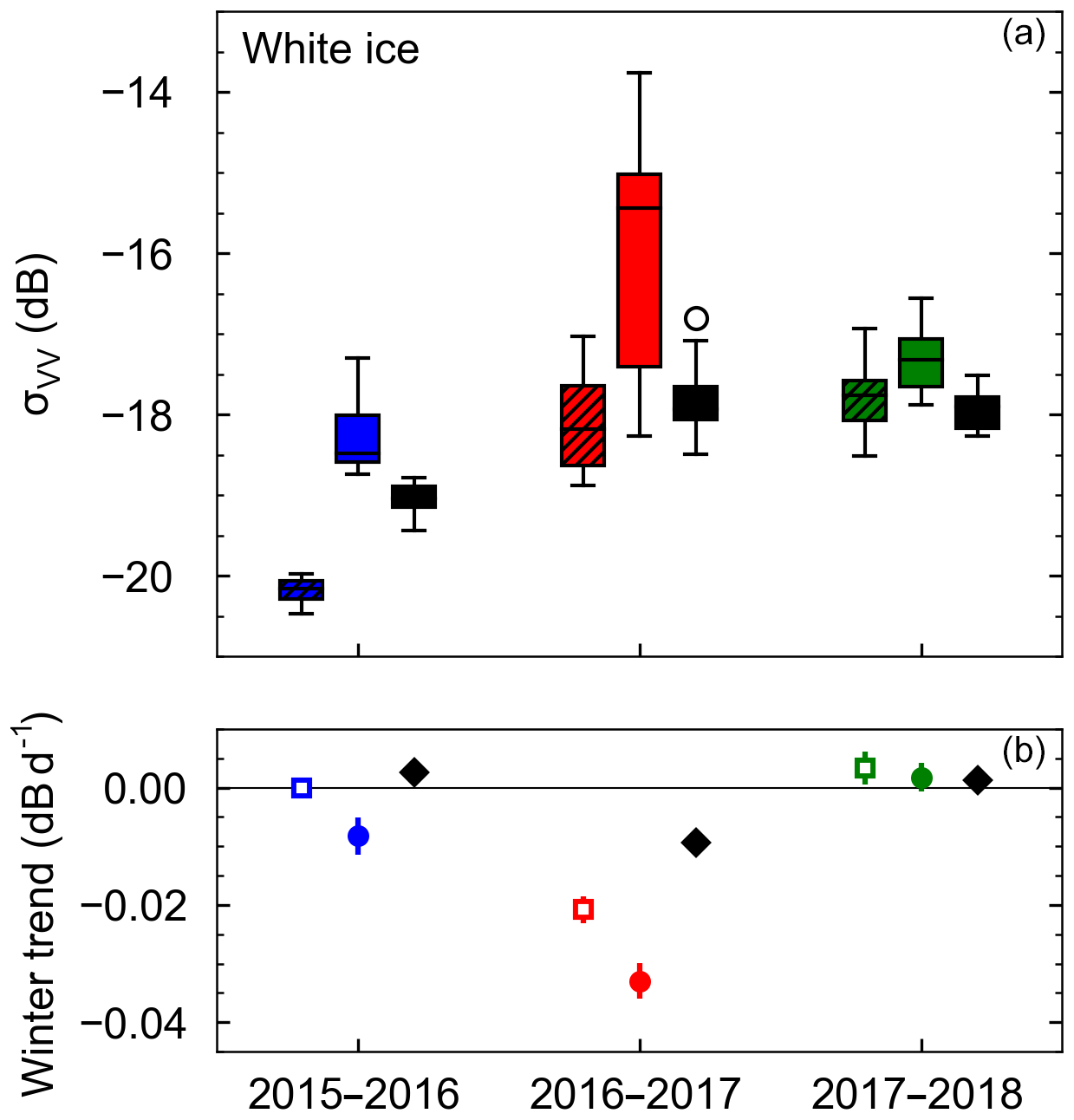
Figure 10Characterization of TerraSAR-X VV winter backscattering. (a) Winter median by year (color coded) for orbits 13 (dashed, ascending, 17:32, 38∘), 21 (solid, descending, 06:25, 40∘), and 89 (black, ascending, 17:40, 46∘). The seasonal median is computed from image medians, which were computed from AOI medians. Empty circle markers represent outliers. (b) Winter trend by year (color coded), for orbits 13 (empty square), 21 (circle), and 89 (black diamond). A horizontal black line indicates the point of zero trend. The trend is defined as the slope of the linear fit to the winter image medians (see Fig. S6). Error bars are the standard error associated with the fit.
5.3 Spring
In the following description of each year's breakup, we refer to zones represented in Fig. 11. The breakup date is the first day when the study area is ice-free.
Figure 11Zones relevant for describing the spatial aspects of breakup in Deception Bay and ship routes for the MV Arctic and MV Nunavik (dashed line). Camera location is indicated with a star.
In 2016, patches of bare ice could be observed throughout the winter, particularly along the southwest shore (zone D). This bare ice started to appear rougher on 20 May. Despite ice-breaking maneuvers performed by the MV Nunavik in zone B upon its arrival in the bay on 16 June, no open water could be seen along its tracks either on the photographs or on the TerraSAR-X image from the same day. Deception River thawed by 16 June. Zone D was seen to be covered in meltwater on 18 June, and open water was first observed on 19 June, in front of the river (zone A). Open water progressed steadily throughout zone B over the course of 5 d, until Moosehead Island (zone C) was also ice-free and breakup was completed on 24 June 2016.
In 2017, snow rapidly melted off following the end of the monotone backscattering period. By 13 May, more than two-thirds of zone B was snow-free, before a snowfall event on 14 May. On 31 May, the ice featured meltwater ponds. Deception River had thawed by 3 June (zone A), and on 4 June some open water could be seen along the ship tracks near zone D. Breakup took 8 d and followed the same spatial pattern as the year before. Breakup was completed with the freeing of zone C on 12 June 2017. In 2018, the snow cover appeared largely melted on the southeastern part of zone B by 28 May, and meltwater was seen on the ice on several occasions in mid-June (zones E). The MV Nunavik and MV Arctic entered the bay on 17 June. Six days later, open water could be seen along most of the ship tracks and the river had thawed. The ships' departure coincided with the first day where meltwater ponds covered the ice. New cracks perpendicular to the shore appeared in the ice that day. These features can be seen on photographs (Fig. 6). Open water was first observed near the southeast shore in zone B on 26 June. The TerraSAR-X image acquired that day (Fig. 6) shows large ice pieces separated along the ship tracks and floating freely in zone B. The breakup was completed on 3 July 2018, 7 d after the first observation of open water.
Figure 12 shows the temporal evolution of the median VV backscattering during the breakup process, as well as indicators derived from time-lapse photography and TerraSAR-X: the end of monotone backscattering (III), the spring peak (IV), and the breakup date. The daily event sequence (Tables S4–S6) – including icebreaker transits, as well as videos assembled from time-lapse photography (Movies S3–S6) and TerraSAR-X (Movies S7–S9) – are all presented in the Supplement and Video supplement. Year 2016 saw both the earliest end of monotone backscattering and the longest period between this and breakup – 59 d compared to 35 in both 2017 and 2018. May 2017 stands out with 57 thawing degree days compared to 4 and 0 in May 2016 and 2018 respectively (see Fig. S10).
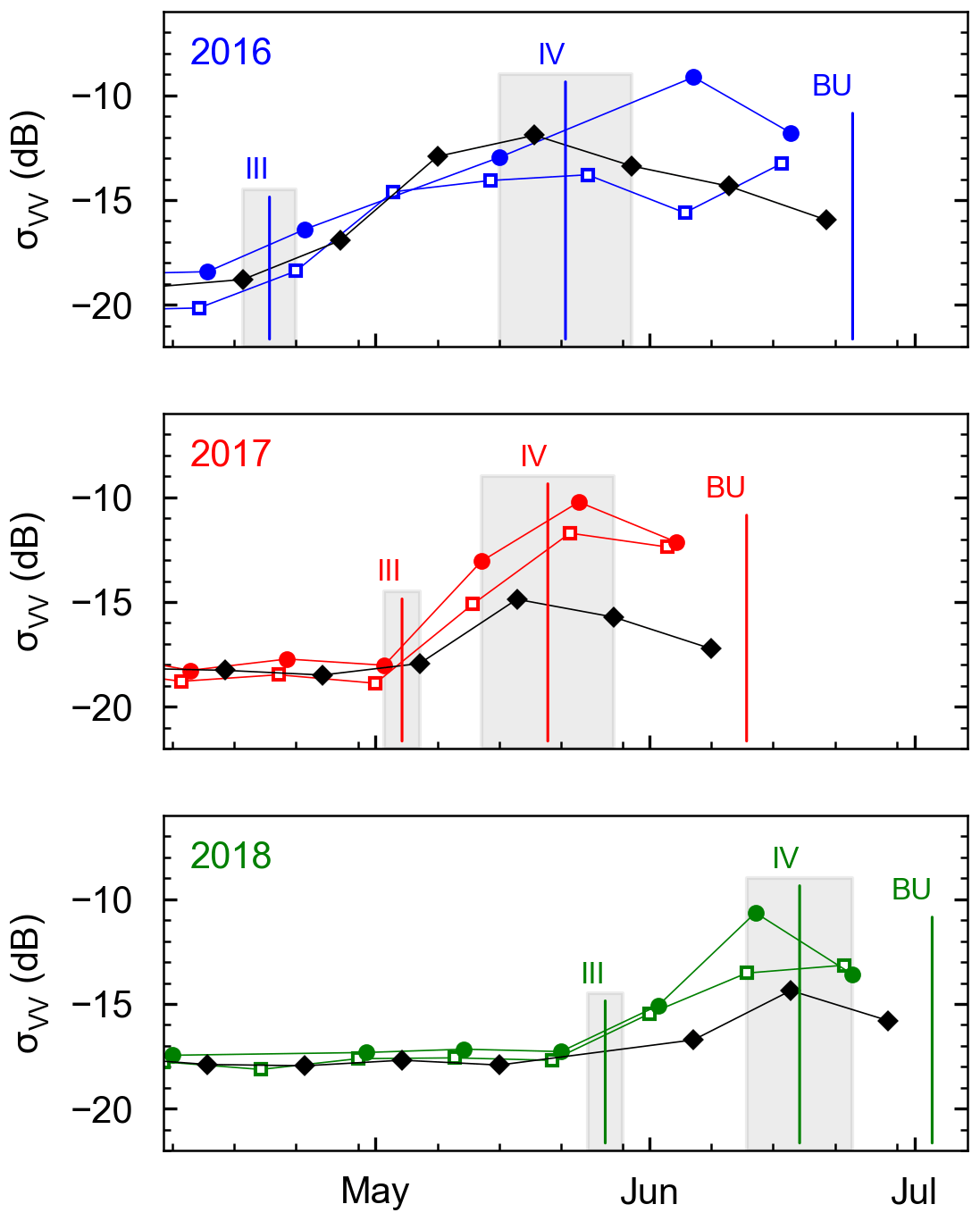
Figure 12TerraSAR-X median VV backscattering is plotted versus time for each year (color coded). Three orbits are shown: orbits 13 (empty square), 21 (circle), and 89 (black diamond). The end of monotone X-band (III, from TerraSAR-X), spring peak (IV, from TerraSAR-X), and the breakup date (BU, from time-lapse photography) are identified with vertical bars. Estimates for each indicator are indicated by shaded gray areas.
The use of TerraSAR-X and time-lapse photography time series for seasonal monitoring of sea ice processes is first discussed for each data source as a stand-alone monitoring tool (Sect. 6.1) and then for their combination (Sect. 6.2). Processes observed in Deception Bay using these tools (freeze-up, wintering, melting and ponding, and breakup) are then discussed in Sect. 6.3.
6.1 Data sources as stand-alone monitoring tools
6.1.1 TerraSAR-X
With a revisit period of 11 d, each TerraSAR-X time series provided access to the seasonal scale of processes. For example, spring features consistently present in all nine datasets for this study (Fig. 12) were associated with springtime melt/thaw processes, as discussed in Sect. 6.3.3. Faster processes could not be resolved, such as freeze-up which unfolded over 1 to 3 d (see Sect. 5.1). Spatially, TerraSAR-X offered the advantage of uniform coverage for the whole study area. This allowed us to document the 2018 breakup spatial pattern (Fig. 6). Success on this front is, however, dependent on lucky timing. Interpretation of the spectral aspect of sea ice processes was hindered by the relative lack of literature specific to X-band backscattering. Indeed, despite their spectral proximity, the C band and X band have been shown to behave differently when it comes to interaction with brine-wetted snow for instance (Nandan et al., 2016, 2017). A study of X-band scattering mechanisms and the associated physiochemical properties of snow and sea ice, although needed, is outside the scope of this paper.
6.1.2 Time-lapse photography
Hourly photographs allowed for the detailed observation of daily or weekly processes, for instance freeze-up. Observations were limited by the absence of photographs during the night and by low visibility periods caused by fog or blowing snow. Spatially, interpretation was limited to the camera's field of view. Details too small (e.g., frost flowers) or too far away (melting of Deception River) could not be resolved. Distances were hard to evaluate on the photographs, which limited the interpretation of feature size or of their extent on the bay (e.g., melt ponds). As for the spectral manifestation of processes, interpretation was straightforward because the photographs were in the visible spectrum. This also allowed for the observation of some meteorological conditions like snowfall (see Tables S1–S6).
6.2 Complementarity of the data sources
The combination of TerraSAR-X and time-lapse photography allowed us to use the strengths of one data source to mitigate weaknesses from another. For example, the TerraSAR-X images acquired during the breakup processes filled in some gaps regarding the state of Deception River (frozen or thawed), which was too far to be resolved on the photographs. Conversely, photography allowed us to compile a daily event sequence of breakup-related events (Tables S3–S6). Overlap of the data sources (e.g., Fig. 6) allowed for cointerpretation, which was used to document the X-band backscattering signature of several newly formed ice types (see Fig. 8), as discussed in Sect. 6.3.1.
6.3 Sea ice processes observed in Deception Bay
6.3.1 Freeze-up
Two different freeze-up processes were documented over the course of the study, as presented in Sect. 5.1. In 2015, calm waters allowed for a quick thermal freeze-up. Below-zero temperatures were earliest in 2015, with the coldest months of October, November, and December of the 3 years (see Fig. S10). In 2016 and 2017, freeze-up rather proceeded iteratively, from patches of nilas and ice rind. We speculate that the first process produced smoother ice than the second process. For a given incidence angle, winter backscattering was systematically lower in 2015–2016 than in the other 2 years (Fig. 10), which we attribute to a smaller surface scattering component that year.
We presented values of dB for grease ice and dB for nilas in VV at 38 to 46∘ (Fig. 8), which is higher than the dB value reported by Nakamura et al. (2005) for new ice (defined as including frazil, grease ice, and nilas), observed in the same polarization and similar incidence angles of 39 to 44∘. Our values are also higher than the −21 dB value reported by Matsuoka et al. (2001) for snow-free thin ice (defined as including nilas and gray ice) observed in HH at lower incidence angles of 22 to 25∘. The backscattering signature of grease ice, which may form waves in the presence of wind, may depend on environmental conditions (Isleifson et al., 2010), which limits comparison. Several factors may be intervening in backscattering from nilas. In cold and dry snow conditions, the X band is not expected to penetrate significantly in the ice cover, with backscattering dominated by the presence of brine at the snow–ice interface (Nandan et al., 2016). Frost flowers are known to increase the backscattering from newly formed sea ice in the C band, an effect which may be more pronounced over thin ice; an increase of 5 dB was reported over ice 2 to 15 cm thick (Nghiem et al., 1997) and of 13 dB over 5 cm thick ice (Isleifson et al., 2014). Snow may also lead to an increase in backscattering through warming of the snow–ice interface and an associated increase in brine scatterer size (Gill et al., 2015). In the case of our nilas observations, snow itself might be enough to explain the 3 dB difference; frost flowers may also have played a role but could not be observed on the photographs.
Despite a difference of almost 20∘ in the incidence angle, our observation of dB over unidentified ice 1 to 9 d after freeze-up (Fig. 8) is close to reports by Johansson et al. (2017) of −11.9 dB over new ice (defined as including nilas, gray ice, and white ice up to 50 cm thick) observed in the X-band VV at 25∘, as well as to reports by Onstott (1992) of −14.4 dB over thin first-year ice (30 to 70 cm thick) in the X-band HH at 23∘. The post-freeze-up peak and monotone backscattering onset are also observed in C-band time series over sea ice (Yackel et al., 2007), but these seasonal features have been less studied than their spring counterparts (end of monotone backscattering and spring peak). Moreover, similar features observed in X- and C-band time series could well be related to different scattering mechanisms, and even to different physical processes. We limit ourselves to speculating, for the X-band data presented in this paper, that the increasing portion of the backscattering peak may be associated with the domination of surface scattering related to a brine-rich ice surface, potentially covered in frost flower, and that the decreasing portion may be associated with a transition to an absorption regime, in which the signal suffers loss in the brine-wetted and increasingly colder snow.
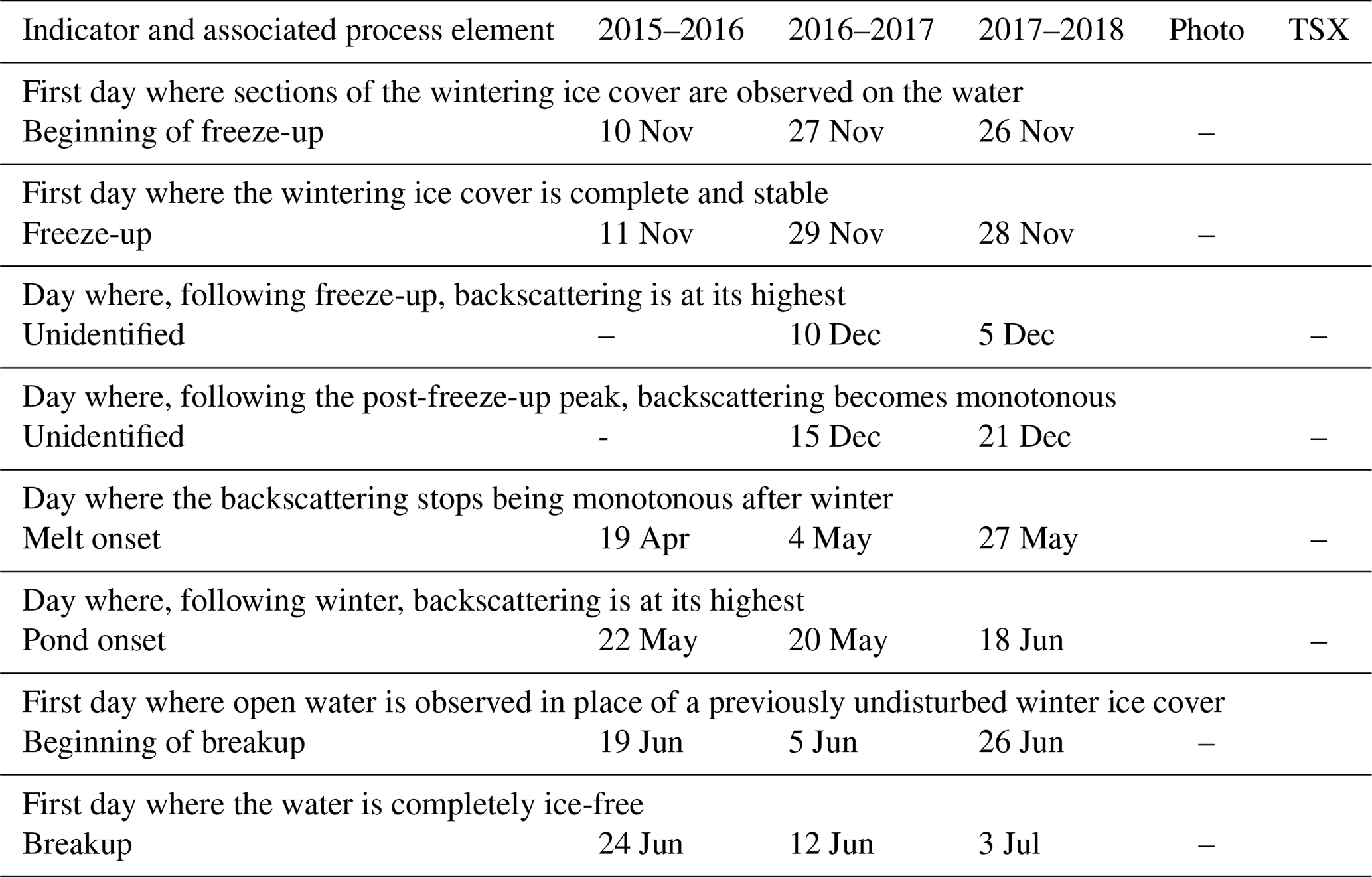
Table 2Seasonal timeline for snow-covered sea ice for 3 years. Process elements derived from time-lapse photography (Photo), and TerraSAR-X (TSX) indicators.
6.3.2 Wintering
Although specific winter sea ice processes exist, for instance sea ice desalination, snow accumulation, and reorganization, time-lapse photography did not allow us to document them. TerraSAR-X time series may however have potential for such monitoring, although another source of data is needed to support interpretation. In general, our backscattering time series fall within the −10 and −20 dB range reported by Onstott (1992) for first-year ice observed with X-band HH or VV at 40∘ between January and June.
Before moving on to the spring processes, we first discuss the influence of an 8∘ difference between ascending orbits 13 and 89. For 2016–2017 and 2017–2018, a small incidence angle effect was seen during the post-freeze-up and spring peaks, where backscattering was 1 to 3 dB smaller at the higher incidence angle (see Figs. 9 and 12), while none was seen during the monotone winter period (see Fig. 10). A backscattering signal which decreases with incidence angle is expected for situations dominated by surface scattering on a relatively rough surface (Ulaby et al., 1986). In the C band, surface scattering at the interfaces between dry snow, brine-wetted snow, and ice is indeed expected to dominate for cold snow-covered sea ice, with a transition to mixed scattering for thicker snow covers (Gill et al., 2015). We speculate that surface scattering explains the small incidence angle effect observed in our X-band data. Mahmud et al. (2018) recently modeled the linear decrease with incidence angle of L- and C-band HH backscattering (in dB) from first-year ice; their results show a dependence of −0.22 dB per degree. This would yield 1.8 dB for an 8∘ difference in the C-band and HH polarization, which is similar to what we observe in the X-band and VV polarization for 2 out of the 3 years. Winter 2015–2016, however, presents a very different case. Backscattering at the higher incidence angle is consistently 2 dB higher than at the lower incidence angle, throughout winter and during the spring peak (see Fig. 12). The freeze-up process was different that year compared to 2016 and 2017, and we have already suggested that the ice cover was much smoother for the 2015–2016 season. We speculate that surface scattering was comparatively low that year and that volume scattering, which Ulaby et al. (1986) have shown can slightly increase with incidence angle, dominated instead.
An acquisition time effect can be seen in the winter data (Fig. 10): the descending/morning winter median was systematically higher than in either ascending/evening orbits. Temperatures in the snow and ice covers are expected to be higher following daytime than in the morning. Dielectric loss in the C band is known to increase with temperature for snow on sea ice (Gill et al., 2015). We speculate that backscattering might be lower in general in the evening than in the morning due to increased dispersion in the warmer medium.
6.3.3 Melting and ponding
Monotone X-band backscattering was observed every winter of the study, for all incidence angles and acquisition times, before a systematic springtime increase in backscattering. In the C band, winter is also characterized by monotone backscattering, ending with melt onset brought on by warmer air temperatures (Yackel et al., 2007). Mechanisms which may increase C-band backscattering from snow-covered sea ice include surface scattering from the brine-wetted layer at the bottom of the snowpack (Nandan et al., 2016), volume scattering on brine inclusions enlarged by an increase in temperature (Barber and Nghiem, 1999), and surface scattering on wet snow (Gill et al., 2015; Yackel et al., 2007) accumulated at the top of the snowpack due to above-zero temperatures and solar radiation (Gogineni et al., 1992; Kim et al., 1984). We speculate that the X band is susceptible to all of these C-band mechanisms, with an emphasis on surface scattering due to its lower penetration depth (Nandan et al., 2016), and attribute the end of X-band monotone backscattering to melt onset.
Springtime backscattering was seen to eventually peak in all TerraSAR-X datasets (Fig. 12), although one series featured more than one maximum (orbit 13, 2015–2016), another none (orbit 13, 2017–2018), and an apparent mismatch between maximum location in the 2015–2016 data. In the C band, springtime peaking of the backscattering is attributed to the transition from the pendular regime (Yackel et al., 2007; Barber et al., 1995), where water is held in the snowpack (Scharien et al., 2012) and backscattering increases as described in the last paragraph, to the funicular regime where meltwater drains downward (Scharien et al., 2012), flushing out brine (Barber et al., 1995) and potentially refreezing (Gogineni et al., 1992). The decrease in C-band backscattering, which forces its peaking, is attributed to a decrease in the dielectric constant of the snowpack following the transition to the funicular regime (Yackel et al., 2007). We speculate that the decrease in the X-band springtime backscattering is also caused by pond onset and associated with increased penetration in the drained snowpack.
Neither melt nor pond onset could be resolved using time-lapse photography, although signs of ice cover degradation were eventually observed and used to document breakup (see example in Fig. 5). Table 2 shows melt and pond onset timing estimated by combining the three TerraSAR-X time series. Year 2016 showed the earliest melt onset and the longest period separating it from pond onset (33 d). Year 2017 showed the shortest time separating melt onset from pond onset (16 d) and the earliest pond onset of the 3 years. Year 2018 showed the latest melt and pond onsets, separated by 22 d. This is consistent with air temperature data from Salluit Airport; 2018 had the coldest months of May and June (see Fig. S3–3). Meltwater was observed on the ice surface 27 and 11 d after pond onset in 2016 and 2017, respectively, and the day before in 2018, as shown in Tables S4–S6.
6.3.4 Breakup
Two different breakup processes were observed over the course of the study, as presented in Sect. 5.3. In 2016 and 2017, open water was first observed near Deception River, and its extent progressed towards the rest of the bay until the whole study area was ice-free. This contrasts with 2018 where, although open water was also first observed near Deception River, breakup was rather characterized by the presence of large ice floes which floated in the bay for a week before disappearing overnight, signalling breakup completion. In 2016, breakup began 3 d after the MV Nunavik first entered the bay in the spring. The first ice-breaking transit of the season occurred respectively 3 d before and 1 d after the beginning of breakup 2016 and 2017. The 2016 breakup started 28 d after pond onset, compared to the 16 d period observed in 2017. We speculate that the ice cover was in a more advanced state of degradation when breakup started in 2016 than in 2017. This is supported by time-lapse photography which shows that the ice cover was partly mobile (under the effect of wind or current) during breakup in 2016 but mostly landfast during breakup in 2017 (Movies S4–S5). In 2018's comparatively late spring, both the MV Nunavik and MV Arctic entered the bay during pond onset (on 17 June). Open water was observed along their tracks in the following days, and new cracks perpendicular to the shore appeared when the ships left the bay 8 d later. In 2016 and 2017, the last area to be cleared of ice was Moosehead Island and its shallows.
With the data available, it is hard to evaluate the impact of shipping on the breakup process in Deception Bay, be it on its pattern, timing, or length. What we can say is that (1) the breakup spatial pattern followed shipping tracks in 2018 but did not in 2016 and 2017; (2) breakup lasted 5, 7, and 7 d in 2016, 2017, and 2018, respectively; and (3) it was completed respectively 33, 23, and 15 d after pond onset. Future work on this front would do well to consider the melting of the ice from underneath due to currents, an important aspect of breakup (Laidler and Ikummaq, 2008) which is hard to access using TerraSAR-X and time-lapse photography.
6.3.5 Seasonal timeline and caveats
Table 2 presents a timeline for the elements relating to sea ice processes which were studied using TerraSAR-X and time-lapse photography indicators. Two indicators derived from backscattering time series could not be associated with specific elements of sea ice processes: these are the post-freeze-up peak and the beginning of the monotone X band.
This seasonal timeline relies on the assumptions that (1) freeze-up, wintering, and breakup processes occur each year; that (2) despite interannual differences in timing and spatial extent, the process elements listed in Table 2 always occur; and that (3) the TerraSAR-X and time-lapse photography time series indicators are always a manifestation of these process elements. This may not always be the case; for instance, melting and ponding is known to be hard to resolve in the C band for thin ice covers (Yackel et al., 2007), and two of the X-band-derived indicators could not be reliably associated with process elements.
This article presented a case study for the seasonal monitoring of sea ice processes using a combination of TerraSAR-X and time-lapse photography time series. The two data sources proved complementary, with their combination enabling spatiotemporal coverage of the processes. It also led to the reporting of new X-band backscattering values over newly formed sea ice types. TerraSAR-X time series showed potential for tracking melt and pond onset. Finally, we documented two types of freeze-up and breakup processes for Nunavik's Deception Bay, an area at the confluence of climate change, land use by local Inuit, and ice-breaking transport by the mining industry. These processes were seen to depend on geomorphological features such as Moosehead Island and Deception River. Future work in the Ice Monitoring project will build on this characterization of seasonal processes and focus on spatial variations within the bay and comparison with similar fjords, namely Salluit and Kangiqsujuaq. It will also involve comparison of the TerraSAR-X time series data with RADARSAT-2 time series acquired over the same period and area.
Code and data availability. The complete time-lapse photography database can be accessed at http://caiman.ete.inrs.ca (Bernier et al., 2017). Quicklooks for the TerraSAR-X images as well as freeze-up and breakup event sequences are available on https://doi.org/10.1594/PANGAEA.904960 (Dufour-Beauséjour et al., 2019). The code used to compute pixel statistics from the TerraSAR-X images on areas of interest is available at https://github.com/sdufourbeausejour/tiffstats (last access: 20 May 2020; sdufourbeausejour, 2020).
The supplement related to this article is available online at: https://doi.org/10.5194/tc-14-1595-2020-supplement.
Movies S1, S2, and S3 respectively show the freeze-up sequence for 2015, 2016, and 2017. Movies S4, S5, and S6 respectively show the breakup sequence for 2016, 2017, and 2018. Movies S7, S8, and S9 respectively show the TerraSAR-X image time series (all orbits combined) for the 2015–2016, 2016–2017, and 2017–2018 ice seasons. They are available online at https://doi.org/10.1594/PANGAEA.904960 (Dufour-Beauséjour et al., 2019).
SD-B participated in study design, data acquisition, analysis, and interpretation and wrote the article. AW participated in study design, data analysis, and interpretation and wrote the article. YG participated in study design and data interpretation and revised the article. MB participated in study design and revised the article. JP and VG participated in study design and data acquisition. JT and AcR participated in data acquisition. AmR participated in study design.
The authors declare that they have no conflict of interest.
The authors would like to thank the Inuit guides from Salluit who participated in data acquisition in Deception Bay (in alphabetical order): Chris Alaku, Johnny Ashevak, Michael Camera, Putulik Cameron, Charlie Ikey, Luuku Isaac, Markusi Jaaka, Adamie Raly Kadjulik, Joannasie Kakayuk, Jani Kenuajuak, Pierre Lebreux, Casey Mark, Denis Napartuk, Eyetsiaq Papigatuk, and Kululak Tayara. Thanks also to INRS students who also participated in data acquisition: Pierre-Olivier Carreau, and Étienne Lauzier-Hudon. Thanks to Jasmin Gill-Fortin (INRS) for his help with the time-lapse photography data. We further thank Valérie Plante Lévesque (INRS), Charles Gignac (INRS), Randy Scharien (University of Victoria), Torsten Geldsetzer (Natural Resources Canada), and Derek Mueller (Carleton University) for their advice and suggestions on this paper, as well as Guillaume Légaré (INRS) for his advice on time series analysis. Thanks also to the anonymous reviewers, whose comments greatly improved this article, and to the editorial team. Thanks to the German Space Agency (DLR) for providing the TerraSAR-X images and for data processing with the Multi-SAR-System. The authors acknowledge the use of TerraSAR-X (© DLR 2017-18). This study was done within the Ice Monitoring project, a research collaboration between the Kativik Regional Government (KRG); Raglan Mine, a Glencore company; Institut national de la recherche scientifique (INRS); and the Northern Villages of Salluit and Kangiqsujuaq.
This research has been supported by Polar Knowledge Canada (grant no. PKCNST-1617-0003); Raglan Mine, a Glencore company (Raglan Mine–KRG contract no. 1459 and Raglan Mine–KRG contract no. 2330); the Kativik Regional Government (Raglan Mine–KRG contract no. 1459); NSERC (Discovery Grant and Northern Research Supplements Program grant); and the Ministère des Transports du Québec (grant no. Fonds vert – CC09.1, 2015). Scholarships were attributed to Sophie Dufour-Beauséjour by NSERC (Alexander Graham Bell Canada Graduate Scholarship – Doctoral), the W. Garfield Weston Foundation (the W. Garfield Weston Awards in Northern Research), and the Northern Scientific Training Program.
This paper was edited by Dirk Notz and reviewed by three anonymous referees.
Arslan, A. N., Tanis, C. M., Metsämäki, S., Aurela, M., Böttcher, K., Linkosalmi, M., and Peltoniemi, M.: Automated Webcam Monitoring of Fractional Snow Cover in Northern Boreal Conditions, Geosciences, 7, 55, https://doi.org/10.3390/geosciences7030055, 2017.
Barber, D. G. and Nghiem, S. V.: The role of snow on the thermal dependence of microwave backscatter over sea ice, J. Geophys. Res.-Oceans, 104, 25789–25803, https://doi.org/10.1029/1999JC900181, 1999.
Barber, D. G., Papakyriakou, T. N., Ledrew, E. F., and Shokr, M. E.: An examination of the relation between the spring period evolution of the scattering coefficient (σ) and radiative fluxes over Jandfast sea-ice, Int. J. Remote Sens., 16, 3343–3363, https://doi.org/10.1080/01431169508954634, 1995.
Bernier, M., Poulin, J., Gilbert, V., and Rouleau, A.: Ice Monitoring: Hourly pictures of landfast sea ice from Deception Bay (Nunavik, Canada), Canadian Cryospheric Information Network (CCIN), 2017.
Bertram, A., Wendleder, A., Schmitt, A., and Huber, M.: Long-Term Monitoring of Water Dynamics in the Sahel Region using the Multi-SAR-System, in: The International Archives of the Photogrammetry, Remote Sensing and Spatial Information Sciences, XXIII ISPRS Congress, Commission VIII, Prague, Czech Republic, 12–19 July 2016, 8 pp., 2016.
Bongio, M., Arslan, A. N., Tanis, C. M., and De Michele, C.: Snow depth estimation by time-lapse photography: Finnish and Italian case studies, The Cryosphere Discuss., https://doi.org/10.5194/tc-2019-193, in review, 2019.
Cassotto, R., Fahnestock, M., Amundson, J. M., Truffer, M., and Joughin, I.: Seasonal and interannual variations in ice melange and its impact on terminus stability, Jakobshavn Isbræ, Greenland, J. Glaciol., 61, 76–88, https://doi.org/10.3189/2015JoG13J235, 2015.
Chauché, N., Hubbard, A., Gascard, J.-C., Box, J. E., Bates, R., Koppes, M., Sole, A., Christoffersen, P., and Patton, H.: Ice–ocean interaction and calving front morphology at two west Greenland tidewater outlet glaciers, The Cryosphere, 8, 1457–1468, https://doi.org/10.5194/tc-8-1457-2014, 2014.
Christiansen, H. H.: Snow-cover depth, distribution and duration data from northeast Greenland obtained by continuous automatic digital photography, Ann. Glaciol., 32, 102–108, https://doi.org/10.3189/172756401781819355, 2001.
Cuerrier, A., Brunet, N. D., Gérin-Lajoie, J., Downing, A., and Lévesque, E.: The Study of Inuit Knowledge of Climate Change in Nunavik, Quebec: A Mixed Methods Approach, Hum. Ecol., 43, 379–394, https://doi.org/10.1007/s10745-015-9750-4, 2015.
Dufour-Beauséjour, S., Wendleder, A., Gauthier, Y., Bernier, M., Poulin, J., Gilbert, V., Tuniq, J., and Rouleau, A.: (Movie S1–S6) Freeze-up and break-up observations in Nunavik's Deception Bay from TerraSAR-X and time-lapse photography, PANGAEA, https://doi.org/10.1594/PANGAEA.904960, 2019.
Dumont, M., Sirguey, P., Arnaud, Y., and Six, D.: Monitoring spatial and temporal variations of surface albedo on Saint Sorlin Glacier (French Alps) using terrestrial photography, The Cryosphere, 5, 759–771, https://doi.org/10.5194/tc-5-759-2011, 2011.
Eineder, M., Fritz, T., Mittermayer, J., Roth, A., Boerner, E., and Breit, H.: TerraSAR-X Ground Segment, Basic Product Specification Document, CAF – Cluster Applied Remote Sensing, Germany, 2008.
Eriksson, L. E. B., Pemberton, P., Lindh, H., and Karlson, B.: Evaluation of new spaceborne SAR sensors for sea-ice monitoring in the Baltic Sea, Can. J. Remote Sens., 36, S56–S73, https://doi.org/10.5589/m10-020, 2010.
Farinotti, D., Magnusson, J., Huss, M., and Bauder, A.: Snow accumulation distribution inferred from time-lapse photography and simple modelling, Hydrol. Process., 24, 2087–2097, https://doi.org/10.1002/hyp.7629, 2010.
Fequet, D., Hache, L., McCourt, S., Langlois, D., Dicaire, C., Premont, B., Jolicoeur, A., and Minano, A.: Sea Ice Climatic Atlas: Northern Canadian Waters 1981–2010, En56-173-2010–1, Canadian Ice Service, Environnement Canada, Ottawa, Ont., 2011.
Fors, A. S., Brekke, C., Doulgeris, A. P., Eltoft, T., Renner, A. H. H., and Gerland, S.: Late-summer sea ice segmentation with multi-polarisation SAR features in C and X band, The Cryosphere, 10, 401–415, https://doi.org/10.5194/tc-10-401-2016, 2016.
Gauthier, Y., Dufour-Beauséjour, S., Poulin, J., and Bernier, M.: Ice Monitoring in Deception Bay?: Progress report 2016-2018, Québec: INRS, Centre Eau Terre Environnement, available at: http://espace.inrs.ca/7538/ (last access: 15 May 2020), 2018.
GENIVAR: Environmental and Social Impact Assessment of the Deception Bay Wharf and Sediment Management, Report from GENIVAR for Canadian Royalties Inc., Montreal, Que., 2012.
Gill, J. P. S., Yackel, J. J., Geldsetzer, T., and Fuller, M. C.: Sensitivity of C-band synthetic aperture radar polarimetric parameters to snow thickness over landfast smooth first-year sea ice, Remote Sens. Environ., 166, 34–49, https://doi.org/10.1016/j.rse.2015.06.005, 2015.
Gogineni, S. P., Moore, R. K., Grenfell, T. C., Barber, D., Digby, S., and Drinkwater, M.: The effects of freeze-up and melt processes on microwave signatures, in Microwave remote sensing of sea ice, Geophys. Monogr., Vol. 68, edited by: Carsey, F. D., 329–334, Washington, DC, 1992.
Herdes, E., Copland, L., Danielson, B., and Sharp, M.: Relationships between iceberg plumes and sea-ice conditions on northeast Devon Ice Cap, Nunavut, Canada, Ann. Glaciol., 53, 1–9, https://doi.org/10.3189/2012AoG60A163, 2012.
Ide, R. and Oguma, H.: A cost-effective monitoring method using digital time-lapse cameras for detecting temporal and spatial variations of snowmelt and vegetation phenology in alpine ecosystems, Ecol. Inform., 16, 25–34, https://doi.org/10.1016/j.ecoinf.2013.04.003, 2013.
Isleifson, D., Hwang, B., Barber, D. G., Scharien, R. K., and Shafai, L.: C-Band Polarimetric Backscattering Signatures of Newly Formed Sea Ice During Fall Freeze-Up, IEEE T. Geosci. Remote, 48, 3256–3267, https://doi.org/10.1109/TGRS.2010.2043954, 2010.
Isleifson, D., Galley, R. J., Barber, D. G., Landy, J. C., Komarov, A. S., and Shafai, L.: A Study on the C-Band Polarimetric Scattering and Physical Characteristics of Frost Flowers on Experimental Sea Ice, IEEE Trans. Geosci. Remote Sens., 52, 1787–1798, https://doi.org/10.1109/TGRS.2013.2255060, 2014.
Johansson, A. M., King, J. A., Doulgeris, A. P., Gerland, S., Singha, S., Spreen, G., and Busche, T.: Combined observations of Arctic sea ice with near-coincident colocated X-band, C-band, and L-band SAR satellite remote sensing and helicopter-borne measurements, J. Geophys. Res.-Oceans, 122, 669–691, https://doi.org/10.1002/2016JC012273, 2017.
Johansson, A. M., Brekke, C., Spreen, G., and King, J. A.: X-, C-, and L-band SAR signatures of newly formed sea ice in Arctic leads during winter and spring, Remote Sens. Environ., 204, 162–180, https://doi.org/10.1016/j.rse.2017.10.032, 2018.
Kępski, D., Luks, B., Migała, K., Wawrzyniak, T., Westermann, S., and Wojtuń, B.: Terrestrial remote sensing of snowmelt in a diverse High-Arctic tundra environment using time-lapse imagery, Remote Sens., 9, 733, https://doi.org/10.3390/rs9070733, 2017.
Kim, Y.-S., Onstott, R., and Moore, R.: Effect of a snow cover on microwave backscatter from sea ice, IEEE J. Oceanic Eng., 9, 383–388, https://doi.org/10.1109/JOE.1984.1145649, 1984.
Laidler, G. J. and Ikummaq, T.: Human Geographies of Sea Ice: Freeze/Thaw Processes around Igloolik, Nunavut, Canada, Polar Rec., 44, 127–153, https://doi.org/10.1017/S0032247407007152, 2008.
Liu, J., Chen, R., Song, Y., Yang, Y., Qing, W., Han, C., and Liu, Z.: Observations of precipitation type using a time-lapse camera in a mountainous region and calculation of the rain/snow proportion based on the critical air temperature, Environ. Earth Sci., 73, 1545–1554, https://doi.org/10.1007/s12665-014-3506-0, 2015.
Mahmud, M. S., Geldsetzer, T., Howell, S. E. L., Yackel, J., Nandan, V., and Scharien, R. K.: Incidence Angle Dependence of HH-Polarized C- and L-Band Wintertime Backscatter Over Arctic Sea Ice, IEEE Trans. Geosci. Remote Sens., 56, 6686–6698, https://doi.org/10.1109/TGRS.2018.2841343, 2018.
Mailhot, A. and Chaumont, D.: Élaboration du portrait bioclimatique futur du Nunavik – Tome II. Rapport présenté au Ministère de la forêt, de la faune et des parcs, Ouranos, Montreal, Que., 2017.
Matsuoka, T., Uratsuka, S., Satake, M., Kobayashi, T., Nadai, A., Umehara, T., Maeno, H., Wakabayashi, H., Nakamura, K., and Nishio, F.: CRL/NASDA airborne SAR (Pi-SAR) observations of sea ice in the Sea of Okhotsk, Ann. Glaciol., 33, 115–119, https://doi.org/10.3189/172756401781818734, 2001.
Mussells, O., Dawson, J., and Howell, S.: Navigating Pressured Ice: Risks and Hazards for Winter Resource-Based Shipping in the Canadian Arctic, Ocean Coast. Manage., 137, 57–67, https://doi.org/10.1016/j.ocecoaman.2016.12.010, 2017.
Nakamura, K., Wakabayashi, H., Naoki, K., Nishio, F., Moriyama, T., and Uratsuka, S.: Observation of sea-ice thickness in the sea of Okhotsk by using dual-frequency and fully polarimetric airborne SAR (pi-SAR) data, IEEE T. Geosci. Remote, 43, 2460–2469, https://doi.org/10.1109/TGRS.2005.853928, 2005.
Nandan, V., Geldsetzer, T., Islam, T., Yackel, John. J., Gill, J. P. S., Fuller, Mark. C., Gunn, G., and Duguay, C.: Ku-, X- and C-band measured and modeled microwave backscatter from a highly saline snow cover on first-year sea ice, Remote Sens. Environ., 187, 62–75, https://doi.org/10.1016/j.rse.2016.10.004, 2016.
Nandan, V., Geldsetzer, T., Mahmud, M., Yackel, J., and Ramjan, S.: Ku-, X-and C-Band Microwave Backscatter Indices from Saline Snow Covers on Arctic First-Year Sea Ice, Remote Sens., 9, 757, https://doi.org/10.3390/rs9070757, 2017.
Nghiem, S. V., Martin, S., Perovich, D. K., Kwok, R., Drucker, R., and Gow, A. J.: “A Laboratory Study of the Effect of Frost Flowers on C Band Radar Backscatter from Sea Ice.”, J. Geophys. Res.-Oceans, 102, 3357–3370, https://doi.org/10.1029/96JC03208, 1997.
Nickels, S., Furgal, C., Buell, M., and Moquin, H.: Unikkaaqatigiit – Putting the Human Face on Climate Change: Perspectives from Inuit in Canada, Pre-release English only version, Inuit Tapiriit Kanatami, Nasivvik Centre for Inuit Health and Changing Environments at Université Laval and the Ajunnginiq Centre at the National Aboriginal Health Organization, Ottawa, Ont., 2005.
Onstott, R. G.: SAR and Scatterometer Signatures of Sea Ice, in: Microwave Remote Sensing of Sea Ice, American Geophysical Union, Washington, D.C., United States, 73–104, 1992.
Paul, S., Willmes, S., Hoppmann, M., Hunkeler, P. A., Wesche, C., Nicolaus, M., Heinemann, G., and Timmermann, R.: The impact of early-summer snow properties on Antarctic landfast sea-ice X-band backscatter, Ann. Glaciol., 56, 263–273, https://doi.org/10.3189/2015AoG69A715, 2015.
Peltoniemi, M., Aurela, M., Böttcher, K., Kolari, P., Loehr, J., Karhu, J., Linkosalmi, M., Tanis, C. M., Tuovinen, J.-P., and Arslan, A. N.: Webcam network and image database for studies of phenological changes of vegetation and snow cover in Finland, image time series from 2014 to 2016, Earth Syst. Sci. Data, 10, 173–184, https://doi.org/10.5194/essd-10-173-2018, 2018.
Petit, J.-G., Viger, Y. B., Aatami, P., and Iserhoff, A.: Les Inuit et les Cris du Nord du Québec: Territoire, gouvernance, société et culture, PUQ, Quebec, Que., 2011.
Revuelto, J., Jonas, T., and López-Moreno, J.-I.: Backward snow depth reconstruction at high spatial resolution based on time-lapse photography, Hydrol. Process., 30, 2976–2990, https://doi.org/10.1002/hyp.10823, 2016.
Scharien, R. K., Yackel, J. J., Barber, D. G., Asplin, M., Gupta, M., and Isleifson, D.: Geophysical controls on C band polarimetric backscatter from melt pond covered Arctic first-year sea ice: Assessment using high-resolution scatterometry, J. Geophys. Res.-Oceans, 117, C00G18, https://doi.org/10.1029/2011JC007353, 2012.
Schmitt, A., Wendleder, A., and Hinz, S.: The Kennaugh element framework for multi-scale, multi-polarized, multi-temporal and multi-frequency SAR image preparation, ISPRS J. Photogramm., 102, 122–139, https://doi.org/10.1016/j.isprsjprs.2015.01.007, 2015.
sdufourbeausejour: tiffstats, available at: https://github.com/sdufourbeausejour/tiffstats, last access: 20 May 2020.
Smith Jr., K. L., Baldwin, R. J., Glatts, R. C., Chereskin, T. K., Ruhl, H., and Lagun, V.: Weather, ice, and snow conditions at Deception Island, Antarctica: long time-series photographic monitoring, Deep-Sea Res. Pt. II, 50, 1649–1664, https://doi.org/10.1016/S0967-0645(03)00084-5, 2003.
Sobiech, J., Boike, J., and Dierking, W.: Observation of melt onset in an arctic tundra landscape using high resolution TerraSAR-X and RADARSAT-2 data, in 2012 IEEE International Geoscience and Remote Sensing Symposium, 3552–3555, 2012.
Stettner, S., Lantuit, H., Heim, B., Eppler, J., Roth, A., Bartsch, A., and Rabus, B.: TerraSAR-X Time Series Fill a Gap in Spaceborne Snowmelt Monitoring of Small Arctic Catchments – A Case Study on Qikiqtaruk (Herschel Island), Canada, Remote Sens., 10, 1155, https://doi.org/10.3390/rs10071155, 2018.
Tuniq, J., Usuituayuk, T., Saviadjuk, P., Papigatuk Lebreux, I., Delisle Alaku, A., and Cameron, M.: Observations of Arctic Change from Salluit, Nunavik, Presented at Arctic Change 2017, Quebec, Canada, 2017.
Ulaby, F. T., Moore, R. K., and Fung, A. K.: Microwave Remote Sensing: Active and Passive. Vol. 3, From theory to applications, Addison-Wesley Publishing Company, Boston, United States, 1986.
Vogel, S., Eckerstorfer, M., and Christiansen, H. H.: Cornice dynamics and meteorological control at Gruvefjellet, Central Svalbard, The Cryosphere, 6, 157–171, https://doi.org/10.5194/tc-6-157-2012, 2012.
WMO: Sea-Ice Nomenclature, No. 259, World Meteorological Organization, Switzerland, 2014.
Wobus, C., Anderson, R., Overeem, I., Matell, N., Clow, G., and Urban, F.: Thermal Erosion of a Permafrost Coastline: Improving Process-Based Models Using Time-Lapse Photography, Arct. Antarct. Alp. Res., 43, 474–484, https://doi.org/10.1657/1938-4246-43.3.474, 2011.
Yackel, J. J., Barber, D. G., Papakyriakou, T. N., and Breneman, C.: First-year sea ice spring melt transitions in the Canadian Arctic Archipelago from time-series synthetic aperture radar data, 1992–2002, Hydrol. Process., 21, 253–265, https://doi.org/10.1002/hyp.6240, 2007.
Zhang, E., Liu, L., and Huang, L.: Automatically delineating the calving front of Jakobshavn Isbræ from multitemporal TerraSAR-X images: a deep learning approach, The Cryosphere, 13, 1729–1741, https://doi.org/10.5194/tc-13-1729-2019, 2019.