the Creative Commons Attribution 4.0 License.
the Creative Commons Attribution 4.0 License.
 | 17 Apr 2020
The influence of water percolation through crevasses on the thermal regime of a Himalayan mountain glacier
Tika R. Gurung
Koji Fujita
Sudan B. Maharjan
Tenzing C. Sherpa
Takehiro Fukuda
In cold and arid climates, small glaciers with cold accumulation zones are often thought to be entirely cold based. However, scattering in ground-penetrating radar (GPR) measurements on the Rikha Samba Glacier in the Nepal Himalayas suggests a large amount of temperate ice that seems to be influenced by the presence of crevassed areas. We used a coupled thermo-mechanical model forced by a firn model accounting for firn heating to interpret the observed thermal regime. Using a simple energy conservation approach, we show that the addition of water percolation and refreezing in crevassed areas explains these observations. Model experiments show that both steady and transient thermal regimes are significantly affected by latent heat release in crevassed areas. This makes half of the glacier base temperate, resulting in an ice dynamic mainly controlled by basal friction instead of ice deformation. The timescale of thermal regime change, in response to atmospheric warming, is also greatly diminished, with a potential switch from cold to temperate basal ice in 50–60 years in the upper part of the glacier instead of the 100–150 years that it would take without the effect of the crevasses. This study highlights the crucial role of water percolation through the crevasses on the thermal regime of glaciers and validates a simple method to account for it in glacier thermo-mechanical models.
- Article
(21767 KB) - Full-text XML
- BibTeX
- EndNote


The thermal regime of a mountain glacier controls its hydrology, flow rheology and basal conditions affecting glacier dynamics, which in turn affect its behaviour in response to climate change. It influences erosion rates (Bennett and Glasser, 2011), potential glacier hazards (Faillettaz et al., 2011; Gilbert et al., 2015) and water resources in the glaciated catchments (Miller et al., 2012). It is thus essential to understand the processes causing and maintaining temperate basal conditions as well as the mechanisms leading to changes in the thermal regime of glaciers.
Very little is known about the thermal regime of the Himalayan glaciers due to the harsh conditions and logistical difficulties which make direct observations challenging in remote, high-altitude areas. Borehole temperature measurements, such as carried out on Khumbu, Yala and Gyabrag glaciers in the Himalayas (Miles et al., 2018; Mae, 1976; Watanabe et al., 1984; Liu et al., 2009), provide direct observations of the glaciers' thermal condition. However, the small number of boreholes gives only very limited information about the spatial distribution of the ice temperatures within the glacier. An estimation of the thermal structure of the glacier in such a case requires the use of numerical modelling in order to extrapolate the borehole measurements (Wang et al., 2018; Zhang et al., 2013).
Scattering of electromagnetic wave signals in glacier ice is commonly regarded as diagnosing temperate ice in ground-penetrating radar (GPR) data. Continuous GPR profiles can thus provide information about the spatial distribution of thermal ice zones within a glacier (e.g. Ryser et al., 2013; Wilson et al., 2013; Gusmeroli et al., 2012; Irvine-Fynn et al., 2006; Pettersson et al., 2007). Wilson et al. (2013) showed that the interface between cold and temperate ice matching with the location of temperatures reaching the pressure melt point in the boreholes could be identified with a 10 MHz GPR on two sub-Arctic polythermal glaciers. In the Himalayas, such GPR data are rare, although Sugiyama et al. (2013) showed with GPR data that the Yala Glacier in Nepal is polythermal, which was in agreement with two previous borehole measurements in the ablation and accumulation areas of the glacier (Watanabe et al., 1984).
In this study, we determine the polythermal structure and ice thickness of a high-altitude glacier in the Nepal Himalayas using GPR. We combine GPR data from 2010 and 2015 with other field data to determine ice thickness and to estimate the amount of temperate versus cold ice in the glacier. Measurements are interpreted using a 3D thermo-mechanical model for which we have developed new methods in order to (i) determine the thermal surface boundary condition and (ii) take into account water percolation and refreezing in the crevassed areas. The model is forced by a surface mass balance model calibrated with field measurements, which is then run to determine the steady-state and transient thermal regimes of the glacier. We compare our modelling results with the GPR data to draw conclusions about the processes defining the thermal regime of the glacier and to provide recommendations on how to take them into account in further modelling studies.
2.1 Study area
The Rikha Samba Glacier is a south-east-orientated, medium-sized glacier (5.5 km2) located in the Hidden Valley in western Nepal (Fig. 1a). The glacier was about 5.5 km long with an elevation ranging from 5420 to 6440 m a.s.l. in 2014. The glacier meltwater contributes to the Kali Gandaki Basin of the Ganges River. The Hidden Valley falls under a rain shadow climate, receiving the least precipitation in Nepal with an annual precipitation of 370 mm (Fujita and Nuimura, 2011). The annual mean temperature measured with an automatic weather station (AWS) in the vicinity of the glacier (Fig. 1a) was −5 ∘C in 2014. The glacier was first visited in 1974 and it had been losing mass at a mean rate of −0.5 m w.e. yr−1 between 1974 and 2010 (Fujita et al., 1997; Fujita and Nuimura, 2011).

Figure 1(a) Location and (b) map of Rikha Samba Glacier in the Hidden Valley catchment in Nepal. Radar tracks in 2015 (red dots), radar point measurements in 2010 (blue circles) and location of the thermistor chain (red diamond) are shown in (b). Background image of (a) is from Landsat 5 on 25 May 2010. Background image of (b) is from Google Earth (image © 2020 Maxar Technologies).
2.2 Ground-penetrating radar (GPR)
We used a Malå GeoScience ProEx impulse-type ground-penetrating radar (GPR) with a 30 MHz rough terrain antenna (RTA) with a frequency band from 15 to 45 MHz to measure the ice thickness and thermal regime of the Rikha Samba Glacier in 2015 (Fig. 1b). The RTA is an unshielded radar antenna in which the transmitter and receiver elements are mounted in a row in a flexible tube, making it suitable for rough terrain such as glacier surfaces.
DC offset was subtracted from the data, and a gain function as well as a bandpass Butterworth filter removing frequencies below 15 MHz and above 45 MHz were applied to the continuous radar profiles. The GPR reflectors from the assumed bedrock surface were manually picked from the data. Picked two-way travel times of the radar signal were converted to ice thickness using a wave velocity of 168 m µs−1 (Robin, 1975). Strong scattering of the radar signal within the ice was interpreted as temperate, ice whereas ice without internal reflectors was classified as cold ice, and the interface between these zones was also manually picked in the data. In addition, we have used point data collected in 2010 with an impulse GPR transmitter (Ohio State University) with a set of half-wavelength 5 MHz dipole antennae (Fig. 1b). These data were used only for ice thickness. The time increment of 5 years between the GPR measurements was corrected by projecting the 2010 data to 2015. This was done by assuming that the glacier was thinning at the same rate between 2010 and 2015 as the long-term thinning rate for 100 m elevation bands obtained for a 12-year period between 1998 and 2010 (Fujita and Nuimura, 2011).
2.3 Glacier geometry and crevasse location
A digital elevation model (DEM) of 30 m resolution was generated for the Rikha Samba Glacier from Pleiades tri-stereo satellite imagery (0.5 m resolution) for 7 November 2014. Crevassed areas on the glacier were visually identified from the imagery and refined using Google Earth imagery (WorldView, 21 September 2012) in which the crevasses were more visible. The ice volume and bedrock topography were initially estimated by defining ice thicknesses as zero at the margins of the glacier and interpolating the ice thickness data measured with the GPR. For interpolation, we assumed a spherical semi-variogram (fitted to data with a sill of 3743 m2 and a range of 784 m) and applied the kriging algorithm (Matheron, 1963). This method is widely used to interpolate ice thicknesses measured with a GPR to estimate the volumes of mountain glaciers (e.g. Fischer, 2009). Since the GPR data do not cover the entire glacier, they result in high uncertainties in the interpolated bedrock topography in some parts of the glacier. The initial bedrock topography is thus corrected using the ice flow model (Sect. 3.4.2).
2.4 Glacier mass balance, surface velocities and ice temperature
We constrained the surface mass balance model from stake network measurements in 2012 and 2013 (Gurung et al., 2016) and from the total volume change estimated by a geodetic survey (Fujita and Nuimura, 2011) over the period 1974–1994 (−0.57 m w.e. a−1) and 1998–2010 (−0.48 m w.e. a−1). Stakes displacement monitored during the 1998–1999 period shows horizontal surface velocities between 9 and 24 m a−1 (Fujita et al., 2001). By comparing those velocities with the deformation velocities computed from shallow ice approximation and realistic flow rate factors, Fujita et al. (2001) concluded that observed velocities are greater than what could be explained by ice deformation alone, which thus implies basal sliding. The ice temperature at 10 m depth was measured with a thermistor chain manufactured by Stum Bohr AG Switzerland in the lower ablation area (5600 m a.s.l., Fig. 1b) for 2014–2015. The temperature was logged over a 1-year period in 6 h intervals. The air temperature and precipitation were observed with an AWS in the vicinity of the glacier at 5320 m a.s.l. (Fig. 1a).
2.5 Meteorological parameters
We used the ERA-Interim reanalysis data (Dee et al., 2011) at a daily timescale over the period 1980–2016 as input data for the mass balance model. We only used air temperature data and assumed a constant precipitation rate in time (no precipitation seasonality) to avoid complexity in the simulation. Temperature and precipitation were then distributed on the glacier according to altitudinal gradients to reproduce the observed mass balances. Bias in the ERA-Interim air temperature was corrected using a linear function determined from the comparison with the local AWS data (Fig. 1b) over the period 2011–2015.
The modelling study aims at identifying which physical processes lead to the thermal structure deduced from the GPR measurements. First, we focus on steady-state simulation for which ice flow and thermal regime are in equilibrium with constant surface boundary conditions (surface temperature and mass balance). We then use the steady-state simulation as the initial condition for the transient model experiments.
3.1 Surface mass balance model
Mass balance is modelled using a degree-day method following Gilbert et al. (2016) in which we include the influence of the spatial variability of the shortwave radiation. The net annual surface mass balance is determined by
where B is the net annual surface mass balance (m w.e. a−1), C is the annual snow accumulation, R is the rate of refreezing and M is the annual melting. Meltwater is computed from the sum of two components following Pellicciotti et al. (2005):
where m is the daily melt (m w.e. d−1), Ta is the air temperature (K), Tth is a temperature threshold for melting (K), fm is the melting factor (m w.e. K−1 d−1), Spot is the potential solar radiation (W m−2) and frad is the radiative melting factor (m w.e. W−1 m2 d−1). Following a similar approach as used in Gilbert et al. (2016), frad is computed from the radiative melting factors for snow and ice ( and and the ratio of annual accumulation to melt (rs∕m) with
The annual ratio rs∕m is computed assuming that
The annual snow accumulation (C) and the annual amount of melting (M) are computed with frad equal to . Snow accumulation is calculated as a function of elevation (z, m a.s.l.) with
where Pref is the annual precipitation rate (m w.e. a−1) at the elevation (m a.s.l.), AP is the altitudinal precipitation factor (m−1), z is the elevation (m a.s.l.) and Tsnow is a temperature threshold that distinguishes between snow and rain (K). Assuming that refreezing in the previous year creates impermeable layers and thus occurs only to a depth equal to the annual accumulation rate, we write
where fr is a refreezing factor. The determination of the parameter values is described in Sect. 4.2.
3.2 Thermo-mechanical model
The ice flow model solves the Stokes equations for incompressible flow adopting Glen's flow law for viscous isotropic ice (Cuffey and Paterson, 2010) and is coupled to an energy conservation equation using the enthalpy formulation (Aschwanden et al., 2012; Gilbert et al., 2014a)
where ρ is the firn or ice density (kg m−3), t is the time (s), H is the enthalpy (J kg−1), v is the ice velocity vector, κ is the enthalpy diffusivity (kg m−1 s−1), Qlat is the heating rate coming from meltwater refreezing (W m−3), and tr is the strain heating (W m−3) with σ and respectively being the stress and strain rate tensors. A basal heat flux of W m−2 is assumed for the basal boundary condition. This value is not well-constrained, ranging from W m−2 (observed at Rongbuk Glacier in the Everest region; Zhang et al., 2013) to W m−2 as predicted by a large-scale model (Tao and Shen, 2008). The enthalpy is written in terms of ice temperature Ti (K) and water content ω with
where Cp is the heat capacity of ice (2.05×10³ J K−1 kg−1), T0 is the reference temperature for enthalpy (set to 200 K), Tm is the melting point temperature (K), L is the latent heat of fusion (3.34×10⁵ J kg−1) and p is the ice pressure (Pa). Changes in the glacier surface elevation are computed by solving a free surface equation (Gilbert et al., 2014a). We adopt a linear friction law as a basal boundary condition for the Stokes equation with
where τb is the basal shear stress (MPa), us is the sliding velocity (m a−1) and β is the friction coefficient (MPa a m−1).
The model is solved using the finite-element software Elmer/Ice (Gagliardini et al., 2013) on a 3D mesh with a 50 m horizontal resolution and 15 vertical layers, giving about 10 m of vertical resolution. The mesh is constructed from a 2D triangular linear element extruded in the vertical direction. It gives a mesh made of a triangular prism unstructured in the horizontal direction and structured in the vertical direction.
3.3 Modelling crevasse influence via water percolation
In order to determine the areas where crevasses are likely to form on the glacier, we compute the maximal principal Cauchy stress σI (MPa) at the glacier surface from the stress tensor. We compare it with a threshold value σth (MPa) to identify where damage production occurs (Pralong and Funk, 2005; Krug et al., 2014) and define the crevassed areas where σI>σth. Crevasses are commonly considered to be the place where surface meltwater can enter the body of the glacier (Fountain and Walder, 1998). The development of a hydrologically driven crack network initiated by water-filled crevasses seems to be able to transport liquid water down to the bedrock even through cold ice (Boon and Sharp, 2003; Van Der Veen, 2007). In our model, we therefore make an assumption of free vertical percolation of the meltwater down to the bedrock in which local surface meltwater in the crevassed area is the only source of liquid water percolating into the crevasses. This means that we leave out any water coming from the surface runoff outside of the crevassed area and draining into the crevassed area. Assuming that water refreezes in the first cold layer, we compute a latent heat heating rate Qlat (see Eq. 7) from the available annual meltwater and the ice temperature of the current iteration. At each vertical layer i of the model, Qlat is computed from the amount of refreezing water ri each year (kg m−2) with
where dzi is the thickness of the layer i (m) and dt is the time step (s). The amount of refreezing water ri is distributed from top to bottom of the glacier with the condition that the enthalpy for a certain layer has first reached the enthalpy of fusion Hf before the water can access the next layer downwards. Starting from the surface melt r1=m, the amount of liquid water available for refreezing in the next layer ri+1 is computed following
In adopting this approach, we assume that all the energy used to melt ice at the surface in a crevassed area is released into the deeper ice body. It can be seen as an energy conservation approach rather than the modelling of water routing through crevasses.
3.4 Strategy for steady-state glacier
3.4.1 Enthalpy surface boundary condition including firn and snow influence
For this study, we develop a new method in order to determine surface boundary conditions for enthalpy. We use the 1D semi-parameterised approach developed in Gilbert et al. (2014b) and distribute it over the entire glacier. The method takes into account water percolation and refreezing in both firn and seasonal snow to determine the adequate surface boundary condition for the 3D model (Gilbert et al., 2012). The 1D model is solved on a one-dimensional 10 m depth vertical profile at each surface node of the 3D model independently of all other surface nodes. It allows a higher temporal and vertical spatial resolution in order to explicitly solve percolation and refreezing processes in the snow and firn. Parameters of the model are shown in Table 1.
Starting from an initial uniform temperature profile, firn and ice temperature is solved at daily time steps along the vertical profile with a 0.06 m resolution. The vertical grid is updated as the surface elevation evolves and all the variables are interpolated from the old grid to the new one at each time step. The 1D model is forced by air temperature and by the surface mass balance model that provides snow accumulation and surface melting for the corresponding surface node. To compute the steady-state condition, the model is driven by a mean annual cycle of air temperature which is determined at the daily timescale from the meteorological data. A Gaussian random noise is added to the computed mean annual temperature cycle to plausibly represent the daily temperature variability. The standard deviation of the Gaussian function is adjusted to match the number of positive degree days in our mean annual cycle to the mean number in the data in order to conserve the amount of modelled melting. It provides a strong constraint on this parameter, making our results independent of this choice. The 1D model runs for several years with the same cycle until the 10 m depth temperature (approximate limit of the thermally active layer) reaches a mean annual equilibrium value that will be used as the surface boundary condition of the thermo-mechanical model.
At each surface node, the density profile is calculated from the firn thickness F (m w.e.) which is computed as a function of time as follows:
where c(t) is the daily net surface accumulation (m w.e. yr−1), df is a firn densification rate parameter (yr−1) and Δt the time step (yr). The initial value of F is set to Fref, which is computed from the steady-state mass balance assuming
The density is then calculated assuming a linear evolution of density with depth between the surface density ρ0 (kg m−3) and the ice density ρice (kg m−3) at the firn–ice interface. It gives
where z is the vertical coordinate (m a.s.l.), zs is the elevation of the surface (m a.s.l.) and zice is the elevation of the firn–ice transition (m a.s.l.). From mass conservation, zice has to satisfy
where ρw is the water density (1000 kg m−3). Combining Eqs. (14) and (15) gives
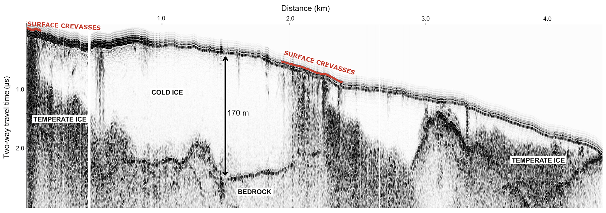
Figure 2The 30 MHz radar profile measured in 2015 along the red dashed line in Fig. 3a. This profile shows the presence of both cold ice (no reflection) and temperate ice (strong scattering).
The density profile and the surface elevation are updated only if F>Fref by adding the corresponding amount of snow at density ρ0.
The surface enthalpy field obtained using the distributed 1D model is used as a surface Dirichlet condition to solve the enthalpy equation in the 3D model. The 3D thermo-mechanical steady state of the glacier is then computed by following an iterative procedure:
Compute the steady-state enthalpy field from Eq. (7) with forced by the surface enthalpy field given by the distributed 1D model.
-
Compute Qlat from Eqs. (10) and (11).
-
Solve the ice velocity and deformational heat from the Stokes equation.
-
Compute the steady-state enthalpy field from Eq. (7) with Qlat determined in Step 2.
-
Steps 2, 3 and 4 are repeated until a steady state is reached.
Table 1Parameters of the surface model for enthalpy boundary conditions.
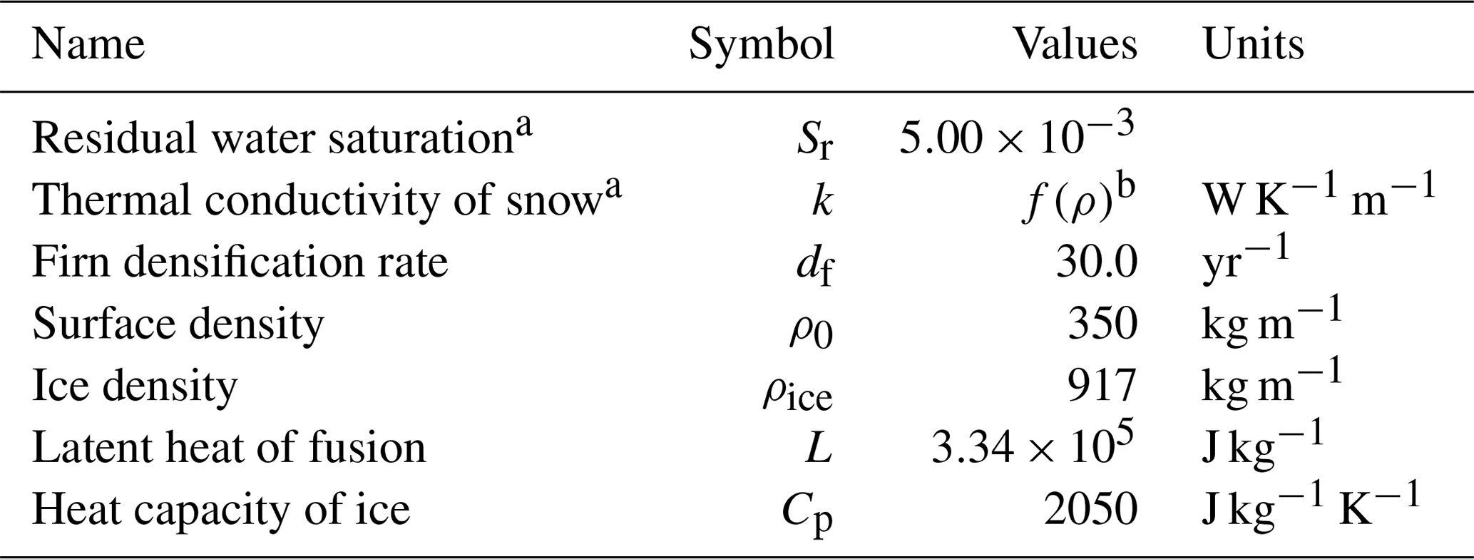
a Described in Gilbert et al. (2014b). b Formulation proposed by Calonne et al. (2011).
3.4.2 Bedrock topography and basal sliding condition
The main challenge in determining the glacier thermo-mechanical equilibrium is that (i) the bedrock topography is not known everywhere underneath the glacier, and (ii) the glacier is sliding, which means that a friction coefficient has to be quantified. In order to resolve these issues, we adopted the following steps.
-
Step 1. Starting from the measured surface topography in 2014, we run the coupled thermo-mechanical model with the interpolated bedrock topography and a uniform basal friction coefficient during a 10-year period forced by the steady-state surface mass balance and enthalpy. In order to obtain the steady-state mass balance, we shifted the temperature forcing (1980–2016 corrected reanalysis) by −0.7 ∘C, which allows us to obtain balanced mean conditions during the simulation period. The resulting mean surface mass balance is used as a steady mass balance associated with the 2014 glacier geometry. Here, we assume a uniform friction coefficient β (10−2 MPa a m−1) that allows the best match with the measured surface horizontal velocities.
-
Step 2. The computed changes in the free surface in Step 1 are reported to the bedrock topography by altering the bedrock by an amount equal to the free surface change (Gilbert et al., 2018).
-
Step 3. After a few iterations between Steps 1 and 2, we obtain a corrected bedrock topography where major flux divergences are avoided. Using this bedrock topography and the measured surface topography, we inverted for the friction coefficient β by constraining the surface velocity with emergence velocities, which are taken as opposite to surface mass balance. This is done by using a controlled inverse method to minimise a cost function defined from the misfit with measured surface velocities and a regularisation term (Gillet-Chaulet et al., 2012; Gagliardini et al., 2013). Following Gilbert et al. (2016, 2018) we define the cost function from the misfit between modelled and estimated emergence velocities;
-
Step 4. We finally run the model using the corrected bedrock topography and the inverted friction coefficient until the surface topography reaches a steady state.
3.5 Transient evolution
Transient simulations were performed at yearly time step using the steady-state glacier as the initial condition. Surface mass balance and enthalpy are updated each year from the surface model described previously and forced by daily temperature reanalysis. We assumed a constant basal friction parameter through time.
4.1 Thermal regime and ice thickness measured with the GPR
GPR data show that the Rikha Samba Glacier is a polythermal glacier consisting mainly of cold ice but with significant temperate areas (Figs. 2 and 3). The measured maximum thickness was 178±2 m in the middle part of the glacier where the surface slope is relatively gentle. Ice temperature measurements by the thermistor chain support the GPR interpretation of an upper cold ice layer with sub-zero temperatures at the depth of 10 m (annual mean −2 ∘C) in the ablation area of the glacier (Fig. 1). A notable characteristic of the GPR-based thermal regime is that the occurrence of temperate ice seems to be associated with the presence of surface crevasses (Figs. 2 and 3). The way that scattering is advected by the ice flow shows that the crevassed areas behave as a source term of scattering. It seems unlikely that the observed scattering would be produced by the crevasse field itself since the scatter occurs in the deeper part of the glacier where crevasses are not expected to persist. It would be rather more compatible with the formation of temperate ice which is then advected by ice flow.
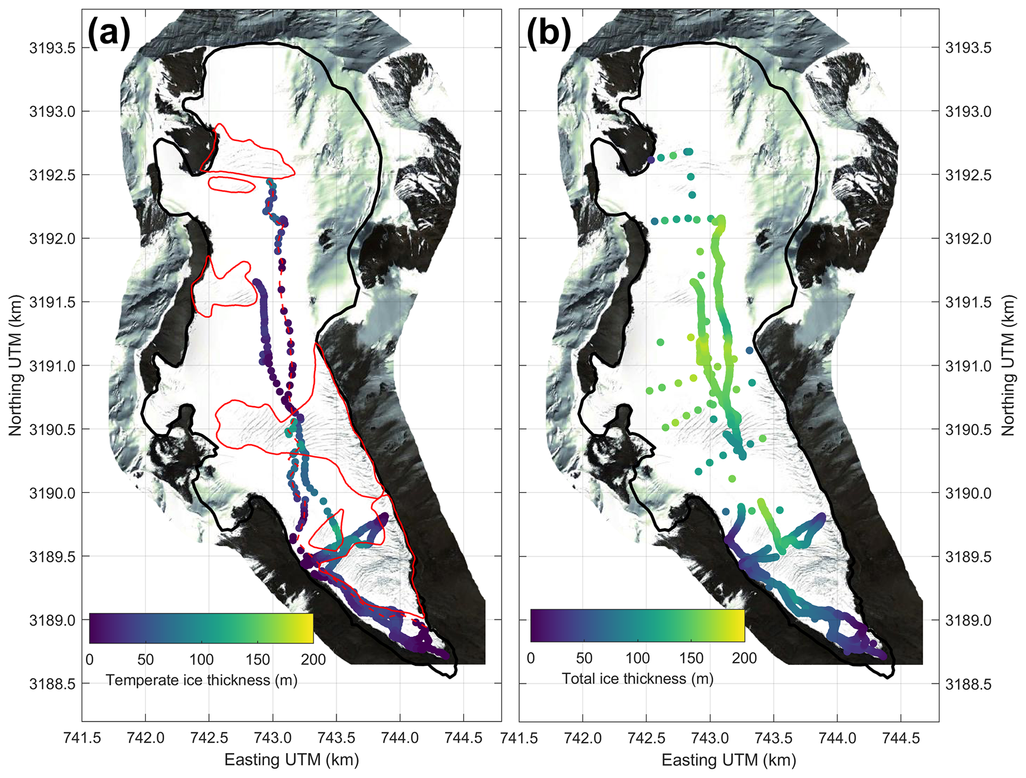
Figure 3(a) Measured temperate ice thickness (dots) and observed crevassed areas (red continuous lines). The red dashed line shows the location of the radar profile presented in Fig. 2. (b) Measured total ice thickness.
4.2 Surface mass balance
We run the mass balance model using the 2014 surface topography over the period 1980–2016 using calibrated temperature reanalysis data (ERA-Interim) (Dee et al., 2011) while assuming a constant precipitation rate. The parameters were constrained by the stake measurements in 2012/2013 (Gurung et al., 2016), meteorological observations (Gurung et al., 2016), and geodetic mass balance over the periods 1974–1994 and 1998–2010 (Fujita and Nuimura, 2011) (Fig. 4). The parameters are summarised in Table 2.
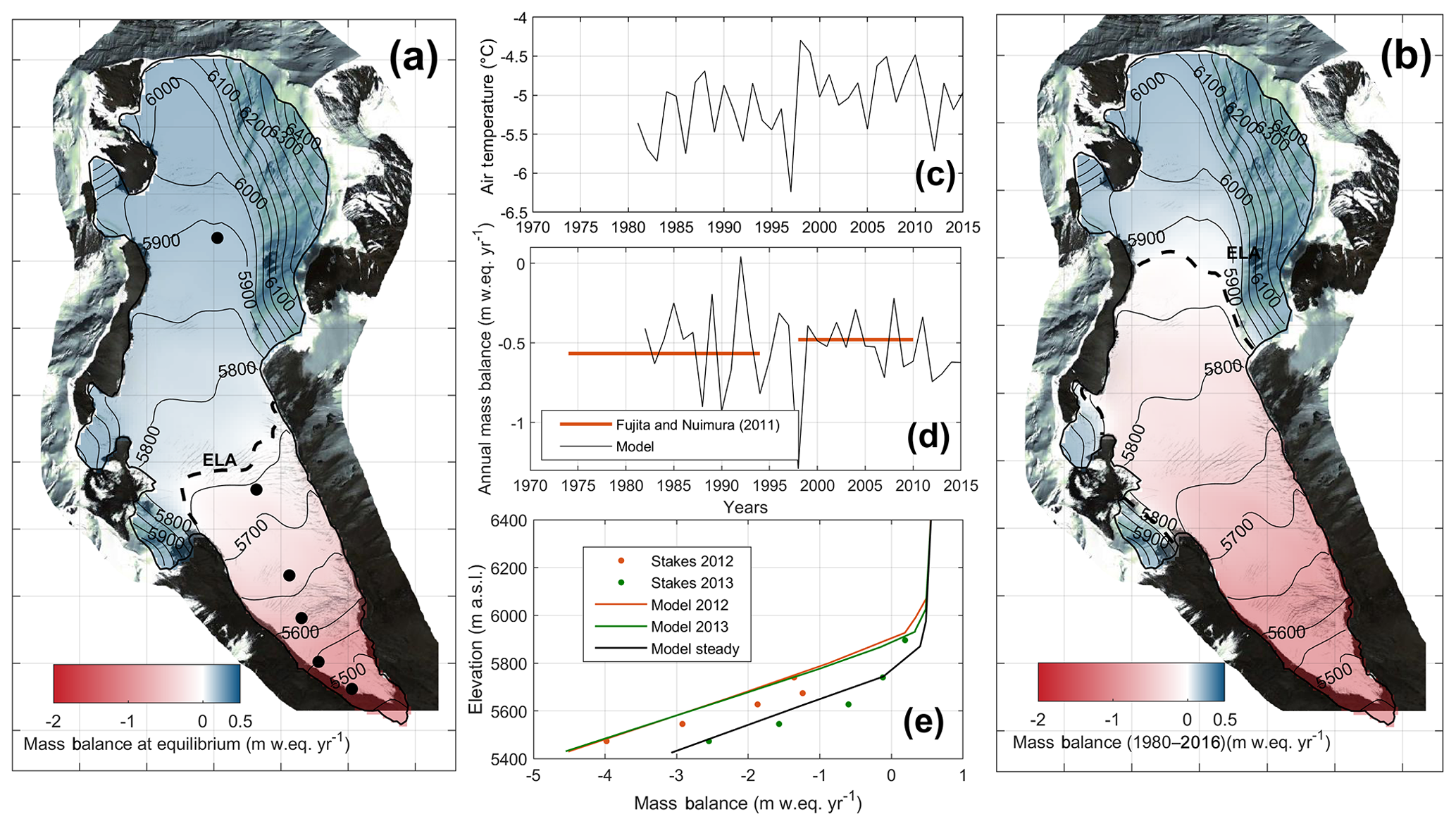
Figure 4Modelled mass balance using ERA-Interim reanalysis data. (a) Surface mass balance at equilibrium. Black dots are stake locations from Gurung et al. (2016). (b) Mean surface mass balance during the period 1980–2016. (c) Corrected ERA-Interim annual temperature (d) Modelled annual surface mass balance compared to geodetic data (Fujita and Nuimura, 2011). (e) Modelled surface mass balance as a function of elevation at equilibrium (black line), in 2012 (red line) and 2013 (green line). Dots are stake measurements for the years 2012 and 2013 (Gurung et al., 2016).
Table 2Parameters of the surface mass balance model.

a Gurung et al. (2016). b Calibrated in this study. c Fujita and Nuimura (2011). d Gilbert et al. (2016).
Balanced conditions for the 2014 geometry are reached for a climate that is 0.7 ∘C colder than the 1980–2016 climate with an equilibrium line altitude (ELA) of 5770 m a.s.l. (the 1980–2016 ELA is 5880 m a.s.l.; Fujita and Nuimura, 2011). This provides a mean surface mass balance and a melting rate to force the steady-state glacier simulation (Fig. 4a).
The model is in good agreement with the observations but is not able to reproduce the same mass balance distribution as observed in 2013 (Fig. 4b–d). Probably, the inter-annual variability of the mass balance produced with our mass balance model is probably not very well-represented since we assume a constant precipitation rate. Furthermore, the Rikha Samba Glacier is a summer-accumulation-type glacier in which precipitation events in summer can significantly affect the mass balance through albedo feedback (Fujita and Ageta, 2000; Fujita, 2008). However, the long-term trend and the mass balance gradient agree with the observations, which is satisfactory for the purposes of this study focusing on the thermal regime.
4.3 Enthalpy surface boundary condition
The modelled upper boundary condition field (Fig. 5) reveals a mainly cold surface condition with a temperate band between 5800 and 5900 m a.s.l. where both melting and firn thickness are sufficient to maintain temperate conditions. In the higher part of the accumulation area, the water percolation occurs only in the first 2 m due to the limited amount of meltwater resulting in cold temperature at 10 m depth (see Site 1 in Fig. 5), whereas lower down at Site 2, meltwater percolates deep enough to keep temperate conditions all year round at 10 m depth. In the ablation zone (Site 3), water percolation is limited to the seasonal snow thickness, resulting in a cold boundary condition.
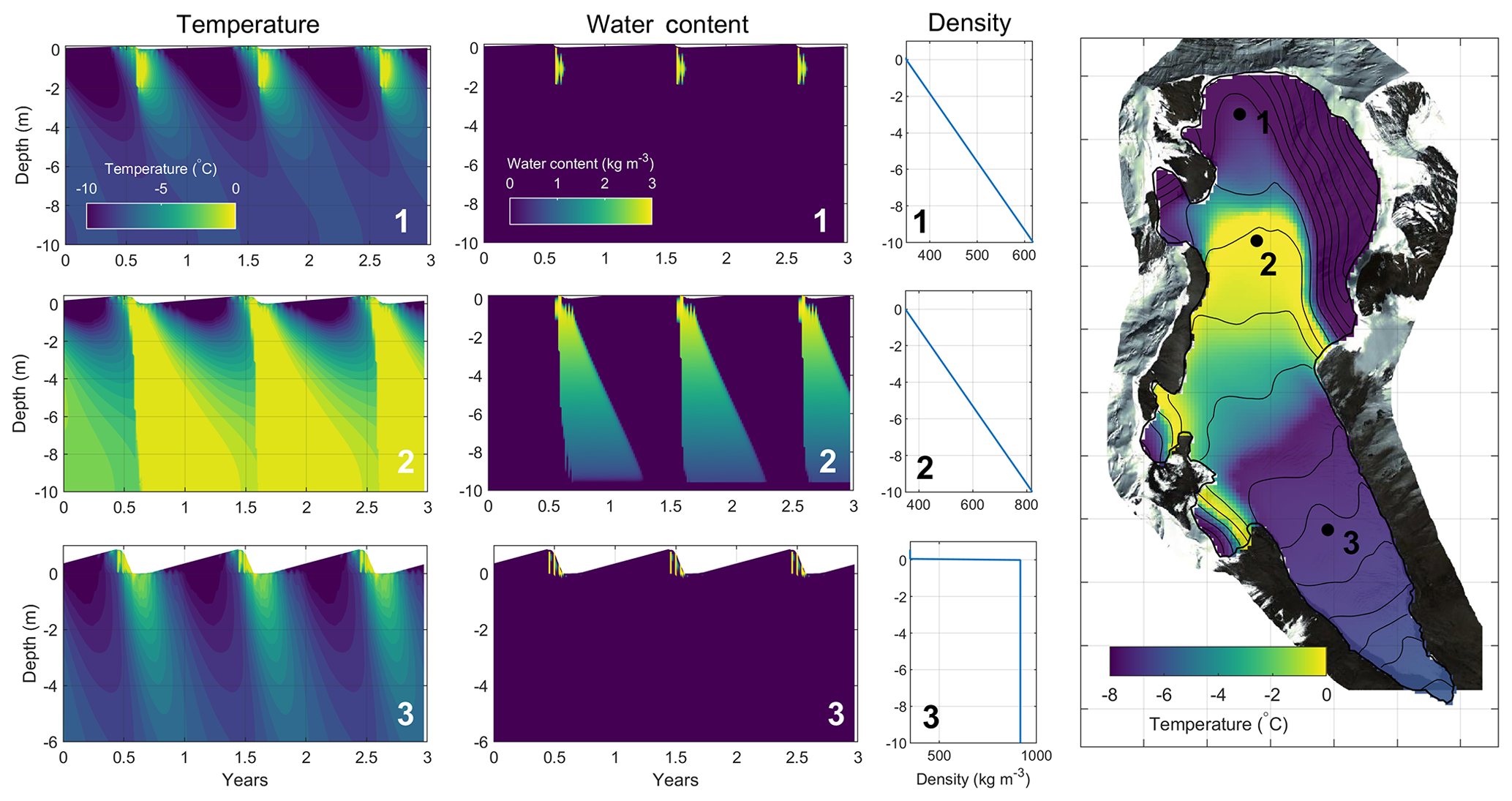
Figure 5One-dimensional temperature, water content and density modelled in the first 10 m of depth during 3 years and at three locations on the glacier. The one-dimensional model is forced by a reference temperature–precipitation annual cycle until reaching a stationary periodic response at 10 m depth. Mean annual temperature at 10 m depth is then used as an upper boundary condition for the thermo-mechanical model (mapped in the right panel).
4.4 Modelled steady-state glacier
The modelled steady-state glacier is in good accordance with measured ice thickness (Fig. 6) and measured horizontal velocities (Fig. 7a). We selected a value for the damage threshold of σth=0.05 MPa that allows the best match between observed and modelled crevassed areas (Fig. 7c). This value is within the recommended range found by Krug et al. (2014). The correction made on the bedrock topography following the method described in Sect. 3.4.2 greatly improves the quality of the modelling in areas without radar measurements (Fig. 6). A simple interpolation (Fig. 6a) would have led to non-physical ice thickness with unrealistic flux divergence, which is avoided by our method. The bedrock correction in place where there is radar measurement rarely exceeds 20 m (Fig. 6c) apart from a few exceptions (i.e. five points in the 2010 measurements). We preferred to allow the corrected bedrock to differ from radar measurement in order to favour the mass conservation associated with the prescribed surface mass balance. Moreover, radar measurements are uncertain, especially in temperate areas where the bedrock interface is weakly determined. The inversion of the basal friction coefficient (Fig. 7b) provides a final steady state where ice flow is in accordance with steady-state emergence velocities. The good agreement with horizontal velocities measured at stakes (Fig. 7a) shows that our estimated emergence velocities (from surface mass balance) are consistent with the observed ice flow.
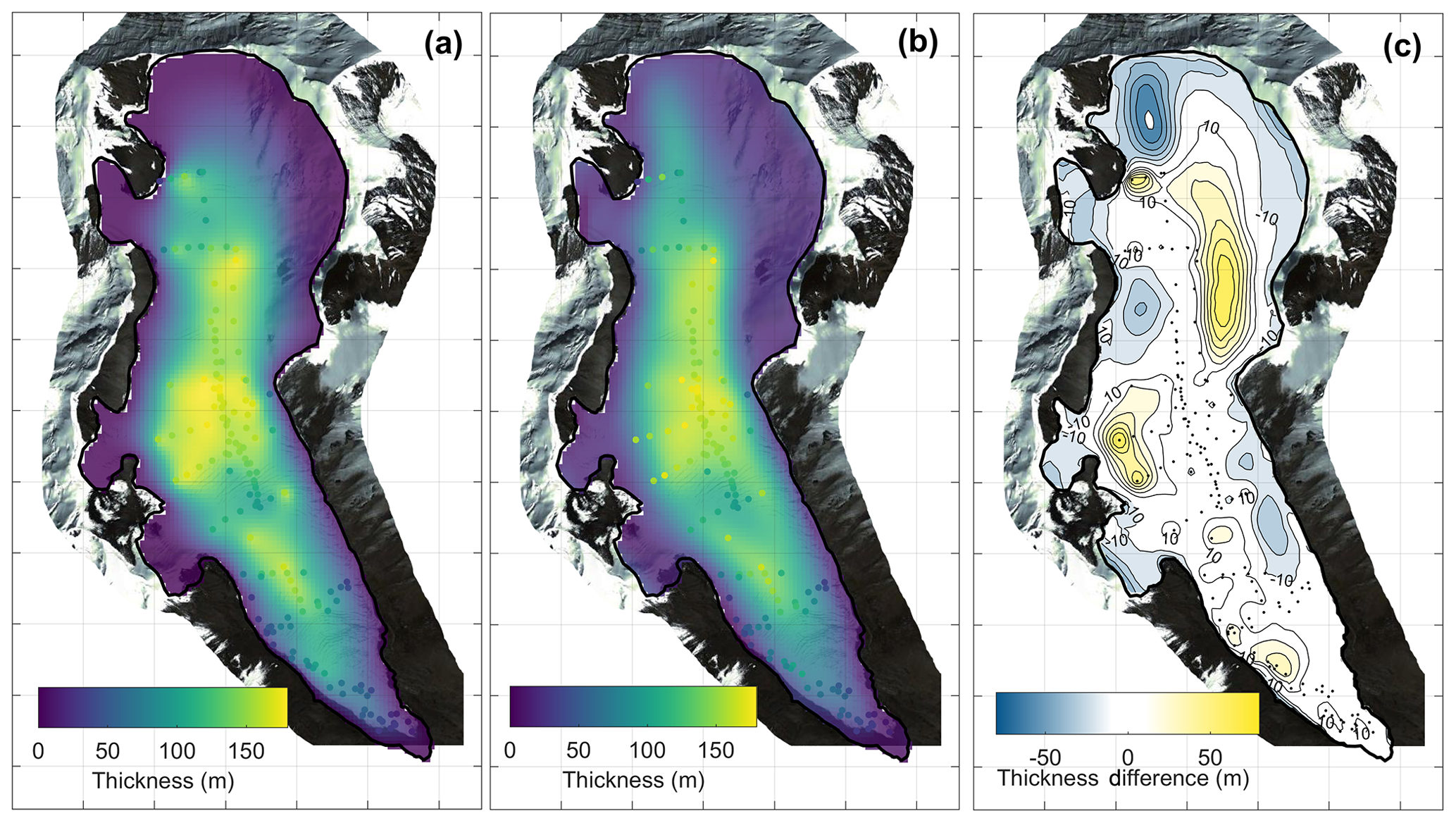
Figure 6(a) Interpolated ice thickness from GPR measurements (dots in the three panels). (b) Ice thickness after bedrock topography smoothing and correction using free surface relaxation. (c) Difference between interpolated and corrected ice thickness and positions of the GPR measurements (black dots).

Figure 7(a) Steady-state surface velocities compared with the measurements (coloured dots and inset). Contour lines are surface topography with 50 m intervals (b) Friction coefficient inferred from emergence velocities (assumed to be opposite of surface mass balance). Contour lines are bedrock topography with 50 m intervals. (c) Modelled crevassed areas from maximal Cauchy stress anomaly (colour scale) compared with observations (red lines).
4.5 Thermal regime: influence of meltwater percolation
Modelling results show that water percolation in crevasses strongly affects the steady-state thermal structure of the Rikha Samba Glacier, leading to large temperate zones even at the glacier bed (Figs. 8b and 9b). It significantly extends the temperate-based parts, which cover almost the entire ablation area. Although we adopted a simple approach for water percolation through crevasses, modelled temperate ice thickness is in fairly good agreement with the GPR data (Fig. 8b). If water percolation through crevasses is neglected, the thermal regime of the glacier forced by mainly cold upper boundary conditions (Fig. 5) would result in a mainly cold-based glacier (Fig. 9a). In such a case, cold ice advection from the higher part of the glacier is able to compensate for the temperate surface conditions of the lower accumulation zone (Fig. 5), and only two bands of temperate ice are able to reach the bed on both sides of the flow line of the glacier (Fig. 9a). Such a thermal regime is in disagreement with the observed amount of temperate ice from the GPR data (Fig. 8a). This indicates the significant role of deep water percolation through cracks in cold ice as suggested by the GPR observations. The observed (Figs. 8b and 9b) and modelled (Figs. 8c and 9c) crevassed area leads to a similar result, which validates our approach in modelling the location of the crevasses.
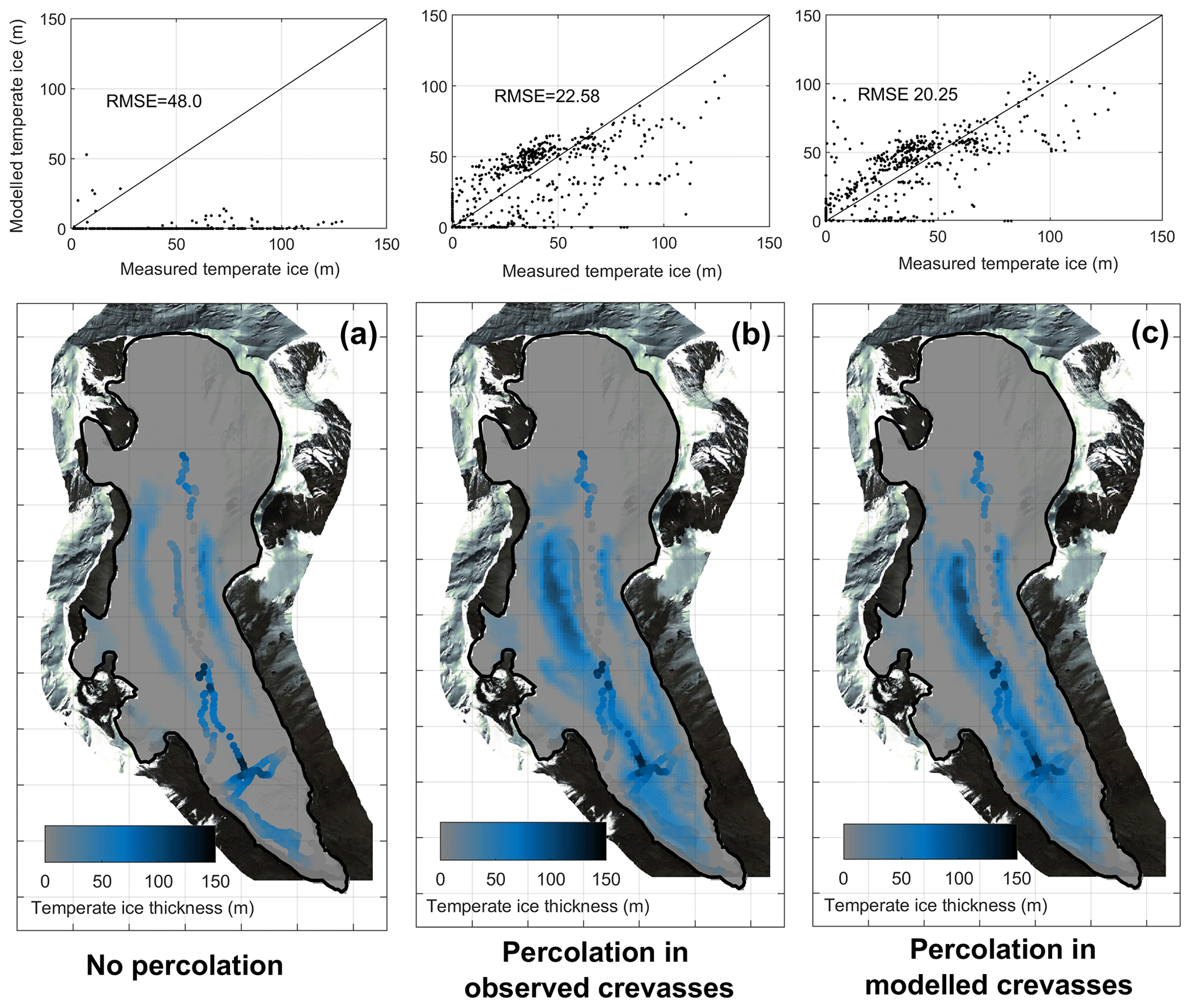
Figure 8Modelled vs. measured temperate ice thicknesses (upper panels) and comparison between model (colour background) and measurements (dots) (lower panels): (a) without crevasse influence, (b) with water percolation in observed crevassed areas and (c) with water percolation in modelled crevassed areas.
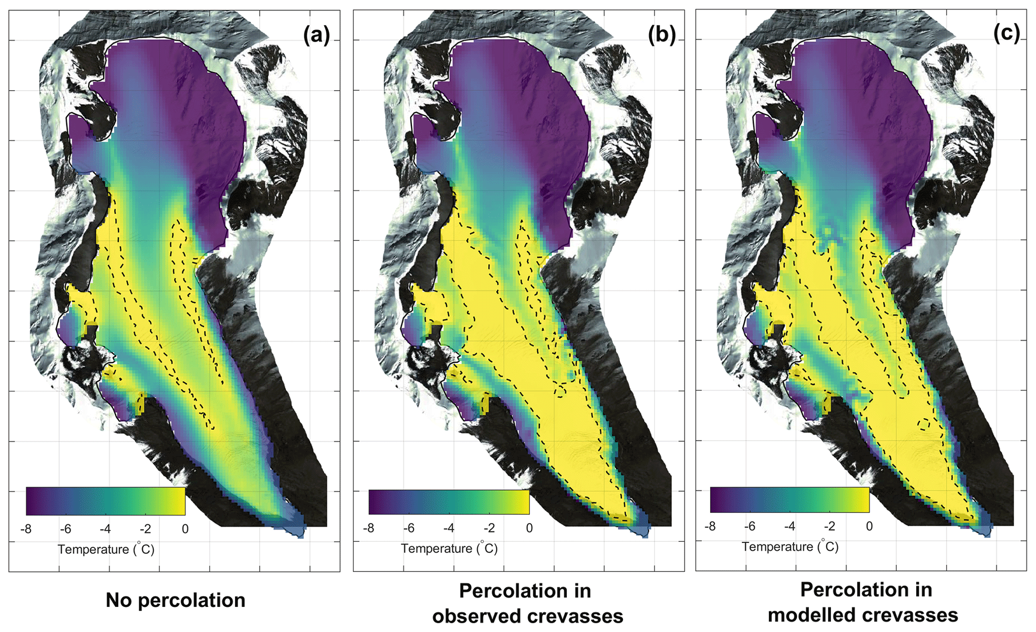
Figure 9Modelled steady-state basal temperature. (a) Without crevasse influence. (b) With water percolation in observed crevassed areas. (c) With water percolation in modelled crevassed areas. Dashed lines delimit the temperate areas.
4.6 Transient evolution
Despite the good agreement between the GPR data and the steady-state model, a significant difference exists at the highest crevassed field. A temperate area is clearly visible in the GPR data (Fig. 3a) whereas the steady-state thermal regime model predicts cold ice (Fig. 8). Mass balance measurements show that the Rikha Samba Glacier has not been in an equilibrium state for at least 40 years, with an almost constantly negative rate of −0.5 m w.e. a−1 (Fig. 4d). This temperate area could therefore be the signature of a transient response to air temperature warming. In order to investigate the potential impact of 40 years of unbalanced state on the glacier thermal regime, we performed a transient simulation starting in 1975 from the modelled steady state (with crevasse locations imposed from the modern observations showed in Fig. 3a) and forced by the ERA-Interim reanalysis time series (Fig. 4c). It shows that the upper boundary conditions changed significantly with a cooling of the former accumulation zone in response to firn disappearance and a warming of the highest elevation due to melting increase (Fig. 10b). After a 40-year run, a temperate zone, which do not exist at the steady state, had developed in the highest crevassed area (Fig. 10c–d) as observed in the 2015 GPR measurements (Fig. 10d). This result strongly suggests that the presence of temperate ice in this zone is a result of a transient response to the air temperature warming and increasing surface melting at the higher elevations. The results also agree better with the observations, including the thermistor data (Fig. 10a).
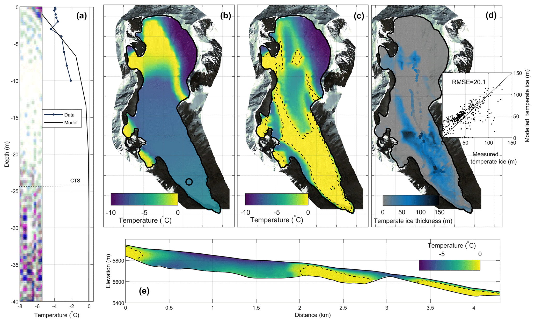
Figure 10Modelled thermal regime after a 40-year transient run forced by mean climatic condition over the period 1981–2016 (see Fig. 3b). (a) Modelled and measured mean temperature profile (2014/2015) in the ablation zone (black circle in b). The inset shows the radar measurement next to the thermistor (black circle in b) with the dashed line showing the modelled cold–temperate transition surface (CTS). (b) Mean surface boundary condition over the period 1981–2016. (c) Modelled basal temperature. (d) Distribution of modelled and measured temperate ice thickness. (e) Modelled temperature along the radar longitudinal section presented in Fig. 2.
To assess the sensitivity of the thermal regime to future temperature change, we performed a future simulation of the glacier retreat and thermal change until 2100 with (Fig. 11) and without (Fig. 12) water percolation through crevasses for a linearly increasing temperature of +1 ∘C between 2014 and 2100 (+1.7 ∘C in comparison with the steady-state climatic condition). This shows a much faster development of a new temperate area when water percolation in the crevasses is taken into account. In such a scenario, the glacier becomes almost entirely temperate-based by 2050 (Fig. 11), whereas it would have remained almost entirely cold had water percolation through the crevasses been neglected (Fig. 12). This highlights the crucial role of deep water percolation through cracks when modelling the past and future changes of glaciers' thermal regimes.
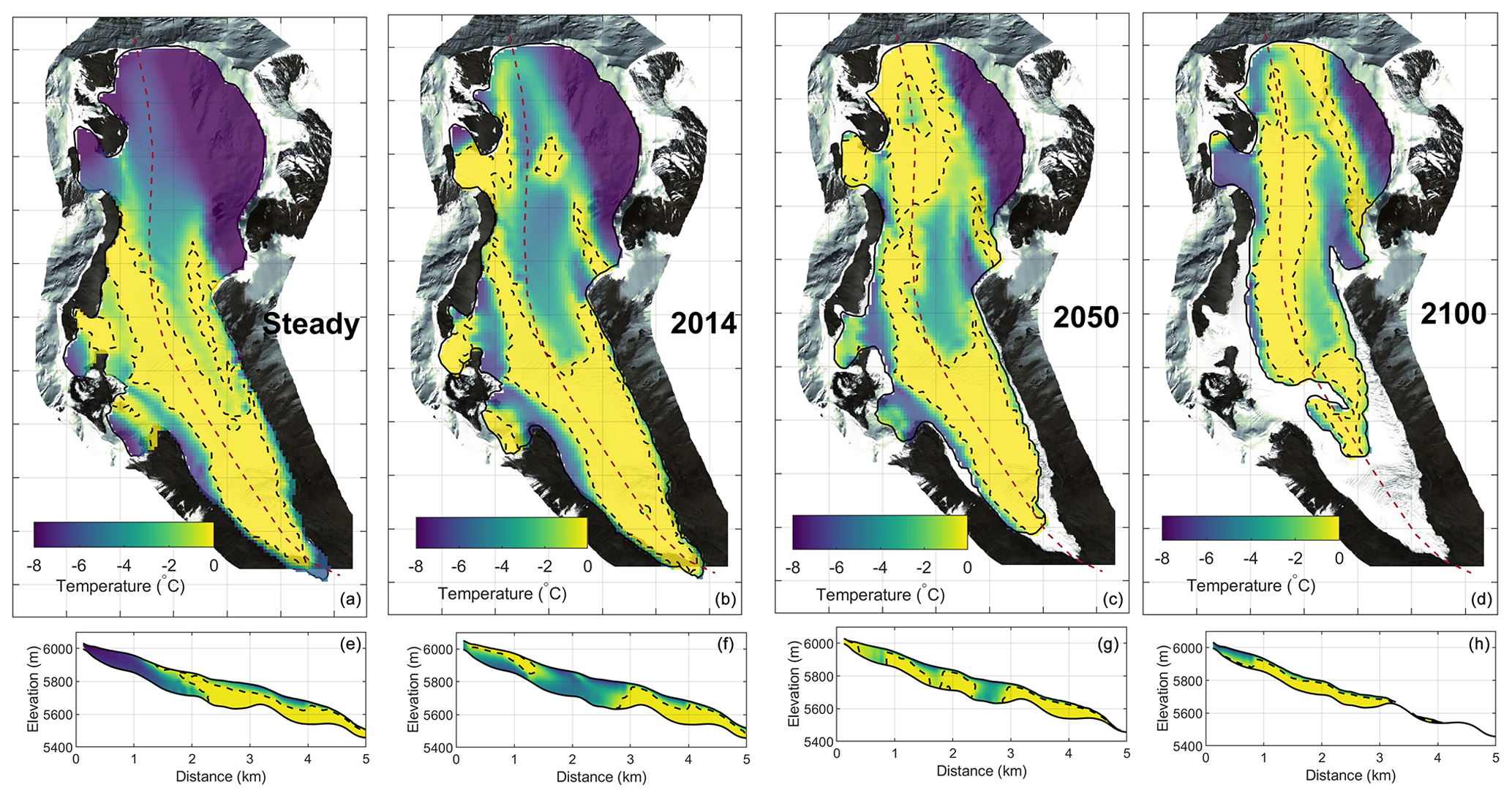
Figure 11Future evolution of Rikha Samba Glacier assuming a linear temperature increase of +1 ∘C between 2014 and 2100 (+1.7 ∘C in comparison with the steady-state climatic condition). Panels (a)–(d) represent basal temperature evolution. Panels (e)–(h) are temperature evolution along the middle longitudinal section. Black dashed lines delimit the cold–temperate transition surface.
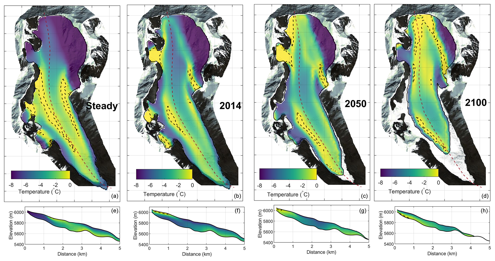
Figure 12Same as Fig. 11 but without water percolation in crevasses.
5.1 Uncertainty
The sensitivity experiment performed for the steady-state simulation shows that the amount of modelled basal temperate ice can vary significantly depending on the choice of parameters associated with firn thickness and basal heat flux, which are poorly constrained. However, the thickness of the modelled temperate ice always remains much less than indicated by the GPR observations if the crevasse influence is not taken into account. This means that uncertainty on those parameters alone does not explain the disagreement between data and model when the role of crevasses is neglected.
The mass balance model we used is simplified since we did not take into account the seasonality and time variation in precipitation, which can be sources of uncertainties in our study. However, the main focus of this study is the thermal regime of the glacier, and, hence, we do not claim that our simulation is accurate regarding the Rikha Samba Glacier past and future evolution. Our study relies on a long-term average of the surface mass balance and our simple calibrated model should be able to adequately capture it.
Since the density of ice is well-constrained and there was no snow or firn over the surveyed part of the glacier at the time of the field measurement in 2015, the main uncertainties of the GPR measurements arise from the GPS positioning of the GPR measurements, the radar wavelength and scattering of the radar signal. For the point measurements and those parts of the GPR profiles along which the bedrock reflection was clearly identified, the accuracy of the horizontal coordinates is about ±20 m, especially on the steepest surface slopes. In addition, the vertical resolution of the GPR signal is usually considered to be approximately one-quarter of the radar signal wavelength, which is about 5.6 and 33.6 m for the 30 and 5 MHz antennae, respectively. In other words, the vertical resolution of the englacial scattering, interpreted as temperate ice and ice thickness along the continuous GPR profiles, is about 1.4 m, whereas the same for the ice thickness obtained from the point measurements is about 8.4 m. The manual picking of bed reflectors in the radargrams introduces extra uncertainties up to 20 m, especially in temperate areas where the bed reflectors are weaker (see Fig. 2). Finally, the limited coverage of the radar profiles on the glacier introduces uncertainty in the bedrock topography inferred from the GPR data even after correction using the model. Uncertainties in the surface DEM are expected to be lower than 1 m and do not introduce extra uncertainties in the bedrock topography reconstructed from the measured thicknesses. Our interpretation of the thermal regime based on the englacial radar scattering of the GPR 30 MHz profiles is supported by previously found close agreement between the observed scattering and borehole temperatures without significant difference in observed englacial scattering relative to the expected measurement error at 10, 35 and 50 MHz antenna frequencies (Wilson et al., 2013).
In the modelled bedrock topography, the difficulty arises from the fact that the friction coefficient is unknown and we had to assume a uniform value of basal friction coefficient to correct the bedrock topography from flux divergence anomalies. The friction coefficient we inferred in a second step to force the steady emergence velocity to match the balanced surface mass balance is therefore affected by ice thickness errors. The resulting velocity field is consistent with the surface mass balance, but uncertainties in the respective contribution of the basal sliding and ice deformation to surface velocities remain. This makes the interpretation of the modelled basal friction difficult (Fig. 7b), which thus has to be seen more as a tuning parameter than a parameter revealing physical processes.
5.2 Role of surface runoff through supraglacial streams
Our study shows that the thermal regime of the Rikha Samba Glacier can be modelled by taking into account the liquid water derived from local surface melt percolating into crevassed fields. Neglect of water inputs coming from surface runoff through supraglacial streams seems thus to be a valid hypothesis. For a polythermal glacier with a cold surface layer, which is a common feature in the ablation areas where firn heating is nonexistent, surface runoff occurs in well-marked and persistent streams at the surface (Ryser et al., 2013). These streams bring water into the crevasse fields through a few localised entry points only. Hence, as there is only a relatively small contact surface between the streams and cold ice, a limited amount of water will refreeze. This is why the influence of surface runoff on the thermal regime of the glacier is likely to remain limited. Similarly, Lüthi et al. (2015) have concluded that moulins have little influence on the thermal regime of the Greenland Ice Sheet since they can be represented as line sources which provide limited warming to the surrounding ice. On the contrary, surface melting occurring in crevassed fields is well-distributed and can release latent heat on a much larger area, thus having a stronger impact on the thermal regime.
5.3 Enhanced influence of climate change on glaciers' thermal regime and dynamics
The influence of deep latent heat release through meltwater percolation in crevasses has been already inferred for Greenland. Lüthi et al. (2015) and Seguinot et al. (2020) observed temperature anomalies in borehole measurements that can only be explained by latent heat released down to a 400 m depth in crevassed fields. Similar conclusions have been made by Hills et al. (2017), although they show that these effects remain localised and may not really influence the thermal regime of the Greenland Ice Sheet on a large scale. In the case of mountain valley glaciers, crevassed fields can cover a significant fraction of the total glacier area, which is combined with a generally much faster ice flow, leading to efficient advective processes that transport the heat produced in the crevassed areas. The results of these combined effects are significant, greatly influencing the thermal regime at the glacier scale as shown in this study. As already pointed out for ice sheets (Phillips et al., 2010, 2013), the timescale of the glacier thermal regime response to climate change is also greatly diminished in comparison with the case where only heat diffusion and advection of surface changes are involved in the warming process. However, we show here that deep water percolation is likely restricted to the crevassed areas and absent elsewhere in order to model the observed thermal structure. This restricts the spatial extent of the process on the glacier as it is dependent on the bedrock topography and its related crevasse positions. For instance, the Yala Glacier, another polythermal glacier in the Nepal Himalaya (Sugiyama et al., 2013), is entirely cold in its ablation area, likely due to thinner ice and a lack of crevassed areas. Nevertheless, it is likely that the meltwater percolation via crevasses has a significant impact on the thermal regime of numerous polythermal high-altitude glaciers. Future warming could also lead to a faster thermal regime response than previously thought (Gilbert et al., 2015), especially in the cold accumulation areas where the pre-industrial melting rates were not sufficient to form temperate ice.
In this study, we use GPR measurements to show that the high-elevation Himalayan Rikha Samba Glacier is polythermal. We interpret the field observations of the temperate ice thickness using a 3D thermo-mechanical model constrained by a surface model taking into account water percolation in firn and seasonal snow. We show that the firn–snow heating, heat deformation and geothermal heat flux alone cannot explain the observed amount of temperate ice. The combined evidence of the model and observations reveals that valley-type mountain glaciers in cold climates are greatly affected by water percolation into crevassed fields which release latent heat into the ice body. This affects the thermal regime at the scale of the whole glacier, making temperate ice zones much larger than they would be without this effect. This enables sliding in large areas of the bed, largely affecting the glacier dynamics and thickness.
We also show that the thermal regime of the Rikha Samba Glacier is affected by a transient response to the last 40 years' air temperature warming, extending the temperate area to the highest part of the glacier. The thermal changes are occurring at a much smaller timescale (∼50 years) due to the crevasse effect compared to what it would be by advection–diffusion processes alone (>100 years). Our study reveals the crucial role of deep water percolation through cracks in determining both the steady-state and transient thermal structure of the polythermal glacier. We provide a simple approach easily applicable to any glaciers for a more accurate reconstruction of complex thermal structures such as the one observed in the case of the Rikha Samba Glacier.
As required by ICIMOD publication policy, GPR data used in this study will be made publicly available through ICIMOD's Regional Database System at http://rds.icimod.org (last access: 9 April 2020; ICIMOD, 2020). ICIMOD has an open data policy. The modelling code is based on the open-source code Elmer/Ice available at http://elmerfem.org/elmerice/wiki/doku.php (last access: 9 April 2020; Elmer/Ice, 2020). It includes an example based on the case presented in this paper.
AS and AG designed the study. AG performed the modelling analysis. AS, TRG and TCS conducted the fieldwork in 2015. KF and TF conducted the fieldwork in 2010. AS and TF analysed the GPR data. TRG and KF analysed the ERA-Interim data and mass balance. SBM analysed the DEM data. AG and AS wrote the paper with contributions from all other authors.
The authors declare that they have no conflict of interest.
We would like to thank Martin Lüthi and the one anonymous reviewer for their valuable comments that significantly improved the quality and readability of the manuscript. The authors would like to thank Laxmi Rai for his support in the field measurement campaign in 2015 and Jaana Gustafsson and Thomas Zwinger for their input when designing the study as well as the entire field teams in 2010, 2014 and 2015. The views and interpretations in this publication are those of the authors' and are not necessarily attributable to their respective organisations.
This work was supported by ICIMOD's Cryosphere Initiative, funded by Norway and by ICIMOD core funds contributed by the governments of Afghanistan, Australia, Austria, Bangladesh, Bhutan, China, India, Myanmar, Nepal, Norway, Pakistan, Sweden and Switzerland. Adrien Gilbert received funding from the University of Oslo “EarthFlows” initiative and funding from the European Research Council under the European Union's Seventh Framework Programme (FP/2007-2013)/ERC (grant no. 320816). Koji Fujita was supported by JSPS-KAKENHI (grant nos. 17H01621, 17H06104 and 18KK0098), and JSPS and SNSF under the Joint Research Projects (JRPs).
This paper was edited by Evgeny A. Podolskiy and reviewed by Martin Lüthi and one anonymous referee.
Aschwanden, A., Bueler, E., Khroulev, C., and Blatter, H.: An enthalpy formulation for glaciers and ice sheets, J. Glaciol., 58, 441–457, https://doi.org/10.3189/2012JoG11J088, 2012.
Bennett, M. M. and Glasser, N. F.: Glacial Geology: Ice Sheets and Landforms, John Wiley & Sons, Oxford, ISBN 978-0-470-51690-4, 2011.
Boon, S. and Sharp, M.: The role of hydrologically-driven ice fracture in drainage system evolution on an Arctic glacier, Geophys. Res. Lett., 30, 18, https://doi.org/10.1029/2003GL018034, 2003.
Calonne, N., Flin, F., Morin, S., Lesaffre, B., Rolland du Roscoat, S., and Geindreau, C.: Numerical and experimental investigations of the effective thermal conductivity of snow, Geophys. Res. Lett., 38, L23501, https://doi.org/10.1029/2011GL049234, 2011.
Cuffey, K. and Paterson, W. S. B.: The Physics of Glaciers, Elsevier, Butterworth-Heineman, Burlington, MA, USA, ISBN 9781493300761, 2010.
Dee, D. P., Uppala, S. M., Simmons, A. J., Berrisford, P., Poli, P., Kobayashi, S., Andrae, U., Balmaseda, M. A., Balsamo, G., Bauer, P., Bechtold, P., Beljaars, A. C. M., van de Berg, L., Bidlot, J., Bormann, N., Delsol, C., Dragani, R., Fuentes, M., Geer, A. J., Haimberger, L., Healy, S. B., Hersbach, H., Hólm, E. V., Isaksen, L., Kållberg, P., Köhler, M., Matricardi, M., McNally, A. P., Monge-Sanz, B. M., Morcrette, J.-J., Park, B.-K., Peubey, C., de Rosnay, P., Tavolato, C., Thépaut, J.-N., and Vitart, F.: The ERA-Interim reanalysis: configuration and performance of the data assimilation system, Q. J. Roy. Meteorol. Soc., 137, 553–597, https://doi.org/10.1002/qj.828, 2011.
Elmer/Ice: Elmer/Ice wiki, available at: http://elmerfem.org/elmerice/wiki/doku.php, last access: 9 April 2020.
Faillettaz, J., Sornette, D., and Funk, M.: Numerical modeling of a gravity-driven instability of a cold hanging glacier: reanalysis of the 1895 break-off of Altelsgletscher, Switzerland, J. Glaciol., 57, 817–831, https://doi.org/10.3189/002214311798043852, 2011.
Fischer, A.: Calculation of glacier volume from sparse ice-thickness data, applied to Schaufelferner, Austria, J. Glaciol., 55, 453–460, https://doi.org/10.3189/002214309788816740, 2009.
Fountain, A. G. and Walder, J. S.: Water flow through temperate glaciers, Rev. Geophys., 36, 299–328, https://https://doi.org/10.1029/97RG03579, 1998.
Fujita, K.: Effect of precipitation seasonality on climatic sensitivity of glacier mass balance, Earth Planet. Sci. Lett., 276, 14–19, https://doi.org/10.1016/j.epsl.2008.08.028, 2008.
Fujita, K. and Ageta, Y.: Effect of summer accumulation on glacier mass balance on the Tibetan Plateau revealed by mass-balance model, J. Glaciol., 46, 244–252, https://doi.org/10.3189/172756500781832945, 2000.
Fujita, K. and Nuimura, T.: Spatially heterogeneous wastage of Himalayan glaciers, P. Nat. Acad. Sci. USA, 108, 14011–14014, https://doi.org/10.1073/pnas.1106242108, 2011.
Fujita, K., Nakawo, M., Fujii, Y., and Paudyal, P.: Changes in glaciers in Hidden Valley, Mukut Himal, Nepal Himalayas, from 1974 to 1994, J. Glaciol., 43, 583–588, https://doi.org/10.3189/S002214300003519X, 1997.
Fujita, K., Nakazawa, F., and Rana, B.: Glaciological observations on Rikha Samba Glacier in Hidden Valley, Nepal Himalayas, 1998 and 1999, Bull. Glaciol. Res., 18, 31–35, 2001.
Gagliardini, O., Zwinger, T., Gillet-Chaulet, F., Durand, G., Favier, L., de Fleurian, B., Greve, R., Malinen, M., Martín, C., Råback, P., Ruokolainen, J., Sacchettini, M., Schäfer, M., Seddik, H., and Thies, J.: Capabilities and performance of Elmer/Ice, a new-generation ice sheet model, Geosci. Model Dev., 6, 1299–1318, https://doi.org/10.5194/gmd-6-1299-2013, 2013.
Gilbert, A., Vincent, C., Wagnon, P., Thibert, E., and Rabatel, A.: The influence of snow cover thickness on the thermal regime of Tête Rousse Glacier (Mont Blanc range, 3200 m asl): consequences for outburst flood hazards and glacier response to climate change, J. Geophys. Res., 117, F04018, https://doi.org/10.1029/2011JF002258, 2012.
Gilbert, A., Gagliardini, O., Vincent, C., and Wagnon, P.: A 3-D thermal regime model suitable for cold accumulation zones of polythermal mountain glaciers, J. Geophys. Res., 119, 1876–1893, https://doi.org/10.1002/2014JF003199, 2014a.
Gilbert, A., Vincent, C., Six, D., Wagnon, P., Piard, L., and Ginot, P.: Modeling near-surface firn temperature in a cold accumulation zone (Col du Dôme, French Alps): from a physical to a semi-parameterized approach, The Cryosphere, 8, 689–703, https://doi.org/10.5194/tc-8-689-2014, 2014b.
Gilbert, A., Vincent, C., Gagliardini, O., Krug, J., and Berthier, E.: Assessment of thermal change in cold avalanching glaciers in relation to climate warming, Geophys. Res. Lett., 42, 6382–6390, https://doi.org/10.1002/2015GL064838, 2015.
Gilbert, A., Flowers, G. E., Miller, G. H., Rabus, B. T., Van Wychen, W., Gardner, A. S., and Copland, L.: Sensitivity of Barnes Ice Cap, Baffin Island, Canada, to climate state and internal dynamics, J. Geophys. Res., 121, 1516–1539, https://doi.org/10.1002/2016JF003839, 2016.
Gilbert, A., Leinss, S., Kargel, J., Kääb, A., Gascoin, S., Leonard, G., Berthier, E., Karki, A., and Yao, T.: Mechanisms leading to the 2016 giant twin glacier collapses, Aru Range, Tibet, The Cryosphere, 12, 2883–2900, https://doi.org/10.5194/tc-12-2883-2018, 2018.
Gillet-Chaulet, F., Gagliardini, O., Seddik, H., Nodet, M., Durand, G., Ritz, C., Zwinger, T., Greve, R., and Vaughan, D. G.: Greenland ice sheet contribution to sea-level rise from a new-generation ice-sheet model, The Cryosphere, 6, 1561–1576, https://doi.org/10.5194/tc-6-1561-2012, 2012.
Gurung, S., Bhattarai, B. C., Kayastha, R. B., Stumm, D., Joshi, S. P., and Mool, P. K.: Study of annual mass balance (2011–2013) of Rikha Samba Glacier, Hidden Valley, Mustang, Nepal, Sci. Cold Arid Reg., 8, 311–318, 2016.
Gusmeroli, A., Jansson, P., Pettersson, R., and Murray, T.: Twenty years of cold layer thinning at Storglaciaren, sub–Arctic Sweden, 1989–2009, J. Glaciol., 58, 3–10, https://https://doi.org/10.3189/2012JoG11J018, 2012.
Hills, B. H., Harper, J. T., Humphrey, N. F., and Meierbachtol, T. W.: Measured horizontal temperature gradients constrain heat transfer mechanisms in Greenland ice, Geophys. Res. Lett., 44, 9778–9785, https://https://doi.org/10.1002/2017GL074917, 2017.
ICIMOD: Regional Database System, a non-stop data portal for the Hindu Kush Himalaya, available at: http://rds.icimod.org, last access: 9 April 2020.
Irvine-Fynn, T. D. L., Moorman, B. J., Williams, J. L. M., and Walter, F. S. A.: Seasonal changes in ground penetrating radar signature observed at a polythermal glacier, Bylot Island, Canada, Earth Surf. Process. Landform., 31, 892–909, https://doi.org/10.1002/esp.1299, 2006.
Krug, J., Weiss, J., Gagliardini, O., and Durand, G.: Combining damage and fracture mechanics to model calving, The Cryosphere, 8, 2101–2117, https://doi.org/10.5194/tc-8-2101-2014, 2014.
Liu, Y., Hou, S., Wang, Y., and Song, L.: Distribution of borehole temperature at four high altitude alpine glaciers in central Asia, J. Mt. Sci., 6, 221–227, https://doi.org/10.1007/s11629-009-0254-9, 2009.
Lüthi, M. P., Ryser, C., Andrews, L. C., Catania, G. A., Funk, M., Hawley, R. L., Hoffman, M. J., and Neumann, T. A.: Heat sources within the Greenland Ice Sheet: dissipation, temperate paleo-firn and cryo-hydrologic warming, The Cryosphere, 9, 245–253, https://doi.org/10.5194/tc-9-245-2015, 2015.
Mae, S.: Ice temperature of Khumbu Glacier, Seppyo, J. Jpn. Soc. Snow Ice, 38, Special Issue, 37–38, 1976.
Matheron, G.: Principles of geostatistics, Eco. Geol., 58, 1246–1266, https://https://doi.org/10.2113/gsecongeo.58.8.1246, 1963.
Miles, K. E., Hubbard, B., Quincey, D. J., Miles, E. S., Sherpa, T. C., Rowan, A. V., and Doyle, S. H.: Polythermal structure of a Himalayan debris-covered glacier revealed by borehole thermometry, Sci. Rep., 8, 16825, https://doi.org/10.1038/s41598-018-34327-5, 2018.
Miller, J. D., Immerzeel, W. W., and Rees, G.: Climate change impacts on glacier hydrology and river discharge in the Hindu Kush–Himalayas, Mt. Res. Dev., 32, 461–467, https://doi.org/10.1659/MRD-JOURNAL-D-12-00027.1, 2012.
Pellicciotti, F., Brock, B., Strasser, U., Burlando, P., Funk, M., and Corripio, J.: An enhanced temperature-index glacier melt model including the shortwave radiation balance: development and testing for Haut Glacier d'Arolla, Switzerland, J. Glaciol., 51, 573–587, https://https://doi.org/10.3189/172756505781829124, 2005.
Pettersson, R., Jansson, P., Huwald, H., and Blatter, H.: Spatial pattern and stability of the cold surface layer of Storglaciaren, Sweden, J. Glaciol., 53, 99–109, https://doi.org/10.3189/172756507781833974, 2007.
Phillips, T., Rajaram, H., and Steffen, K.: Cryo-hydrologic warming: a potential mechanism for rapid thermal response of ice sheets, Geophys. Res. Lett., 37, L20503, https://doi.org/10.1029/2010GL044397, 2010.
Phillips, T., Rajaram, H., Colgan, W., Steffen, K., and Abdalati, W.: Evaluation of cryo-hydrologic warming as an explanation for increased ice velocities in the wet snow zone, Sermeq Avannarleq, West Greenland, J. Geophys. Res., 118, 1241–1256, https://doi.org/10.1002/jgrf.20079, 2013.
Pralong, A. and Funk, M.: Dynamic damage model of crevasse opening and application to glacier calving, J. Geophys. Res., 110, B01309, https://doi.org/10.1029/2004JB003104, 2005.
Robin, G. D. Q.: Velocity of radio waves in ice by means of a bore-hole interferometric technique, J. Glaciol., 15, 151–159, https://https://doi.org/10.3189/S0022143000034341, 1975.
Ryser, C., Lüthi, M., Blindow, N., Suckro, S., Funk, M., and Bauder, A.: Cold ice in the ablation zone: its relation to glacier hydrology and ice water content, J. Geophys. Res., 118, 693–705, https://doi.org/10.1029/2012JF002526, 2013.
Seguinot, J., Funk, M., Bauder, A., Wyder, T., Senn, C., and Sugiyama, S.: Englacial warming indicates deep crevassing in Bowdoin Glacier, Greenland, Front. Earth Sci., 8, 65, https://doi.org/10.3389/feart.2020.00065, 2020.
Sugiyama, S., Fukui, K., Fujita, K., Tone, K., and Yamaguchi, S.: Changes in ice thickness and flow velocity of Yala Glacier, Langtang Himal, Nepal, from 1982 to 2009, Ann. Glaciol., 54, 157–162, https://https://doi.org/10.3189/2013AoG64A111, 2013.
Tao, W. and Shen, Z.: Heat flow distribution in Chinese continent and its adjacent areas, Prog. Nat. Sci., 18, 843–849, https://https://doi.org/10.1016/j.pnsc.2008.01.018, 2008.
Van der Veen, C. J.: Fracture propagation as means of rapidly transferring surface meltwater to the base of glaciers, Geophys. Res. Lett., 34, L01501, https://https://doi.org/10.1029/2006GL028385, 2007.
Wang, Y., Zhang, T., Ren, J., Qin, X., Liu, Y., Sun, W., Chen, J., Ding, M., Du, W., and Qin, D.: An investigation of the thermomechanical features of Laohugou Glacier No. 12 on Qilian Shan, western China, using a two-dimensional first-order flow-band ice flow model, The Cryosphere, 12, 851–866, https://doi.org/10.5194/tc-12-851-2018, 2018.
Watanabe, O., Takenaka, S., Iida, H., Kamiyama, K., Thapa, K. B., and Mulmi, D. D.: First results from Himalayan glacier boring project in 1981–1982, Part I. Stratigraphic analyses of full-depth cores from Yala Glacier, Langtang Himal, Nepal. Bull. Glacier Res., 2, 7–23, 1984.
Wilson, N. J., Flowers, G. E., and Mingo, L.: Comparison of thermal structure and evolution between neighboring subarctic glaciers, J. Geophys. Res., 118, 1443–1459, https://doi.org/10.1002/jgrf.20096, 2013.
Zhang, T., Xiao, C., Colgan, W., Qin, X., Du, W., Sun, W., Liu, Y., and Ding, M.: Observed and modelled ice temperature and velocity along the main flowline of East Rongbuk Glacier, Qomolangma (Mount Everest), Himalaya, J. Glaciol., 59, 438–448, https://https://doi.org/10.3189/2013JoG12J202, 2013.