Permafrost distribution and conditions at the headwalls of two receding glaciers (Schladming and Hallstatt glaciers) in the Dachstein Massif, Northern Calcareous Alps, Austria

Permafrost distribution in rock walls surrounding receding glaciers is an important factor in rock stability and rock wall retreat. We investigated bedrock permafrost distribution in the Dachstein Massif, Austria, reaching up to 2995 m a.s.l. The occurrence, thickness and thermal regime of permafrost at this partly glaciated mountain massif are scarcely known. We applied a multi-method approach with continuous ground surface and near-surface temperature monitoring (GST), measurement of the bottom temperature of the winter snow cover (BTS), electrical resistivity tomography (ERT), airborne photogrammetry, topographic maps, visual observations, and field mapping. Our research focused on several steep rock walls consisting of massive limestone above receding glaciers exposed to different slope aspects at elevations between ca. 2600 and 2700 m a.s.l. We aimed to quantify the distribution and conditions of bedrock permafrost particularly at the transition zone between the present glacier surface and the adjacent rock walls.

According to our ground temperature data, permafrost is mainly found at north-facing rock walls. At south-east-facing rock walls, permafrost is probable only in very favourable cold conditions at radiation-sheltered higher elevations (>2700 m a.s.l.). ERT measurements reveal high resistivities (>30 000 Ω m) at ≥1.5 m depth at north-exposed slopes (highest values >100 kΩ m). Deducted from laboratory studies and additional small-scale ERT measurements, these values indicate permafrost existence. Permafrost bodies were found at several rock walls independent of investigated slope orientation; however, particularly large permafrost bodies were found at north-exposed sites. Furthermore, at vertical survey lines, a pronounced imprint of the former Little Ice Age (LIA) ice margin was detected. Resistivities above and below the LIA line are markedly different. At the LIA glacier surface, the highest resistivities and lowest active-layer thicknesses were observed. The active-layer thickness increases downslope from this zone. Permafrost below the LIA line could be due to permafrost aggradation or degradation; however, the spatial patterns of frozen rock point to permafrost aggradation following glacier surface lowering or retreat. This finding is significant for permafrost and cirque erosion studies in terms of frost-influence weathering in similar high-mountain settings.

1 Introduction

Climate change has a great impact on perennially frozen and glaciated high-mountain regions (Haeberli and Hoelzle, 1995; Haeberli et al., 1997; Harris et al., 2001; Lieb et al., 2012). Glacier retreat (Paul et al., 2004; Zemp et al., 2008; Kellerer-Pirklbauer et al., 2008) is the visible evidence with a loss of an estimated 50 % of the original glacier volume in the European Alps between the end of the Little Ice Age around 1850 and 1975, a 10 % loss in 1975–2000, and a further 10 % in 2000–2009 (Haeberli et al., 2007, 2013; Magnin et al., 2017).

Invisible but also measurable are permafrost changes in the subsurface. Formerly glacier-covered rock surfaces with former temperatures around the melting point – conditioned by temperate glacier ice – become subjected to direct local atmospheric conditions after the ice melted. Depending on the slope orientation and shading effects of these rock surfaces, permafrost aggradation is possible at such sites after exposure. However, in the case of cold and polythermal glaciers (with cold ice restricted to cold, high-altitude parts of the glacier; Benn and Evans, 2010) permafrost might exist even below glacier-covered areas. In addition to that, glaciers might be separated from the adjacent headwall by a distinct gap or crevasse (randkluft). Such crevasses are also typical glacial features in our study area. Air can enter into this crevasse allowing for a better coupling of the air and bedrock even below the glacier surfaces and also more efficient cooling during the summer season (Sanders et al., 2012). Therefore, both a polythermal glacier and a glacier with a distinct randkluft might allow for permafrost aggregation below the glacier surface.

Changes in ground thermal conditions, permafrost extent and hydrology are all sensitive to predicted future climate change (Gobiet et al., 2014). A warming of about 0.5 to 0.8 ^∘C in the upper tens of metres of alpine permafrost between 2600 and 3400 m a.s.l. at the European Alps in the last century (Harris et al., 2003) results in a vertical mean rise of the lower limit of permafrost by about 1 m yr⁻¹ (Frauenfelder, 2005). Magnin et al. (2017) simulated the long-term temperature evolution at three rock wall sites between 3160 and 4300 m a.s.l. in the Mont Blanc massif from Little Ice Age (LIA) conditions to 2100 and concluded that permafrost degradation has been progressing since the LIA. This ongoing degradation can potentially trigger rock wall instabilities (Wegmann et al., 1998; Sattler et al., 2011; Ravanel and Deline, 2011; Kellerer-Pirklbauer et al., 2012; Krautblatter et al., 2013; Draebing et al., 2017a, b). Therefore, acquiring knowledge on the permafrost distribution and freezing and thawing in the active layer (Supper et al., 2014) is important in high-mountain areas particularly if infrastructure is potentially threatened (Kern et al., 2012). While ground surface temperature measurements in rock walls (e.g. Matsuoka and Sakai, 1999; Gruber et al., 2003; Kellerer-Pirklbauer, 2017) can provide valuable point information on rock temperature and thermal conditions of permafrost, geophysical techniques enable the visualisation of subsurface permafrost characteristics in 2D or 3D arrays. Several authors have used electrical resistivity tomography (ERT) for permafrost investigations in sediments (e.g. Kneisel et al., 2008; Hauck, 2001; Hauck et al., 2003; Marescot et al., 2003; Laxton and Coates, 2011; Rödder and Kneisel, 2012; Stiegler et al., 2014). In contrast, in rock walls comparable measurements are relatively scarce (e.g. Krautblatter and Hauck, 2007; Hartmeyer et al., 2012; Magnin et al., 2015; Draebing et al., 2017a, b), and for rock walls close above the present glacier surfaces (Supper et al., 2014), ERT data are widely missing. Accordingly, the aims of this study are to detect, delimit and characterise permafrost in the recently deglaciated rock walls surrounding the two retreating Schladming and Hallstatt glaciers in the Dachstein area and, thus, to contribute to the question of how widespread glacier retreat will affect permafrost degradation and/or aggradation in a mid-latitude mountain region.

2 Study area

2.1 General setting

The Dachstein Massif, with its highest peak the Hoher Dachstein (2995 m a.s.l.) located at $\mathrm{47}{}^{\circ }{\mathrm{28}}^{\prime }{\mathrm{32}}^{\prime \prime }$ N, ${\mathrm{13}}^{\circ }{\mathrm{36}}^{\prime }{\mathrm{23}}^{\prime \prime }$ E, is a mountain range in the Northern Calcareous Alps in Austria covering an area of about 400 km² (Fig. 1). The study area is characterised by steep rock walls (e.g. the Dachstein south wall with an 850 m altitude difference within a vertical distance of some hundred metres) towering above relatively flat, glacier-covered plateaus and extensive touristic infrastructure with cable cars, ski lifts and ski runs. In particular the Schladming Glacier (Fig. 1) is intensively used for alpine skiing. The surrounding headwalls are also partly used by means of a military transmitting station, lift stations and public climbing routes.

The prevailing rock type in the study area is the very compact Dachstein limestone (GBA, 1982; Gasser et al., 2009). The climatic conditions of the study area are dominated by west and north-east airflows. The main maximum of precipitation is during summer with a secondary maximum in winter. Air temperature measurements at the surface of the Schladming Glacier next to the Hunerkogel at 2600 m a.s.l. showed annual average temperatures (MAATs) of −2.4 ^∘C in the period 2007–2016.

This MAAT value at the Dachstein Massif indicates the presence of discontinuous permafrost in the study area (Humlum, 1998). The first evidence of the existence of permafrost in the study area was provided by measurements of the bottom temperature of the winter snow cover (BTS) carried out by Schopper (1989) and Lieb and Schopper (1991) in the proglacial area of the Schladming Glacier at 2300–2400 m a.s.l. According to these authors, the lower limit of discontinuous permafrost can be expected at this elevation. More recent simulations regarding the probability of permafrost existence in Austria (Ebohon and Schrott, 2009) or in the entire European Alps (Boeckli et al., 2012a, b) revealed that permafrost existence in the study area is particularly likely at north-exposed, higher-elevated slopes as well as in the proglacial area of the Schladming Glacier.

Our research focused on the lower parts of steep rock walls of recently deglaciated areas at four different measurement sites (MSs) at elevations between 2600 and 2700 m a.s.l. next to the Schladming and Hallstatt glaciers (Fig. 1). The Koppenkarstein site (MS-K; summit elevation 2863 m a.s.l.) was chosen due to the high probability of permafrost at this radiation-sheltered position; the pronounced randkluft; and the well-documented, high rates of glacier surface lowering since the LIA maximum around 1850. The Dirndln site (MS-D) was selected because of a distinct blowout depression between the glacier and the mountain (Fig. 2). This causes snow-poor and ice-free conditions at the foot slope of the mountain which probably reduced ice coverage even during the LIA extent of the glacier. The Gjaidstein site (MS-G) is slightly lower and oriented to the west which makes permafrost occurrence less probable. The cable car station is located at Hunerkogel (MS-H) which makes this site interesting in terms of endangered infrastructure. There are no sites oriented to the south as there is only a very small glacier facing south and the probability of permafrost at this site is much lower.

Figure 1 Location of the study area Dachstein Massif in Austria, and an overview map depicting the four different measurement sites within the study area. Glacier recession between ca. 1850 (LIA maximum) and 2012 is indicated. Abbreviations: MS-D, measurement site Dirndln; MS-G, measurement site Gjaidstein; MS-H, measurement site Hunerkogel; MS-K, measurement site Koppenkarstein. Orthophoto in the background by the province of Upper Austria, 2013.

2.2 Reconstruction of deglaciation

The Hallstatt Glacier and the Schladming Glacier have been subject to substantial mass loss and glacier surface lowering since the Little Ice Age (LIA; ca. 1850) and particularly in the last few decades. The Hallstatt Glacier lost about 50 % of its area and 52 % of its length, whereas the Schladming Glacier had reduced by 55 % in area and 48 % in length from the end of the LIA up until 2012. The retreat of the glaciers located at the Dachstein Massif since the LIA are well documented by Simony (1895), Moser (1997), Krobath and Lieb (2004), Helfricht (2009) or Fischer et al. (2015). New ice-free areas in the glacier forefield and the surrounding headwalls have afforded new touristic concepts and safety precautions over the years. A distinct randkluft exists at several places in the study area (see Fig. 1) and is commonly visible during the ablation season. The total length of the mapped randkluft in the area depicted in Fig. 1 was 2840 m in 2013 which was about 14.9 % of the total glacier boundary in this year.

In addition to the above-mentioned published glacier reconstructions, airborne photogrammetry, topographic maps, visual observations and field mapping were applied for the reconstruction of deglaciation at our sites. To visualise the vertical changes in the glacier surface, digital terrain models (DTMs) with a spatial resolution of 5 m were produced from published 1:25 000 maps of the German–Austrian Alpine Club from 1915 and the German–Austrian Alpine clubs from 2002 by digitising the 10 m contour lines and generating DTMs using the ArcGIS Topo-to-Raster function. The difference between both models showed the glacier retreat of 1915 to 2002. In addition, recent orthophotos from 2009 (provided by the federal government of Upper Austria) and data from the third Austrian glacier inventory (Fischer et al., 2015) enabled the mapping of the present glacier surface and, thus, the estimation of glacier retreat from 1915 to 2009. The comparison of historic photographs from 1958 (Schneider, July 1958, from Österreichischer Alpenverein, 1958) and our own photographs from 2013 to 2015 gave further information about the vertical surface lowering (Fig. 2).

Figure 2 Comparison of the glacier surface at the foot of the Koppenkarstein in 2013 (photo by Gitschthaler, 2 August 2013) and 1958 (photo by Schneider, July 1958, from Österreichischer Alpenverein, 1958). Note the obvious surface change at Hunerkogel. Note that the shooting location of both years is not exactly the same.

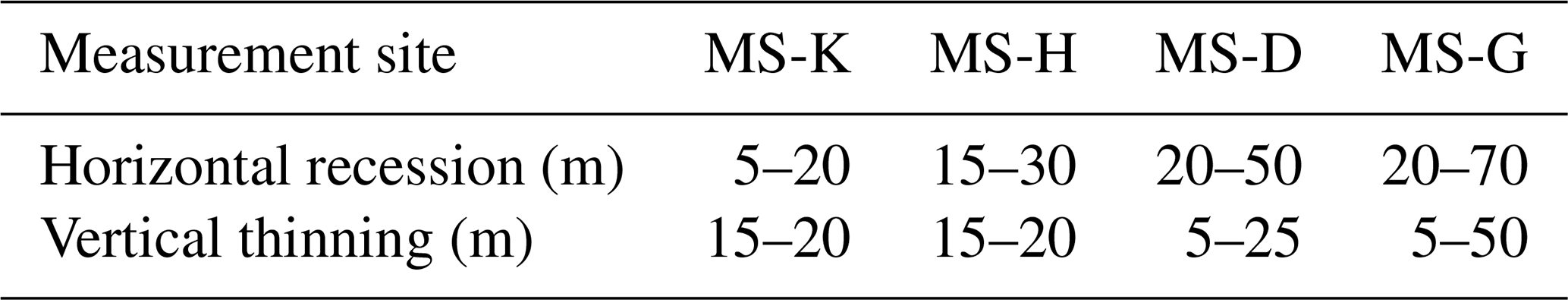
The ascertained horizontal recession and vertical surface lowering rates of the glacier area between 1915 and 2009 for the four measurement sites are shown in Table 1. For MS-K the horizontal recession is about 20 m near the Austriascharte but only 5–10 m at the north face of the Koppenkarstein. The vertical loss there is about 15–20 m. Similar amounts of vertical decline were estimated for the area around the Hunerkogel (MS-H; cf. Fig. 5); the horizontal recession amounts to 15–30 m (Fig. 1). For MS-D the horizontal recession is about 20–50 m; vertically the glacier has lost 5–25 m with the highest losses in the north-west exposition. Around the Gjaidstein site (MS-G), maximum decline rates, both horizontal (up to 70 m) and vertical (15–35 m), were determined.

Table 1 Horizontal recession and vertical surface lowering rates of the glacier areas in the four subregions of interest (Fig. 1) between 1915 and 2009.

3 Methods

We focused on the permafrost distribution in the areas of glacier retreat between 1915 and 2009 (Fig. 3). We followed a multidisciplinary approach primarily including continuous ground surface temperature (GST) monitoring at the surface using a miniature temperature data logger, bottom temperature of the winter snow cover (BTS; Haeberli, 1973) and electrical resistivity tomography (ERT) profiling.

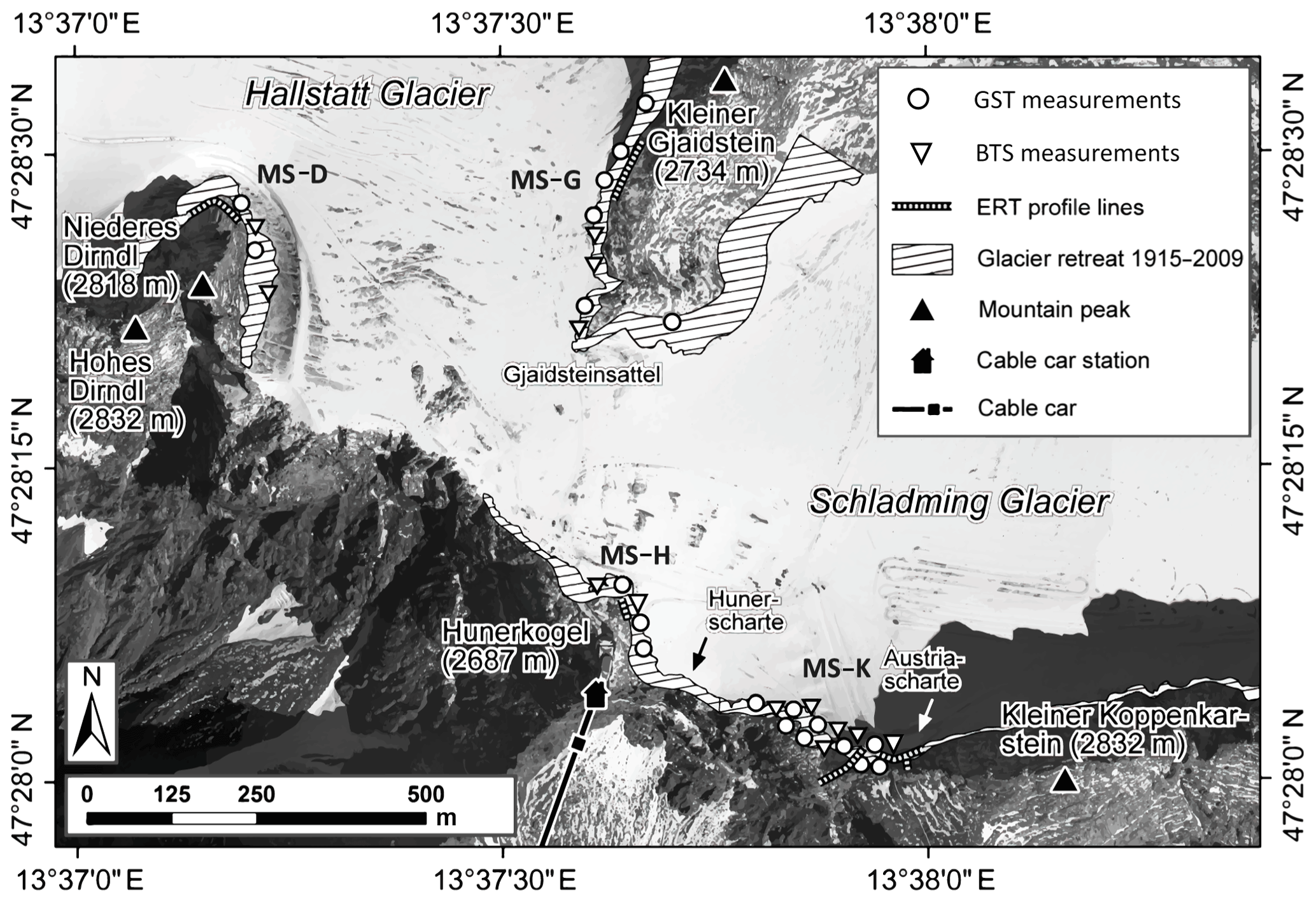
Figure 3 Measurement locations of the different techniques (BTS, GST, ERT) at the studied rock walls. Data source: orthophoto by the province of Upper Austria, 2013.

3.1 Base temperature of the winter snow cover (BTS)

BTS is based on the insulating properties of sufficiently thick snow cover (>1 m), which prevents the ground surface from short-term periodical variations in air temperature (Haeberli, 1973, 1975). BTS is controlled by the heat flow of the subsurface and is distinctly lower above frozen ground. Haeberli (1973) defined temperatures of $<-\mathrm{3}$ ^∘C as permafrost probable, measurements between −2 and −3 ^∘C in the uncertainty range (permafrost possible), and temperatures of $>-\mathrm{2}$ ^∘C as non-permafrost areas. A BTS Pt100 (1/3 DIN class B) thermocouple probe fixed to the bottom of a 3 m long steel rod (Kroneis, Vienna) at the lower end of a 3 m carbon tube was used. Measurements were performed at each point until a constant temperature was registered for at least 2 min. The accuracy of measurements depends on several factors like calibration of the temperature sensor or disturbance of the temperature field by the breakthrough of the snowfield by the probe. A total of 13 BTS points (at each point three measurements within an area of 2 m²; cf. Brenning et al., 2005) were determined at recently glacier-free areas based on the multi-temporal analyses of published maps and orthophotos (Fig. 3) at 2600–2700 m a.s.l. The date of the measurements (20 and 21 March 2013) falls within a period of generally increasing snow cover from 1.5 m (1 December 2012) to 3.5 m (25 March 2013), as recorded by a weather station at the Hunerkogel (snowreporter, 2013). During the 13 BTS measurements, snow depths ranged from 2 to 3.5 m. As pointed out by Brenning et al. (2005), BTS has to be interpreted as a relative measure of ground thermal state and not strictly as a permafrost indicator.

3.2 Ground surface temperature (GST)

To avoid the restrictions of short BTS measurements, additional miniature temperature data loggers (iButtons, e.g. Gubler et al., 2011) were mounted at the near-bedrock surface; iButtons of the type DS1922L (by Maxim Integrated) with a resolution of 0.5 ^∘C and a measurement interval of 1 h were chosen. The sensors were placed in 20 very shallow boreholes in bedrock with a depth of 2 cm (Figs. 3 and 5). Additional protection against moisture was provided by small plastic bags. Preliminary laboratory calibrations of the sensors did not show any notable effects of the plastic bags used. The iButtons (iBs) were placed at the measurement sites at the rock surface beneath the snow pack on 1 January 2013 and removed on 31 July 2013. Therefore, up to 7 months of data were available for analysis.

With the miniature temperature data loggers it is possible to monitor the seasonal temperature fluctuations at the uppermost centimetres of the surface (e.g. Ishikawa, 2003). Such data can be used to assess for instance the thermal conditions under a seasonal snow cover. The winter equilibrium temperature (WEqT) describes temperature fluxes beneath the snow pack and is defined as the mean temperature of stable conditions during February and March. The WEqT depends on the presence or absence of permafrost and on the history of the snow cover at a given measurement site (e.g. Schöner et al., 2012; Kellerer-Pirklbauer, 2019). In the case of the absence of an isolating winter snow cover and, thus, thermal coupling between the atmosphere and the ground, the WEqT approach is not applicable. Interpreted threshold values of the WEqT are identical to the ones of BTS (Haeberli, 1973), defining WEqTs of $<-\mathrm{3}$ ^∘C as permafrost probable and measurements between −2 and −3 ^∘C as permafrost possible (cf. e.g. Schöner et al., 2012; Sattler et al., 2016).

Another important parameter is the zero-curtain period with temperatures of around 0 ^∘C caused by the melting of the snow and isothermal conditions within the snow pack. The basal-ripening date (RD) at the beginning and the melt-out date (MD) at the end frame the zero-curtain period. The RD describes the time when a frozen ground surface is warmed to 0 ^∘C by strong rain-on-snow events or by percolating meltwater (e.g. Westermann et al., 2011). The MD describes on the other hand the time when the snow layer is completely melted, allowing for the ground surface to warm above 0 ^∘C (e.g. Schmid et al., 2012). Late dates for RD and MD as well as a long zero-curtain period are regarded as favourable for permafrost conditions. Particularly, a late MD in summer implies prolonged protection of the snow-covered ground surface from solar heating.

3.3 ERT

For geophysical resistivity measurements, a constant current is applied into the ground through two current electrodes and the resulting voltage differences at two potential electrodes are measured (Knödel et al., 2005). From the current and voltage values, an apparent resistivity value is calculated. ERT is excellently suited for permafrost detection as frozen ground is generally characterised by high electrical resistivity (due to the lack of conducting liquid water) and a strong contrast to the unfrozen surrounding (Hauck and Kneisel, 2008; Schrott and Sass, 2008). To determine the true subsurface resistivity in different zones or layers, an inversion of the measured apparent resistivity must be carried out. We used the RES2DINV software package by Loke (1999) for this inversion procedure. A GeoTom 2D system (Geolog 2000, Starnberg, Germany) with multicore cables was used in the field. Depending upon the local topography, between 24 and 50 electrodes were used per profile. The connection between the electrodes and the rock was established by stainless-steel screws, 12 mm in diameter, which were driven into 12 mm wide and 50 mm deep boreholes. The spacing between two electrodes was 2 m. Thus, the total extent of the survey lines was between 32 and 98 m. Salt water and metallic grease were applied to improve electrical contacts. Figures 3 and 5 show the positions of the ERT measurements at the rock wall of MS-K, MS-H, MS-D and MS-G. The measurements were carried out by means of a Wenner array which provides a particularly sound depth resolution in the central parts of the profile (Knödel et al., 2005; Loke, 1999). We used the robust inversion modelling process in RES2DINV. The model discretisation was set to use an extended model with an enhancement factor of a model depth range of 1.5. Robust inversion delivered very good results in terms of low absolute error (maximum 15.5 %). To assess the quality of the results, the depth of investigation (DOI) method was used (Oldenburg and Li, 1999; Hilbich et al., 2009; Stiegler et al., 2014), which is given by

$$\begin{array}{}\text{(1)}& \mathrm{DOI}(x,y)={\displaystyle \frac{m_{\mathrm{1}}\left(x,z\right)-m_{\mathrm{2}}(x,z)}{(m_{\mathrm{01}}-m_{\mathrm{02}})}}.\end{array}$$

With this technique two inversions of the same data sets are carried out using Eq. (1) but with two different reference models with homogeneous resistivity values m₀₁ and m₀₂ (Hilbich et al., 2009). The first reference value (m₁) is usually calculated from the average of the logarithm of the observed apparent resistivity values. The second reference resistivity value (m₂) is set at 10 times this value. Model regions with DOI index values of >0.2 are considered as unreliable (Hilbich et al., 2009). This empirical method determines the effective depth of investigation (Angelopoulos et al., 2013).

Inversion artefacts are often caused by high resistivities and high resistivity contrasts between frozen and unfrozen subsurfaces and can lead to misinterpretations of the inversion model tomograms. Applying synthetic modelling can be used to confirm the hypotheses drawn from the observed internal permafrost structure of the rock wall. By using the software RES2DMOD (Loke, 1999), simulated data of the expected apparent resistivities were calculated with the same measurement setup as in the field. Gaussian noise of 5 % was added to the apparent resistivities to simulate field conditions (Hauck, 2001; Stiegler et al., 2014). The robust inverted synthetic model was compared to the real inverted data. The modelling process was continued until both inverted data sets converged towards similar tomograms. The final synthetic model was used as a possible representation of the subsurface (Hilbich et al., 2009; Stiegler et al., 2014).

Resistivity category definition

To determine the thermal condition within the rock wall, the resistivity values have to be grouped into different categories. In this study the results of a small-scale geoelectric monitoring station for rock moisture and frost weathering research nearby applied to the ERT profiles at the Koppenkarstein (Fig. 5, MS-K) were used to classify the resistivities. The same GeoTom-2D system with multicore cables for 68 electrodes was used. The connection to the rock was established by stainless-steel screws, 5 mm in diameter, which were driven into 4 mm wide and 1 cm deep boreholes, each 6 cm apart. Thus, the total extent of the survey line was 4.08 m. Additional temperature sensors (Pt1000, GeoPrecision) at a 0, 2, 6, 12 and 18 cm depth gave simultaneous information about the temperature behaviour within the rock. The combined analysis of resistivity and temperature changes at different depths caused by freeze–thaw events provides the necessary information to define the rock resistivity characteristics at different temperatures. The mean resistivities along the whole profile at a 2, 6, 12 and 18 cm depth were compared with the temperature results. Consistent with the laboratory results of Krautblatter et al. (2010), a rapid increase in resistivity from 13 to 30 kΩ m was observed in the temperature range between −0.5 and −1 ^∘C (Fig. 4). The unfrozen rock was characterised by resistivities of up to 13 kΩ m; the transition zone with still unfrozen layers ranged from 13 to 30 kΩ m, and frozen rock had resistivities exceeding 30 kΩ m. Similar thresholds were used by Krautblatter et al. (2007) and Magnin et al. (2017).

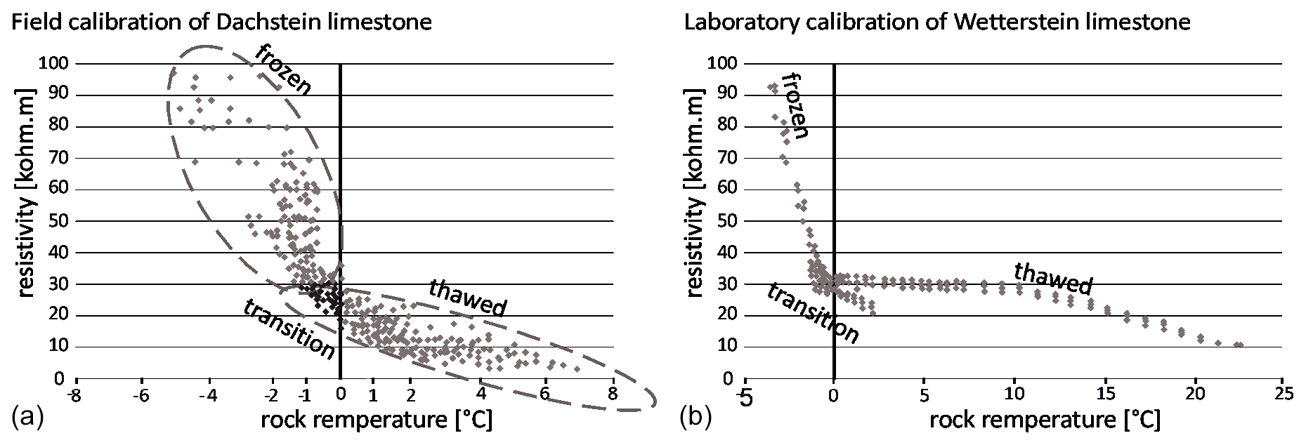
Figure 4 Comparison of small-scale ERT (a) at MS-K and (b) in laboratory (Krautblatter et al., 2010) calibration measurements.

4 Results

4.1 BTS and GST

The ground temperature curves from January to July 2013 display that the winter equilibrium temperature (WEqT) was reached, indicating permafrost, and could be measured at all sites by GST (Fig. 5a–d). At the north-exposed MS-K (Fig. 5a) the mean WEqT of nine GST measurements is −3.9 ^∘C and the mean of the six BTS measurements is −5.0 ^∘C. At MS-H (Fig. 5b) the WEqT (iB-12) and BTS with a north-east aspect is, with −5.2 ^∘C and −5.6 ^∘C respectively, significantly lower than the measured values at the east-exposed rock wall. There, the mean WEqT (iB-13, iB-11) is −3.1 ^∘C and the mean of the BTS values is even higher (−2.2 ^∘C, maximum value of all temperature measurements). The later beginning of RD at this site in July is connected to ski run work with snow redistribution at this site during spring. At MS-D (Fig. 5c) the mean WEqT of the two iButtons with a north-east exposure is −3.6 ^∘C, while the mean BTS, measured as north exposed, is −4.2 ^∘C. For MS-G (Fig. 5d) the results show some more fluctuation in temperature at the beginning of the year (iB-19, February), probably because of less insulation due to a shallow snowpack. The mean WEqT of all GST measurements carried out at the foot of the west- to north-west-exposed slope is −4.3 ^∘C; the mean BTS is −4.5 ^∘C. The WEqT of the south-east-exposed iB-14 is more than 1 K higher (−2.9 ^∘C), which can be explained by much higher direct solar radiation.

Furthermore, the longest durations of the zero-curtain period were measured at sites MS-D and MS-G (Fig. 5c and d), indicating long and more-or-less continuous snow cover depletion at those sites. In addition, the melt-out dates (MDs) at the measurement sites reveal substantial differences in snow cover disappearance between the different sites. The earliest date of MD was calculated for site MS-K (Fig. 5a), whereas the last MD date was calculated for MS-H (Fig. 5b). This implies big differences in thermal conditions, at least when it comes to the moment when the ground temperature measurement sites became exposed to atmospheric warming.

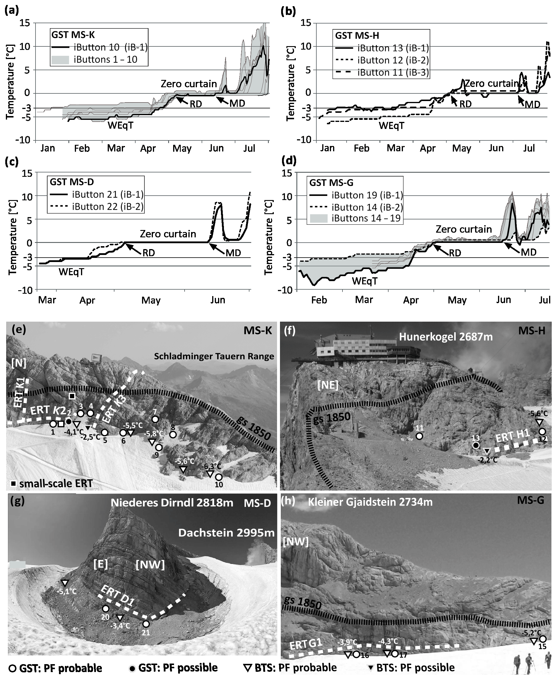
Figure 5 (a–d) GST measurements from January to July 2013. (e–h) Measurement locations of the different techniques at the studied rock walls including interpretation of results of the GST and BTS measurements. The position of the glacier surface (gs) during the maximum of the LIA is indicated at MS-K, MS-H and MS-G (hatched black line). The dashed white lines mark the ERT profiles. GTS locations include numbering; BTS locations include measured temperatures in degrees Celsius. Abbreviations: WEqT, winter equilibrium temperature; RD, basal-ripening date; MD, melt-out date; gs, glacier surface; PF, permafrost. Image data sources: photos by Rode, 4 September 2013.

4.2 ERT

Table 2 gives an overview of the six ERT profiles and their respective ranges of resistivities. The temperature and resistivity classification from Fig. 4 constitutes the base for the interpretation of permafrost existence.

Table 2 ERT profiles information. Abbreviation: PF, permafrost.

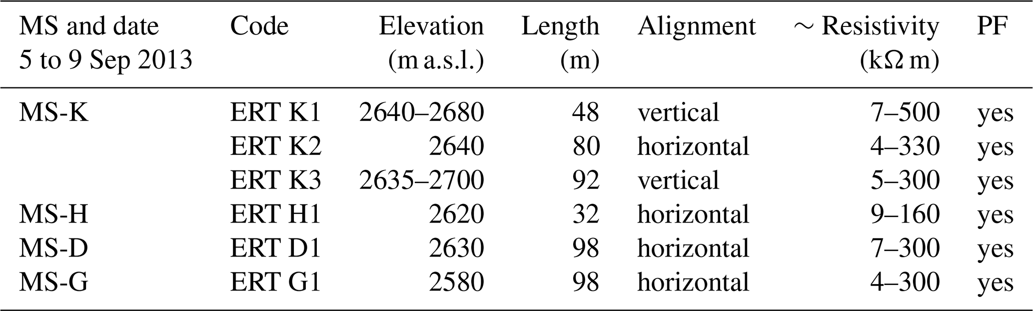
In Fig. 6 all ERT profiles use the same specific resistivity scaling, delineating the three possible thermal conditions. At MS-D, wide areas of high resistivities (>30 kΩ m), interpreted as permafrost, are recognisable beneath a 1.5 m depth. There are also two pronounced zones with resistivities of more than 100 kΩ m. At MS-G, layers with resistivities between 10 and 20 kΩ m are widespread below a 1 m depth. Compared to MS-D the resistivities are lower and more heterogeneous with only two zones of resistivities above 30 kΩ m. At MS-H, only a short ERT profile was possible because of numerous lightning rods installed at the rock wall for the protection of the lift station. Nevertheless, increasing resistivity with rock depth was observed; beneath a 2 m depth the resistivities are between 30 and 80 kΩ m. At the north face of MS-K, three ERT profiles were installed, two of them in vertical settings. These two profiles cross the line where the glacier surface was located during the LIA maximum. The resistivity distribution at ERT profile line K3 with a length of 92 m and a penetration depth of almost 20 m shows higher resistivities (>30 kΩ m) in the upper part and lower resistivities in the lower part (10–30 kΩ m). In the centre of the profile line below a 2 m depth, resistivities of more than 100 kΩ m were observed. At profile line K1, even higher mean resistivities were measured. The section above the 1850 glacier surface shows resistivities on the order of 30–50 kΩ m even at the surface, while below the 1850 line it is in the range of between 5 and 20 kΩ m. Below a 2–5 m rock depth, a massive zone of very high resistivity (>100 kΩ m) is found. The position of the lowest depth of the unfrozen layer and the highest subsurface resistivity corresponds with the LIA glacier surface; downslope of this level, the thickness of the unfrozen surface layer increases. The horizontal profile K2 was measured just above the present glacier surface. Like at the other three horizontal profiles, resistivity steeply increases with depth. In the middle of the profile the surface appears to be frozen (>30 kΩ m) with resistivities increasing to >100 kΩ m at ca. 3–7 m depth. The DOI indexes prove the reliability of all data sets to depths of about 10–15 m (DOI mostly <0.2). The absolute error values of all inversions are between 6.5 % and 15.5 %.

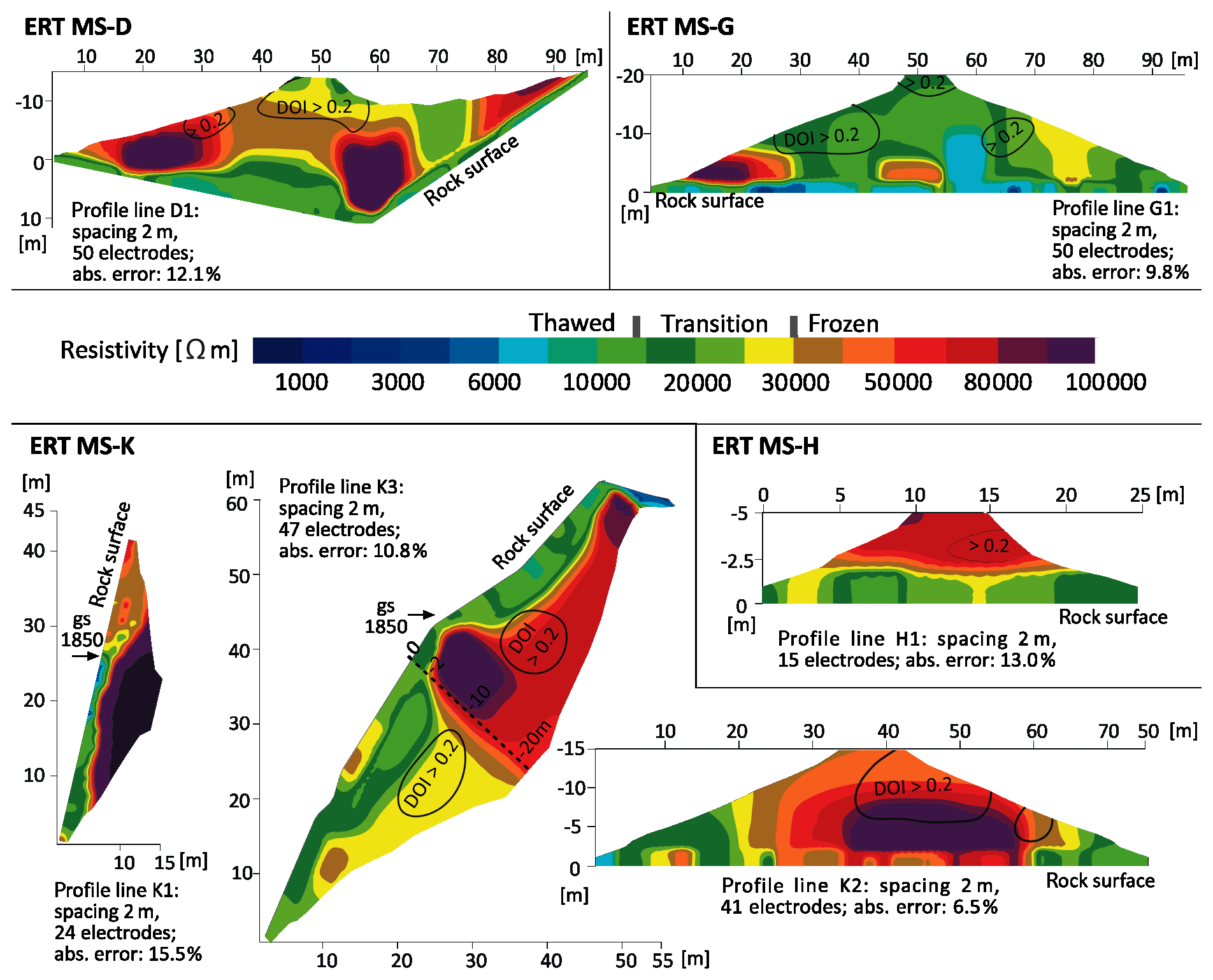
Figure 6 ERT results at MS-D (measurement site Dirndln), MS-G (Gjaidstein), MS-K (Koppenkarstein) and MS-H (Hunerkogel). Abbreviation: gs 1850, glacier surface at ca. 1850.

Box plot diagrams dividing the ERT profiles into 1 m depth sections are shown in Fig. 7. The profile MS-G is the only one with mean and medium resistivities below the 30 kΩ m threshold at all depths. In all other recorded profiles, mean values of >30 kΩ m are reached below a certain depth, which is approximately 3 m at MS-D1, MS-H1 and MS-K1 and 4–5 m at MS-K3. The profile MS-K2 is the only one with mean and median values of ca. 30 kΩ m even in the near-surface layers (surface to a 1.5 m depth). The resistivity increase at MS-K1 between 2 and 3 m is particularly pronounced; at ≥3 m, 100 % of the values are above the 30 kΩ m threshold, pointing to a well-defined permafrost table. At a greater depth (approx. 5–8 m) mean values of 80–100 kΩ m are reached at MS-D, MS-K1 and MS-K2, while the mean is at around 60 kΩ m at MS-K3 and MS-H1.

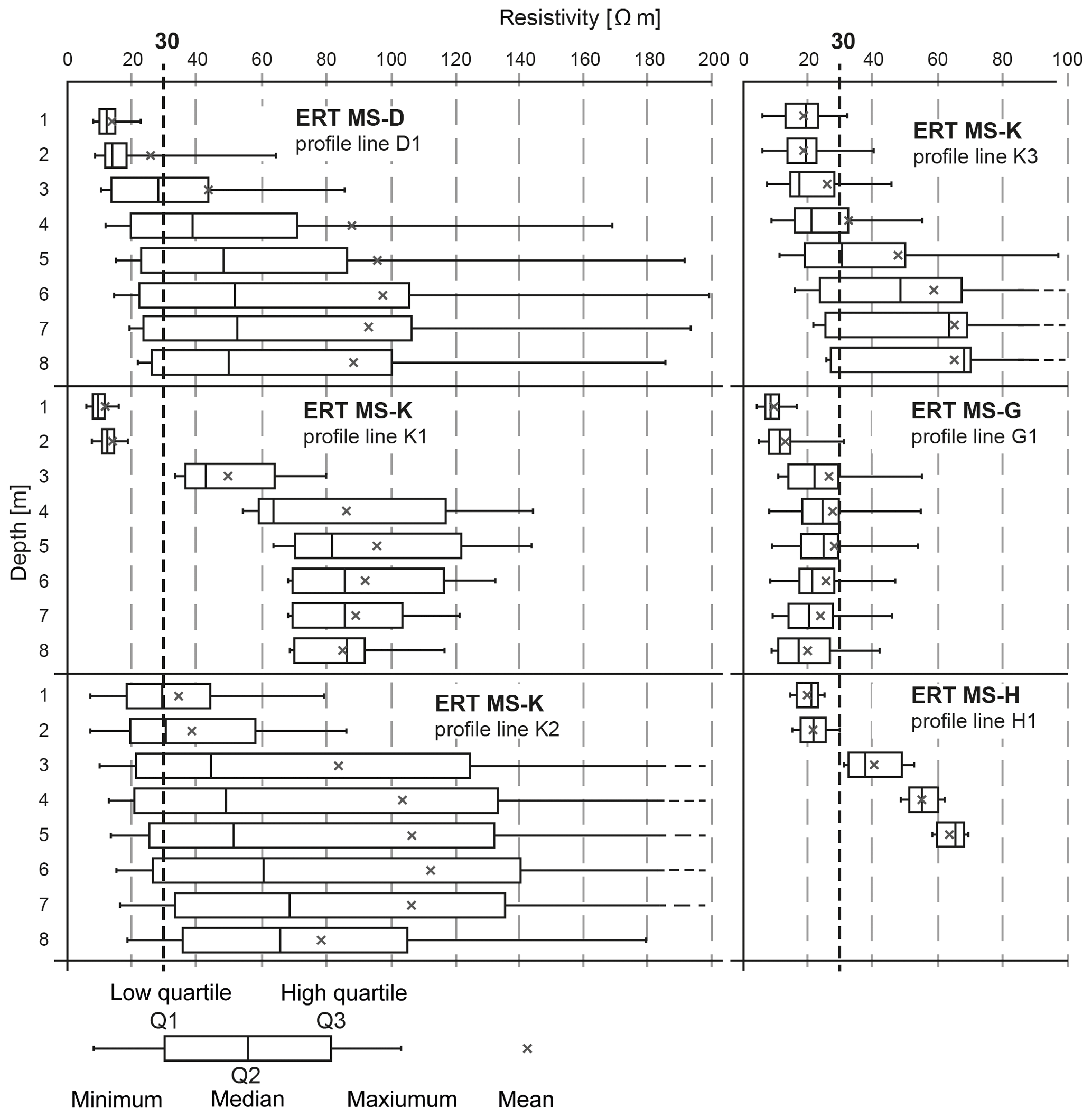
Figure 7 Box plots of measured resistivity at depths from 0 to 8 m over the entire measuring profile. Value range for depth 1: 0< to ≤1 m; 2: 1< to ≤2 m; and so on.

5 Discussion

5.1 Significance of ERT data for permafrost detection

ERT permafrost investigations in bedrock may be error-prone because the resistivity contrast is small between ice, air and certain rock types, as all three nearly behave as an electrical insulator with very high resistivities (Hauck and Kneisel, 2008). Furthermore, the resistivity values for sub-zero ground span a wide range from about 13 kΩ m to more than 30 kΩ m depending on the ice content (Hilbich et al., 2009). At all six ERT profile lines, areas with resistivities higher than 100 and up to 500 kΩ m (Table 2) were measured which, in all probability, represent frozen ground. These exceptionally high electrical resistivities could also be caused by air-filled cavities in the rock; due to karstification of the Dachstein limestone, the existence of caves or small karstified cavities cannot be ruled out. However, the known caves usually occur in pronounced horizontal cave floors, and no cave entries can be found at the elevation of the study sites. Furthermore, the geometrical distribution of high resistivities particularly at MS-K1 and the position of the resistivity anomalies beneath an active layer of plus–minus consistent depth make the cavities interpretation extremely improbable. Furthermore, the interpretation is backed by GST and BTS temperatures.

The use of saline water and conductive grease at the drilled-in screws lowered contact resistances between electrodes and rock and provided satisfactory data quality in terms of root-mean-square errors. The use of the DOI method showed that mainly at high-resistivity changes (between thawed and frozen layers) some areas with a DOI of >0.2 occur and should be discussed with caution (Hilbich, 2009). However, these zones are in positions where they do not affect the general interpretation. On the whole, the DOI analyses showed that all ERT profiles yield reliable results. To exclude resistivity misinterpretations regarding frozen vs. unfrozen conditions, we performed resistivity measurements along a small-scale geoelectric profile combined with temperature measurements at different depths. Krautblatter et al. (2010) performed systematic temperature and resistivity investigations in the laboratory and found a distinct resistivity increase with sub-zero temperatures. They determined 30 kΩ m as the threshold value from which point on the rock (the very similar Wetterstein limestone) is very probably frozen. We were able to confirm these findings in a natural setting. The knowledge of the resistivity range of frozen and unfrozen rock at our sites puts the interpretation on a solid basis. The transition zone with a mixture of liquid water and ice with values of between 13 and 30 kΩ m is characterised by the rapid increase in resistivity at the temperature change from positive to negative (starting around −0.5 ^∘C). During constant freezing and temperatures below −0.5 ^∘C, values higher than 30 kΩ m were measured.

5.2 General distribution of permafrost

Investigations on permafrost distribution in cirque headwalls are scarce due to limited accessibility. Almost all of the measured BTS and GST temperatures point to the existence of permafrost in rock walls recently becoming ice-free of the upper glacier margins which have been subject to glacier retreat since the LIA maximum. This is confirmed by all 2D geoelectric profiles (excluding MS-G) that indicate permafrost at depths of some metres. At all four study sites permafrost layers with resistivities higher than 30 kΩ m occurred. The highest resistivities were found at the MS-K north face, followed by the MS-D site, while at the MS-G and MS-H the resistivities were lower and the borders to the permafrost zones not so pronounced (Fig. 6). The GST results support this resistivity order, with lower WEqTs beneath −5 ^∘C at MS-K and WEqTs between −5 and −3 ^∘C at the three other sites.

Long-term (2004–2015) GST measurements in permafrost at a nearby mountain (Hochreichart, 2416 m a.s.l.) show a general increase in the mean annual ground temperature (Kellerer-Pirklbauer, 2016). The mean annual temperature of 2013 at the Hochreichart site was an average value for the entire 2004–2015 period suggesting that our ground temperature data of 2013 for the Dachstein might be regarded as typical not only for a single year but at least for a decadal timescale.

The Alpine Permafrost Index Map (APIM) by Boeckli et al. (2012a, b) considers the entire European Alps and uses explanatory variables like annual air temperatures, potential incoming solar radiation and precipitation in the permafrost modelling approach. According to the APIM approach, permafrost in our study area is to be found in mostly cold to very favourable conditions. A comparison of our field data with the APIM model leads to the conclusion that our field data support the model (Figs. 5–7). According to the GST and BTS and WEqT classification defining temperatures of $<-\mathrm{3}$ ^∘C as areas with probable permafrost (Haeberli, 1973), all of our sites should be affected by permafrost in favourable conditions. Although the Boeckli et al. (2012a) model assumes permafrost only in very favourable conditions for this site (see http://www.geo.uzh.ch/microsite/cryodata/PF_map_explanation.html, last access: 21 August 2018) for the modelling results), the results at MS-H1 clearly point to permafrost existence.

Evidence of permafrost was found below and above the LIA glacier margin with the lowest active-layer thickness at the very line of the former LIA glacier surface, which means that the imprint of the LIA glacier margin can be found in the resistivity profiles. At MS-K, the thinnest active layer and the highest resistivities of the deeper subsurface were found in the approximate middle of the vertical profiles, corresponding with the 1850 glacier surface. This is particularly well visible at the K1 profile. The flattening of the rock wall at K3 in the elevation of the 1850 surface probably enabled accumulation of infiltrated moisture and the development of massive ice below the surface (−2 to −10 m). Generally higher resistivities (>50 kΩ m) were found in the part of the rock wall above the 1850 margin which has been ice-free for more than 150 years. At the ERT sites near the present glacier surface (MS-K2, MS-D1, MS-G1 and MS-H1) which have been ice-free for a much shorter time, resistivities are lower and the active layer is thicker. The increasing active-layer depth below the LIA margin and the generally very high resistivities around the LIA margin are among the most important observations of the study (see Sect. 5.3).

At MS-D it is difficult to determine the historically highest surface of the glacier, because the glacier surface at the Dirndl mountain is influenced by the mentioned blowout depression at the foot slope of this mountain (cf. Fig. 5g). The investigated part of the rock wall at MS-D1 was probably ice-free even before 1850 (Simony, 1884) and thus exposed to atmospheric conditions for much longer than at MS-K2, MS-G1 and MS-H1. The absence of insulating glacier ice could be the reason for the well-established frozen layers at the left and in the middle of the profile beneath the active layer. However, between those two frozen parts thawing processes occur with resistivities between 10 and 20 kΩ m, mirrored by a wet and fractured rock surface in the field.

5.3 Degradation or aggradation of permafrost?

Significant areas of the study region were affected by glacier recession and glacier surface lowering at the glacier forefield and the surrounding headwalls. The thermal regimes of surface ice and frozen ground can be interconnected and influence each other (Suter et al., 2001; Otto and Keuschnig, 2014). Our results prove the occurrence of permafrost in recently ice-free rock walls. An open question is whether this permafrost has newly formed since glacier recession or whether it was already present under the ice.

At both vertical profiles MS-K1 and MS-K3 (Fig. 6), the largest area and highest resistivities of frozen rock is present near the 1850 glacier ice surface line. Frozen rock at some metres rock depth below the 1850 glacier surface level might be due to (a) permafrost aggradation due to the access of cold air since the beginning of glacier lowering. In this case, the glacier base should have been warm-based. (b) In the case the glaciers in our study area are polythermal (i.e. of type d on Fig. 2.6 in Benn and Evans, 2010), permafrost might exist under the cold-based areas of glacier ice. In this case, the active layer which has developed since deglaciation would indicate current permafrost degradation. As the thermal conditions at the base of the Schladming Glacier are not yet known, this question cannot be definitively clarified, and further research is needed. However, at profile MS-K1 the active-layer thickness decreases from the lowest point of the profile upwards and reaches its minimum at the elevation of the 1850 line. This finding strongly supports interpretation (a) because the higher areas had more time for aggradation than the lower parts. If (b) was right, we would expect the active layer to be thicker where the time span for permafrost thawing was longer with even stronger degradation above the LIA line. An alternative interpretation (c) is that some permafrost existed below the marginal LIA ice cover (e.g. through transverse heat conduction, ice cleft cooling, pronounced randkluft, etc.) without the strict precondition of cold-based marginal ice. However, as the detected permafrost reaches at least 20 m under the former LIA glacier surface, this interpretation is considered unlikely. The timescales involved in building up permafrost are rarely addressed in the literature; however, it is known from glacier forefields that permafrost can form within a few years after glacier retreat (Kneisel, 2003). Furthermore, Magnin et al. (2017, p. 1821) modelled permafrost degradation rates of approximately 5–10 m in 20 years in vertical rock wall settings. Considering these timescales, permafrost aggradation in the up to 150 years after LIA appears to be realistic.

The higher parts of the vertical ERT profiles have presumably been ice-free at least since the onset of the Holocene as judged from general glacier evolution during the entire Holocene in the Eastern Alps (Wirsig et al., 2016). Thus, permafrost in these areas results from significantly different conditions than in the lower parts which have been ice-free for a much shorter period of time; smaller, warmer permafrost layers with lower resistivities should be expected. This assumed pattern is realised at MS-K3 in an ideal way. However, the pattern is opposite at MS-K1 with much higher resistivity in the assumedly younger permafrost zone. The reasons might be drier conditions above the 1850 line and the supply of meltwater below the line leading to more massive ice formations. As further changes in the shallow subsurface might become apparent after some years of observation, repeated measurements might clarify the question of degradation or aggradation of permafrost.

The conditions at the investigated headwalls at Dachstein are typical of many high-mountain cirque settings in which, according to our findings, transient permafrost aggradation is to be expected during glacier surface lowering. Enhanced frost cracking and rockfall around glacier margins have frequently been found or hypothesised (e.g. Matsuoka and Sakai, 1999; Sanders, 2012). As permafrost occurrence increases the sensitivity to frost weathering by increasing cryostatic pressures (Murton et al., 2001; Sass, 2010; Krautblatter et al., 2013), aggradation might provide an additional mechanism for temporarily increased rockfall intensity and cirque erosion.

6 Conclusions and outlook

The methods used have proven their applicability to permafrost mapping and have delivered novel and valuable information on permafrost distribution around the upper margins of retreating glaciers in the Dachstein area. Permafrost was found in all investigated north-facing rock walls between 2600 and 2800 m a.s.l. that were subject to glacier retreat since the LIA maximum. Permafrost preservation (or even aggradation; see below) is thus possible in favourable cold conditions in north faces with MAATs below −2.5 ^∘C (in 2013). Slightly less radiation-exposed sites oriented north-west and north-east show degradation effects with very heterogeneous subsurface ERT tomograms indicating frozen and unfrozen parts. At the only west-facing site, no permafrost could be confirmed. The ERT data are of good quality. The resistivity calibration by using data of a small-scale ERT profile line proved to be a helpful method of delimiting frozen and unfrozen rock, which may aid the interpretation also in other study regions. The ERT interpretation is backed by GST and BTS data.

The most significant finding is the imprint from the LIA ice cover in the vertical ERT profiles K1 and K3 reflected by particularly thin active-layer thicknesses. The existence of permafrost at the former ice-covered positions could be due to the slow degradation of permafrost that already existed under polythermal glacier ice, or to aggradation of permafrost after glacier retreat. Evidence of resistivity distributions in ERT profiles (downslope-increasing active-layer thickness) rather points to aggradation which would be an important finding for research in comparable cirque settings. However, longer-term observations are still necessary to underpin this conclusion.

To clarify the open questions around aggradation vs. degradation, repeated ERT and temperature measurements are necessary, together with temperature measurements at the glacier base to confirm warm-based or polythermal conditions.