the Creative Commons Attribution 4.0 License.
the Creative Commons Attribution 4.0 License.
 | 17 Mar 2020
Quantifying iceberg calving fluxes with underwater noise
Grant B. Deane
Accurate estimates of calving fluxes are essential in understanding small-scale glacier dynamics and quantifying the contribution of marine-terminating glaciers to both eustatic sea-level rise (SLR) and the freshwater budget of polar regions. Here we investigate the application of acoustical oceanography to measure calving flux using the underwater sounds of iceberg–water impact. A combination of time-lapse photography and passive acoustics is used to determine the relationship between the mass and impact noise of 169 icebergs generated by subaerial calving events from Hansbreen, Svalbard. The analysis includes three major factors affecting the observed noise: (1) time dependency of the thermohaline structure, (2) variability in the ocean depth along the waveguide and (3) reflection of impact noise from the glacier terminus. A correlation of 0.76 is found between the (log-transformed) kinetic energy of the falling iceberg and the corresponding measured acoustic energy corrected for these three factors. An error-in-variables linear regression is applied to estimate the coefficients of this relationship. Energy conversion coefficients for non-transformed variables are and 0.92, respectively, for the multiplication factor and exponent of the power law. This simple model can be used to measure solid ice discharge from Hansbreen. Uncertainty in the estimate is a function of the number of calving events observed; 50 % uncertainty is expected for eight blocks dropping to 20 % and 10 %, respectively, for 40 and 135 calving events. It may be possible to lower these errors if the influence of different calving styles on the received noise spectra can be determined.
- Article
(9067 KB) - Full-text XML
-
Supplement
(1881 KB) - BibTeX
- EndNote


1.1 The role of iceberg calving in glacier retreat and sea-level rise
The contribution of glaciers and ice sheets to the eustatic sea-level rise (SLR) between 2003 and 2008 has been estimated to be 1.51±0.16 mm of sea-level equivalent per year (Gardner et al., 2013). Cryogenic freshwater sources were responsible for approximately 61±19 % of the total SLR observed in the same period. Iceberg calving, defined as mechanical loss of ice from the edges of glaciers and ice shelves (Benn et al., 2007), is thought to be one of the most important components of the total ice loss. For example, solid ice discharge accounts for around 32 % to 40 % of the mass loss from the Greenland ice sheet (Enderlin et al., 2014; van den Broeke et al., 2016), and iceberg calving in Patagonia dominates glacial retreat (Schaefer et al., 2015). On the other hand, several studies found that increased submarine melting is a major factor responsible for the observed rapid retreat of tidewater glaciers (e.g., Straneo and Heimbach, 2013; Luckman et al., 2015; Holmes et al., 2019). The exact partitioning between ice mass loss caused by calving fluxes, submarine melting and surface runoff changes geographically and needs to be measured separately at each location. Calving from tidewater glaciers is driven by different mechanisms, including buoyant instability, longitudinal stretching and terminus undercutting (van der Veen, 2002; Benn et al., 2007). Terminus undercutting results from submarine melting and is often considered to be a major trigger of ice breakup at the glacier front (Bartholomaus et al., 2013; O'Leary and Christoffersen, 2013). In support of this idea, the solid ice discharge from tidewater glaciers was found to be highly correlated with ocean temperatures (Pętlicki et al., 2015; Luckman et al., 2015; Holmes et al., 2019), which are expected to increase significantly as a result of climate shifts (IPCC, 2013). Thus, accurate estimates of calving fluxes from marine-terminating glaciers are crucial to both understanding glacier dynamics and predicting their future contribution to SLR and the freshwater budget of the polar seas. Obtaining these estimates requires remote-sensing techniques, which enable the observation of dynamic glacial processes from a safe distance.
Satellite imagery is an effective way to study large-scale, relatively slow changes at the ice–ocean interface, such as the disintegration of the 15 km long ice tongue from Jakobshavn Isbræ in 2003 in Greenland (Joughin et al., 2004). For fast-flowing ice masses, changes of terminus position caused by both calving and glacier flow must be clearly separated. Consequently, satellite imagery is more limited for observing calving events, which typically occur on sub-diurnal timescales and are often not greater than 1000 m3 in volume for most tidewater glaciers in Svalbard or Alaska (e.g., Chapuis and Tetzlaff, 2014). Moreover, a thick layer of clouds, fog or precipitation in the form of snow and rain often makes it difficult to track iceberg calving continuously using optical techniques, such as surface photography or terrestrial laser scanning. These difficulties provide the motivation for investigating the use of underwater noise to quantify calving fluxes.
1.2 Measuring ice discharge – tools and methods
Many different methods have been developed to measure ice discharge from marine-terminating glaciers. Passive glacier seismology, also called “cryoseismology” (Podolskiy and Walter, 2016), is probably one of the most mature, widespread and useful tools; broadband seismometers have been widely installed in remote areas near calving glaciers since the early studies performed by Hatherton and Evison (1962) and Qamar and St. Lawrence (1983). Seismic signals associated with subaerial calving originate from two main mechanisms: (1) the free fall of ice blocks onto the sea surface (Bartholomaus et al., 2012) and (2) interactions between detaching icebergs and their glacier terminus (e.g., Ekström et al., 2003; Murray et al., 2015). The latter interactions, also known as “glacial earthquakes”, are caused by large, cubic-kilometer-scale icebergs of full-glacier height, and the resulting seismic magnitude is not related to the iceberg volume in a simple manner (Sergeant et al., 2016). Higher-frequency (>1 Hz) calving seismicity from iceberg–ocean interactions, constantly detected by distant seismic networks (e.g., O'Neel et al., 2010; Köhler et al., 2015), usually peaks between 1 and 10 Hz (Bartholomaus et al., 2015; Köhler et al., 2015). Both frequency content and amplitudes of high-frequency signatures are found to be independent of iceberg volumes (O'Neel and Pfeffer, 2007; Walter et al., 2012). Bartholomaus et al. (2015) applied generalized linear models to correlate various properties of seismic signals originating at Yahtse Glacier, Alaska, with estimates of iceberg sizes divided into seven classes. In line with previous findings by Qamar (1988), they identified ice quake duration as the most significant predictor of iceberg volume. Based on these studies, Köhler et al. (2016, 2019) successfully reconstructed a record of total frontal ablation at Kronebreen, Svalbard, using seismic data calibrated with satellite images and lidar volume measurements.
Recently, Minowa et al. (2018, 2019) demonstrated the potential of using surface waves generated by falling icebergs to quantify calving flux. They found a strong correlation between calving volumes estimated from time-lapse camera images and the maximum amplitudes of the waves. Other methods for quantifying ice discharge from marine-terminating glaciers, including surface photography (e.g., How et al., 2019), terrestrial laser scanning (e.g., Pętlicki and Kinnard, 2016), ground-based radar imaging (e.g., Chapuis et al., 2010) or terrestrial radar interferometry (e.g., Walter et al., 2019), are usually used for short-term measurements.
1.3 Studying iceberg calving with underwater noise
The approach investigated here is an example of acoustical oceanography, which extracts environmental information from the underwater noise field (Clay and Medwin, 1977). Acoustical oceanography may offer some advantages over other, more well-developed methods for the study of the interactions between land-based ice and the ocean. Low-cost hydrophones are easily deployed in front of marine-terminating glaciers, and acoustic data can be gathered continuously for several months or longer with a high (>10 000 Hz) sampling rate and low maintenance. Measurements are insensitive to lighting conditions such as fog; cloud coverage; and the polar night, humidity and intensity of precipitation. Moreover, acoustic signals recorded in glacial bays and fjords also contain signatures of ice melt associated with impulsive bubble release events (Urick, 1971; Tegowski et al., 2011; Deane et al., 2014; Pettit et al., 2015; Glowacki et al., 2018). While currently no quantitative models exist to estimate melt rates from underwater noise, the potential idea to simultaneously measure submarine melting and calving, two major processes acting at the glacier–ocean interface, is worth mentioning.
Quantifying iceberg calving by “listening to glaciers” was first proposed by Schulz et al. (2008), who suggested long-term deployments of hydrophones (underwater microphones) and pressure gauges, in addition to more traditional measurements of water temperature and salinity, to study signals of ice discharge together with accompanying hydrographic and wave conditions. Following this novel idea, independent studies conducted in Svalbard (Tegowski et al., 2012) and Alaska (Pettit, 2012) showed the first waveforms and spectra of the sounds generated by impacting ice blocks. Pettit (2012) provided an explanation for individual components of the signal, including low-frequency onset, pre-calving activity, mid-frequency block impact, iceberg oscillations, and mini-tsunami and seiche action. Encouraged by these initial results, Glowacki et al. (2015) analyzed 10 subaerial and 2 submarine calving events identified in both acoustic recordings and time-lapse photography made in front of Hansbreen, Svalbard. A spectral analysis of three different calving types, called “typical subaerial”, “sliding subaerial” and “submarine” (see supplementary videos in Glowacki et al., 2015), showed that they radiated underwater noise in distinct spectral and temporal patterns, but all with a spectral peak between 10 and 200 Hz. Most importantly, acoustic emission below 200 Hz was highly correlated with block impact energy in a simple model. The dimensionless coefficient converting impact energy to acoustic energy at the calving impact point was found to be , and the power exponent was assumed to be 1. However, this earlier analysis was limited by the small number of subaerial calving events analyzed (10), lack of a full error analysis and the unrealistic assumption of simple cylindrical spreading of acoustic waves in the water column.
To address these issues, we conducted a new study covering a total number of 169 subaerial calving events observed with time-lapse photography at Hansbreen, Svalbard. Impact energies generated by falling icebergs are estimated with error bars and related to received acoustic signals. The total noise energy resulting from block–water impact is calculated using a standard sound propagation model Bellhop (Porter, 1987, 2011), which requires bathymetry data and sound speed profiles as inputs. Variability in transmission losses associated with sound wave reflections from an idealized, flat glacier terminus is also accounted for. The analysis shows that impact energy is strongly correlated with acoustic emission below 100 Hz. We present a new energy conversion efficiency calculated with this more detailed physical model and demonstrate how cumulative values of kinetic energy and ice mass loss can be found by integrating impact noise over a specified number of subaerial calving events.
2.1 General setting
Hansbreen is a retreating, grounded, polythermal tidewater glacier terminating in Hornsund fjord, Svalbard (Fig. 1). It covers an area of around 54 km2 and is more than 15 km long (Błaszczyk et al., 2013). The glacier has a 1.5 km-wide active calving front with an average height of around 30 m (Błaszczyk et 'al., 2009). The mean thickness and total volume of Hansbreen are estimated to be 171 m and 9.6±0.1 km3, respectively (Grabiec et al., 2012). The surface flow of the glacier is dominated by basal motion in the ablation area (Vieli et al., 2004) and the mean annual flow velocity near the terminus, and its calving flux is estimated to be 150 m yr−1 and 38.1×10⁶ m3 yr−1, respectively (Błaszczyk et al., 2009). The average retreat rate of the glacier during 2005–2010, 44 m yr−1, was more than twice the rate observed between 1900 and 2010 (Grabiec et al., 2012). These characteristics are representative of Svalbard's tidewater glaciers, making the bay of Hansbreen a good study site.
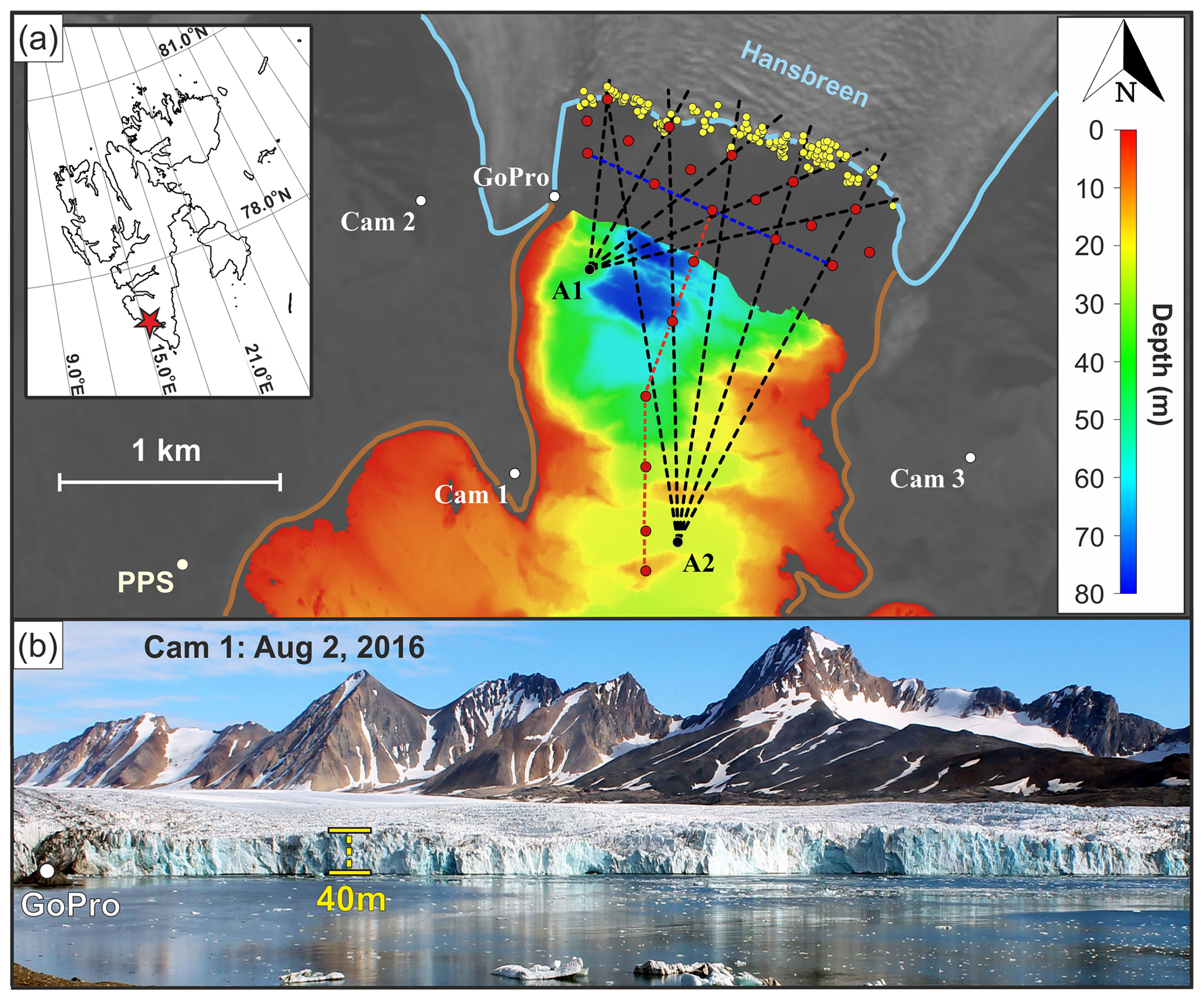
Figure 1A map of the study site (a) and representative cropped time-lapse image taken by Cam 1 (b). (a) Locations of time-lapse cameras, acoustic buoys, calving events and CTD casts are marked with white, black, yellow and red dots, respectively. Colored, dashed lines show transects of CTD surveys oriented perpendicular (red) and parallel (blue) to the glacier terminus. Black dashed lines show the spatial arrangement of bathymetry profiles, which we used to model noise transmission losses. Landsat 8 satellite data collected on 27 August 2016, courtesy of the US Geological Survey, Department of the Interior. Bathymetric data provided by the Norwegian Hydrographic Service under the permit no. 13/G722, issued by the Institute of Geophysics, Polish Academy of Sciences.
Both glacial behavior and the propagation of sound are sensitive to temporal variability in thermohaline structure of water masses in the bay (Pętlicki et al., 2015; Glowacki et al., 2016). The calving activity of Hansbreen is largely controlled by melt-driven undercutting of the ice cliff (Pętlicki et al., 2015). The water temperature and salinity in the center of the bay ranged from −1.8 ∘C to more than 2.0 ∘C and from 30 PSU to almost 35 PSU during 2015 and 2016 (Moskalik et al., 2018). Significant wave height observed in the study site reached a maximum value of around 1.5 m over the period of August–November 2015 (Herman et al., 2019). A geomorphological map of the bay reveals complicated structures in the seabed created by dynamic glacial processes acting after the Little Ice Age, including terminal moraines, flat areas and iceberg-generated pits, to name a few (Ćwiąkała et al., 2018). The water depth along a transect parallel to the glacier terminus ranges from less than 20 to almost 90 m (see Fig. 5 in Moskalik et al., 2018).
2.2 Calving activity and sound propagation conditions
The main dataset consists of more than a thousand subaerial calving events observed between 30 July and 15 September 2016, with three time-lapse cameras and two acoustic buoys deployed in the glacial bay (Fig. 1). At least 20 ice blocks calved each day. It was not always possible to unambiguously identify a calving event in both the image and acoustic datasets; the occurrence of more than one iceberg detachment between the two consecutive images resulted in ambiguity in the acoustic data. Moreover, dense fog, rain or otherwise unfavorable lighting conditions would at times obscure the terminus. From the total calving inventory, a subset of N=169 events were unambiguously matched and analyzed (Figs. 1 and 2). The observer present in the field throughout the data collection phase reported that no anthropogenic sound sources were active during the occurrence of these calving events.
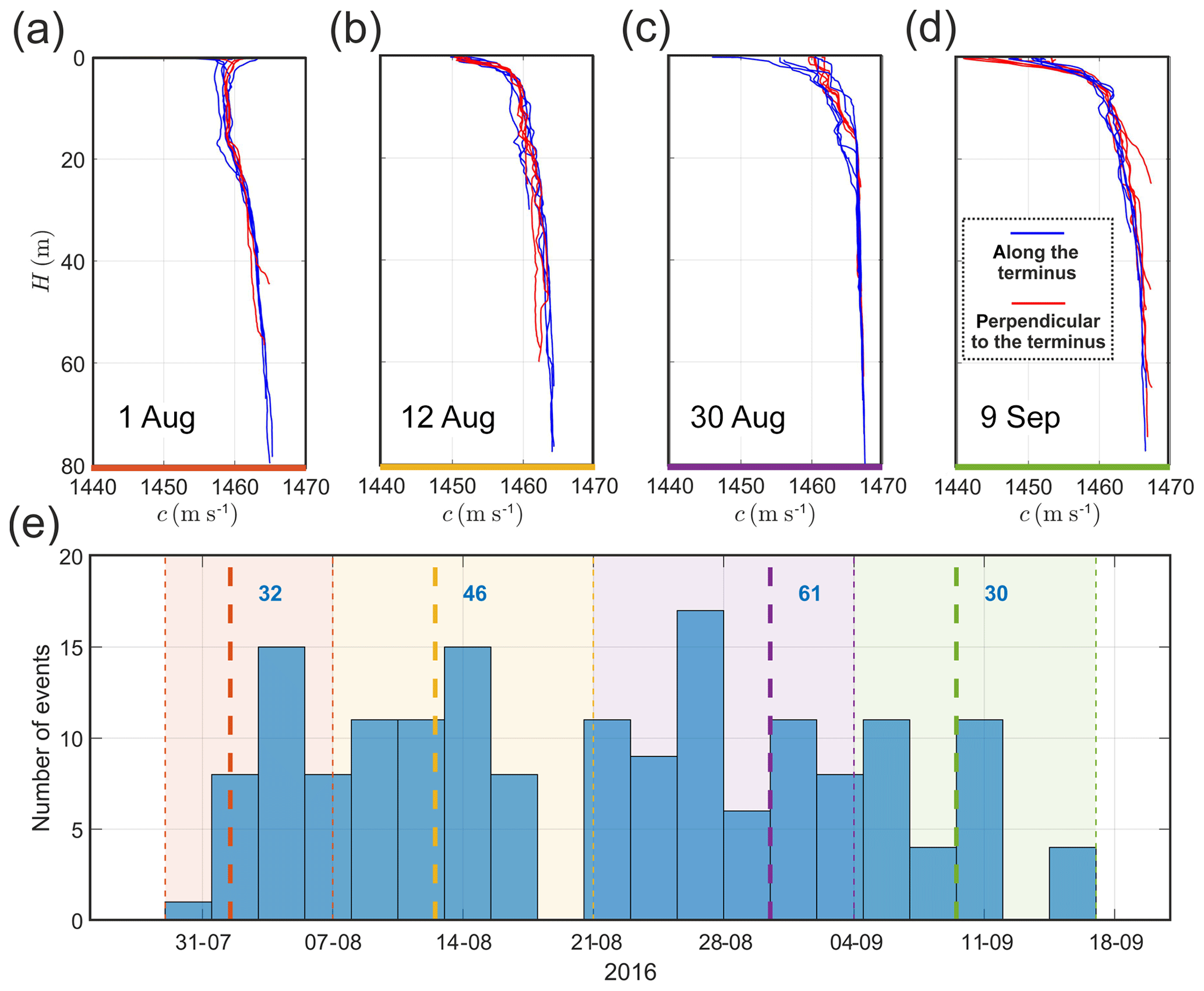
Figure 2(a–d) Sound velocity profiles for CTD surveys oriented perpendicular (red) and parallel (blue) to the glacier terminus, together with (e) the corresponding frequency of calving occurrence. Locations of the CTD transects taken during the study period are shown in Fig. 1 with the same red and blue colors. Thick, dashed lines mark the dates of the CTD measurements. Blue numbers in the lower panel (e) provide the number of calving events assigned to each set of sound speed profiles.
Measurements of ocean temperature and salinity in the bay revealed upward-refracting sound speed profiles, with velocities changing from around 1440 m s−1 just below the surface to almost 1470 m s−1 close to the bottom (Fig. 2a–d). The sound speed gradient between the surface layer and deeper layers, which controls refraction and transmission loss, is driven by fresh meltwater and was clearly increasing during the study period. Moreover, significant differences in sound velocity profiles taken on the same day were also observed between different locations perpendicular and parallel to the glacier terminus, driven by a complex and three-dimensional distribution of the thermohaline field in the bay. The ocean depth between the locations of calving events and the two acoustic buoys varied from 10 m on underwater sills to more than 80 m in the western part of the bay near the terminus (Fig. 3). The bathymetry profiles were very different for the two buoy locations, with a more variable depth observed in the case of the buoy deployed further from the glacier cliff.

Figure 3Bathymetry profiles between the terminus of Hansbreen and the two acoustic buoys: A1 (a) and A2 (b). The spatial arrangement of the transects, which are numbered clockwise, is shown in Fig. 1. The horizontal axis is zeroed at locations of the buoys, marked with black dots. Bathymetric data provided by the Norwegian Hydrographic Service under the permit no. 13/G722, issued by the Institute of Geophysics, Polish Academy of Sciences.
The development of underwater acoustics as a new tool for quantifying calving fluxes requires thorough understanding of the causal relationship between the energy of the ice–water interaction and the resulting noise emission. In this section we discuss all steps that are necessary to complete this task. They are illustrated in Fig. 4 and described in detail in the following subsections. Firstly, a time-lapse camera is used to estimate iceberg dimensions and block impact energies (Sect. 3.1). Secondly, an underwater noise from iceberg–water impact is recorded at a safe distance from the glacier terminus and analyzed to find its amplitude–frequency characteristics (Sect. 3.2). Then, in order to calculate impact noise energy at source, two factors have to be considered: (1) transmission loss in a waveguide, which depends on the distance to the buoy, sea bottom properties along the propagation path and variable thermohaline conditions (Sect. 3.3 and 3.4.1), and (2) the potential contribution of acoustic energy reflected from the underwater part of the glacier terminus on the received calving noise (Sect. 3.4.2). Finally, a simple model relating impact noise energy to the kinetic energy of the falling ice block is proposed (Sect. 3.5). The parameters of this model are derived and investigated further in Sect. 4 to demonstrate a new method for quantifying calving fluxes from underwater noise recordings.
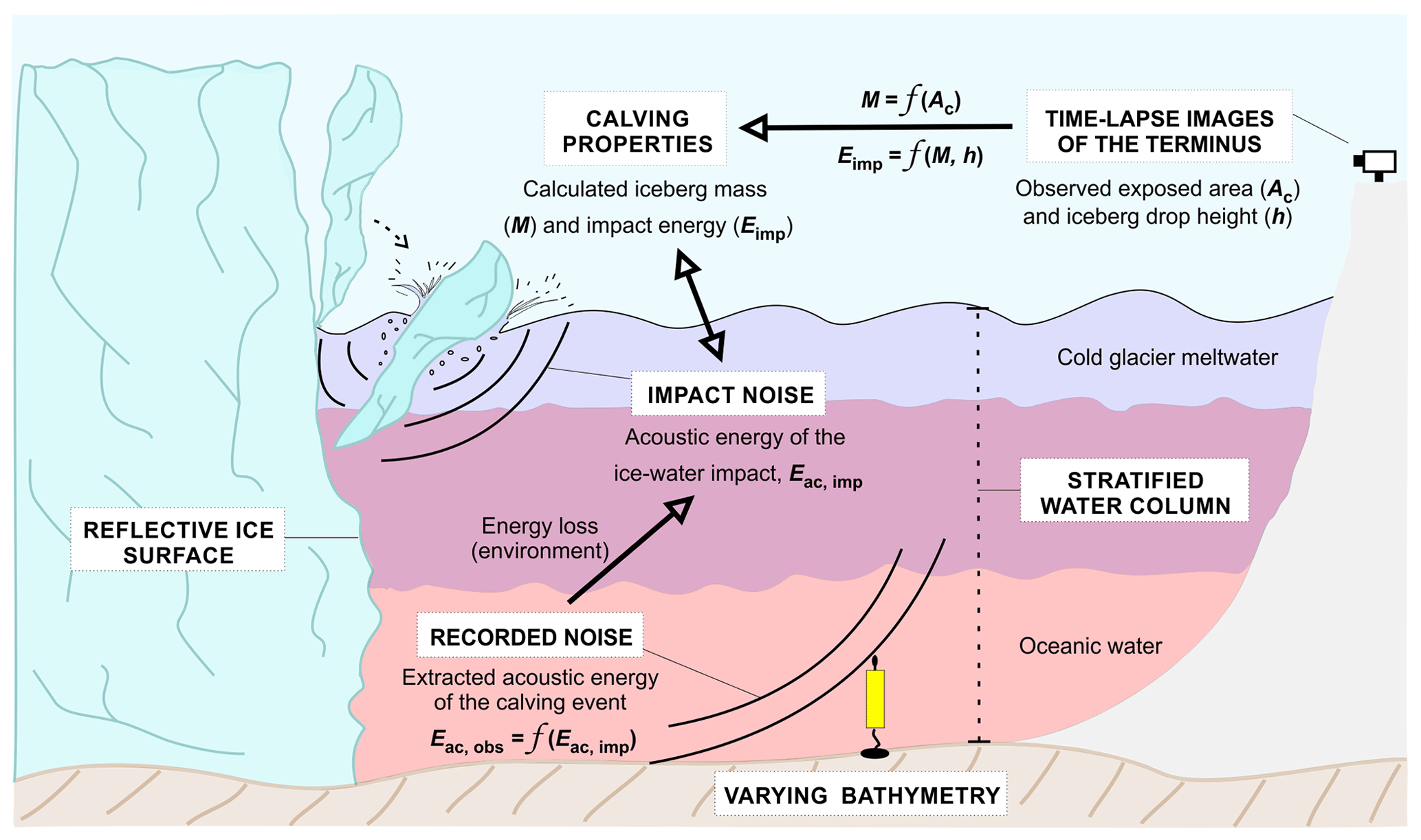
Figure 4A scheme illustrating the application of passive underwater acoustics to measure iceberg calving fluxes. The study consists of (1) time-lapse observation of individual calving events; (2) estimation of ice mass loss and block–water impact energy based on the captured images; (3) recordings of underwater noise at a safe distance from the glacier terminus; and (4) calculation of impact noise energy for given thermohaline conditions, bathymetry along the transmission path and contribution of noise reflected from the ice cliff.
3.1 Photographic observation of calving events
Images of the Hansbreen terminus were taken every 15 min from three locations (“Cam 1–3” in Fig. 1) continuously between 30 July and 15 September 2016 using Canon EOS 1100D cameras (4272 pixel×2848 pixel resolution and 18 mm focal length). The three cameras were not perfectly synchronized, which in fact enabled better separation of individual iceberg calving events occurring shortly after one other. Additionally, a GoPro Hero 3+ camera was placed closer to the terminus to take pictures of the narrow ice cliff segment (“GoPro” in Fig. 1). This camera took images at a much higher rate of 1 s−1 but was not always active during the deployment. Iceberg volume and drop height were estimated using images from Cam 1, which had the most perpendicular orientation to the glacier front of all the cameras. The irregular shape of the ice cliff provided registration features, which were identified in both Landsat 8 satellite images (with resolution of 15 m) and the camera images, enabling a precise localization of calving events.
Following Minowa et al. (2018), the volumes of the calved ice blocks are estimated from the area at the glacier terminus exposed by the calving event. Newly exposed areas are identified from differences between pairs of images taken by Cam 1 (see Sect. S1 in the Supplement for details). The newly exposed area in pixels squared, Aimg, is converted to its real value (in m2), Ac, using the formula
where d is the distance between the camera and drop location and F is the camera focal length. The camera was oriented roughly perpendicular with respect to the calving front (Fig. 1), but precise calculation of the exact angle was impossible due to the limited resolution of the satellite images and large variability in the terminus shape over the study period. Nevertheless, this uncertainty was included in the error analysis (see Sect. 4.3 for details). Guided by previous reports on iceberg dimensions observed in Svalbard (Dowdeswell and Forsberg, 1992), we assumed that the thickness of the calved iceberg is proportional to the square root of the newly exposed area. Then, the iceberg volume is given by
where C is a constant scaling factor, which is reported to be around 0.12 (Åström et al., 2014; Pętlicki and Kinnard, 2016). The drop height, h, is measured as a vertical distance between the sea surface and the midpoint of the falling ice block, converted from pixels to meters. Finally, the kinetic energy of the impacting ice block, Eimp, is given by
where ρi is the ice density, set to be a constant 917 kg m−3, g=9.81 m s−2 is the acceleration due to gravity and M is the iceberg mass. Equation (3) for Eimp is based on the assumption that there is no energy dissipated during the free fall of an iceberg. In reality, energy is dissipated though various physical mechanisms, such as friction between an ice block and glacier terminus, momentum transfer at the early stage of the water entry, drag during the immersion phase, and block disintegration, which can happen at different stages of calving. However, the details of these hydrodynamic processes lie beyond the scope of this work. Because they are not included, Eq. (3) provides an upper bound of the total amount of energy available for noise production during the block–water interaction.
3.2 Impact noise recordings and analysis
The acoustic data were recorded continuously between 30 July and 15 September 2016 using two HTI-96-MIN omnidirectional hydrophones deployed at depths of 40 and 22 m, respectively, in front of Hansbreen (“A1” and “A2” in Fig. 1). The hydrophones have a sensitivity of −164 dB re 1 V µPa−1 and were sampled at a rate of 32 kHz at a resolution of 16 bit. A single mooring system consisted of an anchor, short line and acoustic buoy with a hydrophone, powered by D-cell lithium batteries. Acoustic data were stored on SD cards. The moorings were recovered in their entirety by divers. The horizontal distance between the moorings and locations of calving events ranged from 700 to 1500 m for the closer buoy and from 1800 to 2100 m for the more distant buoy.
The sound produced by calving events was identified manually, based on timing determined from the time-lapse cameras and deviations from median sound level at frequencies below 200 Hz (see Sect. S2 in the Supplement for details). Power spectral density estimates were calculated for each calving event using the Welch method with a 16 384-point fast Fourier transform, a Hamming window of the same size and a 50 % segment overlap to investigate the noise spectra (see Fig. 6). The acoustic energy of the block–water impact at the buoy, Eac,obs, was subsequently calculated by low-pass filtering the noise record at fc and then integrating the mean-square pressure, over the event duration:
The sound speed, c, and water density, ρw, in Eq. (4) were set to 1450 m s−1 and 1025 kg m−3, respectively. The factor of 4π accounts for the surface area of a unit sphere, over which the noise signal must be integrated to obtain total noise energy in joules. The selection of the cutoff frequency of the filter (fc=100 Hz) is discussed in Sect. 4.2. The background noise energy, Eac,bckg, for each event was computed analogously using noise segments of the same length as the corresponding calving signal, recorded just before the ice block impact.
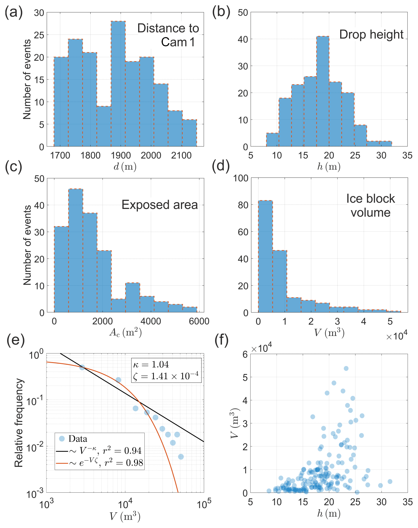
Figure 5Histograms of (a) distances between Cam 1 and locations of calving events, (b) drop heights, (c) exposed areas of the glacier terminus and (d) estimated iceberg volumes. (e) Distribution of iceberg volumes divided into 10 bins, presented on log–log scale. The black line shows best-fit power-law (decay exponent κ) distribution model. (f) Relationship between iceberg drop height and volume. The Pearson correlation coefficient is 0.47 and 0.55 for log-transformed and non-transformed variables, respectively.

Figure 6(a–b) Spectrograms of the acoustic signal generated by the calving event recorded at A1 (a, c, e) and A2 (b, d, f), (c–d) corresponding time-averaged spectra of background (red) and calving (blue) noise, and (e–f) normalized power spectral densities for the entire calving inventory. The calving event for which spectrograms and spectra are shown in panels (a)–(d) started on 30 August 2016 at 08:11:08 UTC. A difference of 10, 20 and 40 dB in Pxx corresponds, respectively, to a factor of 10, 100 and 10 000 in acoustic energy. Noise spectra were normalized using maximum values of the calving signal for each event. Solid lines in (e)–(f) show median normalized spectra.
3.3 Hydrographic and bathymetric data
An overview of the temperature and salinity structure in the study site and its influence on the propagation of sound throughout the bay has been provided by Glowacki et al. (2016). In this study, temperature and salinity profiles were taken on 1, 12 and 30 August and 9 September 2016 with a SAIV SD208 CTD (conductivity, temperature and depth) probe at 11 points, located on transects perpendicular and parallel to the glacier terminus (red and blue dashed lines, respectively, in Fig. 1). Sound velocity was calculated from the CTD data according to the Chen and Millero formulae adopted by UNESCO (Chen and Millero, 1977).
Each calving event has its own, unique set of hydrographic and bathymetric data used for modeling sound propagation, determined in the following way. Firstly, a median sound speed profile was calculated from each set of profiles measured at the same day. Then, a closest median profile was assigned to each calving event according to the time of its occurrence. As a result, four consecutive median sound speed profiles were assigned to 32, 46, 61 and 30 calving events (see Fig. 2). Additional CTD casts were taken in 2017 after significant recession of Hansbreen. These profiles provided information on bottom depths in 11 additional positions located near the glacier terminus position from 2016, which are not covered by the bathymetry data (0.1 m resolution) collected during multibeam surveys (Fig. 1). We selected five bathymetry profiles, separately for two acoustic buoys, that lie along a straight line between the mooring location and CTD stations belonging to the transect that is closest to the ice cliff. Ocean depths in these sections were then interpolated into a 1 m grid using shape-preserving, piecewise cubic interpolation (Fritsch and Carlson, 1980; Fig. 3). Despite the fact that a high level of variability in the thermohaline structure is expected and there is a lack of detailed bathymetry data close to the glacier terminus, the uniquely assigned sound speed profile and interpolated bathymetry are the best available approximation of real conditions prevailing during the study period.
3.4 Attenuation of the calving noise in a glacial bay
3.4.1 Noise transmission loss
The underwater sound of a calving event must travel through the water column before reception at an acoustic buoy, typically several tens of water depths in range or more. Along its path, the signal undergoes multiple reflections from the sea surface and the sea floor and refracts because of changes in sound speed caused by the spatial and temporal variability in the thermohaline structure. These processes result in significant loss of the total signal energy and change the frequency spectrum of the noise observed at the receiver. These effects must be carefully modeled before the calving signature can be quantified in terms of ice block impact energy.
Here we used the standard ray propagation model Bellhop to compute transmission losses, TLprop (Porter, 1987, 2011). The number of beams was set to 2000, with launching angles ranging from −80 to 80∘ with respect to the sea surface. Guided by previous geomorphological studies (Görlich, 1986; Staszek and Moskalik, 2015), we assumed that the dominant sediment type in the study area is a clayey silt; density, sound speed and attenuation were taken to be 1.4 g cm−3, 1530 m s−1 and 0.1 dB m−1 kHz−1, respectively (Hamilton, 1970, 1976). The absorption of sound in seawater is negligible for the low frequencies considered here (e.g., Ainslie and McColm, 1998). Smoothing bathymetry and sound velocity profiles is highly recommended when using Bellhop to predict acoustic energy levels (Porter, 1987, 2011). The bathymetry profile for a selected calving event was spatially smoothed with a moving boxcar filter with a window size of 20λ, where is the wavelength of sound at the frequency of interest. The median sound speed profile calculated from the set of profiles measured at the closest time to the event occurrence was also spatially smoothed with a moving average over 5 m. A baseline (most probable) transmission loss was computed using the environmental data described above, assuming a source frequency of 50 Hz, which corresponds to the peak in the source spectrum (see Fig. 6), and a realistic source depth of 5 mm.
The longest dimension of the calving icebergs is comparable to or greater than a wavelength over the impact noise frequencies, and all points distributed along the ice edge and its close vicinity are considered here to be incoherent noise sources. Accordingly, the incoherent mode of propagation in Bellhop was used to compute TLprop. Finally, to investigate possible variability in TLprop, the simulations were repeated at 100 Hz with the bathymetry-smoothing window changed to 10λ, ocean depth set to the median water depth and the sound speed profile taken to be each of the four median profiles in turn.
3.4.2 Contribution from terminus-reflected noise
The Bellhop model does not easily account for sound reflected from the underwater part of the glacier terminus, which is potentially an important component of the total acoustic energy received at the buoy. The effect of the glacier terminus on observed calving noise, TLrefl, is considered here.
Figure S3 in the Supplement illustrates the direct reflection of sound by the terminus, which is one possible propagation path, but there are more, such as a surface or bottom reflection followed by reflection by the terminus, and so on. All possible paths can be enumerated using a series of image sequences (Deane and Buckingham, 1993) and could, in principle, be investigated. However, we have simplified the problem by considering only energy reflected directly by the terminus, as shown in Fig. S4 (Supplement). The reasoning behind this simplification is twofold. Firstly, the geometry of the problem constrains sound reflected by the bottom followed by the terminus, and sound reflected by the surface between the source and terminus tends to be scattered by the surface waves and bubbles created by the iceberg impact. Secondly, the glacier terminus is rough, resulting in angle-dependent focusing and scattering. Given these complications, which lie beyond the scope of this paper, we have elected to consider only the effect of energy reflected directly from the terminus in comparison with the direct path from source to receiver. As we will show, the greatest effect from this path over the direct path is a 3 dB increase in sound energy and a typical effect is less than 1 dB. These levels are significantly less than the overall effect of the waveguide or inherent scatter in the intensity of sound generated by individual icebergs (see Fig. S5 in Supplement). Moreover, these estimates probably represent an upper bound because the irregular shape of the terminus will tend to scatter incident sound and decrease its contribution when reflected.
The magnitude of sound reflected from the terminus was calculated using a wavenumber integration technique (see Eq. 4.3.2 in Brekhovskikh and Lysanov, 1982). The terminus surface was assumed to be perfectly flat, and the angle-dependent reflection coefficient was estimated using standard formulas for a fluid–solid interface (e.g., see Eq. 1.61 in Jensen et al., 2011). The compressional and shear wave velocities for the ice were taken to be 3840 and 1830 m s−1, respectively, consistent with those reported by Vogt et al. (2008) for bubble-free ice (a review of the literature failed to reveal sound speed values for bubbly ice below 100 Hz). A range of absorption coefficient values were considered in the analysis: from 0.1 to 1.0 dB λ−1 for longitudinal waves and from 0.2 to 2.0 dB λ−1 for shear waves (Rajan et al., 1993; Hobæk and Sagen, 2016). Figure S4a in the Supplement illustrates the relationship between the angle of incidence of incoming calving noise and resulting ice reflection loss. Three regions can be identified in this figure: (1) up to 20∘, the loss is controlled by the ice–water sound speed ratio and typically reaches a value of approximately 7.5 dB, (2) between 20 and 55∘, high attenuation of acoustic energy exceeding 15 dB results mainly from absorption in ice, and finally (3) for larger angles glacier terminus reflects most of the noise energy back to the water. The analysis demonstrates that the ice reflection loss of calving noise depends greatly on the location of a calving event relative to the glacier–ocean boundary and position of the acoustic buoy.
Further analysis was performed using receiver ranges of 700 and 1500 m, which correspond to the terminus-receiver ranges for the experiment. The source frequency was set to the middle of the analysis band (50 Hz), and the source position was varied along the terminus at a fixed distance to the ice cliff of 10 m (Fig. S4b in Supplement). Total energy at the receiver was calculated from the incoherent addition of the direct and terminus-reflected paths and compared with direct path only. The results of this analysis are shown in Fig. S4c (Supplement). At a range of 1500 m, the maximum contribution of ice-reflected path is always smaller than 1 dB because of the steep angles of incidence. At a closer distance of 700 m, the range of possible angles is extended and a maximum increase in received calving noise of around 3 dB can be expected as a “worse-case” scenario. Based on these findings, we assumed a typical contribution from ice reflection of TLrefl=1 dB and corresponding ±1 dB variation around this level.
3.5 Impact energy model
The impact energy model requires an estimate of the total sound energy radiated by a calving event, which can be calculated from
where is total energy loss in decibels (Clay and Medwin, 1977), which includes both propagation loss computed from the Bellhop model and a contribution from energy reflected from the glacier terminus. The subtraction of Eac,bckg from the observed impact noise at the hydrophone, Eac,obs, removes background noise energy from the measurement. The factor containing TLtot transforms the corrected, observed energy into source energy at the impact location. A total loss of −10 dB, for example, corresponds to a decrease of 1 order of magnitude in received energy. Based on visual inspection of the scatterplot between Eimp and Eac,imp, we used a log−log transformation to improve linearity in this relationship. The same type of transformation was revealed by an application of the Box–Cox algorithm, which is often used to normalize regression variables (Box and Cox, 1964). The linear model of conversion between log-transformed energies is given by
Having a=ln η and knowing that , the power-law relationship has a final form given by
Coefficients a and b could be easily derived from an ordinary least-squares linear regression model using log-transformed energies as variables. However, both Eimp and Eac,imp have associated uncertainties, which should be accounted for in the analysis. Therefore, to address this issue, we used the unified equations for slope, intercept and associated standard errors proposed in a model by York et al. (2004). This model belongs to the family of errors-in-variables regression models, which include all uncertainties and always give an answer that is symmetric for both choices of dependent and independent variables. Finally, to exclude outliers from the analysis, we identified all points for which uncertainty in acoustic energy calculated with Eq. (5) is not within 2 standard deviations of the modeled impact noise energy.
This section integrates the acoustic and photographic observations of calving events into a power-law model that quantifies ice mass loss from the noise energy generated by iceberg impact onto the ocean. The model formation begins with a discussion of the statistics of iceberg volume and drop height estimated from the time-lapse images, leading to estimates of the block impact kinetic energy (Sect. 4.1). This is followed by an analysis of the acoustic emission from ice block impacts in terms of its amplitude–frequency characteristics, resulting in an estimate of the total underwater noise energy generated by a calving event (Sect. 4.2). The next section (Sect. 4.3) provides an error analysis of these key variables in terms of uncertainty in measurements of the environment, such as bathymetry and thermohaline structure. The power-law model relating Eimp and Eac,imp is presented and discussed in Sect. 4.4. Finally, based on this relationship, a new methodology is suggested for quantifying the calving flux from the underwater noise of iceberg–water impact (Sect. 4.5).
4.1 The statistics of iceberg volume and drop height
A total of 169 subaerial calving events were captured by time-lapse camera and unambiguously identified with acoustic events (see Sect. 2.2). Individual detachments were unevenly distributed along the active part of the Hansbreen terminus (Fig. 1). The distance to camera, drop height, exposed terminus area and estimated block volume of the calving inventory are summarized in Fig. 5.
The distance between Cam 1 and the locations of block–water impacts varies from 1700 to 2150 m, with an average of 1880 m (Fig. 5a). The drop height spans 8 to 32 m, with a mean value of m (Fig. 5b). The range of the exposed terminus is 125 to 5850 m2 of the ice cliff surface, with an average newly exposed area of 1590 m2 (Fig. 5c). Iceberg volumes were estimated from Ac using Eq. (2) and vary from 0.2×10³ to 53.7×10³ m3. The volume distribution is weighted toward smaller calving events, and approximately 90 % of the ice blocks have a volume of less than 20×103 m3 (Fig. 5d). This observation is consistent with previous reports on the power-law distribution of iceberg sizes in Svalbard (Chapuis and Tetzlaff, 2014), Alaska (Neuhaus et al., 2019), Greenland (Sulak et al., 2017) and Antarctica (Tournadre et al., 2016). A least-mean-squares error analysis of the power-law distribution of iceberg volumes was made using log-transformed variables. The best-fit decay exponent of 1.48 (Fig. 5e) found for the present dataset lies between the exponent of 1.69 for Kronebreen, Svalbard, reported by Chapuis and Tetzlaff (2014), and 0.85 for Perito Moreno Glacier, Patagonia, reported by Minowa et al. (2018). However, we note that some size ranges can be under- or overrepresented due to a limited number of unambiguously matched calving events (169).
Ice block volume versus drop height is shown in Fig. 5f. The highest iceberg volumes are observed for h within the range of 17 and 26 m, which corresponds well to the middle heights of the glacier terminus at the locations of calving events. Inspection of Fig. 5f shows that ice block volume is correlated with drop height; Pearson's correlation coefficient is found to be 0.47 and 0.55, respectively, for log-transformed and non-transformed variables. This is not altogether surprising because the largest blocks of ice cannot fall from the bottom of the terminus, whereas the smaller blocks of ice are not so constrained. The correlation between drop height and iceberg mass is a source of bias in the relationship between ice block volume and impact energy and must be accounted for when inverting acoustic recordings of impact noise for ice mass loss. This issue is discussed in detail in Sect. 4.5.
4.2 The generation of underwater sound by iceberg calving
Figure 6 shows a comparison between power spectral density estimates for underwater noise from calving and background noise recorded by buoys A1 and A2. Spectrograms of the noise generated by a randomly selected calving event are shown in Fig. 6a and b. The computed difference in time of arrival between the two receivers was subtracted from the more distant receiver for better juxtaposition. The two primary sources of sound in the spectrograms are ice melt noise and the underwater noise of calving.
The signal of ice melt, driven by impulsive bubble release (Urick, 1971), is most pronounced between 1 and 3 kHz and corresponds well to the spectral bands reported in previous studies (Deane et al., 2014; Pettit et al., 2015). This signal remains stable during the short observation period. The underwater noise of calving is a by-product of the interaction of the falling iceberg with the ocean. The noise is evident from 2 to 8 s in the recording at frequencies below 1 kHz. The acoustic intensity varies in both time and frequency. This variability is almost certainly driven by different noise production mechanisms active at different phases of the calving event (see the high variability in power level between 2 and 4 s, for example). As pointed out by Bartholomaus et al. (2012), low-frequency seismic signals from the impact of ice blocks on the sea surface are generated by three major mechanisms: (1) the transfer of momentum from the falling block to seawater, (2) iceberg deceleration due to buoyancy, and (3) the collapse of an underwater air cavity and subsequent emergence of Worthington jets (e.g., Gekle and Gordillo, 2010). The last mechanism is only possible during total submergence of the ice block, the occurrence of which depends mainly on iceberg dimensions and drop height. Therefore, some calving events may not result in the creation of an air cavity. Moreover, falling icebergs are often fragmented or impact the water at various angles, which certainly modifies all three mechanisms of noise production. The influence of calving style on sound emission lies beyond the scope of this work but is likely a significant factor in the variability in sound generation by blocks of similar mass and drop height, as discussed in Sect. 4.4.
The unique patterns in the time and frequency distribution of calving noise potentially contain information about the details of the calving event. However, attention here is restricted to a single number, which is the time and frequency integrated energy in the sound field generated by the iceberg impact. Calculation of this number requires selection of the start and stop times of the impact noise and the frequency band over which the noise exceeds background sound levels. The significant increase in noise power accompanying calving allows easy identification of event start and stop times, and these have been selected manually for each event analyzed (see Sect. S2 in the Supplement). Figure 6c and d show a 6 s average of noise power spectral density for a calving signal (blue) and background noise recorded just before the event (red). There is a difference between the calving and background noise levels at frequencies up to 700 and 400 Hz for buoys A1 and A2, respectively. The maximum increase in received noise power from calving is approximately 40 dB for both buoys, which corresponds to a factor of 10 000 in acoustic power. The results in Fig. 6 show that the appropriate band of frequencies to consider for calving impact noise ends at around 1 kHz. However, an upper frequency limit of 100 Hz was applied in further analysis to yield the highest correlation between the impact energy and the received acoustic energy.
The variability in calving noise power across the entire dataset is shown in Fig. 6e and f. The normalized power spectral densities of calving events and background noise are plotted as blue and red dots, respectively. A normalization factor is chosen for each calving event and taken to be the highest power level in decibels during the event. The same normalization factor is used for both calving and background noise. Calving signatures are clearly distinguishable from the background noise across the entire dataset. However, the calving noise power is noticeably more variable at receiver A2 than A1. There are two possible reasons for this discrepancy. Firstly, spatial dependency of the thermohaline structure is expected to be significant along the longer propagation path to A2. Secondly, the signal-to-noise ratio for receiver A2 is lower and more variable than at A1, as a result of the shallower depth of the hydrophone (22 m at A2 versus 40 m at A1) and greater exposure to noise coming from outside the bay (see Sect. S4c in the Supplement for more details). The increased scatter in calving noise observed at location A2 resulted in a decrease in correlation between total impact energy and impact noise (see Table S1 in the Supplement), and data from this buoy are not considered further.
4.3 Details of error analysis
There are two sources of uncertainty for block–water impact energy and impact noise energy: measurement error and uncertainty in the state of the changeable environment, which is impossible to characterize completely. Estimates of these uncertainties can be made for the various stages of the analysis connecting impact noise to ice mass loss, and these are discussed below.
4.3.1 Uncertainty in block–water impact energy
Assumptions and approximations need to be made when determining the kinetic energy of the falling ice block from time-lapse images. Uncertainties in estimates of the block–water impact energy result mainly from the conversion of the exposed area at the glacier terminus into ice block volume (see Sect. 3.1). Moreover, additional errors are associated with the details of image analysis, related to the spatial resolution of the time-lapse photography (∼80–100 pixels per terminus height) and imprecise determination of the locations of calving events. The total uncertainty in kinetic energy is difficult to estimate accurately due to several factors, including but not limited to (1) the irregular shapes of the icebergs, (2) poorly understood site-to-site variability in the scaling factor C, and (3) space- and time-varying orientation of the glacier terminus with respect to the camera. However, following Minowa et al. (2018), we assume that the errors in Aimg, d, C and h are not larger than 10 %, 5 %, 20 % and 5 %, respectively. The uncertainty in Ac, computed with Eq. (1), is 14 %. Then, since uncertainties in the estimates of ice volumes and drop heights are dependent, the total error bound in the kinetic energy of the impacting ice block is estimated to be approximately 33 %.
4.3.2 Errors in calving-generated acoustic energy
Uncertainties in estimates of the iceberg impact noise result from three major sources: (1) spatial and temporal variability in the thermohaline structure in the glacial bay (see Fig. 2a–d), (2) complicated bathymetry along the propagation path, which depends on the location of calving event (see Fig. 3), and (3) angular and frequency dependence of sound reflection from the underwater part of the glacier terminus (see Fig. S4 in Supplement). Considering both transmission and reflection losses, the total loss of acoustic energy generated by block–water interaction, TLtot, ranges from −47 to −57 dB (see Fig. S5 in the Supplement), corresponding to a factor of 10−5 and 10−6 in acoustic energy at the source across the entire inventory of calving events. We combined variability in transmission and ice reflection losses for the entire calving inventory to estimate a representative uncertainty of 33 % in acoustic energy for each individual calving event at its source.
4.4 Relationship between the block–water impact and acoustic energy
Estimating calving ice mass flux from calving noise is based on the idea that these two quantities are correlated. Figure 7 shows a scatterplot of impact noise, Eac,imp, against impact kinetic energy, Eimp, for the entire dataset. The dashed black line shows the result of a regression analysis of the power-law relationship shown in the figure legend. The acoustic energy generated by a calving event was calculated from the acoustic pressure time series using Eqs. (4) and (5) with manual selection of integration time (see Sect. S2 in the Supplement) and after low-pass filtering at a cutoff frequency of 100 Hz (see Sect. 4.2). The kinetic energies of the falling ice blocks were derived from Eq. (3) using their masses and drop heights estimated from the camera data (see Sect. 4.1).
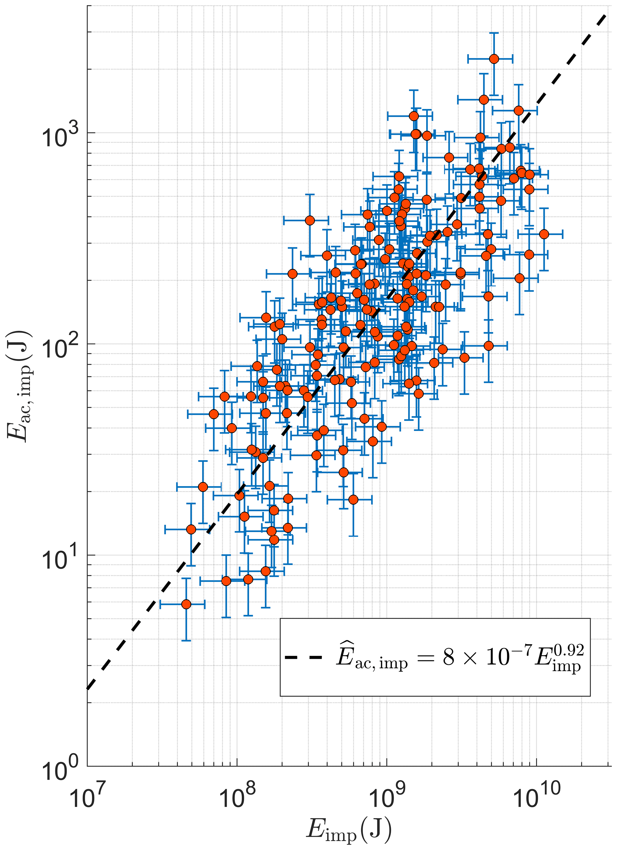
Figure 7Relationship between the block–water impact energy and underwater acoustic emission below 100 Hz. Uncertainties are marked with blue whiskers and were estimated to be 33 % for both variables. The remaining scatter in impact energy is most likely caused by different calving styles and an associated variability in source mechanisms. The results with inclusion of outliers are shown in Fig. S6 in the Supplement (see text for details).
The range of energy estimates is large, roughly 2.5 orders of magnitude for both, and there is clearly a strong correlation between the energies across their entire range. The regression coefficient r=0.76 was found between the log-transformed variables for p<0.0001. If uncorrected calving noise energy and signal duration are used instead of Eac,imp, the correlation drops to 0.71 and 0.61, respectively (Table S1 in the Supplement). After removing two outliers and applying an error-in-variables linear regression (see Sect. 3.5 for details), the best functional relationship between acoustic energy and impact energy was found to be a power-law relationship given by Eq. (7), where % and %, respectively, for the multiplication factor and exponent of the power law. For completeness, this analysis was repeated, including the two identified outliers, and the results are shown in Fig. S6 (Supplement). Glowacki et al. (2015) previously reported and b=1, which gives an impact energy that is 2.5 orders of magnitude higher in comparison to the results presented here (see Fig. S7 in Supplement). This discrepancy is due to the overly simplified propagation geometry assumed in the earlier study – simple cylindrical spreading loss and no sound reflection from ice terminus – which resulted in an underestimate of the impact noise energy.
The multiplication factor η can be thought of as a conversion efficiency of kinetic energy of a falling iceberg to impact noise energy. The small value of η shows that only a tiny fraction of the ice block energy is transformed into underwater sound, which then propagates from the point of impact to the acoustic receiver. A low conversion efficiency is consistent with observations reported for other physical mechanisms of underwater noise generation. For example, only of the energy dissipated by a breaking surface wave on the ocean is radiated as sound (Loewen and Melville, 1991). Similarly, the conversion efficiency of the impact energy of a 1–5 mm scale raindrop falling on the sea surface to underwater impact noise is in the range 10−9 to 10−8 (see Eq. 4.6 in Guo and Ffowcs Williams, 1991, and Gunn and Kinzer, 1949).
Despite a strong correlation between impact energy and impact noise, there is also a significant scatter in impact noise energy (roughly a factor of 10) for a given value of kinetic energy. This spread in values can be only partly explained by errors in the energy estimates, which are indicated by blue whiskers in the Fig. 7. The scatter is presumably caused by differences in noise generation between individual calving events. The consequence is that estimating the impact energy of an individual calving event from the total noise energy it radiates is accompanied with significant uncertainty. However, because of the overall strong correlation between noise and impact kinetic energy, it is possible to predict the total impact energy summed over a finite number of calving events, provided the inventory is large enough. The uncertainty in individual events tends to average out if enough events are considered, as discussed in Sect. 4.5.
4.5 Estimation of ice mass loss from the calving noise
Figure 7 and Eq. (7) show that the relationship between iceberg impact energy and calving noise can be modeled robustly with a power-law relationship, providing a means of estimating impact energy from calving noise. Although there is significant variability in doing this on an event-by-event basis, low-error estimates of cumulative impact energy can be made using Eq. (7) if enough events are added together. Once found, the cumulative impact energy can be converted into an estimate of iceberg calving flux as follows.
The cumulative modeled ice mass loss from N observed calving events is related to the cumulative impact energy, as inferred from the acoustic signal, by
where g is the acceleration due to gravity, hj is the height of the center of mass of the jth iceberg before separation from the glacier terminus, is the mass of jth iceberg determined from its underwater impact noise and is the kinetic energy of impact of the jth iceberg. The cumulative ice mass lost through calving would be trivial to compute from Eq. (8) if the mean iceberg drop height were independent of the iceberg mass, but this is not the case (see Fig. 5f). Icebergs that extend a significant fraction of the exposed terminus height have a minimum drop height that is larger than the minimum drop height possible for smaller icebergs. For this (and possibly other) reasons there is a correlation between iceberg drop height and iceberg mass, the consequence of which is that hj cannot be moved outside the sum on the left-hand side of Eq. (8). The correlation is dealt with by introducing the mass-weighted drop height:
It follows immediately from Eqs. (8) and (9) that the cumulative mass sum is given by
which provides a means of computing the calving flux, since the kinetic energy of iceberg impact can be estimated from its underwater noise using Eq. (7).
We are left with the problem of computing . To address this issue, a new variable is defined by
where is an observed, average drop height. Let us now assume that, for sufficiently large N, can be approximated by
The right-hand side of Eq. (12) is in terms of iceberg mass inferred from the camera observations, providing a means of computing the mass-weighted drop height, , on a glacier-by-glacier basis. The constant and resulting mass-weighted average drop height are estimated to be 1.13 and 20.7 m for Hansbreen.
Equation (10) for the cumulative calving mass flux contains significant uncertainty when N is small because of the large scatter in the total underwater sound energy generated by calving events with similar impact energies (see Fig. 7), but the uncertainty reduces as N increases. How large must N be to achieve a desired degree of uncertainty? To answer this question, a Monte Carlo simulation of cumulative ice mass loss was performed using n calving events randomly selected (with replacement) from the entire inventory of calving observations (for which N=169). This selection is repeated ψmax times for each }, noting that the total number of possible sets of calving events (and associated cumulative kinetic energies and masses) is given by
From Eq. (10), the cumulative mass sum for a given number of randomly selected calving events n and iteration ψ is
where is calculated from Eqs. (11) and (12) using the N=169 observed calving events. The modeled mass in Eq. (14) corresponds to in Eq. (10), where . The inferred, cumulative ice mass normalized by the cumulative ice mass measured with the camera is then given by
where β, for a specified n and averaged over ψmax iterations, can be expressed as
We set nmax to 1000 and ψmax to 10 000 to determine the statistical properties of β over a broad range of sample sizes. We note that the probability of randomly obtaining the same set of calving events is vanishingly small for the chosen ψmax (C≫10 000 for n≥3; see Eq. 13).
Figure 8 shows the mean, , and standard deviation, βn,std, of the statistical distributions of computed from the Monte Carlo simulation. The correct and unbiased estimate of the mean ice mass flux ratio is , which is indeed the asymptotic value reached for large n. As expected, the temporal resolution of the acoustic technique increases with increasing calving activity. The estimated cumulative mass is within 20 % and 10 % of the expected value when integrating over 40 and 135 ice blocks, respectively (Fig. 8). The number of calving events required for a specified level of uncertainty translates into an observational timescale that must be met depending on calving rate. For example, at Hansbreen an uncertainty in ice mass flux of about 20 % is expected when integrating over 2 d of acoustic measurements, corresponding to a calving rate of 20 icebergs per day. The time interval required for a specified level of uncertainty will vary between glaciers and over time. For example, some glaciers calve more than 10 ice blocks hourly (e.g., How et al., 2019), leading to a relatively short time interval requirement.
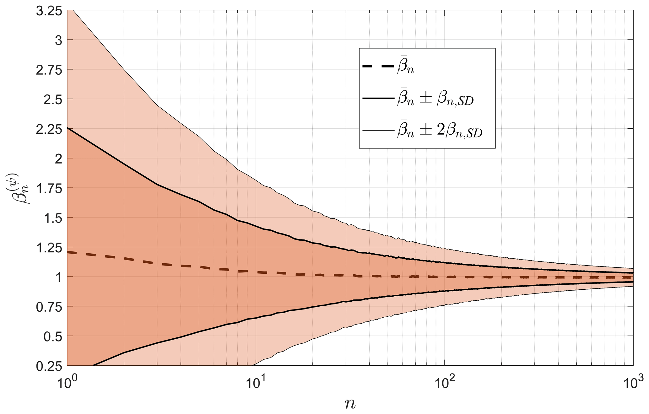
Figure 8The ratio between modeled and observed cumulative ice mass loss computed using the Monte Carlo method, with n events randomly selected (with repetition) from the entire calving inventory. The selection procedure was repeated 000 times for each n. See text for details of the modeled ice mass loss calculation. The thick and thin solid lines, respectively, denote 1- and 2-standard-deviation boundaries of the distributions.
This study demonstrates a new methodology for measuring iceberg calving fluxes from the underwater noise recordings taken in a glacial bay. However, a number of factors have to be considered before the method is adopted for long-term monitoring of ice mass loss, including data retrieval and storage, power supply, instrument clock drift, automatic detection of calving events, and potential site-to-site variability in the model parameters. These aspects are briefly discussed below.
5.1 Data collection and automatic detection of calving events
We collected the underwater noise data continuously with two light moorings powered by D-cell lithium batteries. Moorings were later recovered by divers with inflatable lift bags. The relatively shallow water at locations A1 and A2 (<45 m) made diving possible. Acoustic monitoring of calving fluxes in deeper study sites will require the use of acoustic releasers in order to retrieve the recording equipment remotely from a boat or ship. In fact, an example of calving signals recorded at location A2 shows that very shallow water prevents effective transmission of the calving noise and decreases the signal-to-noise ratio at low frequencies (see Fig. 6 and Sect. S4c in the Supplement). Further issues for consideration are data storage and clock drift. Acoustic data can be stored on SD cards, which are power-efficient and capacious. The internal clock drift during the recording period is expected to be not greater than 30 s per month, given that quartz oscillators that hold stability of at least ±10 ppm are typically used in data acquisition systems. Low-cost acoustic recorders can be added to the existing monitoring programs, where heavy moorings are used to study processes taking place at the ice–ocean interface, including water circulation, heat exchange or sediment transport, for example (e.g., Straneo et al., 2019). Moreover, data collection can be made real time with a cabled or wireless link to shore, but we have not tested this possibility yet. The problem remains with automatic extraction of the calving signal from long-term, continuous acoustic recordings. Calving events are clearly distinguishable from the noise of ice melting in spectrograms of the acoustic record at frequencies below 1 kHz (see Fig. 6a), which is promising in terms of automatic event detection. However, it should be borne in mind that there are other, low-frequency sound sources active in a glacial bay. For example, calving or the disintegration of bigger icebergs could be mistaken with glacier calving events (see Richardson et al., 2010). Moreover, distinguishing between subaerial and submarine calving can be difficult, as found during passive seismic surveys (see Köhler et al., 2019). These issues await further investigation.
5.2 Variability in the model parameters
In addition to a minimum sample size for a specified error requirement (see Sect. 4.5), there are five other parameters that must be known to compute reliable estimates of ice mass flux from calving noise: the mass-weighted, average iceberg drop height, , the conversion coefficient from the newly exposed area to block volume, C, the conversion efficiency from impact to acoustic energy, η, the power-law coefficient, b, and the transmission loss from the glacier terminus to the hydrophone position, TLprop. Errors in these parameters are important because they affect the uncertainty and temporal resolution of the acoustic measurements of calving fluxes (see Figs. 7 and 8).
The problem of how site-specific these parameters are lies beyond the scope of this work, and similar studies should be performed for different tidewater glaciers to obtain quantitative answers. Nevertheless, we briefly discuss here some techniques for measuring or modeling these parameters along with environmental factors driving variability between sites. Noise energy loss is usually calculated using a standard propagation model, such as the Bellhop model used here. Propagation models require sound speed and bathymetry profiles as inputs, making hydrographic and CTD surveys an essential component of the acoustic measurements of calving fluxes. Although the thermohaline structure of a glacial bay is complex and three-dimensional (e.g., Jackson et al., 2014), patterns of temperature and salinity that are sufficiently characteristic of prevailing conditions in the bay can be identified from limited field measurements and used for propagation model inputs (Glowacki et al., 2016). Moreover, it might be possible to use signal duration instead of the corrected noise energy to estimate calving fluxes (see Sect. S5 in the Supplement) as an alternative when no information is given on bathymetry and/or sound speed profiles. We anticipate that there is a high uncertainty associated with the conversion coefficient from the newly exposed area to block volume, which likely varies between glaciers characterized by different surface velocity, thermal regime, hydrology, terminus height, etc. This parameter can be determined more accurately for a specific glacier using short-term lidar measurements or image analysis, e.g., structure from motion or stereo photography. These techniques can also provide an estimate of the mass-weighted, average drop height. The value of is expected to be close to one-half of the average terminus height (in its active part) because the size of ice blocks breaking off from the top or bottom part of the ice cliff is limited (see Fig. 5f). We hypothesize that the remaining two parameters, the energy conversion efficiency and power-law coefficient, are likely stable between glaciers of similar geometry and flow dynamics.
The study presents a new methodology for quantifying the calving flux from the underwater noise of iceberg–water impact. A total of 169 subaerial calving events observed at the terminus of Hansbreen, Svalbard, have been analyzed. The methodology is based on a robust (r=0.76) power-law relationship between ice block–water impact energy and its resulting acoustic emission below 100 Hz, with an impact-to-noise energy conversion efficiency of . The data show that there is significant variability in sound energy production between calving events of similar scale, but stable estimates of ice mass flux can be made if enough events are summed (40 events for a 20 % standard error at Hansbreen). The model analysis shows that there are five parameters that must be known, as discussed in Sect. 4.5. It remains to be seen how site-specific these parameters are, but transmission loss through the bay and the relationship between exposed area at the glacier terminus and block volume are expected to be variable between glaciers and will likely require site-specific determination. We speculate that the energy conversion efficiency η and power-law exponent b are likely robust for tidewater glaciers of similar setting.
An important characteristic of any measurement technique is its temporal resolution. While we expect that acoustic determination of ice mass flux will be possible for a broad class of glacier settings, the resolution of calving flux estimates will not be the same for each glacier. The temporal resolution of the acoustic technique for a specified accuracy depends on enough events being observed, so the observation interval is sensitive to calving activity at a particular location. For example, some tidewater glaciers produce a large number (>100) of small ice blocks daily, while others calve large icebergs (>108 m3) not more frequently than every few days (Åström et al., 2014; Chapuis and Tetzlaff, 2014). For the latter, satellite methods are probably the most appropriate when quantifying calving fluxes.
The large inter-event scatter in noise energy generated by ice blocks of similar volume may be reducible. All the information available in the time and frequency structure of the impact noise (e.g., Fig. 6a) has been reduced to a single number, which is the total acoustic energy radiated across a selected frequency band. It is possible that some relevant and variable dynamics of the ice block impact, such as impact angle, block submergence, block integrity, and so on, may leave an identifiable signature in the time-varying frequency structure of the impact noise. If so, then some of the scatter evident in Fig. 7 may be reducible with an improved understanding of the influence of different calving styles and associated source mechanisms on the received noise spectra. Similar conclusions also arise from seismic measurements (e.g., Bartholomaus et al., 2012). In situ studies of the hydrodynamics of iceberg calving are difficult to imagine in practical terms, but scale model laboratory experiments may prove to be a valuable tool in identifying major features of block–water impact dynamics and exploiting their acoustic signatures to reduce uncertainty in the efficiency of noise generation.
The Bellhop sound propagation model was downloaded from the online Ocean Acoustics Library (available at: https://oalib-acoustics.org/AcousticsToolbox/index_at.html, last access: 13 March 2020; Porter et al., 2020). For image analysis, we used ImageJ software, which can be downloaded free of charge (available at: https://imagej.nih.gov/ij/download.html, last access: 13 March 2020; Rasband, 2020). Bathymetry data were provided by the Institute of Geophysics, Polish Academy of Sciences, who obtained it from the Norwegian Hydrographic Service with permit number 13/G722. Satellite images were downloaded from the EarthExplorer website (available at: https://earthexplorer.usgs.gov/, last access: 13 March 2020; USGS, 2020), courtesy of the US Geological Survey, Department of the Interior. All data collected under the monitoring program of the Polish Polar Station Hornsund can be accessed free of charge (available at: https://monitoring-hornsund.igf.edu.pl/index.php/login, last access: 13 March 2020; Polish Polar Station Hornsund, 2020). The acoustic data used in this study are available upon request from the corresponding author: oglowacki@ucsd.edu.
The supplement related to this article is available online at: https://doi.org/10.5194/tc-14-1025-2020-supplement.
OG conceived the study and analyzed the data. GBD supported model development. Both authors contributed to paper preparation.
The authors declare that they have no conflict of interest.
We would like to thank Mateusz Moskalik and Mariusz Czarnul for their significant efforts in maintaining oceanographic and photographic monitoring during the study period. We are also grateful to Aleksandra Stępień and Adam Słucki from the HańczaTech diving team for their underwater work together with Mateusz Moskalik during deployment and recovery of the acoustic buoys and Kacper Wojtysiak for his work on the development of time-lapse camera systems. We thank Andreas Köhler, the anonymous reviewer and handling editor Evgeny Podolskiy for their insightful comments.
This research has been supported by the Ministry of Science and Higher Education of Poland (grant no. 1621/MOB/V/2017 and statutory activities no. 3841/E-41/S/2016), the US National Science Foundation (grant no. OPP-1748265), the Polish National Science Centre (grant no. 2013/11/N/ST10/01729), and the US Office of Naval Research (grant no. N00014-17-1-2633).
This paper was edited by Evgeny A. Podolskiy and reviewed by Andreas Köhler and one anonymous referee.
Ainslie, M. A. and McColm, J. G.: A simplified formula for viscous and chemical absorption in sea water, J. Acoust. Soc. Am., 103, 1671–1672, 1998.
Åström, J. A., Vallot, D., Schäfer, M., Welty, E. Z., O'Neel, S., Bartholomaus, T., Liu, Y., Riikilä, T., Zwinger, T., Timonen, J., and Moore, J. C.: Termini of calving glaciers as self-organized critical systems, Nat. Geosci., 7, 874–878, https://doi.org/10.1038/ngeo2290, 2014.
Bartholomaus, T. C., Larsen, C. F., O'Neel, S., and West, M. E.: Calving seismicity from iceberg-sea surface interactions, J. Geophys. Res., 117, F04029, https://doi.org/10.1029/2012JF002513, 2012.
Bartholomaus, T. C., Larsen, C. F., and O'Neel, S.: Does calving matter? Evidence for significant submarine melt, Earth Planet. Sc. Lett., 380, 21–30, https://doi.org/10.1016/j.epsl.2013.08.014, 2013.
Bartholomaus, T. C., Larsen, C. F., West, M. E., O'Neel, S., Pettit, E. C., and Truffer, M.: Tidal and seasonal variations in calving flux observed with passive seismology, J. Geophys. Res.-Earth, 120, 2318–2337, https://doi.org/10.1002/2015JF003641, 2015.
Benn, D. I., Hulton, N. R. J., and Mottram, R. H.: “Calving laws”, “sliding laws” and the stability of tidewater glaciers, Ann. Glaciol., 46, 123–130, https://doi.org/10.3189/172756407782871161, 2007.
Błaszczyk, M., Jania, J., and Hagen, J.: Tidewater glaciers of Svalbard: recent changes and estimates of calving fluxes, Pol. Polar Res., 30, 85–142, 2009.
Błaszczyk, M., Jania, J. A., and Kolondra, L.: Fluctuations of tidewater glaciers in Hornsund Fjord (Southern Svalbard) since the beginning of the 20th century, Pol. Polar Res., 34, 327–352, https://doi.org/10.2478/popore-2013-0024, 2013.
Box, G. E. P. and Cox, D. R.: An analysis of transformations, J. R. Stat. Soc. B Met., 26, 211–252, 1964.
Brekhovskikh, L. and Lysanov, Y.: Fundamentals of Ocean Acoustics, Springer-Verlag, New York, https://doi.org/10.1007/978-3-662-02342-6, 1982.
Chapuis, A. and Tetzlaff, T.: The variability of tidewater-glacier calving: Origin of event-size and interval distributions, J. Glaciol., 60, 622–634, https://doi.org/10.3189/2014JoG13J215, 2014.
Chapuis, A., Rolstad, C., and Norland, R.: Interpretation of amplitude data from a ground-based radar in combination with terrestrial photogrammetry and visual observations for calving monitoring of Kronebreen, Svalbard, Ann. Glaciol., 53, 34–40, https://doi.org/10.3189/172756410791392781, 2010.
Chen, C.-T. and Millero F. J.: Speed of sound in seawater at high pressures, J. Acoust. Soc. Am., 62, 1129–1135, https://doi.org/10.1121/1.381646, 1977.
Clay, C. S. and Medwin, H.: Acoustical oceanography: principles and applications, Wiley, New York, USA, 1977.
Ćwiąkała, J., Moskalik, M., Forwick, M., Wojtysiak, K., Giżejewski, J., and Szczuciński, W.: Submarine geomorphology at the front of the retreating Hansbreen tidewater glacier, Hornsund fjord, southwest Spitsbergen, J. Maps, 14, 123–134, https://doi.org/10.1080/17445647.2018.1441757, 2018.
Deane, G. B. and Buckingham, M.: An analysis of the three-dimensional sound field in a penetrable wedge with a stratified fluid or elastic basement, J. Acoust. Soc. Am., 93, 1319–1328, https://doi.org/10.1121/1.405417, 1993.
Deane, G. B., Glowacki, O., Tegowski, J., Moskalik, M., and Blondel, Ph.: Directionality of the ambient noise field in an Arctic, glacial bay, J. Acoust. Soc. Am., 136, EL350, https://doi.org/10.1121/1.4897354, 2014.
Dowdeswell, J. A. and Forsberg, C. F.: The size and frequency of icebergs and bergy bits derived from tidewater glaciers in Kongsfjorden, northwest Spitsbergen, Polar Res., 11, 81–91, https://doi.org/10.3402/polar.v11i2.6719, 1992.
Ekström, G., Nettles, M., and Abers, G.: Glacial Earthquakes, Science, 302, 622–624, https://doi.org/10.1126/science.1088057, 2003.
Enderlin, E. M., Howat, I. M., Jeong, S., Noh, M.-J., van Angelen, J. H., and van den Broeke, M. R.: An improved mass budget for the Greenland ice sheet, Geophys. Res. Lett., 41, 866–872, https://doi.org/10.1002/2013GL059010, 2014.
Fritsch, F. N. and Carlson, R. E.: Monotone Piecewise Cubic Interpolation, SIAM J. Numer. Anal., 17, 238–246, https://doi.org/10.1137/0717021, 1980.
Gardner, A. S., Moholdt, G., Cogley, J. G., Wouters, B., Arendt, A. A., Wahr, J., Berthier, E., Hock, R., Pfeffer, W. T., Kaser, G., Ligtenberg, S. R. M., Bolch, T., Sharp, M. J., Hagen, J. O., vanden Broeke, M. R., and Paul, F.: A reconciled estimate of glacier contributions to sea level rise: 2003 to 2009, Science, 340, 852–857, https://doi.org/10.1126/science.1234532, 2013.
Gekle, S. and Gordillo, J. M.: Generation and breakup of Worthington jets after cavity collapse, Part 1. Jet formation, J. Fluid Mech., 663, 293–330, https://doi.org/10.1017/S0022112010003526, 2010.
Glowacki, O., Deane, G. B., Moskalik, M., Blondel, Ph., Tegowski, J., and Blaszczyk, M.: Underwater acoustic signatures of glacier calving, Geophys. Res. Lett., 42, 804–812, https://doi.org/10.1002/2014GL062859, 2015.
Glowacki, O., Moskalik, M., and Deane, G. B.: The impact of glacier meltwater on the underwater noise field in a glacial bay, J. Geophys. Res.-Oceans, 121, 8455–8470, https://doi.org/10.1002/2016JC012355, 2016.
Glowacki, O., Deane, G. B., and Moskalik, M.: The intensity, directionality, and statistics of underwater noise from melting icebergs, Geophys. Res. Lett., 45, 4105–4113, https://doi.org/10.1029/2018GL077632, 2018.
Görlich, K.: Glacimarine sedimentation of muds in Hornsund Fjord, Spitsbergen, Ann. Soc. Geol. Pol., 56, 433–477, 1986.
Grabiec, M., Jania, J., Puczko, D., and Kolondra, L.: Surface and bed morphology of Hansbreen, a tidewater glacier in Spitsbergen, Pol. Polar Res., 33, 111–138, https://doi.org/10.2478/v10183-012-0010-7, 2012.
Gunn, R. and Kinzer, G. D.: The terminal velocity of fall for water droplets in stagnant air, J. Meteorol., 6, 243–248, https://doi.org/10.1175/1520-0469(1949)006<0243:TTVOFF>2.0.CO;2, 1949.
Guo, Y. and Ffowcs Williams, J. E.: A theoretical study on drop impact sound and rain noise, J. Fluid Mech., 227, 345–355, https://doi.org/10.1017/S0022112091000149, 1991.
Hamilton, E. L.: Sound velocity and related properties of marine sediments, North Pacific, J. Geophys. Res., 75, 4423–4446, https://doi.org/10.1029/JB075i023p04423, 1970.
Hamilton, E. L.: Sound attenuation as a function of depth in the sea floor, J. Acoust. Soc. Am., 59, 528–535, https://doi.org/10.1121/1.380910, 1976.
Hatherton, T. and Evison, F. F.: A special mechanism for some Antarctic earthquakes, New Zeal. J. Geol. Geop., 5, 864–873, https://doi.org/10.1080/00288306.1962.10417642, 1962.
Herman, A., Wojtysiak, K., and Moskalik, M.: Wind wave variability in Hornsund fjord, west Spitsbergen, Estuar. Coast. Shelf S., 217, 96–109, https://doi.org/10.1016/j.ecss.2018.11.001, 2019.
Hobæk, H. and Sagen, H.: On underwater sound reflection from layered ice sheets, in: Proceedings of the 39th Scandinavian Symposium on Physical Acoustics, Geilo, Norway, 21, 31 January–3 February 2016.
Holmes, F. A., Kirchner, N., Kuttenkeuler, J., Krützfeldt, J., and Noormets, R.: Relating ocean temperatures to frontal ablation rates at Svalbard tidewater glaciers: Insights from glacier proximal datasets, Sci. Rep., 9, 9442, https://doi.org/10.1038/s41598-019-45077-3, 2019.
How, P., Schild, K., Benn, D., Noormets, R., Kirchner, N., Luckman, A., and Borstad, C.: Calving controlled by melt-under-cutting: Detailed calving styles revealed through time-lapse observations, Ann. Glaciol., 60, 20–31, https://doi.org/10.1017/aog.2018.28, 2019.
Intergovernmental Panel on Climate Change (IPCC): Summary for policymakers, in: Climate Change 2013: The Physical Science Basis, Contribution of Working Group I to the Fifth Assessment Report of the Intergovernmental Panel on Climate Change, edited by: Stocker, T. F., Qin, D., Plattner, G.-K., Tignor, M., Allen, S. K., Boschung, J., and Midgley, P. M., Cambridge University Press: Cambridge, UK, New York, NY, USA, 2013.
Jackson, R. H., Straneo, F., and Sutherland, D. A.: Externally forced fluctuations in ocean temperature at Greenland glaciers in non-summer months, Nat. Geosci., 7, 503–508, https://doi.org/10.1038/ngeo2186, 2014.
Jensen, F. B., Kuperman, W. A., Porter, M. B., and Schmidt, H.: Computational Ocean Acoustics, Springer Science+Business Media, LLC, New York, https://doi.org/10.1007/978-1-4419-8678-8, 2011.
Joughin, I., Abdalati, W., and Fahnestock, M.: Large fluctuations in speed on Greenland's Jakobshavn Isbrae Glacier, Nature, 432, 608–610, https://doi.org/10.1038/nature03130, 2004.
Köhler, A., Nuth, C., Schweitzer, J., Weidle, C., and Gibbons, S.: Regional passive seismic monitoring reveals dynamic glacier activity on Spitsbergen, Svalbard, Polar Res., 34, 26178, https://doi.org/10.3402/polar.v34.26178, 2015.
Köhler, A., Nuth, C., Kohler, J., Berthier, E., Weidle, C., and Schweitzer, J.: A 15 year record of frontal glacier ablation rates estimated from seismic data, Geophys. Res. Lett., 43, 12155–12164, https://doi.org/10.1002/2016GL070589, 2016.
Köhler, A., Pętlicki, M., Lefeuvre, P.-M., Buscaino, G., Nuth, C., and Weidle, C.: Contribution of calving to frontal ablation quantified from seismic and hydroacoustic observations calibrated with lidar volume measurements, The Cryosphere, 13, 3117–3137, https://doi.org/10.5194/tc-13-3117-2019, 2019.
Loewen, M. and Melville, W.: Microwave backscatter and acoustic radiation from breaking waves, J. Fluid Mech., 224, 601–623, https://doi.org/10.1017/S0022112091001891, 1991.
Luckman, A., Benn, D. I., Cottier, F., Bevan, S., Nilsen, F., and Inall, M.: Calving rates at tidewater glaciers vary strongly with ocean temperature, Nat. Commun., 6, 8566, https://doi.org/10.1038/ncomms9566, 2015.
Minowa, M., Podolskiy, E. A., Sugiyama, S., Sakakibara, D., and Skvarca, P.: Glacier calving observed with time-lapse imagery and tsunami waves at Glaciar Perito Moreno, Patagonia, J. Glaciol., 64, 362–376, https://doi.org/10.1017/jog.2018.28, 2018.
Minowa, M., Podolskiy, E. A., Jouvet, G., Weidmann, Y., Sakakibara, D., Tsutaki, S., Genco, R., and Sugiyama, S.: Calving flux estimation from tsunami waves, Earth Planet. Sc. Lett., 515, 283–290, https://doi.org/10.1016/j.epsl.2019.03.023, 2019.
Moskalik, M., Ćwiąkała, J., Szczuciński, W., Dominiczak, A., Głowacki, O., Wojtysiak, K., and Zagórski, P.: Spatiotemporal changes in the concentration and composition of suspended particulate matter in front of Hansbreen, a tidewater glacier in Svalbard, Oceanologia, 60, 446–463, https://doi.org/10.1016/j.oceano.2018.03.001, 2018.
Murray, T., Nettles, M., Selmes, N., Cathles, L., Burton, J., James, T., Edwards, S., Martin, I., O'Farrell, T., Aspey, R., and Rutt, I.: Reverse glacier motion during iceberg calving and the cause of glacial earthquakes, Science, 349, 305–308, 2015.
Neuhaus, S. U., Tulaczyk, S. M., and Branecky Begeman, C.: Spatiotemporal distributions of icebergs in a temperate fjord: Columbia Fjord, Alaska, The Cryosphere, 13, 1785–1799, https://doi.org/10.5194/tc-13-1785-2019, 2019.
O'Leary, M. and Christoffersen, P.: Calving on tidewater glaciers amplified by submarine frontal melting, The Cryosphere, 7, 119–128, https://doi.org/10.5194/tc-7-119-2013, 2013.
O'Neel, S. and Pfeffer, W. T.: Source mechanics for monochromatic icequakes produced during iceberg calving at Columbia Glacier, AK, Geophys. Res. Lett., 34, L22502, https://doi.org/10.1029/2007GL031370, 2007.
O'Neel, S., Larsen, C. F., Rupert, N., and Hansen, R.: Iceberg calving as a primary source of regional-scale glacier-generated seismicity in the St. Elias Mountains, Alaska, J. Geophys. Res., 115, F04034, https://doi.org/10.1029/2009JF001598, 2010.
Pettit, E. C.: Passive underwater acoustic evolution of a calving event, Ann. Glaciol., 53, 113–122, https://doi.org/10.3189/2012AoG60A137, 2012.
Pętlicki, M., Ciepły, M., Jania, J., Promińska, A., and Kinnard, C.: Calving of a tidewater glacier driven by melting at the waterline, J. Glaciol., 61, 851–863, https://doi.org/10.3189/2015JoG15J062, 2015.
Pettit, E. C., Lee, K. M., Brann, J. P., Nystuen, J. A., Wilson, P. S., and O'Neel, S.: Unusually loud ambient noise in tidewater glacier fjords: A signal of ice melt, Geophys. Res. Lett., 42, 2309–2316, https://doi.org/10.1002/2014GL062950, 2015.
Pętlicki, M. and Kinnard, C.: Calving of Fuerza Aérea Glacier (Greenwich Island, Antarctica) observed with terrestrial laser scanning and continuous video monitoring, J. Glaciol., 62, 835–846, https://doi.org/10.1017/jog.2016.72, 2016.
Podolskiy, E. A. and Walter, F.: Cryoseismology, Rev. Geophys., 54, 708–758, https://doi.org/10.1002/2016RG000526, 2016.
Polish Polar Station Hornsund: Monitoring database, available at: https://monitoring-hornsund.igf.edu.pl/index.php/login, last access: 13 March 2020.
Porter, M.: The BELLHOP Manual and User's Guide: Preliminary Draft, HLS Res., La Jolla, California, 2011.
Porter, M., Lin, Y.-T., and Newhall, A.: Ocean Acoustics Library – Acoustics Toolbox, available at: https://oalib-acoustics.org/AcousticsToolbox/index_at.html, last access: 13 March 2020.
Porter, M. B.: Gaussian beam tracing for computing ocean acoustic fields, J. Acoust. Soc. Am., 82, 1349–1359, https://doi.org/10.1121/1.395269, 1987.
Qamar, A.: Calving icebergs: a source of low-frequency seismic signals from Columbia Glacier, Alaska, J. Geophys. Res.-Sol. Ea., 93, 6615–6623, https://doi.org/10.1029/JB093iB06p06615, 1988.
Qamar, A. and St. Lawrence, W.: An investigation of icequakes on the Greenland icesheet near Jakobshavn icestream, Tech. Rep., Final Rep. NSF Grant DPP7926002, Univ. of Colo., Boulder, 1983.
Rajan, S. D., Frisk, G. V., and Sellers, C.: Determination of compressional wave and shear wave speed profiles in sea ice by crosshole tomography – theory and experiment, J. Acoust. Soc. Am., 93, 721–738, https://doi.org/10.1121/1.405436, 1993.
Rasband, W. S.: ImageJ, available at: https://imagej.nih.gov/ij/, last access: 13 March 2020.
Richardson, J. P., Waite, G. P., FitzGerald, K. A., and Pennington, W. D.: Characteristics of seismic and acoustic signals produced by calving, Bering Glacier, Alaska, Geophys. Res. Lett., 37, L03503, https://doi.org/10.1029/2009GL041113, 2010.
Schaefer, M., Machguth, H., Falvey, M., Casassa, G., and Rignot, E.: Quantifying mass balance processes on the Southern Patagonia Icefield, The Cryosphere, 9, 25–35, https://doi.org/10.5194/tc-9-25-2015, 2015.
Schulz, M., Berger, W. H., and Jansen, E.: Listening to glaciers, Nat. Geosci., 1, 408, https://doi.org/10.1038/ngeo235, 2008.
Sergeant, A., Mangeney, A., Stutzmann, E., Montagner, J.-P., Walter, F., Moretti, L., and Castelnau, O.: Complex force history of a calving-generated glacial earthquake derived from broadband seismic inversion, Geophys. Res. Lett., 43, 1055–1065, https://doi.org/10.1002/2015GL066785, 2016.
Staszek, M. W. and Moskalik, M.: Contemporary sedimentation in the forefield of Hornbreen, Hornsund, Open Geosci., 7, 490–512, https://doi.org/10.1515/geo-2015-0042, 2015.
Straneo, F. and Heimbach, P.: North Atlantic warming and the retreat of Greenland's outlet glaciers, Nature, 504, 36–43, https://doi.org/10.1038/nature12854, 2013.
Straneo, F., Sutherland, D. A., Stearns, L., Catania, G., Heimbach, P., Moon, T., Cape, M. R., Laidre, K. L., Barber, D., Rysgaard, S., Mottram, R., Olsen, S., Hopwood, M. J., and Meire, L.: The Case for a Sustained Greenland Ice Sheet-Ocean Observing System (GrIOOS), Front. Mar. Sci, 6, 138, https://doi.org/10.3389/fmars.2019.00138, 2019.
Sulak, D., Sutherland, D., Enderlin, E., Stearns, L., and Hamilton, G.: Iceberg properties and distributions in three Greenlandic fjords using satellite imagery, Ann. Glaciol., 58, 92–106, https://doi.org/10.1017/aog.2017.5, 2017.
Tegowski, J., Deane, G. B., Lisimenka, A., and Blondel, Ph.: Detecting and analyzing underwater ambient noise of glaciers on Svalbard as indicator of dynamic processes in the Arctic, in: Proceedings of the 4th UAM Conference, Kos, Greece, 1149–1154, 2011.
Tegowski, J., Deane, G. B., Lisimenka, A., and Blondel, Ph.: Spectral and statistical analyses of ambient noise in Spitsbergen Fjords and identification of glacier calving events, in Proceedings of the 11th European Conference on Underwater Acoustics, Edinburgh, Scotland, 1667–1672, 2012.
Tournadre, J., Bouhier, N., Girard-Ardhuin, F., and Rémy, F.: Antarctic icebergs distributions 1992–2014, J. Geophys. Res.-Oceans, 121, 327–349, https://doi.org/10.1002/2015JC011178, 2016.
Urick, R. J.: The noise of melting icebergs, J. Acoust. Soc. Am., 50, 337–341, https://doi.org/10.1121/1.1912637, 1971.
USGS: EarthExplorer, available at: https://earthexplorer.usgs.gov/, last access: 13 March 2020.
van den Broeke, M. R., Enderlin, E. M., Howat, I. M., Kuipers Munneke, P., Noël, B. P. Y., van de Berg, W. J., van Meijgaard, E., and Wouters, B.: On the recent contribution of the Greenland ice sheet to sea level change, The Cryosphere, 10, 1933–1946, https://doi.org/10.5194/tc-10-1933-2016, 2016.
van der Veen, C. J.: Calving glaciers, Prog. Phys. Geog., 26, 96–122, https://doi.org/10.1191/0309133302pp327ra, 2002.
Vieli, A., Jania, J., Blatter, H., and Funk, M.: Short−term velocity variations on Hansbreen, a tidewater glacier in Spitsbergen, J. Glaciol., 50, 389–398, 2004.
Vogt, Ch., Laihem, K., and Wiebusch, Ch.: Speed of sound in bubble-free ice, J. Acoust. Soc. Am., 124, https://doi.org/10.1121/1.2996304, 2008.
Walter, F., Amundson, J. M., O'Neel, S., Truffer, M., Fahnestock, M., and Fricker, H. A.: Analysis of low-frequency seismic signals generated during a multiple-iceberg calving event at Jakobshavn Isbræ, Greenland, J. Geophys. Res., 117, F01036, https://doi.org/10.1029/2011JF002132, 2012.
Walter, A., Lüthi, M. P., and Vieli, A.: Calving event size measurements and statistics of Eqip Sermia, Greenland, from terrestrial radar interferometry, The Cryosphere Discuss., https://doi.org/10.5194/tc-2019-102, in review, 2019.
York, D., Evensen, N. M., Lopez Martinez, M., and De Basabe Delgado, J.: Unified equations for the slope, intercept, and standard errors of the best straight line, Am. J. Phys., 72, 367–375, https://doi.org/10.1119/1.1632486, 2004.