Thaw processes in ice-rich permafrost landscapes represented with laterally coupled tiles in a land surface model

Earth system models (ESMs) are our primary tool for projecting future climate change, but their ability to represent small-scale land surface processes is currently limited. This is especially true for permafrost landscapes in which melting of excess ground ice and subsequent subsidence affect lateral processes which can substantially alter soil conditions and fluxes of heat, water, and carbon to the atmosphere. Here we demonstrate that dynamically changing microtopography and related lateral fluxes of snow, water, and heat can be represented through a tiling approach suitable for implementation in large-scale models, and we investigate which of these lateral processes are important to reproduce observed landscape evolution. Combining existing methods for representing excess ground ice, snow redistribution, and lateral water and energy fluxes in two coupled tiles, we show that the model approach can simulate observed degradation processes in two very different permafrost landscapes. We are able to simulate the transition from low-centered to high-centered polygons, when applied to polygonal tundra in the cold, continuous permafrost zone, which results in (i) a more realistic representation of soil conditions through drying of elevated features and wetting of lowered features with related changes in energy fluxes, (ii) up to 2 ^∘C reduced average permafrost temperatures in the current (2000–2009) climate, (iii) delayed permafrost degradation in the future RCP4.5 scenario by several decades, and (iv) more rapid degradation through snow and soil water feedback mechanisms once subsidence starts. Applied to peat plateaus in the sporadic permafrost zone, the same two-tile system can represent an elevated peat plateau underlain by permafrost in a surrounding permafrost-free fen and its degradation in the future following a moderate warming scenario. These results demonstrate the importance of representing lateral fluxes to realistically simulate both the current permafrost state and its degradation trajectories as the climate continues to warm. Implementing laterally coupled tiles in ESMs could improve the representation of a range of permafrost processes, which is likely to impact the simulated magnitude and timing of the permafrost–carbon feedback.

1 Introduction

Permafrost landscapes represent an important but complex component of the Earth's climate system. They currently cover approximately one-quarter of the land area in the Northern Hemisphere (Zhang et al., 1999) and exert a major control on the local and regional hydrology and ecology. Moreover, it is estimated that approximately 1300 Pg of carbon is stored in this region, which is considerably more than the current atmospheric carbon pool (Hugelius et al., 2014). If thawed and mobilized, this carbon could become a major source of greenhouse gas emissions (Schuur et al., 2008). Conversely, continued high-latitude warming and widespread permafrost thaw will likely be associated with large-scale vegetation changes, which could act as an important carbon sink (Qian et al., 2010; McGuire et al., 2018). Understanding the future evolution of permafrost landscapes, and associated changes in the biogeochemical cycles, is therefore important for future estimates of climate change (Schuur et al., 2015).

Comprehensive Earth system models (ESMs) are our primary tools for estimating future climate change, including the magnitude and interplay among different climate feedbacks. Due to the possibly large impact of the permafrost–carbon feedback (PCF) on the climate system, permafrost processes have received significant attention in the development of these models during the last decade. Considerable improvements have been made by including freeze–thaw processes, multilayer soil carbon representation, increased soil depth and resolution, moss representation, and multilayer snow schemes (Lawrence and Slater, 2005; Koven et al., 2013b; Chadburn et al., 2015; Burke et al., 2013). However, the representation of subgrid-scale permafrost processes remains a major limitation of these models (Lawrence et al., 2012; Beer, 2016). In particular, the ability to simulate changing microtopography resulting from melting of excess ground ice (thermokarst) is lacking. These processes are currently observed many places in the Arctic: in polygonal tundra, Liljedahl et al. (2016) have documented the transition of low- and flat-centered polygons (LCPs and FCPs) to high-centered polygons (HCPs), with large associated changes in local and regional hydrology. Conversely, sporadic or isolated permafrost features like palsas and peat plateaus are only maintained through small-scale elevation differences and lateral fluxes of snow and water (Seppälä, 2011). Melting of excess ice in these features sets off a feedback mechanism through subsidence, enhanced snow accumulation, reduced winter heat loss, and increased soil ice melt, which cannot be represented in a single large-scale grid cell. Accounting for these processes in ESMs is of particular importance since the regions with high amounts of excess ice largely coincide with areas with high amounts of soil carbon. Olefeldt et al. (2016) estimated that 20 % of the northern permafrost region is covered by thermokarst landscapes but suggested that as much as 50 % of the soil organic carbon (SOC) in this region could be stored here.

Painter et al. (2013) described the challenges of capturing the hydrologic response of degrading permafrost, partitioning these processes into “subsurface thermal/hydrology, surface thermal processes, mechanical deformation, and overland flow processes”. Some of these have been addressed in individual studies on local scales. For instance, polygonal tundra in Alaska has been simulated by Kumar et al. (2016) using a multiphase 3-D thermal hydrology model (PFLOTRAN), by Grant et al. (2017), who included lateral fluxes of subsurface water as well as redistribution of snow and surface water, and by Bisht et al. (2018), who simulated a 104 m long transect with submeter resolution including snow redistribution and lateral water and energy fluxes. In the warmer (discontinuous and sporadic) permafrost zones, Kurylyk et al. (2016) and Sjöberg et al. (2016) included groundwater flow and related heat advection in the simulation of peat plateaus in Canada and Sweden, respectively. Although they capture different aspects of lateral fluxes in ice-rich permafrost landscapes, these simulations have been performed with models operating on high-resolution grids, which are not transferable to large-scale land surface models (LSMs). Furthermore, these studies have not included microtopography changes to represent transient landscape evolution, which should be treated in a unified way that can be applied to both continuous and discontinuous/sporadic permafrost features.

On the larger scale, Lee et al. (2014) included excess ground ice in a global LSM simulation that estimated land subsidence related to permafrost thaw and ground ice melt, but without including subgrid-scale variations and related lateral fluxes. Qiu et al. (2018) included a separate subgrid tile in an LSM receiving surface runoff from the surrounding tiles to simulate peatlands with related carbon, moisture, and energy fluxes. Gisnås et al. (2016) and Aas et al. (2017) used subgrid tiles to represent heterogeneous snow accumulation and showed how this influenced soil thermal regime and surface energy fluxes, respectively. Finally, Langer et al. (2016) employed a two-tile approach to simulate lateral heat exchange in polygonal tundra, showing that heat loss to surrounding land masses was required to simulate stable thermokarst ponds in northern Siberia.

In this study, we extend the two-tile approach of Langer et al. (2016) with lateral fluxes of snow and subsurface water flow, and we combine this with the excess ice formulation of Lee et al. (2014). In this way, we can dynamically simulate changing microtopography, which impacts lateral fluxes of snow, water, and heat. We thereby aim to simulate landscape changes due to excess ground ice melt in a framework suitable for implementation in ESMs. We apply this laterally coupled two-tile system to a polygonal tundra site in northern Siberia and a peat plateau in northern Norway, and we compare with results from a standard 1-D reference simulation. The two sites represent cold, continuous permafrost and warm, sporadic permafrost. Signs of permafrost degradation are currently observed at both locations, and small-scale heterogeneity in soil moisture and snow accumulation is a common feature for the two locations. Hence, they represent two very different climatic conditions for which current large-scale models fail to capture key small-scale processes that are important for the soil thermal regime. Aiming for a proof of concept rather than capturing the detailed properties at the test sites, we explore the capability of the simple two-tile system to represent observed landscape changes and related water and energy fluxes.

2 Methods

2.1 Site descriptions

The model is applied to the two permafrost locations shown in Fig. 1. Samoylov Island in northern Siberia represents a polygonal tundra location in cold, continuous permafrost, while peat plateaus in Suossjavri, northern Norway, represent warm, sporadic permafrost. Both locations are, however, examples of carbon- and ice-rich permafrost landscapes in which small-scale lateral fluxes of water, heat, and snow are known to occur.

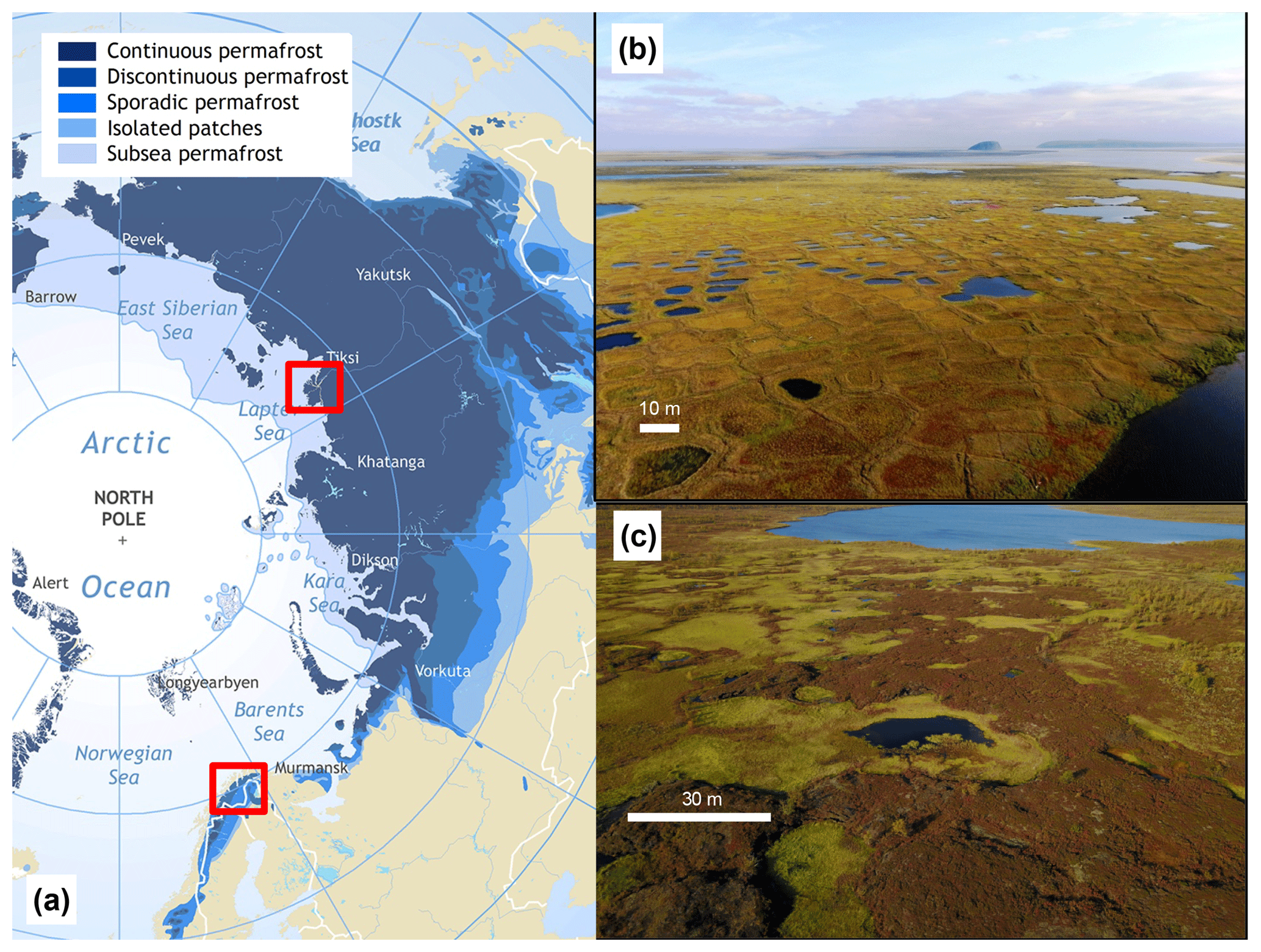
Figure 1 (a) Location of the two test sites on top of the map of permafrost distribution in the Arctic (Brown et al., 1997). (b) Example of low-centered polygons on Samoylov Island, northern Siberia (photo: Sebastian Zubrzycki). (c) Example of peat plateau near Suossjavri, northern Norway (photo: Sebastian Westermann). The two sites are located in the continuous and sporadic permafrost zones.

2.1.1 Samoylov Island, northern Siberia

Samoylov Island (72^∘22^′ N, 126^∘28^′ E) is located in the southeast corner of the Lena River delta. The size of the entire Delta, including more than 1500 islands and about 60 000 lakes, is about 25 000 km² (Fedorova et al., 2015), and the area is underlain by continuous cold permafrost. The island of Samoylov, located in the southern part of the delta, mainly consists of polygonal tundra with a number of ponds and lakes (Fig. 1b; Boike et al., 2013, 2018). All degradation stages described by Liljedahl et al. (2016) can be found here, from non-degraded LCPs to HCPs with connected troughs (see Nitzbon et al., 2018). Between 1997 and 2017, the mean annual air temperature at the island was approximately −12.3 ^∘C, with an annual liquid precipitation of 169 mm and mean end-of-winter snow depth of 0.3 m (Boike et al., 2018). At the depth of zero annual amplitude (20.8 m), the permafrost had warmed from −9.1 ^∘C in 2006 to −7.7 ^∘C in 2017. Numerous studies have been conducted on the island, including investigations of water and surface energy balance (Boike et al., 2008; Langer et al., 2011a, b) and carbon cycling (Knoblauch et al., 2018, 2015). As a well-studied site with available meteorological, soil physical, and hydrological measurements (Boike et al., 2018), it has also been used as a test site for various permafrost modeling studies, including ESM validation and development (Chadburn et al., 2015, 2017; Ekici et al., 2014, 2015).

2.2 Suossjavri, northern Norway

Suossjavri (69^∘23^′ N, 24^∘15^′ E) is situated in the central part of Finnmark county in northern Norway. It is part of the sporadic permafrost zone in northern Fennoscandia (Fig. 1), where permafrost outside mountain regions is confined to palsas and peat plateaus in mires. The site has an elevation of approximately 335 m a.s.l. and covers about 23 ha. It is bordered by the Iesjoka River in the south and the Suossjavri Lake in the east and north and consists of palsas and peat plateaus that rise up to 2 m above the surrounding wet mire. These permafrost features are degrading strongly, having lost approximately 30 % of their area in the last 6 decades (Borge et al., 2017). The largest degradation rates are seen for the smaller palsas and peat plateaus, which have lost almost half of their area in this period, compared to only 15 % aerial loss of the larger peat plateaus.

The mean annual air temperature in the region ranges from −2 to −4 ^∘C, with a summer mean value of 10 ^∘C (JJA) and winter value of −15 ^∘C (DJF; Aune, 1993, for the 1961–1990 period). The mean annual precipitation is below 400 mm according to the nearest measurement station (Borge et al., 2017). Mean annual ground surface temperatures (MAGSTs) have been measured with iButton^® temperature loggers at 25 locations since September 2015, in conjunction with end-of-summer thaw depths and end-of-winter snow depths at the same points. These show snow depths on the peat plateaus mostly between 0 and 40 cm, an active layer thickness (ALT) between 40 and 70 cm, and 1 to 2 ^∘C colder MAGSTs compared to the surrounding wet mire areas.

2.3 The Noah-MP land surface model

The modeling study is performed with the Noah-MP LSM version 3.9, with a number of modifications described below. In its default configuration the Noah-MP model (Niu et al., 2011) simulates soil temperature and frozen and liquid water in four soil layers down to a depth of 2 m. It includes up to three snow layers with a representation of liquid water retention and refreezing, as well as a separate canopy layer. Compared to the original Noah code, Noah-MP is an augmented version that includes multiple alternative model representations for key processes, including parameterizations of supercooled liquid water and frozen ground hydraulic conductivity (see details in Niu et al., 2011). It is substantially less complex and computationally expensive than LSMs used in current state-of-the-art ESMs, lacking for instance representations of biogeochemical processes and dynamical vegetation. However, in its basic treatment of soil thermal and hydrological processes, it is comparable to, and includes some of the same parameterizations as, the Community Land Model (CLM; Lawrence et al., 2011). Furthermore, lateral subsurface water fluxes are already implemented in this model as part of the WRF-Hydro modeling system (see Sect. 2.2.4). With some modifications it is therefore a suitable base model for studying the geophysical aspects of permafrost thaw, including the importance of lateral fluxes. In the following, we will describe the modifications and augmentations to the Noah-MP model for our simulations.

2.3.1 Soil resolution, excess ice, and soil organic fraction

To better represent permafrost processes, the number of soil layers was increased from the default four to 37, with the total soil depth increasing from 2 to 7 or 14 m, plus excess ice thickness (Fig. A1). These soil depths were chosen to approximately include the zero annual amplitude depth at Suossjavri and Samoylov but still be shallow enough to avoid long spin-up times, as the emphasis of this work is on near-surface processes rather than deep soil conditions.

Secondly, we added soil organic fraction as an additional (fixed) input variable. Following Lawrence and Slater (2008), soil thermal and hydraulic properties were calculated assuming a linear weight between organic and the (original) mineral fractions. This facilitated simulating organic rich soils like peat whose properties are different from the default soil types available in Noah-MP.

Following Lee et al. (2014), we included excess ice within the existing layers of the model, so that the layer thicknesses and properties of the layers change throughout the simulation as the excess ice melts. Excess ice is initialized as a certain fraction (F_exice), within a certain depth region in each soil column (see Figs. 3 and A1). Because excess ice is incorporated as an initial condition, it only melts and does not grow. The water from melting excess ice is added to the soil column in the layer where it melts or the nearest unsaturated layer above if this layer is saturated.

2.3.2 Implementation of interacting tiles

Subgrid tiles have been implemented in the original Noah version as part of the Weather Research and Forecasting (WRF) model to represent a mosaic of land cover types (Li et al., 2013). This tiling included soil columns simulated independently for each tile, but without any interaction between the tiles during the simulation. Here we build upon this methodology to explicitly simulate individual land units within a grid cell, but also include lateral fluxes as described below. In the following general description of the interactive tiles, we will refer to these as tiles 1 and 2, but later we refer to them as RIM and CENTER for the polygonal tundra and PPLAT and MIRE for the peat plateau setting (Fig. 2).

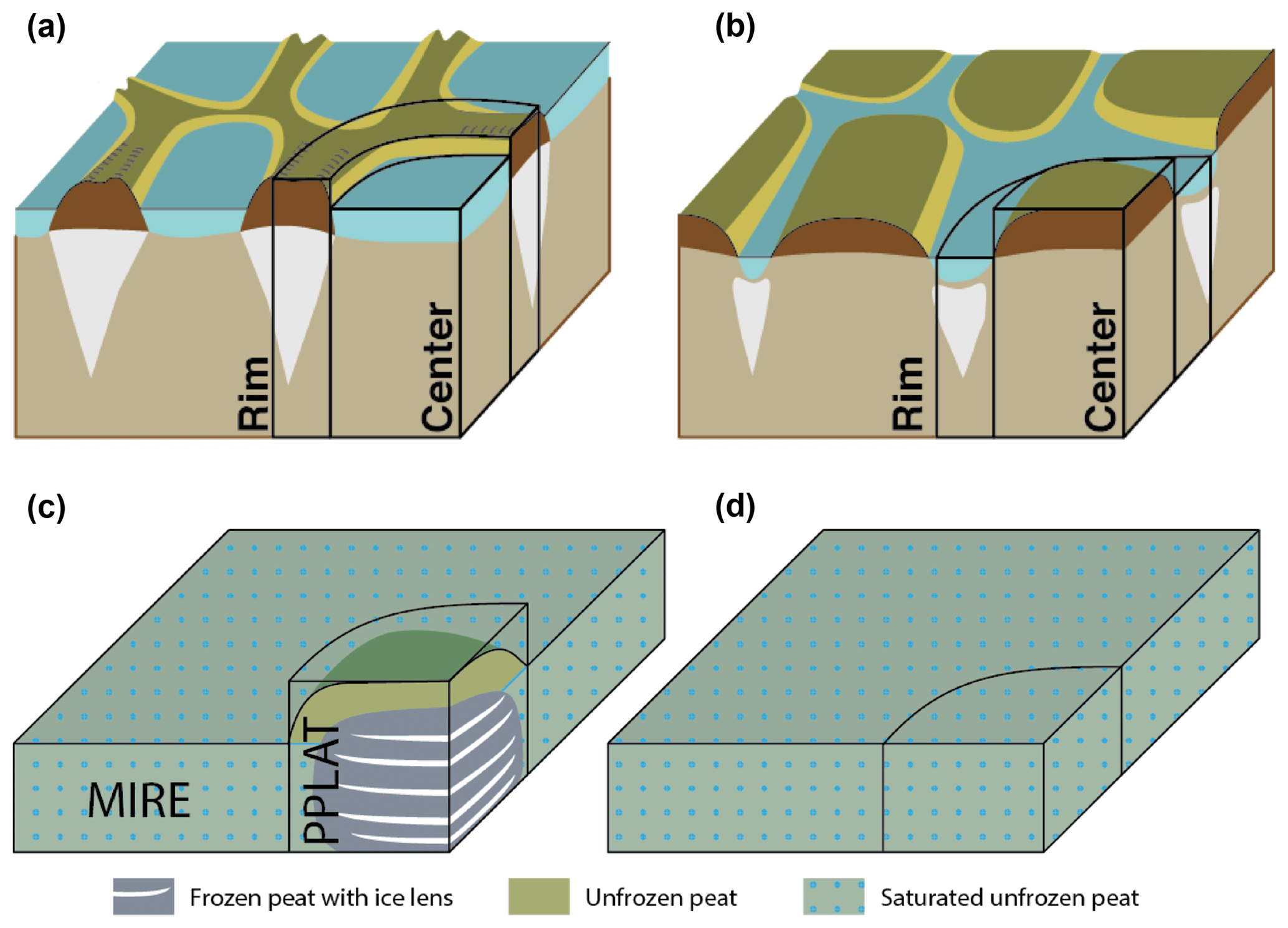
Figure 2 (a) Schematic presentation of non-degraded low-centered polygons (left) and degraded high-centered polygons (right) with corresponding tiles used in this study (adapted from Liljedahl et al., 2016). (b) Schematic presentation of peat plateau in a surrounding mire (left), and the mire after the peat plateau has degraded (right), with corresponding tiles.

2.3.3 Snow redistribution between interactive tiles

To represent the effect of snow redistribution by wind, we scale the amount of snow received in tiles 1 and 2 based on the difference in elevation at the top of the snow or soil column. Similar to Aas et al. (2017), this is performed with a scaling factor, so that the accumulation of snow in tile i is calculated according to the grid-cell mean snowfall S times the scaling factor f_i ($S_i=f_i\cdot S)$.

The scaling factor is calculated as follows: for snow depths below a minimum snow value ($H_{{\mathrm{s}}_{min}}$), no redistribution takes place, i.e.,

$$\begin{array}{}\text{(1)}& {\displaystyle }{f}_i=\mathrm{1.0},\text{for}{H}_{{\mathrm{s}}_i}<H_{{\mathrm{s}}_{min}}.\end{array}$$

Once the tile with the highest elevation reaches the minimum snow value, the scaling factor is calculated so that no new snow accumulates on this tile before the total snow and soil elevation (z_i) are within 5 cm of each other:

$$\begin{array}{}\text{(2)}& {\displaystyle }{f}_{\mathrm{1},\mathrm{2}}=\left\{\begin{array}{lll}\mathrm{1.0},& \text{for}& \left|z_{\mathrm{1}}-z_{\mathrm{2}}\right|<\mathrm{0.05}\mathrm{m}\\ \mathrm{0.0},& \text{for}& \left(z_{\mathrm{1},\mathrm{2}}-z_{\mathrm{2},\mathrm{1}}\right)\ge \mathrm{0.05}\mathrm{m}\\ \mathrm{1.0}+{\displaystyle \frac{A_{\mathrm{2},\mathrm{1}}}{A_{\mathrm{1},\mathrm{2}}}},& \text{for}& \left(z_{\mathrm{2},\mathrm{1}}-z_{\mathrm{1},\mathrm{2}}\right)\ge \mathrm{0.05}\mathrm{m}\end{array}\right.,\end{array}$$

where A refers to the area of the tile, and the subscript refers to the tile number (1 or 2).

2.3.4 Lateral subsurface water flux between interactive tiles

Lateral water flux is calculated similar to subsurface flow in WRF-Hydro (Gochis et al., 2015), with a few modifications relevant for permafrost conditions. The flow rate (m³ s⁻¹) from one tile to another can be calculated as

$$\begin{array}{}\text{(3)}& {\displaystyle }q=\left\{\begin{array}{lll}-T\tan \left(\mathit{\beta }\right)L,& \text{for}& \mathit{\beta }<\mathrm{0}\\ \mathrm{0},& \text{for}& \mathit{\beta }\ge \mathrm{0}\end{array}\right.,\end{array}$$

where T is the transmissivity, L is the contact length, and β is the water table slope between the tiles. T is given by

$$\begin{array}{}\text{(4)}& {\displaystyle }T=\left\{\begin{array}{lll}{\displaystyle \frac{K_{\mathrm{sat},\mathrm{0}}{Z}_{\mathrm{B}}}{n}}{\left(\mathrm{1}-{\displaystyle \frac{z_{\mathrm{wt}}}{Z_{\mathrm{B}}}}\right)}^n,& \text{for}& z_{\mathrm{wt}}\le Z_{\mathrm{B}}\\ \mathrm{0},& \text{for}& z_{\mathrm{wt}}>Z_{\mathrm{B}}\end{array}\right..\end{array}$$

Here z_wt is the water table depth, Z_B is depth to the bottom of the soil column, K_sat, 0 is the saturated hydraulic conductivity at the surface, and n is a tunable local power-law exponent determining the decay rate of K_sat with depth.

Here we set n=1 and use the depth to the minimum (highest) frost table depth (z_frzmin) instead of the full soil depth Z_B. Inserting $\tan \left(\mathit{\beta }\right)=\frac{z_{{\mathrm{wt}}_{\mathrm{1},\mathrm{2}}}-z_{{\mathrm{wt}}_{\mathrm{2},\mathrm{1}}}}{D}$, where D is the distance parameter, the flow rate can then be calculated as

$$\begin{array}{}\text{(5)}& {\displaystyle }{q}_{\mathrm{1},\mathrm{2}}=\left\{\begin{array}{l}-W{K}_{\mathrm{sat}}{\displaystyle \frac{z_{{\mathrm{wt}}_{\mathrm{1},\mathrm{2}}}-z_{{\mathrm{wt}}_{\mathrm{2},\mathrm{1}}}}{D}}\left(z_{\mathrm{frzmin}}-z_{\mathrm{wtmin}}\right),\\ \text{for}{z}_{\mathrm{frzmin}}\ge z_{\mathrm{wtmin}}\\ \mathrm{0},\text{for}{z}_{\mathrm{frzmin}}<z_{\mathrm{wtmin}}\end{array}\right..\end{array}$$

Here we set the frost table to the top of the first layer (from the top) with more than 1 % volumetric soil ice (including excess ice). The water table depth is taken as the depth to the top of the first saturated soil layer.

2.3.5 Lateral heat flux between interactive tiles

The lateral ground heat flux (W m⁻²) between two tiles with overlapping soil depth of Δz can be calculated as (see Langer et al., 2016)

$$\begin{array}{}\text{(6)}& {\displaystyle }q{s}_{\mathrm{1},\mathrm{2}}={\displaystyle \frac{L}{A_{\mathrm{1},\mathrm{2}}}}{k}_{\mathrm{s}}{\displaystyle \frac{T_{\mathrm{2},\mathrm{1}}-T_{\mathrm{1},\mathrm{2}}}{D}}\mathrm{\Delta }z,\end{array}$$

where k_s is the thermal conductivity. This is calculated individually for each partially overlapping soil layer.

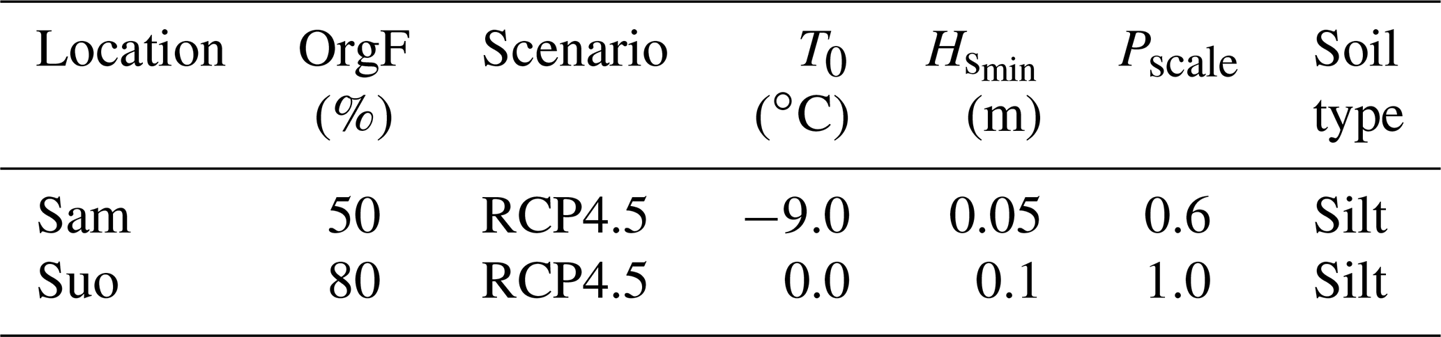
2.4 Model setup and forcing

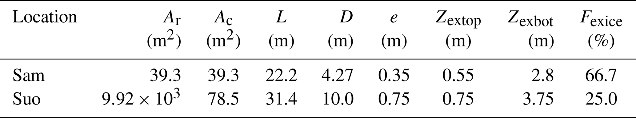
The model setup is shown in Fig. 3 and Tables 1 and 2 and described separately for the two locations in the following, together with the forcing data for the corresponding locations. In both cases, a model time step of 15 min is applied, with zero flux as the lower thermal boundary condition. To represent larger-scale landscapes with a small number of tiles, we exploit the concept of self-similarity (i.e., translational symmetry). At both locations, a separate reference simulation (REF) is run with the same initial conditions as the elevated tile in the laterally coupled system (RIM or PPLAT), corresponding to the same model setup as employed in Lee et al. (2014), i.e., a 1-D excess ice representation without lateral exchange. The other (initially lower) tile in the laterally coupled simulation is referred to as CENTER and MIRE for the tundra and mire locations, respectively.

Table 1 Tile geometry and excess ice distribution. See details in Fig. 3.

Table 2 Soil properties and initial conditions.

2.4.1 Polygonal tundra on Samoylov Island, northern Siberia

The polygonal landscape at Samoylov Island is represented by two tiles that represent center and rim areas. These are in reality different sizes and shapes (Fig. 1) but can to a first approximation be considered a self-repeating pattern, as also described by Nitzbon et al. (2018). Due to symmetry, a larger region can then be represented as a single feature with a representative geometry, neglecting the interaction between different polygons. For simplicity, here we simulate a representative polygon as a circular feature with a center and rim of equal area and a total diameter of 10 m. Assuming hexagons instead of circles, like Nitzbon et al. (2018), would only require minor modifications to the parameters shown in Fig. 3, particularly the distance parameter and the interaction length.

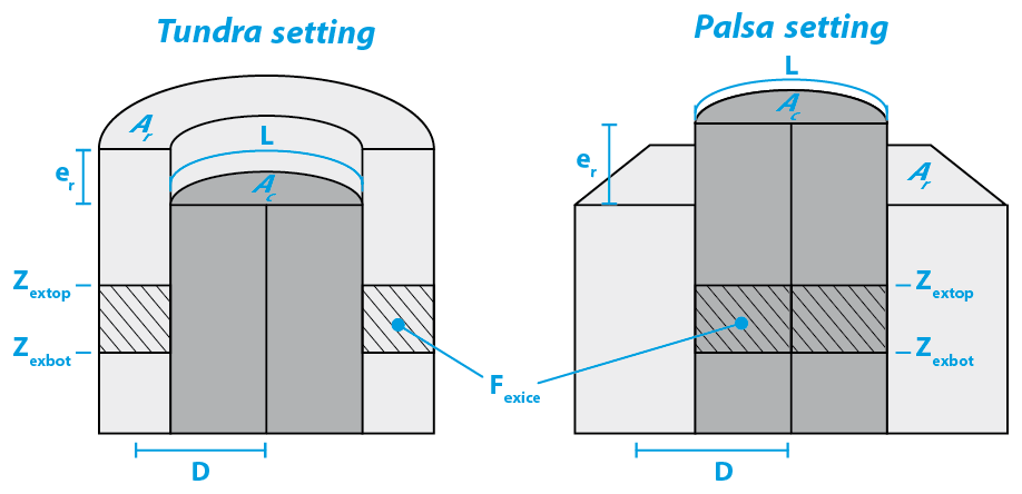
Figure 3 Schematic presentation of the two-tile system with geometry parameters. Parameter values used for the two locations are listed in Table 1.

To represent an ice wedge occupying the majority of the soil volume, we initialize the RIM tile with an excess ice fraction of two-thirds between the simulated ALT at 55 cm and 2.8 m below the surface, which expands the soil thickness of the RIM by 1.5 m. To allow the RIM to sink below the elevation of the center, we add excess ice to the bottom soil layer, with the largest amount in CENTER, so that the total elevation difference is only 35 cm (Fig. A1). This is an approximate average value for observed rim heights at Samoylov. The model is initialized with a soil temperature of −9 ^∘C and fully saturated and frozen soil throughout the column. While this is substantially colder than the equilibrium temperature reached by the model, the soil temperatures in the lowest cell (lower boundary at ca. 16 m, i.e., 14 m plus 2.15–2.5 m excess ice) reach an equilibrium within the first decade of the simulation (mean increase of 0.3 ^∘C yr⁻¹), after which the annual changes vary between positive and negative values.

As model forcing for the Samoylov Island simulation, we used the same model input as Westermann et al. (2016). This is based on the CRU-NCEP data for the historical period (1901–2015; Viovy, 2018). For the future part of the simulation, this dataset uses model output from the CCSM4 climate model following the mitigation scenario RCP4.5, to calculate monthly climate anomalies for temperature, humidity, pressure, and wind and scaling factors for precipitation and radiation. These are added or multiplied to the high-frequency data from 1996 to 2005 from the historical (CRU-NCEP) data, following Koven et al. (2015). The RCP4.5 scenario was chosen as it represents a strong mitigation scenario but still shows continued warming in the Arctic throughout the 21st century, which makes understanding permafrost processes highly relevant.

Detailed measurements of snow accumulation from eight LCPs from 2008 showed average snow depths of 17 cm on the rims and 46 cm in the centers, with a total average snow water equivalent (SWE) of 65 mm (Boike et al., 2013). As the model accumulated too much snow compared to these observations due to a bias in the precipitation forcing (Westermann et al., 2016), we scaled the precipitation with a constant factor (P_scale) of 0.6 throughout the simulation in order to simulate realistic SWE and snow depths.

2.4.2 Peat plateaus in Suossjavri, northern Norway

Similar to the polygonal tundra, the peatland of Suossjavri is represented with two interacting land units. In this case we represent a single circular peat plateau with a diameter of 10 m, corresponding to the smaller features observed in the study area. This is placed in a significantly larger (100 m × 100 m) surrounding mire, so that the effect of the coupling mainly affects the elevated tile. The areas of both the mire and the peat plateau can be increased to represent larger features (see Sect. 4.2), and more complex geometries can be represented by applying appropriate distance and contact length parameters. As the mire does not contain permafrost, only the peat plateau tile (PPLAT) was initiated with excess ice (Fig. A1b), starting 75 cm below the surface with a total excess ice thickness of 75 cm distributed down to 3.75 m below ground. Both tiles were started from fully saturated conditions and 0 ^∘C soil temperatures. The soil water was initially unfrozen in all soil layers, except for the ones containing excess ice, in which soil (pore) water was initially frozen.

Forcing data for this location were generated in a similar way as the data used at Samoylov Island. CRU-NCEP data from the nearest grid point were used for the historical part, while anomalies for the future (starting in year 2010) were taken from CCSM4 simulation following the RCP4.5 scenario and added or multiplied to the reference period 1996–2005.

3 Results

In the following, we outline the model results for the polygonal tundra site in northern Siberia (Sect. 3.1) and the peat plateau location in northern Norway (Sect. 3.2).

3.1 Samoylov Island, northern Siberia

During the simulation period, Samoylov Island experiences a strong increase in annual mean air temperature and a modest increase in precipitation (Fig. 4a). Mean air temperatures increase from approximately −14 ^∘C in the early 20th century to about −8 ^∘C towards the end of the 21st century (RCP4.5 scenario), with most of the warming occurring in the 21st century.

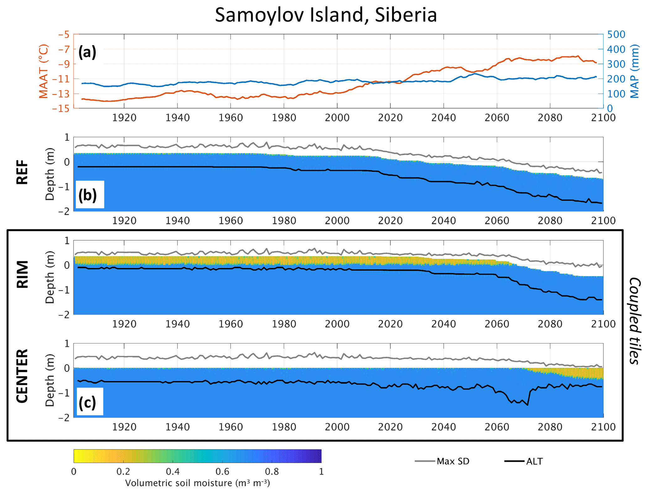
Figure 4 (a) The 10-year running average of mean annual air temperature (MAAT) and mean annual precipitation (MAP) at Samoylov Island. Soil moisture and surface elevation are shown as colored regions in (b) the reference simulation (c) and in the laterally coupled tiles. Note that both the surface elevation (relative to the CENTER tile) and the unsaturated soil (orange and green) change in the coupled tiles as excess ice melts and the lateral fluxes change. Maximum annual snow depth (MaxSD) and active layer thickness (ALT) are shown as gray and black lines, respectively.

Both the reference and the laterally coupled simulations show stable permafrost with ALT between 0.45 and 0.65 m during the historical period of the simulation (until 2010). This is in good agreement with observations, showing mean ALT close to 0.5 m (Boike et al., 2013, 2018). For snow depth and near-surface soil moisture conditions, the laterally coupled simulations show clear differences from REF (Fig. 4b and c) and mimic the observed conditions more closely (see Boike et al., 2013, 2018, and Nitzbon et al., 2018). The simulated maximum snow depths in 2008 compare well with observations for both RIM (0.23 m compared to 0.16 m) and the centers (0.39 m compared to 0.46 m), although the observations show a considerable spread (see Nitzbon et al., 2018). This was partly achieved by applying a scaling factor for precipitation (P_scale) of 0.6 (Table 2). In agreement with observations (see Chadburn et al., 2017, and Nitzbon et al., 2018), the model displays dry near-surface soil conditions in the RIM and mostly saturated conditions in the CENTER tile, which cannot be represented in the REF simulation. With increasing air temperatures in the 21st century, the ALT deepens and surface subsidence occurs in REF, reaching 35 cm around 2030 and more than 1 m by the end of the century. In the two-tile simulation, RIM remains relatively stable and elevated above the center until around 2070, almost 4 decades later than REF. RIM subsequently subsides due to excess ice melt, eventually sinking below CENTER, which marks the transition from LCP to HCP. Towards the end of the simulation RIM appears to stabilize with a subsidence of 80 cm and an ALT of less than 1 m, in contrast to the single-tile REF.

CENTER experiences ALT deepening in the 21st century, which reaches a maximum around 2070. The deepening of the active layer follows the rapid increase in forcing temperature and lasts until RIM has subsided below CENTER. After this point the elevated RIM tile has turned into a trough, and the top layers in CENTER start to drain, resulting in shallower ALT. This marks the transition from a LCP to a HCP.

Soil temperatures. The annual cycle of the soil temperature is shown in Fig. 5. In the current climate (Fig. 5a, c), the elevated rim shows annual temperature variations in the active layer of more than 20 ^∘C, in agreement with observations (Boike et al., 2018). At depth, the soil temperatures are higher than observed, with values of around −3 ^∘C in REF and −5 ^∘C in the laterally coupled simulation, compared to −8.6 ^∘C at 10.7 m in depth observed during the second half of this decade (Boike et al., 2013). Here it is worth noticing, however, that these temperatures have increased more than 1 ^∘C during the last decade (Boike et al., 2018).

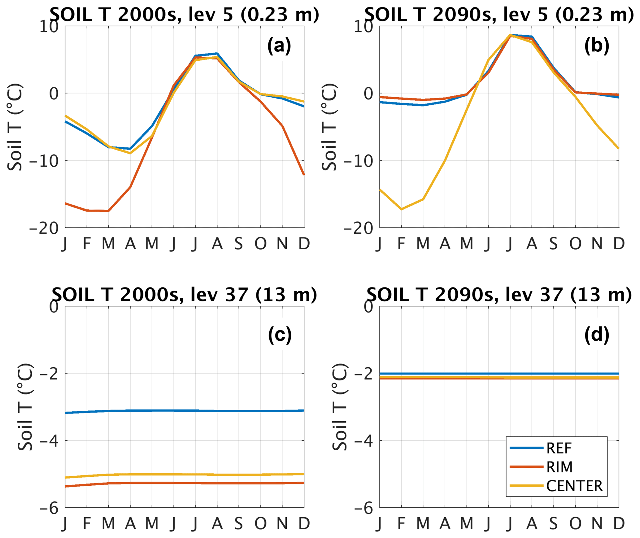
Figure 5 Average annual temperature cycle during the first (a, c) and last (b, d) decades of the 21st century at Samoylov Island, in the fifth model layer (a, b; 0.23 m below surface) and the 37th model layer (c, d; approximately 13 m below reference height). See layer depths in Fig. A1a.

Again, clear differences can be seen between REF and the laterally coupled tile system. In the current climate (Fig. 5a, c), REF and CENTER show a very similar annual cycle, whereas the amplitude of the temperature cycle is much larger in RIM. In the active layer, the difference is almost exclusively observed during winter, when the effect of shallower snow depth is decreasing the winter insulation in RIM. Deeper in the soil column the differences in soil temperature become less pronounced between the two coupled tiles (RIM and CENTER), as heat exchange between the tiles becomes more important. In the deep soil (Fig. 5c) the temperature is similar (within 0.5 ^∘C), but around 2 ^∘C colder than in REF. At the end of the century (Fig. 5b), the situation has reversed and the now elevated, dry CENTER with low snow accumulation features cold winter temperatures, whereas RIM largely follows REF. Deeper in the soil, the two coupled tiles are again colder than REF, although the difference is smaller than in the beginning of the century (Fig. 5d). Comparing the temperatures at 2 m in depth from the surface in REF and the area-weighed mean of the two coupled tiles (here mean of RIM and CENTER), we find the coupled simulation on average 2.1 ^∘C colder than REF during the 20th century. This difference decreases to almost zero during the transition from LCP to HCP, before the coupled simulation becomes 1.4 ^∘C colder during the final 2 decades of the simulation.

Summer surface energy fluxes. A clear difference between the tiles is seen in the summer surface energy fluxes (Fig. 6). As expected, the dry RIM shows larger sensible heat (SH) and lower latent heat (LH) fluxes than REF before degradation, whereas the wet CENTER shows the opposite (Fig. 6a). This is reversed in the degraded state when CENTER is dry and the trough (subsided RIM tile) is wet. Interestingly, the landscape aggregated values (here the mean of RIM and CENTER) is only a few watts per square meter different from the reference for these two fluxes both before and after degradation (Fig. 6a, b). We note, however, that this depends on drainage conditions. Here only surface water (infiltration excess) is removed as runoff, whereas advanced degradation of this kind of polygons is often associated with drainage also of the troughs (Liljedahl et al., 2016). This effect is not included here but is simulated and discussed by Nitzbon et al. (2018) and would likely increase the Bowen ratio of laterally coupled tiles in the degraded stage compared to both REF and the non-degraded stage. It is also likely that the difference between the reference simulation and the aggregated values would be larger with a different areal fraction of RIM compared to CENTER.

Figure 6 Summer surface energy fluxes at Samoylov Island during the first (a) and last (b) decades of the 21st century in the reference simulation (REF) and laterally coupled tiles (RIM and CENTER). SH: sensible heat flux; LH: latent heat flux; GRDFLX: ground heat flux.

The ground heat flux (GRDFLX) is lower during both time periods for the mean of the two coupled tiles than the REF, due to a substantially reduced flux in the dry, elevated tile (first RIM, then CENTER). This points to the effect of dry peat insulating the soil and suggests that the lower temperatures in the laterally coupled system could be a result of both increased summer insulation as well as the reduced winter insulation mentioned above.

Qualitatively, our simulation captures the observed difference between the RIM and CENTER reported by Langer et al. (2011b), although the simulation seems shifted towards higher SH fluxes and lower LH fluxes. This again might be related to too low water holding capacity in our simulations, as well as the lack of surface water on top of the LCP.

3.2 Suossjavri, northern Norway

Figure 7 shows the soil moisture, surface elevation, ALT, and snow depth at the mire location in the sporadic permafrost zone in northern Norway. In REF, permafrost starts to degrade at the beginning of the simulations, with excess ice rapidly disappearing during the first 3–4 decades of the simulation. After this point, REF has turned into a mostly saturated wetland with maximum snow depths of around 1 m. The corresponding tile in the laterally coupled system (PPLAT) experiences low maximum snow depths and dry surface conditions (Fig. 7c), which results in a thermally stable peat plateau throughout the 20th century. Compared to observations at this location (see Sect. 2.1.2), the PPLAT shows a somewhat larger ALT (0.75–0.9 m) in the historical period. The initial excess ice does not start to melt until around 2030, when both air temperatures and precipitation start to increase rapidly. Accelerating ALT deepening in conjunction with surface subsidence due to excess ice melt is seen after 2050, when the mean air temperature has stabilized at about −1 ^∘C and precipitation at around 650 mm. This process appears to be driven by feedbacks in the system: as the ALT deepens and excess ice melts, the peat plateau subsides, leading to more snow remaining in this tile and smaller heat loss during winter, which again enhances summer melt. Furthermore, the subsidence also results in a thinner layer of dry peat as the water table is largely controlled by the elevation relative to the surrounding wet mire, which lowers the insulation during summer. Combined with the direct effect of water from the excess ice melt increasing the soil moisture in PPLAT, this leads to a melt–subsidence–soil moisture feedback, in addition to the melt–subsidence–snow feedback. The surrounding MIRE is largely unaffected by the presence and disappearance of the elevated peat plateau as it is assumed to be about 2 orders of magnitude larger. Hence, REF and MIRE develop very similarly after the initial excess ice in REF has melted.

Figure 7 (a) The 10-year running average of mean annual air temperature (MAAT) and mean annual precipitation (MAP) at Suossjavri, northern Norway. Soil moisture and surface elevation are shown as the colored region in (b) the reference simulation (c) and in the laterally coupled tiles. Note that both the surface elevation (relative to the CENTER tile) and the unsaturated soil (orange and green) change in the coupled tiles as excess ice melts and the lateral fluxes change. Maximum annual snow depth (MaxSD) and active layer thickness (ALT) are shown as gray and black lines, respectively.

Soil temperatures. The soil temperatures in the laterally coupled tiles differ substantially in the present non-degraded state (Fig. 8a, c). While REF and MIRE have nearly identical annual temperature cycles near the surface, PPLAT deviates in several points. First, the elevated PPLAT shows cold winter soil temperatures (as low as −7.6 ^∘C in January), compared to a constant, 0 ^∘C temperature in MIRE and REF. Furthermore, PPLAT responds quicker to the onset of both summer and winter, with both MIRE and REF shifted to warmer temperatures in late summer and colder temperatures during spring. One key factor controlling these differences is the low snow accumulation in PPLAT, which leads to both an increased annual temperature cycle near the surface and earlier snow melt. Another factor is the higher soil moisture in REF and MIRE (both mostly saturated), which due to the high heat capacity of water delays the soil response to changing atmospheric temperatures.

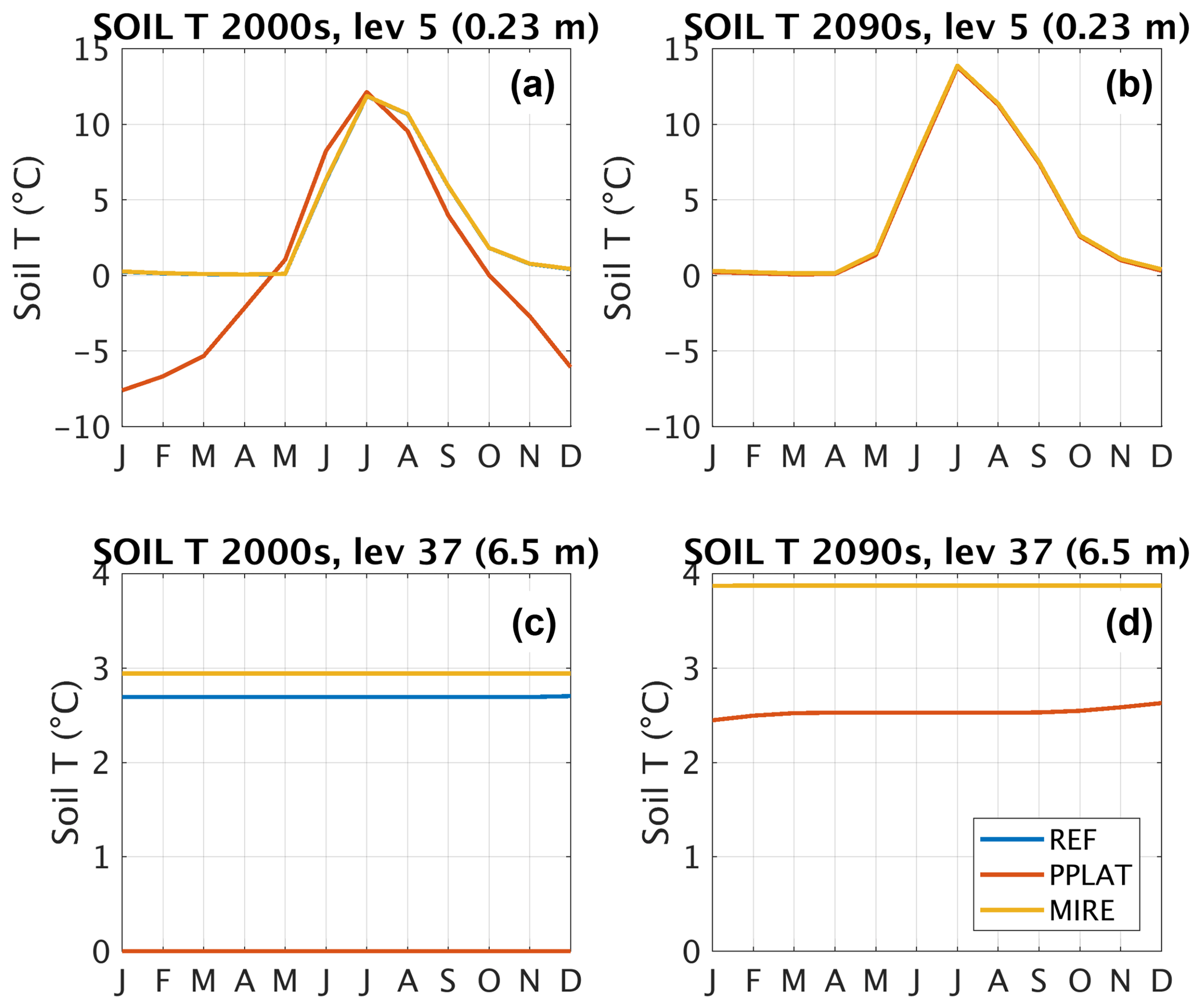
Figure 8 Average annual temperature cycle during the first (a, c) and last (b, d) decades of the 21st century at Suossjavri, northern Norway, in the fifth model layer (a, b; 0.23 m below surface) and the 37th model layer (c, d; 6.5 m below reference height). See layer depths in Fig. A1b.

Below the depth of zero annual amplitude, PPLAT displays warm permafrost conditions at 0 ^∘C, whereas the MIRE and REF feature temperatures close to 3 ^∘C. The REF simulations are about 0.25 ^∘C colder than MIRE, which is most likely a legacy of excess ice melt earlier in the simulation (Fig. 7).

After degradation (Fig. 8b, d), differences among the three realizations are marginal near the surface. At this point, there is no elevation difference, so that differences in snow accumulation and other surface parameters vanish. Some differences remain in deeper soil layers, where the PPLAT tile continues to warm after the ice melt.

Summer surface energy fluxes. The different snow and soil conditions between MIRE and PPLAT are clearly visible in the summer surface energy fluxes (Fig. 9). In the present non-degraded state, the PPLAT tile shows almost opposite SH and LH fluxes compared to both MIRE and REF, which again are practically identical. While the MIRE and REF both show 3 to 4 times larger LH than SH, the opposite is the case for the dry, elevated PPLAT. As the MIRE is 2 orders of magnitude larger than PPLAT in the model setup, the aggregated fluxes are only marginally different from the single MIRE tile (similar to REF). However, observed peat plateaus can occupy a large area of the landscape (as also seen from Fig. 1b), and configurations with larger PPLAT area would likely result in larger differences in the aggregated fluxes.

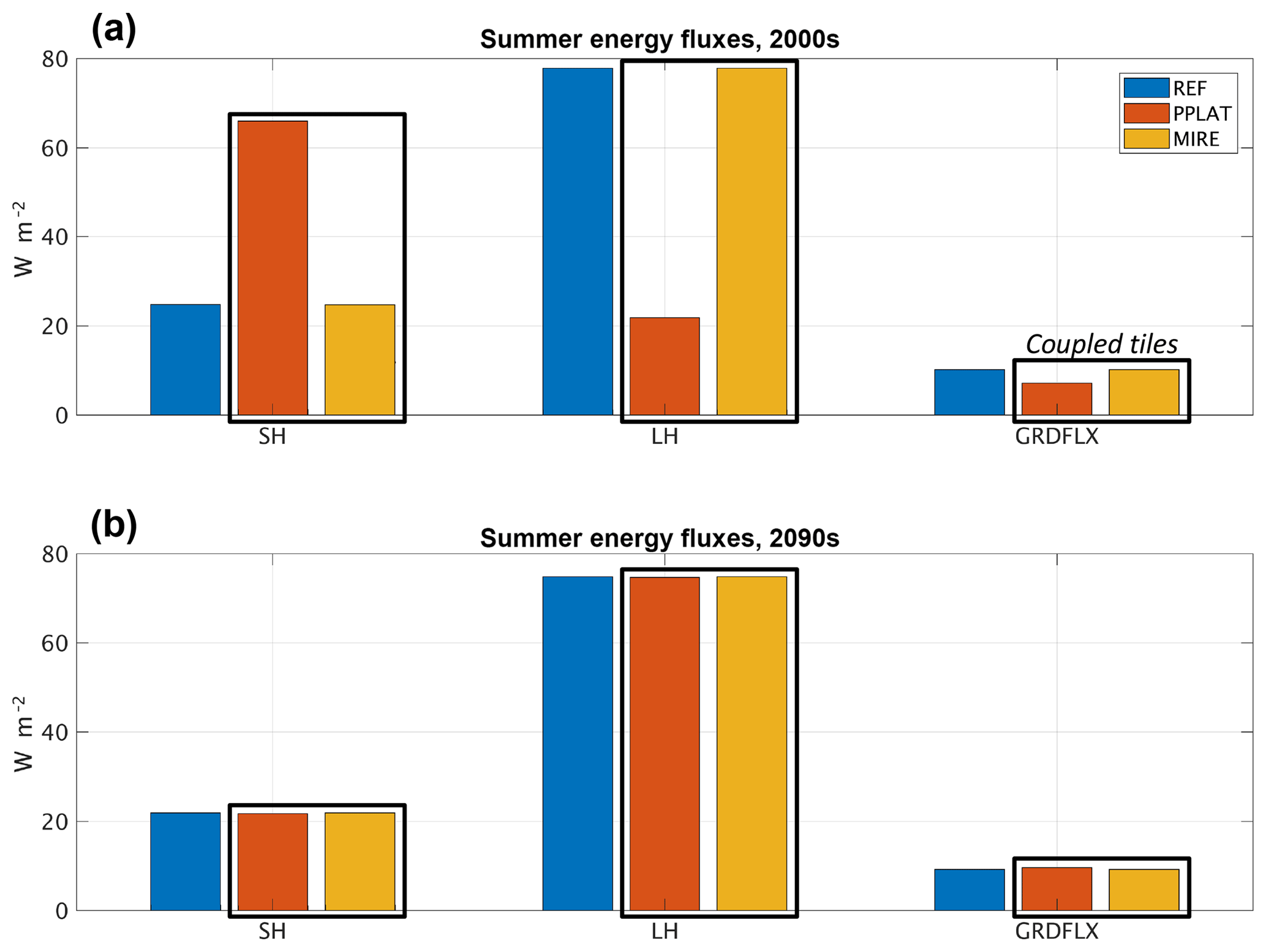
Figure 9 Summer surface energy fluxes at Suossjavri, northern Norway, during the first (a) and last (b) decades of the 21st century in the reference simulation (REF) and laterally coupled tiles (RIM and CENTER). SH: sensible heat flux; LH: latent heat flux; GRDFLX: ground heat flux.

For the ground heat flux (GRDFLX) the differences are smaller, but still substantial. The elevated PPLAT receives on average less energy from the surface during summer compared to both RIM and MIRE. With colder temperatures at depth in this tile, this points to the insulating effect of dry peat, in addition to the abovementioned winter effect due to shallower snow depths. In the degraded phase, the difference among all three realizations has nearly vanished, as the PPLAT is no longer elevated from the MIRE. Here only a slightly larger GRDFLX (barely visible) shows that temperatures in deeper layers have not yet reached an equilibrium.

4 Sensitivity studies

To further investigate the importance of the different processes in the laterally coupled system, we perform two sets of sensitivity studies. First, we look at the effect of selectively activating different lateral fluxes at both locations, before investigating the effect of the distance parameter (D) for the simulation of the peat plateau.

4.1 Snow, water, and heat coupling

Figure 10 shows the surface elevation in the initially elevated tiles (RIM and PPLAT) at both locations for different combinations of lateral fluxes. Here, the thick blue line represents the reference simulation (similar to REF), whereas the simulation with all lateral fluxes activated (similar to RIM and PPLAT) is shown with a thick red line (in the following referred to as “fully coupled”).

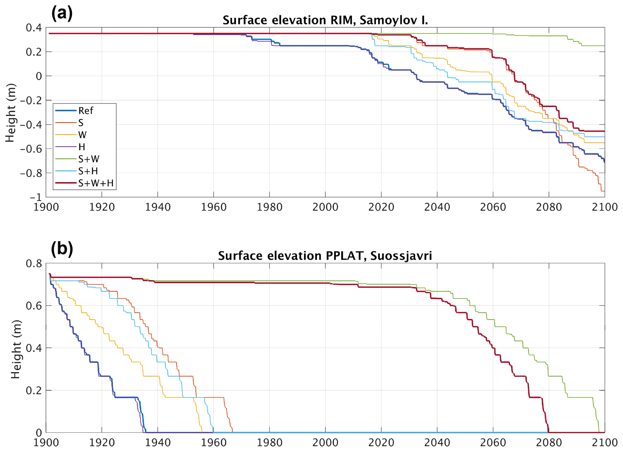
Figure 10 Surface elevation of RIM relative to CENTER at Samoylov Island, Siberia (a), and of PPLAT relative to MIRE at Suossjavri, northern Norway (b), for different combinations of lateral fluxes. The thick blue line represents reference simulations (REF; no lateral fluxes), and thick red line represents the fully coupled two-tile simulation. S: snow; W: water; H: heat.

For the polygonal tundra site (Fig. 10a) the snow effect alone (thin red) gives results similar to those of the fully coupled simulation during most of the time period. The difference is clear only towards the end, when the snow-only experiment continues to melt and subside with a trough approaching 1 m in depth (corresponding to 1.35 m subsidence), while the fully coupled system stabilizes with a 45 cm trough. Adding lateral water (yellow) or heat (purple) fluxes has opposite effects, decreasing and increasing the melting, respectively. The snow-plus-water coupling (green) results in an almost stable rim throughout the simulation, subsiding only about 10 cm before the end of the 21st century, whereas the snow-plus-heat coupling (thin blue line) results in subsidence about 10 years earlier than the fully coupled realization, but eventually stabilizing at almost the same depth.

At the peat plateau location in northern Norway, the combined effect of snow and water coupling is needed to simulate a stable peat plateau throughout the 20th century (Fig. 10b). Only the fully coupled (thick red line) and the snow-plus-water coupling (green) can represent stable permafrost, whereas all other simulations display degradation starting within the first decades of the 20th century and ground ice disappearing entirely before 1970. This is in agreement with previous studies of palsas and peat plateaus in this region, pointing to low snow accumulation and dry peat during summer as the most important factors for their stability (see Seppäla, 2011). Adding the lateral heat flux to the reference setup (purple) has little effect. However, in combination with the snow and water coupling, the heat flux speeds up the melt, so that the peat plateau disappears 2 decades earlier than in the simulations without lateral heat fluxes.

In conclusion, it appears that all three lateral fluxes are important at both locations. Compared only to the reference simulation, the effect of snow redistribution is largest, followed by the effect of coupling through water fluxes, while the effect of the lateral heat flux alone is marginal. However, both snow and water coupling act to cool the elevated tile compared to CENTER and MIRE, as seen by the delayed subsidence. Hence, an increased thermal gradient between the different tiles is generated, which increases the effect of the lateral heat flux, reducing the stabilizing effect of snow and water fluxes and speeding up degradation. The relative effect of the different processes is therefore complex and must be seen in combination with the other fluxes.

The influence of the different lateral fluxes is sensitive to process implementation and key model parameters. This is especially the case for snow redistribution, which in our simulations was found to be the most important lateral process. Here, we redistribute all solid precipitation from the tile with the highest surface elevation (soil + snow), once a minimum snow depth is reached ($H_{{\mathrm{s}}_{min}}$). Increasing (decreasing) this limit will decrease (increase) the effect of snow redistribution in the simulation. An additional set of sensitivity simulations with different values of $H_{{\mathrm{s}}_{min}}$ ranging from 0.0 to 0.15 m (not shown) revealed that the landscape evolution at the polygonal site was relatively insensitive to this value, with the transition from LCP to HCP shifting by less than 2 decades between the minimum and maximum value. A larger sensitivity was seen for the peat plateau site, for which the lowest values of $H_{{\mathrm{s}}_{min}}$ resulted in stable permafrost throughout the 21st century. Similarly, the thermal and hydraulic conductivity of the soil determines the effect of the heat and water fluxes, respectively. However, the effect of lateral heat flux was only important in combination with snow and/or water coupling, as there must already be a thermal gradient between the tiles before it can have an effect.

4.2 Distance parameter (D)

At the peat plateau location, we performed a sensitivity analysis of the distance parameter (D), which determines lateral water and heat fluxes are inversely proportional (Eqs. 5 and 6). However, the water can potentially drain fast, with soil water contents quickly reaching equilibrium, while the heat conduction is generally much slower. To test a wide range of parameter values, we again simulate a circular elevated tile (as in Sect. 3) but scale both the elevated PPLAT and the surrounding MIRE by a factor of 100 in each horizontal direction, testing length scales from 0.2 to 500 m.

Figure 11 shows the resulting surface elevation in the peat plateau (a), as well as the lateral heat (b) and water fluxes (c) shown as 10-year running averages. Here we see that for the most part larger distance parameters correspond to earlier permafrost thaw and ground subsidence. This is clearly a water effect, as the simulated annual horizontal heat flux (HHF) is small (scaling almost linearly with D⁻¹) and snow redistribution does not depend on this parameter. Hence the main mechanism appears to be that larger D leads to lower lateral water fluxes and hence a higher soil moisture and larger soil thermal conductivity at PPLAT. Only with very small or large D is this picture reversed. Increasing the distance parameter from 0.2 to 0.5 m instead results in a slight delay in degradation, as the changes in lateral heat fluxes become important for such small values of D, while water redistribution occurs almost instantaneously and does not change noticeably so that larger values of D lead to a slower degradation. On the other end of the simulated range, degradation is also delayed when increasing D from 50 to 100 m and further to 500 m. In these cases, the drainage is much slower, so that full drainage on the annual timescale is no longer realized. Therefore, other processes like the higher heat capacity due to increased soil moisture might be more important than the conductivity effect of reduced drainage.

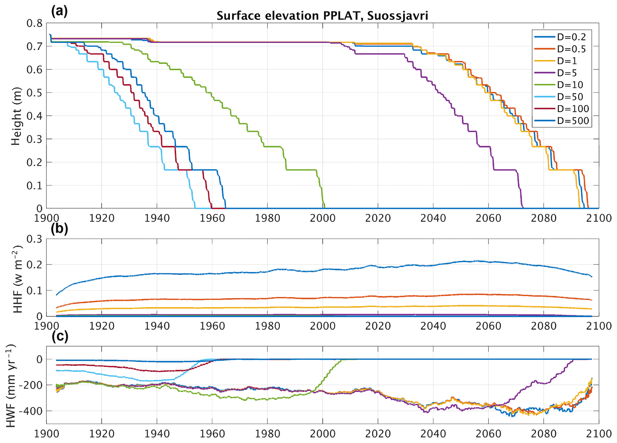
Figure 11 Surface elevation of PPLAT at Suossjavri, northern Norway (a), for different values of distance parameter (D) between the two interacting tiles, and corresponding horizontal heat flux (HHF; b) and horizontal water flux (HWF; c). Note that the area of PPLAT is different (larger) here than in the standard simulations (Fig. 7), giving a different evolution for the same (D=10) distance parameter.

This sensitivity analysis highlights the importance of different lateral fluxes on different scales, suggesting that the effect of laterally coupled tiles strongly depends on the geometries and sizes of the landscape structures represented.

5 Discussion

With a relatively simple two-tile system, we have been able to simulate observed microtopographic changes associated with degradation of ice-rich permafrost. The introduction of laterally coupled tiles influenced the mean soil temperatures, active layer thicknesses, timing of permafrost degradation, soil moisture conditions, and the surface energy balance fluxes. In the following, we discuss limitations and sources of errors in the current study (Sect. 5.1), implementation in large-scale models (Sect. 5.2), and possible implications for simulating the PCF (Sect. 5.3).

5.1 Limitations and sources of errors

The method applied here is by design a minimalist approach to include important lateral processes in permafrost landscapes, keeping the number of new parameters (see Fig. 3) at a minimum. As capturing the detailed properties at the two test locations has not been the objective of this study, the different model parameters have not been fine-tuned, for either the default Noah-MP model or the new tile geometry parameters. As noted in Sect. 3, there are differences between simulations and observations for both locations. In particular, the simulations showed considerably warmer permafrost temperatures and a larger Bowen ratio at Samoylov Island, while the peat plateau at Suossjavri appears more stable in the simulations compared to observations (Borge et al., 2017). In the following, we discuss aspects of the two-tile system that were found to be particularly important for our simulations, as well as processes ignored in the model setup, which might explain some of the discrepancies. However, given the relatively coarse resolution of the forcing data, a certain disagreement must be expected.

Snow. The minimum snow depth ($H_{{\mathrm{s}}_{min}}$) was found to be a key parameter. As seen in Fig. 10, the timing of the degradation at both locations was sensitive to the snow redistribution. This was further confirmed with the sensitivity simulations exploring different $H_{{\mathrm{s}}_{min}}$ values and is in agreement with previous studies on the effect of the seasonal snow cover on the thermal regime (e.g., Gisnås et al., 2016). In our simulations, a higher minimum snow accumulation limit was needed for the peat plateau (10 cm) than for the polygonal site (5 cm) in order to simulate stable conditions in the beginning of the simulation and degradation within the current century. We note that the end-of-winter snow depths at both locations are within the observed range and that the $H_{{\mathrm{s}}_{min}}$ values mainly affect the timing of initial permafrost thaw. In the future, this value should ideally be linked to surface characteristics, such as the vegetation height.

Excess ice initialization. Another key aspect of the two-tile system is how the excess ice is initialized, in particular the depth at which the excess ice is inserted in the soil column (Z_extop). Test simulations revealed that inserting the excess ice at too large or too shallow depths results in a too stable or too dynamic system, respectively. Setting Z_extop to the depth of the simulated ALT was found to produce reasonable results, while inserting the excess ice below the observed ALT resulted in immediate excess ground ice melt, as the ALT was overestimated for both locations (Sect. 3). Likewise, the volumetric fraction of the excess ground ice is important for how fast the system evolves once degradation starts. At the polygonal tundra site, this in particular determines the new stable state after excess ice thaw in RIM, as it determines how fast an excess ice-free buffer layer can form. The values used in the simulations are to some extent based on observations and expert judgement, but still a certain degree of trial and error was needed, in particular to simulate a stable trough at the tundra site without a continued unrealistic deepening of the RIM tile.

Soil properties. An important limitation in the current model system is the uniform soil properties, with respect to both depth and between the tiles. This is a simplification inherent in the current Noah-MP model, which does not consider different soil types at different depths, including our implementation of organic fractions. This meant that in order to represent observed soil properties near the surface, in particular the high porosity typical for peat, we likely had to accept too large porosities deeper in the soil. As a consequence, too much soil water undergoes a phase change at the bottom of the active layer, damping the temperature signal from the surface. In addition, as the initial amount of soil (pore) ice is too large, too much energy might be needed to thaw the soil. Furthermore, formation of new excess ice, as well as explicit representation of surface water above the soil column is not represented in the model. While appropriate model formulations are lacking for the former, the latter has been accounted for in a companion paper (Nitzbon et al., 2018) using a more dedicated permafrost model.

Larger-scale hydrology. As shown in Nitzbon et al. (2018), the hydrological setting within the larger-scale drainage regime is important for the stability of permafrost in polygonal tundra. In this study, surface water is removed as runoff, which corresponds to a single (possible rather artificial) hydrological setting. Observations from Samoylov Island reveal that very different hydrological conditions can be found even on this relatively small island. Simulating surface water in LCPs, or water-filled troughs in the degraded high-centered stage, would likely modify the results through reduced albedo, increased heat conduction, and lower snow redistribution due to smaller elevation differences between the tiles. Results from model simulations, which take larger-scale hydrology into account, show increased soil ALT and earlier permafrost degradation when standing water is included (Langer et al., 2016; Nitzbon et al., 2018).

Vegetation. Another factor not considered in this study is the influence of vegetation. In particular, the appearance of new vegetation in troughs is likely to lead to an increased insulation and act as a negative feedback to the degradation of the polygons, while also interacting with the local hydrology.

Other lateral processes. Finally, there are other lateral processes not accounted for, such as lateral erosion and heat advection associated with lateral water flow. Lateral erosion is a complex process, which likely requires accounting for the heat input along the (vertical or inclined) erosion surface, which cannot be included in the presented model scheme in a straightforward fashion. Furthermore, our simulation only includes lateral water flux near the surface, while a number of studies have demonstrated that deeper water movement and related heat advection might affect soil thermal conditions (Kurylyk et al., 2016; Sjöberg et al., 2016). Both of these processes might play a role in the degradation of peat plateaus currently observed in northern Norway.

Despite these limitations, our results suggest a major improvement in terms of representing current permafrost conditions at the two locations, with discrepancies with in situ observations consistently smaller for the laterally coupled simulation compared to REF. Considering the documented spatial variability in the permafrost ground thermal regime, we consider these differences to be modest, mainly influencing the timing of the future permafrost degradation. Nevertheless, adding further key processes to the two-tile system is likely to improve the simulation results. Here, we consider the representation of standing water as the most important process, followed by representation of vertically varying organic fractions and soil types, as well as dynamical vegetation. Most of these are already included in several large-scale LSMs (e.g., Lawrence et al., 2011; Reick et al., 2013).

5.2 Interactive tiling in coupled ESM simulations?

In this study, we have used Noah-MP as a test model, in which the representation of subsurface processes is comparable to LSMs used for global climate simulations. In a companion study, Nitzbon et al. (2018) demonstrated that the same basic method can be utilized in a completely different model, which suggests that the method is independent of the individual model setup. Implementation in a large-scale LSM, also with full biogeochemistry, should therefore rather be a technical than a conceptual challenge, as is applying the modified model online in an ESM framework. From the theoretical side, the challenge is mainly the scale gap between the small-scale units considered here (on the order of 10–100 m) to the 100 km scale typical for current global simulations. However, as mentioned in Sect. 2.3, the concept of self-similarity offers the possibility to represent larger landscapes with a small set of laterally coupled units.

As the simplest implementation, the two-tile structure outlined in this study could represent a fraction of a grid cell in a large-scale model, alongside the default LSM simulation. Using for instance the maps from Olefeldt et al. (2016), areas of ice-rich permafrost could be represented by a separate land unit consisting of two laterally coupled tiles. Ground ice data from Brown et al. (1997) could provide a starting point here, similar to the study by Lee et al. (2014). Assigning excess ground ice to the first soil layers below the simulated ALT has been a reasonable first-order choice for the two test sites, but this procedure is likely not adequate for areas with excess ice well below the current active layer, e.g., due to burial or melting of excess ground ice in the past (e.g., truncated ice wedges; Brown, 1967). Ultimately, new global datasets for ground ice depth, excess ice density, and geometries of the two tiles must be compiled, for example building on approaches as in Hugelius et al. (2014) and Strauss et al. (2017). Nevertheless, even with relatively crude estimates of these parameters, the proposed method would for the first time allow the inclusion of the effects of lateral heat, moisture, and snow fluxes on permafrost degradation in global models. As suggested by field observations (Liljedahl et al., 2016), these can have substantial effects on the evolution of the permafrost region, which cannot be represented when assuming homogeneous permafrost and ice distributions.

The method described here is, however, not limited to a two-tile structure. As demonstrated by Nitzbon et al. (2018), the same basic formulation can also be applied with three tiles, and with water exchange with an external reservoir. In such a configuration, the coupling method already gives a substantially higher level of realism for the specific site studied (Samoylov Island), although the number of input parameters is correspondingly increased. From a system with three coupled tiles, one could expand the method further to more coupled tiles representing physical locations in a single system (like surrounding hills or waterbodies), or to an ensemble of two- or three-tile systems with different geometries within a single grid cell. However, with the computational cost of current LSMs used in ESMs, this is likely to become a large computational burden. Regardless of the choice of implementation, the method proposed here should be considered in the context of a larger effort to improve the representation of horizontal land processes in ESMs. The land component of coupled atmosphere–land surface models is typically of considerable complexity in the vertical dimension, but includes little horizontal interaction and variation (see, e.g., Clark et al., 2015). While representing heterogeneous excess ice is relevant only in certain regions, we believe that a more flexible model structure with individual subgrid soil columns that can exchange water and snow is a concept that also deserves further investigation in other regions.

5.3 Interactive tiling to improve simulations of future permafrost–carbon feedback?

Improved representation of the PCF is a key motivation for the model developments in this study. In the following, we discuss the prospects of a coupled tile structure in LSMs with respect to simulations of carbon turnover in permafrost regions.

As a first order effect, the PCF depends on how much, and at what time, currently frozen ground is thawed and soil carbon is exposed to microbial decomposition. As substantial changes in permafrost state (e.g., Fig. 5) and timing of degradation (Figs. 4 and 7) have been demonstrated here, it is clear that the simulated PCF is also likely affected by implementing this method in a fully coupled ESM. The CMIP5 ensemble of climate models showed drastically different permafrost areas (Koven et al., 2013a), which have been a major contribution to the uncertainty in the PCF. More recent simulations with improved ESMs (McGuire et al., 2018) still show significant differences in simulated PCF and vegetation response in the permafrost region, despite the fact that they all lack a representation of subgrid processes. Our results therefore suggest that the lack of lateral processes in current large-scale LSMs could potentially contribute to biases in the permafrost area and timing of thawing (e.g., Rowland et al., 2016).

Furthermore, our method shows a nonlinear behavior and thresholds that are not found in the reference simulation. Both the polygonal tundra and peat plateau settings display stable conditions when lateral fluxes are included, before relatively rapid changes are initiated. One reason for this is the nonlinear effect of the snow cover on the insulation of the ground during winter. When considering a grid-cell-averaged snow depth, the effect of slightly increased or decreased snow accumulation is generally small. However, in a laterally coupled system in which snow redistribution depends on dynamical microtopography, even a small increase in snow accumulation can be enough to trigger a change. Once elevated features begin to degrade, more snow begins to accumulate, so that the changes cannot be reversed and may not stabilize before reaching a new state, even if the initial changes in snow accumulation were temporary. This irreversible behavior should be investigated in more detail for so-called overshoot scenarios which are discussed in the context of more ambitious mitigation scenarios (Comyn-Platt et al., 2018).

Accurate simulation of the PCF also depends on the soil moisture conditions under which permafrost thaws and carbon is mobilized. This has been demonstrated in both laboratory studies (Elberling et al., 2013; Schädel et al., 2016; Knoblauch et al., 2018) and model simulations (Lawrence et al., 2015), showing that a realistic simulation of local hydrology is important for PCF simulation. Our results here capture key soil moisture conditions observed in the two simulated permafrost landscapes, which cannot be represented in the reference simulation. Furthermore, our method simulates the rapid transitions in soil moisture conditions that are associated with thermokarst development, which might in itself be an important factor for the amount and partitioning (CO₂ vs. CH₄) of carbon release to the atmosphere. Incubation experiments have shown that the largest greenhouse gas production from thawing permafrost could be realized when previously wet soil was decomposed under drained conditions (Elberling et al., 2013). This is exactly the process observed in the centers when LCPs transition to HCPs, which again suggests that the processes included here might play an important role in simulating permafrost carbon turnover.

Finally, laterally coupled tiling will likely impact dynamical vegetation modeling in the permafrost region, which is important for understanding the future carbon signal from this region. Both greening and browning of the Arctic have been observed in the recent past, although models predict a general greening and increased carbon storage in vegetation (McGuire et al., 2018). Representing subgrid variability in snow and soil conditions in conjunction with a dynamical vegetation model might contribute to simulating future vegetation changes more accurately, e.g., by representing frost damage at locations with shallow snow cover (Phoenix and Bjerke, 2016). This further exemplifies the potential of laterally coupled tiling for simulating land–atmosphere interactions in the Arctic permafrost region in a more realistic fashion.

6 Conclusions

In this study, we simulate dynamically changing microtopography and related lateral fluxes of snow, water, and heat in permafrost landscapes using a two-tile model approach. The model is tested for polygonal tundra in the continuous and peat plateaus in the sporadic permafrost zone, representing two highly different permafrost landscapes dominated by ice-rich ground. The main findings of our investigation are as follows.

1. Currently observed degradation processes in both polygonal tundra and peat plateaus could be simulated with a simple tiling approach accounting for changing microtopography and small-scale lateral fluxes. This included representing the transition from low- to high-centered polygons and the transition from a stable to degrading peat plateau in the sporadic permafrost zone.

2. The timing and speed of degradation at the polygonal site differed strongly between the two-tile model and reference simulations with a classic model using only a single tile. Whereas the reference simulation showed slow but consistent degradation, the laterally coupled tiles showed a delayed onset of permafrost degradation, followed by a more rapid ice melt and subsidence, before the system stabilized in a new state with an elevated dry center and wet trough.

3. Deep soil temperatures differed substantially between the reference simulation and the two-tile system. For the polygonal tundra site, simulated temperatures at approximately 13 m in depth were about 2 ^∘C colder with coupled tiles compared to the reference simulation.

4. The two-tile model was capable of representing dry near-surface soil conditions in the elevated features at both locations, with a substantial effect on surface energy balance fluxes.

5. Sensitivity studies showed that lateral fluxes of snow, water, and heat all affected the stability of the permafrost at both locations, with their relative contribution depending on the distance parameter.

These results show that lateral fluxes and changing microtopography have a strong impact on simulated permafrost extent and conditions. Together with a companion study by Nitzbon et al. (2018), we demonstrate that laterally coupled tiles facilitate a simple and computationally effective first-order representation for a range of observed degradation processes in ice-rich permafrost areas. Applying the proposed method in land surface models with full biogeochemistry shows significant potential to drive simulations of the permafrost–carbon feedback towards reality.

Appendix A

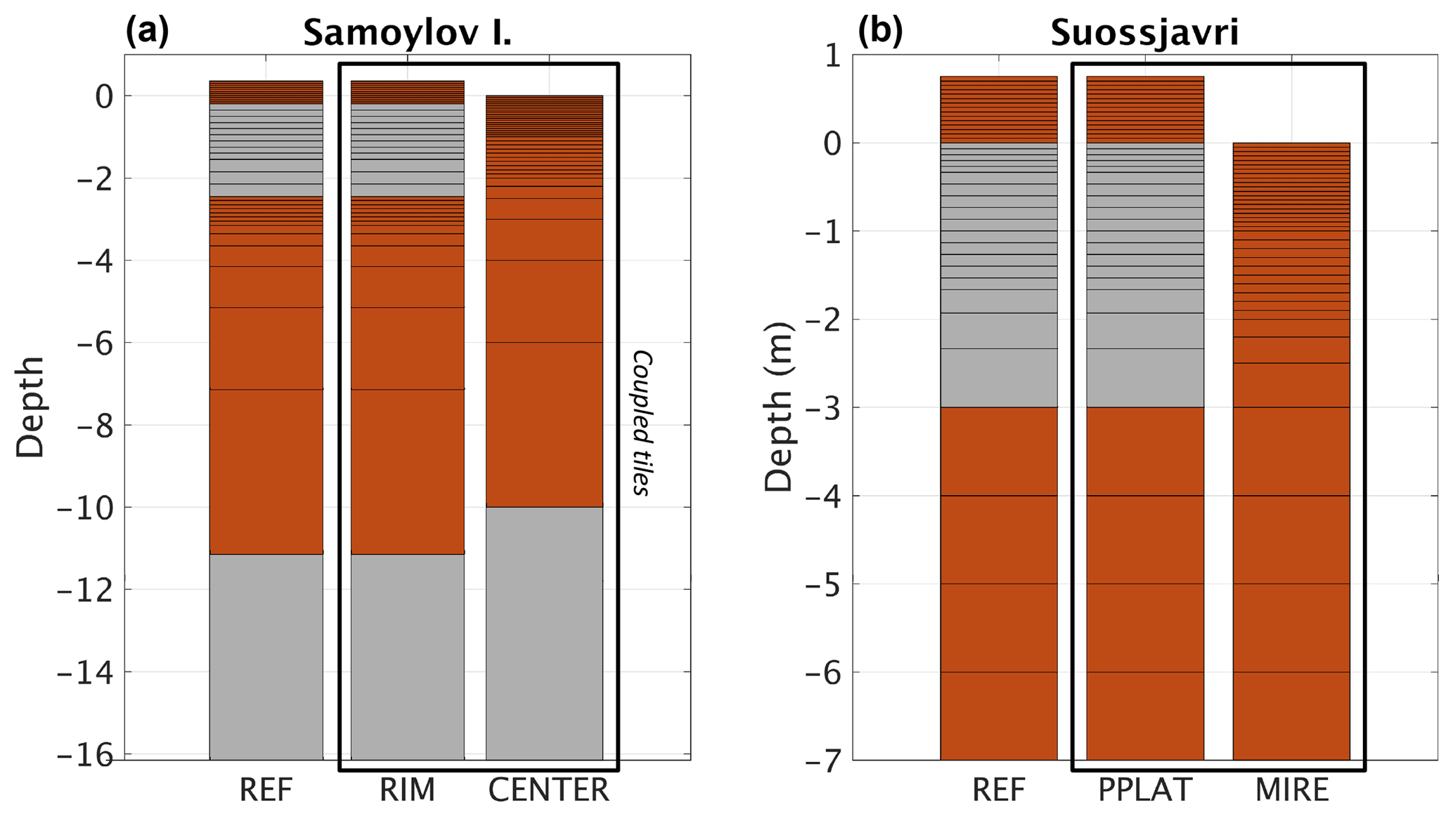
Figure A1 Vertical resolution at Samoylov Island (a) and Suossjavri (b). Gray colors indicate layers initialized with excess ice. Excess ice initiated in the bottom layer at Samoylov Island is used to adjust the rim height (e_r) independently of near-surface excess ice.