the Creative Commons Attribution 4.0 License.
the Creative Commons Attribution 4.0 License.
 | 18 Feb 2019
Assessment of altimetry using ground-based GPS data from the 88S Traverse, Antarctica, in support of ICESat-2
Thomas A. Neumann
Christopher F. Larsen
We conducted a 750 km kinematic GPS survey, referred to as the 88S Traverse, based out of South Pole Station, Antarctica, between December 2017 and January 2018. This ground-based survey was designed to validate spaceborne altimetry and airborne altimetry developed at NASA. The 88S Traverse intersects 20 % of the ICESat-2 satellite orbits on a route that has been flown by two different Operation IceBridge airborne laser altimeters: the Airborne Topographic Mapper (ATM; 26 October 2014) and the University of Alaska Fairbanks (UAF) Lidar (30 November and 3 December 2017). Here we present an overview of the ground-based GPS data quality and a quantitative assessment of the airborne laser altimetry over a flat section of the ice sheet interior. Results indicate that the GPS data are internally consistent (1.1±4.1 cm). Relative to the ground-based 88S Traverse data, the elevation biases for ATM and the UAF lidar range from −9.5 to 3.6 cm, while surface measurement precisions are equal to or better than 14.1 cm. These results suggest that the ground-based GPS data and airborne altimetry data are appropriate for the validation of ICESat-2 surface elevation data.
- Article
(7034 KB) - Full-text XML
-
Supplement
(91152 KB) - BibTeX
- EndNote


The Ice, Cloud, and land Elevation Satellite-2 (ICESat-2) is a next-generation laser altimeter developed by the National Aeronautics and Space Administration (NASA) and launched on 15 September 2018 (Markus et al., 2017). ICESat-2 will carry a single instrument, the Advanced Topographic Laser Altimeter System (ATLAS), a six-beam photon-counting system using <2 ns, 532 nm wavelength pulses with a 10 kHz repetition rate. ICESat-2 will continue NASA's multidecade effort to measure changes in the polar regions (Markus et al., 2017; Webb et al., 2012; Zwally et al., 2011), with mission requirements that include the determination of the annual ice sheet elevation change rates to an accuracy of less than or equal to 0.4 cm a−1 (Markus et al., 2017).
Plans for the post-launch validation of ICESat-2 elevation data products include utilizing both ground-based and airborne elevation datasets. The relatively short ground-based datasets, such as presented here, will provide error assessments for airborne surveys, such that longer airborne surveys can then be designed with sufficient length scales to provide the data volume required for meaningful statistics of satellite data validation. The ground-based activities include the kinematic GPS validation efforts at Summit Station, Greenland (Brunt et al., 2017), and airborne activities, such as those associated with NASA's Operation IceBridge (OIB; Koenig et al., 2010), which includes a lidar as part of the instrument suite.
In support of the ground-based component of ICESat-2 data validation, we conducted a 750 km traverse based out of South Pole Station (Fig. 1), referred to as the 88S Traverse (28 December 2017–10 January 2018). Kinematic GPS data collected along this traverse were used to validate airborne data and will ultimately be used for validation of ICESat-2's spaceborne datasets.
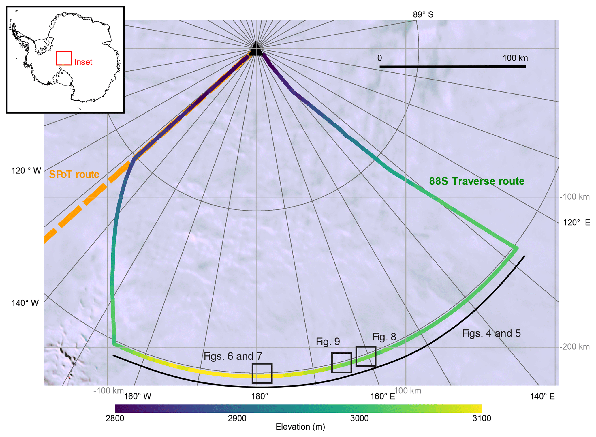
Figure 1Map of the 88S Traverse route, color coded based on elevation. Locations for Figs. 4–9 are also shown. The South Pole Operational Traverse (SPoT) route is indicated in orange. Background is the Landsat image mosaic of Antarctica (LIMA; Bindschadler et al., 2008).
ICESat-2 will have 1387 unique orbits over a 91-day orbital cycle (i.e., all 1387 unique tracks are sampled every 91 days, or four times per year). The orbit has an inclination of 92∘, allowing for data collection between 88∘ north and south. Since ICESat-2 is a six-beam instrument, we refer to the imaginary centerline of the beam pattern as the reference ground track for each of the 1387 tracks. The 88S Traverse was designed specifically to include 300 km of data along the 88∘ S line of latitude, which is the latitude limit of ICESat-2 and where the ICESat-2 reference ground tracks will converge. This 300 km traverse along 88∘ S represents 20 % of the total length of this line of latitude; the traverse route will therefore intersect 20 % (277) of the 1387 ICESat-2 reference ground tracks. Because of Earth rotation, time-sequential ground tracks are not geographically sequentially spaced along the 88∘ S line of latitude. Therefore, the 20 % of the 1387 unique tracks intersected by this survey represent data collected from the whole 91-day orbital cycle, and not a specific 20 % of the cycle. Further, since the ground tracks intersected by the 88S Traverse are spread throughout the 91-day orbital cycle, data from the 88S Traverse mitigate weather limitations (i.e., cloud cover) that have had an impact on other validation campaigns, which utilize only a few tracks within a small area of interest (e.g., Fricker et al., 2005).

Figure 2The GPS antenna configuration on a PistenBully. GPSPC is the surveyed position solution to the phase center of the antenna, hNGSmodel is the NGS model distance between the antenna phase center and the antenna base plane, hAntHeight is the distance between the antenna base plane and the indentation of the tracks in the snow, hTrackDepth is the depth of the sled runners in the snow surface, and h is the snow surface (Eq. 1).
The design of the 88S Traverse was based on validation studies associated with ICESat and OIB research. Brunt et al. (2017) used data from the 11 km ground-based kinematic GPS Summit Station Traverse (Siegfried et al., 2011), in the center of the Greenland Ice Sheet, to assess the elevation bias and surface measurement precision of OIB laser altimeters, including the Airborne Topographic Mapper (ATM) and Land, Vegetation, and Ice Sensor (LVIS). Using precise point positioning (PPP) post-processing methods for six ground-based GPS surveys, elevation biases for the associated six ATM airborne surveys (conducted between 2009 and 2016) ranged from −10.8 to 0.8 cm, while surface measurement precisions were equal to or better than 8.7 cm. Using the same methods for two ground-based GPS surveys, elevation biases for two LVIS airborne surveys (conducted in 2007 and 2010) ranged from −2.7 to 8.2 cm, while surface measurement precisions were equal to or better than 6.1 cm. Their results suggest that for a flat, relatively smooth, and homogeneous surface, these altimeters provide consistent results, which are required for an airborne component of an ICESat-2 validation strategy. Kohler et al. (2013) collected 5000 km of ground-based kinematic GPS data along the Norwegian–U.S. Scientific Traverse of East Antarctic, in two different vehicles and over the course of two different field campaigns, for direct comparison with ICESat elevation data from all of the satellite campaigns typically used for data analysis (e.g., L2A through L2E). Using PPP post-processing methods, elevation biases for ICESat, based on ground-based data from the entire traverse, ranged from −12 to −2 cm, while surface measurement precisions were equal to or better than 15.8 cm. Their results were based on crossover analysis between ground-based measurements and the last 2 years of ICESat data.
Here we present results from the first 88S Traverse and show that (1) this part of Antarctica is ideal for this type of airborne and spaceborne data validation and (2) the surface elevation is probably changing minimally, with respect to ice flow, snow accumulation, and surface melt, making it an ideal absolute elevation validation surface, but there is some level of snow redistribution (sastrugi migration) necessitating near-coincident airborne surveys in space and in time to improve estimates of surface measurement precision.
2.1 88S Traverse GPS data
We conducted a 750 km kinematic GPS survey near Amundsen–Scott South Pole Station, Antarctica, using two tracked vehicles (PistenBullys) provided by the US Antarctic Program. The 88S Traverse departed from South Pole Station on 28 December 2017 and traveled for 4 days to the 88∘ S line of latitude. The traverse route then followed this line of latitude for ∼300 km, before returning to South Pole Station on 10 January 2018 (Fig. 1). The kinematic GPS survey used dual-frequency Trimble NetR9 receivers recording at 1 and 2 Hz with Trimble Zephyr 2 Geodetic GNSS (TRM57971) antennas, mounted to the roof of each PistenBully. The GPS units collected data during the day; they were powered down in the evenings based on operational constraints (these included charging the batteries and the fact that the satellite phones that we used in the evenings interfered with the GPS receivers, a problem that will be rectified in subsequent surveys). Some opportunistic static GPS data were collected during routine breaks throughout the day.
The height of each roof-mounted GPS antenna was measured twice along the 88S Traverse; specifically, the measurement made was the distance between the antenna base plane and the bottom of the indentation of the tracks of the PistenBully into the snow (Fig. 2). The average antenna heights for the two vehicles were 281.3 cm (vehicle A, 280.7 and 281.9 cm) and 282.3 cm (vehicle B, 282.6 and 281.9 cm). The depths of the tracks of each of the vehicles into the snow surface were measured 30 times along the traverse. The average track depths for the two vehicles were 6.2 cm (vehicle A, 1σ standard deviation 1.6 cm) and 5.8 cm (vehicle B, 1σ standard deviation 1.2 cm). The antenna-height and track-depth measurements are ultimately required to calculate the distance from each of the GPS antenna phase centers to the snow surface (Fig. 2).
Surveys were conducted at ∼2 m s−1; at a 2 Hz sampling rate, this generated data points with a nonuniform footprint spacing of ∼1 m. The leading PistenBully set the traverse route and the trailing (∼50 m) PistenBully routinely crossed the tracks of the leading vehicle to create statistical crossover points within the data (Fig. 3). GPS unit A was always on the trailing PistenBully, behind GPS unit B.
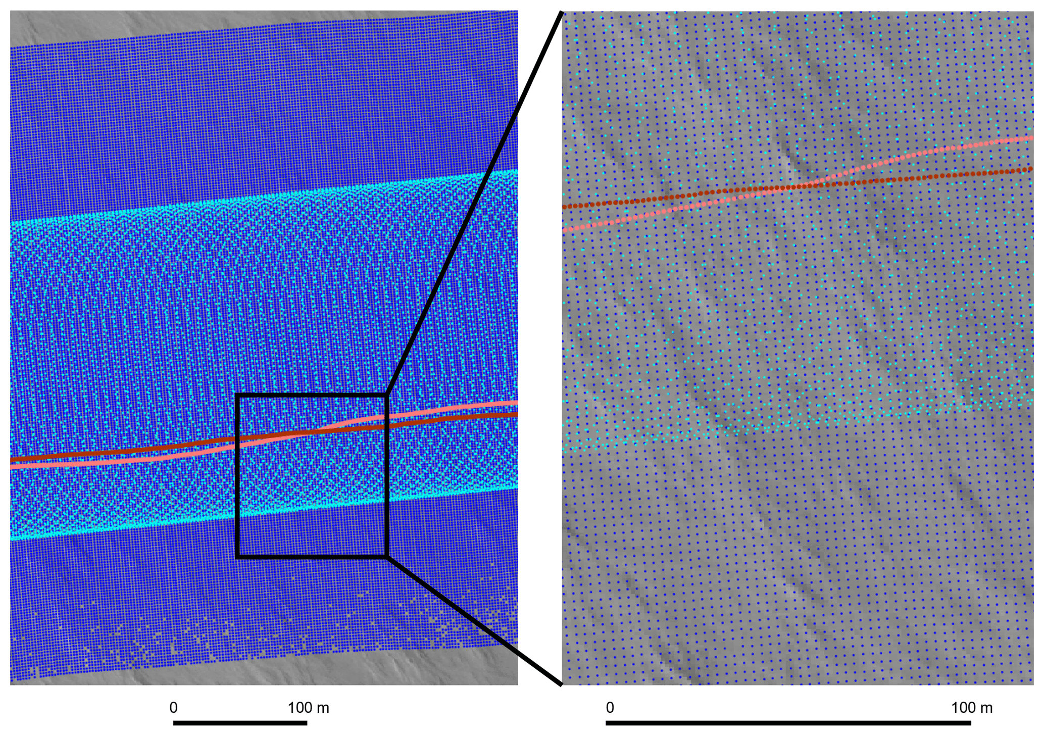
Figure 3 Sample footprint spacing for the UAF lidar (dark blue) and ATM (cyan), and the 88S Traverse ground-based GPS data are in shades of red (GPS A is in light red while GPS B is in dark red). WorldView-2 imagery, copyright 2017, DigitalGlobe, Inc.
2.2 UAF lidar
The University of Alaska Fairbanks (UAF) lidar is a line-scanner laser altimeter that has typically been deployed during Alaska-based OIB campaigns (Johnson et al., 2013). The UAF lidar surveyed the 88S Traverse on two separate flights (30 November and 3 December 2017) while integrated in a commercial (Airtec) BT-67 (Basler). The UAF system is a commercial RIEGL LMS-Q240i scanning laser altimeter transmitting in the 905 nm wavelength part of the spectrum. The system has a full scanning angle of 60∘. The two surveys over the 88S Traverse were conducted at an aircraft speed of ∼85 m s−1, at an altitude of ∼450 m a.g.l. (above ground level). At this speed and altitude, and with an effective repetition rate of 10 kHz, the UAF lidar generates a ∼1.3 m diameter footprint with a total across-track swath width of ∼500 m. Within a 10 m by 10 m area, the UAF lidar produces ∼20 to 25 returns, with nearly uniform footprint spacing of ∼2 m (Fig. 3).
2.3 Airborne Topographic Mapper (ATM)
ATM (Krabill et al., 2002; Martin et al., 2012) is a laser altimetry system used by many OIB campaigns in both the Arctic and Antarctic. ATM collected data along the 88S Traverse on 26 October 2014, while integrated on the NASA DC-8. For that deployment, ATM (version T4) consisted of a dual instrument configuration, with both wide-scan and narrow-scan lidar systems integrated simultaneously. The wide-scan lidar system is more appropriate for ice sheet surveys and has a full scanning angle of 30∘. The ATM lidars are full-waveform conically scanning systems, transmitting 532 nm wavelength 6 ns pulses. Surveys were conducted at an aircraft speed of ∼100 m s−1, at an altitude of ∼450 m a.g.l. At this speed and altitude, and with a 3 or 5 kHz repetition rate, the wide-scan (30∘) ATM lidar generates a ∼1 m diameter footprint with a scanning swath width of ∼250 m. Within a 10 m by 10 m area, the wide-scan ATM produces about six to eight returns, with a nonuniform footprint spacing of ∼5 m; data are most dense along the edge of the swath (Fig. 3).
For completeness, we note that ATM also conducted a mission that included the 88S Traverse on 26 October and 15 November 2016 (also integrated on the NASA DC-8 and flying at ∼450 m a.g.l.) using the T6 version of ATM. However, analysis of these data and other flights during this campaign suggest that there is an across-track tilt within these data, which represented a 10 to 15 cm spurious elevation variation across the wide-scan ATM swath (Michael Studinger, NASA, personal communication, 2018). We therefore exclude the 2016 ATM flights from further discussion.
3.1 88S Traverse GPS data
Following the data processing methods of Brunt et al. (2017), we post-processed 88S Traverse GPS data using PPP methods. PPP solutions use precise GPS satellite orbit and clock information to determine the kinematic GPS antenna position. Position solutions for each vehicle were determined using NovAtel's Inertial Explorer (v.8.6); processing for each vehicle was performed on nearly continuous stretches of GPS data, which typically represented 1 full day of driving, or approximately 50 km. Position solutions were solved to the L1 phase center of each antenna; the elevations are given in the ITRF08 reference frame and the geographic coordinates are referenced to the WGS84 ellipsoid. We used a GPS satellite elevation mask, or a cutoff angle, of 7.5∘ to minimize the effects of GPS multipath error. Inertial Explorer provides an estimate of a given point-position vertical accuracy; this value was used to filter suspect elevation data that had a vertical sigma of more than 8 cm.
The elevation of the snow surface, relative to the position solutions of the L1 phase center of each antenna (Fig. 2), was then determined using data from the field and the appropriate National Geodetic Survey (NGS) antenna model phase-center offset. The height of the snow surface (h) for each vehicle was determined based on the position solutions of the GPS antenna phase centers (GPSPC) based on the following equation:
where hAntHeight is the mean distance between the antenna base plane and the indentation of the tracks in the snow (281.3 or 282.3 cm, depending on the vehicle), hNGSmodel is the distance between the antenna phase center and the base plane based on the NGS model for the Trimble Zephyr 2 Geodetic antenna (4.1 cm), and hTrackDepth is the mean depth of the PistenBully track indentations into the snow surface (6.2 or 5.8 cm, depending on the vehicle).
3.2 Airborne lidar data
We obtained the UAF Lidar Scanner L1B Geolocated Surface Elevation Triplets, version 1 data (Larsen, 2010) through the National Snow and Ice Data Center (NSIDC) OIB Data Portal (http://nsidc.org/icebridge/portal/, last access: July 2018) for the 30 November and 3 December 2017 flights over the 88S Traverse area (files available at NSIDC are associated with whole Julian days, or days 334 and 337). The data files consist of latitudes, longitudes, and elevations that were derived from an integrated on-board GPS (Trimble) and inertial system (OxTS Inertial+2). GPS post-processing used PPP methods using NovAtel's GrafNav (v.8.4). Processing of the lidar data, including the incorporation of the GPS and inertial data used a commercial software package (RiProcess) developed by RIEGL. These data are distributed with the elevations given in the ITRF08 reference frame and the geographic coordinates referenced to the WGS84 ellipsoid.
We also obtained the ATM IceBridge ATM L1B Elevation and Return Strength with Waveforms, version 1 data (Studinger, 2018) through the NSIDC for the 26 October 2014 flight over the 88S Traverse area (17:04 to 19:45 UTC). The data files include geographic coordinates and elevations derived from an integrated on-board GPS (Javad) and inertial system (Applanix POS AV). Differential GPS (DGPS) post-processing methods use a base station installed at the departure airport for this deployment. DGPS was accomplished using a software package developed by the ATM team called GITAR (GPS Inferred Trajectories for Aircraft and Rockets; Martin, 1991). These data are distributed with the elevations given in the ITRF08 reference frame and the geographic coordinates referenced to the WGS84 ellipsoid.
3.3 Comparison strategy
We based our comparison strategy on Brunt et al. (2017). We compared the post-processed snow surface elevations from the 88S Traverse with the airborne surface elevation data, using a nearest-neighbor approach. In this method, we compared the closest lidar data point to every single ground-based GPS data point. We limited our statistical analysis based on a distance criterion, making elevation comparisons only where the lidar footprints and the GPS measurements were within a distance 1 m of one another. We then assessed the difference between the filtered GPS and ATM and UAF lidar surface elevation datasets.
Once the lidar elevation data (Lidarelevation) are associated with the GPS elevation data (GPSelevation), the mean elevation difference (GPSelevation – Lidarelevation) is the lidar elevation bias (B). We note that we take the GPS elevation data to be the ground truth.
The 1σ standard deviation of this airborne lidar elevation bias (B) is the spread of the lidar data, or the precision, about the mean. This is also the vertical dispersion of the lidar measurements about the mean surface. The vertical dispersion, or the surface measurement precision, includes both instrument precision and geophysical properties of the surface that will affect the measurement. Instrument precision is related to factors such as instrument timing errors, geolocation knowledge, and footprint size. Geophysical properties that will affect the measurement include atmospheric effects, surface roughness, and surface slope, although we note that our analysis is limited to a region of low (less than 1∘) surface slope. These instrument and geophysical effects cannot be uniquely distinguished within the surface measurement precision. Ultimately, we report elevation accuracies and surface measurement precisions as a residual, following the convention of mean bias ±1σ standard deviation, or 0.0±0.0 cm.
The lidar biases and precisions reported here are determined relative to the GPS data, which we take to represent truth, with zero errors. In actuality, these errors are not zero and are a function of (1) formal GPS errors, which include factors such as ephemeris and clock errors; (2) ionosphere and troposphere errors; (3) multipath errors; and (4) errors due to geophysical effects, such as variable snow surface strength causing variable vehicle sinking or antenna motion due to short-scale surface undulations (sastrugi). We note that given the short distance between the two survey vehicles, our results are somewhat blind to the full magnitude of the error terms that can be correlated on short timescales, such as those associated with the ionosphere and troposphere.
4.1 Ground-based GPS data evaluation
We compared the GPS position solutions of each vehicle to assess consistency of the ground-based data. After the 88S Traverse GPS data for each vehicle were post-processed, the data were then filtered based on the 8 cm vertical sigma; this reduced each GPS dataset by about a third (GPS unit A: 316 948 data points were reduced to 203 603; GPS unit B: 321 689 data points were reduced to 209 253). The mean vertical sigma values for the data used in further analysis were 7.16 and 7.19 cm for ground-based GPS units A and B, respectively. We then used a nearest-neighbor approach, limited based on a 0.5 m distance criterion, and calculated the mean elevation residual between the elevation measured by the two vehicles. This residual was 1.1±4.1 cm (n=26 442).
PPP GPS post-processing methods are often used in regions where long-term base-station data are not available for DGPS methods, such as the center of ice sheets. Brunt et al. (2017) showed that PPP position solutions for their traverse outside of Summit Station, in the center of the Greenland Ice Sheet, were comparable to GPS position solutions using differential methods. Therefore, while we are limited with respect to the availability of permanent GPS base stations for post processing, we feel confident that our methods provide consistent and accurate results and are appropriate for this data analysis.
4.2 Airborne lidar evaluation
To assess the internal consistency of the UAF lidar, we compared the processed elevation data from the 30 November 2017 flight to the 3 December 2017 flight, using a nearest-neighbor approach, limited based on a 1 m distance criteria, and calculated the mean elevation residual. This residual was 8.1±10.5 cm (n>1.5 million data points); data from the 30 November 2017 flight were lower than data from the 3 December 2017 flight. A similar assessment of internal consistency of the ATM data could not be made since our analysis was limited to a single flight, after rejecting the 2016 ATM data due to an observed across-track tilt.
4.3 GPS to airborne lidar results
Table 1 lists the results for the nearest-neighbor analysis of the ground-based GPS and lidar elevation comparisons for both ATM and the UAF lidar. Both altimeters had elevation biases of less than 10 cm and surface measurement precisions of less than 15 cm; we note that these values are similar to those in Brunt et al. (2017), which is a similar study in a similar geophysical setting. Figure 4a shows the elevations of ground-based GPS unit A. Panel (b) shows the difference between GPS A elevations and the 30 November UAF lidar elevations, minus the mean difference. Panel (c) is similar to panel (b) but using the 3 December UAF lidar data, and panel (d) compares the GPS data to the 2014 ATM data. Figure 5 is the same as Fig. 4, but the results are relative to ground-based GPS unit B.
Table 1Elevation bias and surface measurement precision (cm), relative to ground-based GPS survey data, for ATM and UAF airborne lidar elevation data. Results are posted as GPSelevation – Lidarelevation.
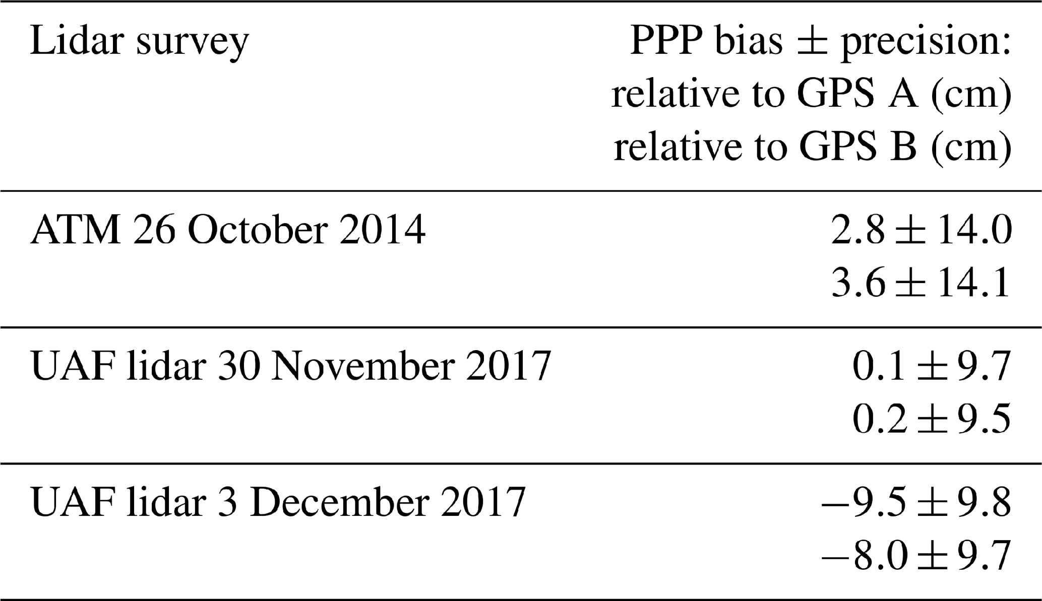
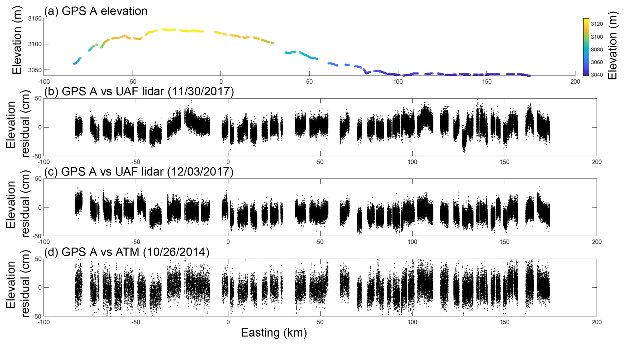
Figure 4Along-track elevation and elevation differences associated with GPS A. (a) Along-track elevation of GPS A, in meters. (b) Elevation difference between GPS A and the UAF lidar (30 November 2017), minus the mean difference. (c) Elevation difference between GPS A and the UAF lidar (3 December 2017), minus the mean difference. (d) Elevation difference between GPS A and ATM (26 October 2014), minus the mean difference.
We examined the spatial correlation of the elevation differences calculated between the ground-based GPS data and the airborne lidar data (Motyka et al., 2010; Rolstad et al., 2009). When measurements are made within close spatial proximity of one another, they are generally similar, and measurement errors tend to be correlated; over increasing distances, measurement errors become uncorrelated. Similar to Rolstad et al. (2009), which is a detailed summary of semivariograms, we created semivariograms of the elevation differences. This analysis is intended to provide an assessment of the length scales at which measurement errors become independent of one another, or uncorrelated. Figures 6 and 7 provide the semivariograms for GPS units A and B, respectively, relative to the two UAF lidar flights (Figs. 6a, b and 7a, b) and the ATM flight (Figs. 6c, 7c). The x axes are lag distances between the observations, in meters, and the y axes are the measure of variance, in square meters. The red squares represent the observed elevation differences in 50 m bins and the lines represent a semivariogram model fit to these data. The range and the sill of the variograms are interpreted to be where the slope of the model fit to the variance asymptotes toward zero, which is indicated where the lines in the figures change from blue to red. At this distance, or at the range value, the observations are considered to have become independent; from Figs. 6 and 7, we estimate that the range at which the variance starts to be relatively unchanging, and the length scale at which measurement errors become uncorrelated, is ∼10 to 50 m. These results are based on 5 km of along-track data; semivariograms based on longer length scales (20 km) had similar results. We attribute this 10 to 50 m length scale to be associated with wind-driven surface processes and overall roughness (sastrugi), as visible in the background of Fig. 3. Sastrugi cause noise about the mean surface elevation from a measurement perspective and we assume that this is the largest source of correlated error, given the size of the footprints of the observations (1 to 2 m), the distance criteria associated with the differencing methods (1 m), and the length scale of the surface roughness associated with sastrugi (5 to 10 m).
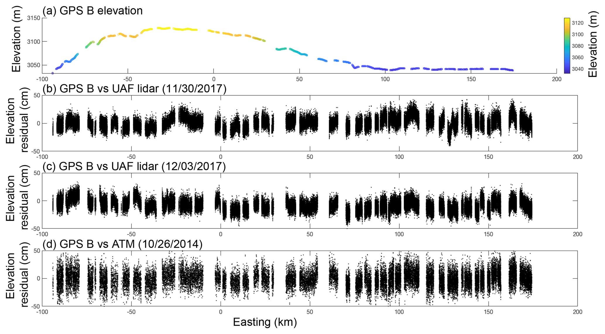
Figure 5Along-track elevation and elevation differences associated with GPS B. (a) Along-track elevation of GPS B, in meters. (b) Elevation difference between GPS B and the UAF lidar (30 November 2017), minus the mean difference. (c) Elevation difference between GPS B and the UAF lidar (3 December 2017), minus the mean difference. (d) Elevation difference between GPS B and ATM (26 October 2014), minus the mean difference.
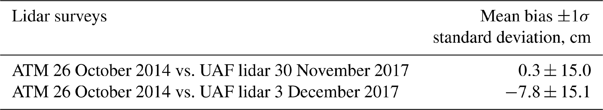
Table 2Elevation bias and surface measurement precision (cm), between ATM and the UAF lidar. Results are posted as ATMelevation – UAFelevation.
The 1σ mean elevation residual between the two GPS units for this study was 1.1±4.1 cm (n=26 442), with GPS A generally being higher than GPS B. This residual compares favorably to the GPS assessments of Brunt et al. (2017) and Kohler et al. (2013), the studies that most closely match the methods and geophysical setting presented here. Brunt et al. (2017) reported a 1σ mean elevation residual of 0.7±5.7 cm, based on comparisons between two different passes of the traverse occurring on the same day and using the same GPS unit (n=710). Kohler et al. (2013) reported a 1σ mean elevation residual of 0.6±7.5 cm, based on crossovers between two different GPS units during the traverses (n=1131). We attribute the quality of our GPS data to (1) the long length scale of data collection (relative to Brunt et al., 2017) and (2) the flat surface that defined our traverse route (relative to Kohler et al., 2013).
While the residual between the 88S Traverse vehicles is low, it is not zero. We attribute the ∼1 cm bias between our GPS datasets to uncertainties in the measurements of track depth. From Eq. (1) and Fig. 2, the three terms associated with reducing the GPS measurement to a snow-surface height are the phase center offset (which is static and common between the vehicles), the antenna height (vehicle A 281.3±0.9 cm; vehicle B: 282.3±0.4 cm), and the track depth (vehicle A: 6.2±1.6 cm; vehicle B: 5.8±1.2 cm). Given the uncertainties associated with the two field-based measurements (antenna height and track depth), we feel confident that the snow depth is the leading term in the height uncertainty. As stated above, we note that we are blind to errors introduced by the close spatial coincidence of the GPS receivers (∼50 m) and to those introduced by the common processing of the GPS data. Errors in ionospheric or tropospheric modeling would impact both GPS-based datasets similarly and would introduce a bias between the GPS measurements and the actual ice sheet surface.
Overall, the quality of the lidar data used in this survey was quite good. While a quantitative assessment could be made for the UAF lidar, a similar assessment of ATM could not be made in this region, as we were limited to one flight. However, Brunt et al. (2017) analyzed ATM data from five different airborne campaigns, which included five different versions of the ATM system (including both narrow and wide scanning data) near Summit Station, Greenland, on the relatively flat ice sheet interior, similar to this study. Their results indicated an average ATM elevation bias and surface measurement precision of cm (based on PPP post-processing, which is the method used here). These results match well with those of Martin et al. (2012), who summarize the vertical accuracy and precision of ATM over ice sheets to be 6.6±3 cm. Given that we are using the same lidar, with similar survey techniques, over a similar surface, we consider ATM to be a stable instrument, with data quality suitable for this application.
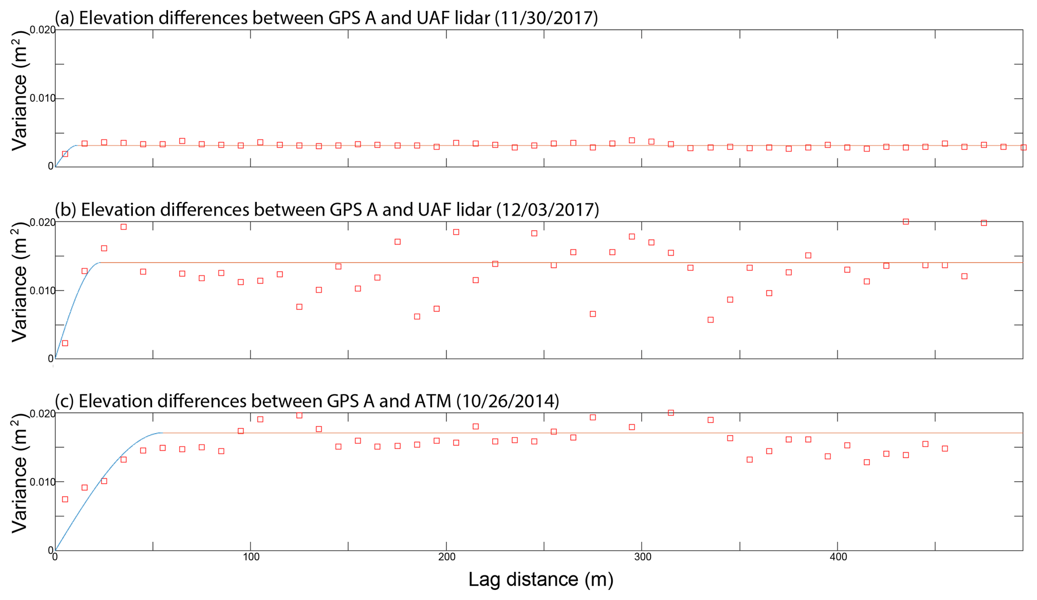
Figure 6Semivariograms of elevation differences between GPS unit A and elevations derived from ATM (a) and the UAF lidar on 30 November 2017 (b) and 3 December 2017 (c). The x axes are lag distances between the observations, in meters, and the y axes are variance, in square meters. The red squares are the observed elevation differences in 50 m bins and the lines represent a semivariogram model fit to these data.
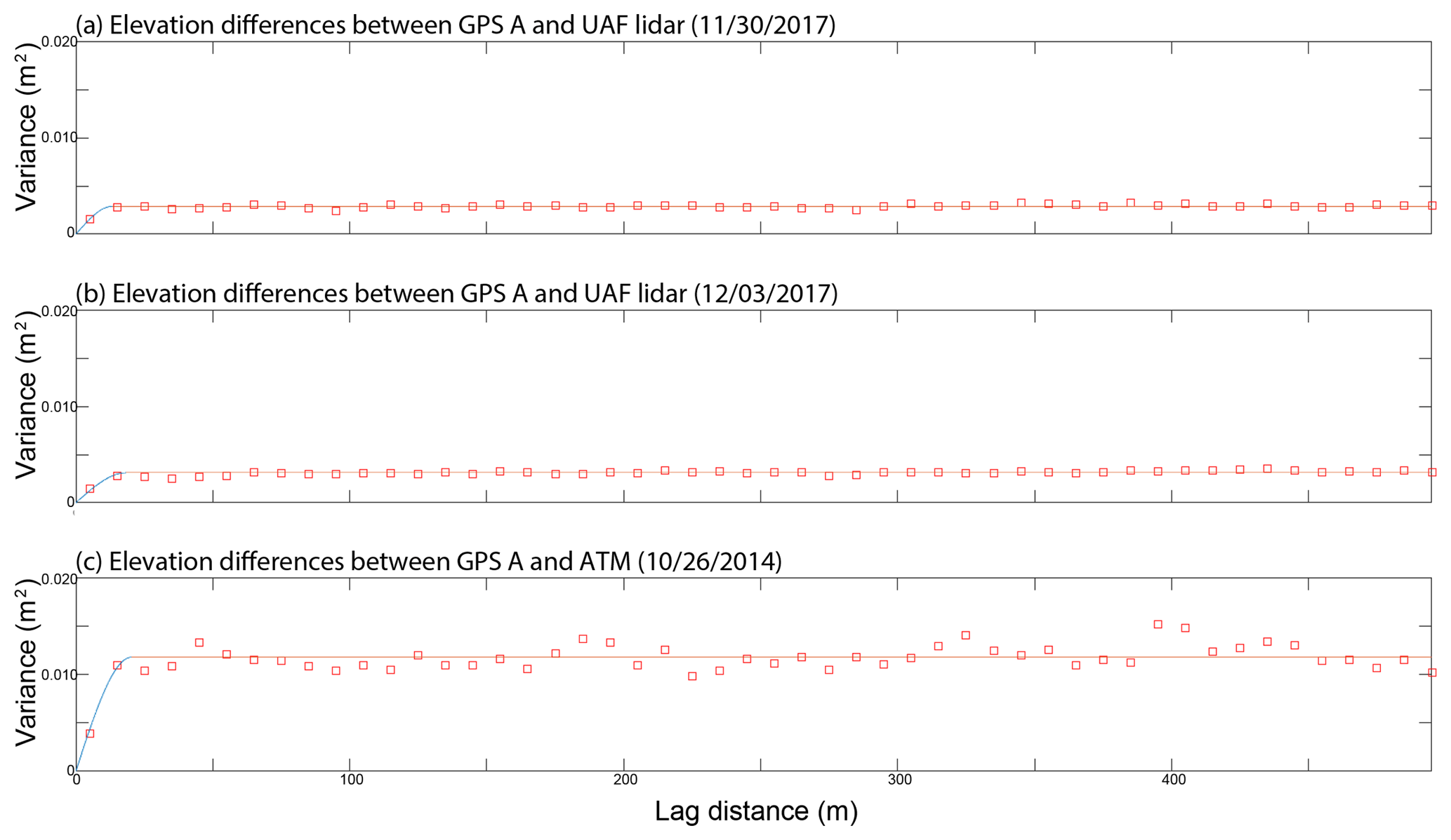
Figure 7Semivariograms of elevation differences between GPS unit B and elevations derived from ATM (a) and the UAF lidar on 30 November 2017 (b) and 3 December 2017 (c). The x axes are lag distances between the observations, in meters, and the y axes are variance, in square meters. The red squares are the observed elevation differences in 50 m bins and the lines represent a semivariogram model fit to these data.
We note that there is a slight along-flight signature that is apparent in the UAF lidar elevation data (Fig. 8). The signature is visible in the southern side of the swaths of both the 30 November and 3 December 2017 datasets. Specifically, there appears to be a trough along the southern edge of the swaths that has anomalously lower elevations, relative to the surrounding edges. The magnitude is variable but based on a nearest-neighbor assessment of the overlapping region in Fig. 8, where the flight line from 30 November 2017 intersected itself; the mean residual was cm. While the source of this artifact is still undetermined, it does not appear to be an across-track tilt. This effect on measured elevation is small (∼5 cm from edge of the trough to the base of the trough) and generally limited to near the edge of the lidar swath (Fig. 8). These data were typically not used for ground survey GPS comparison, as the ground-based data generally intersected the center of the swath, where we believe the data quality is not compromised.
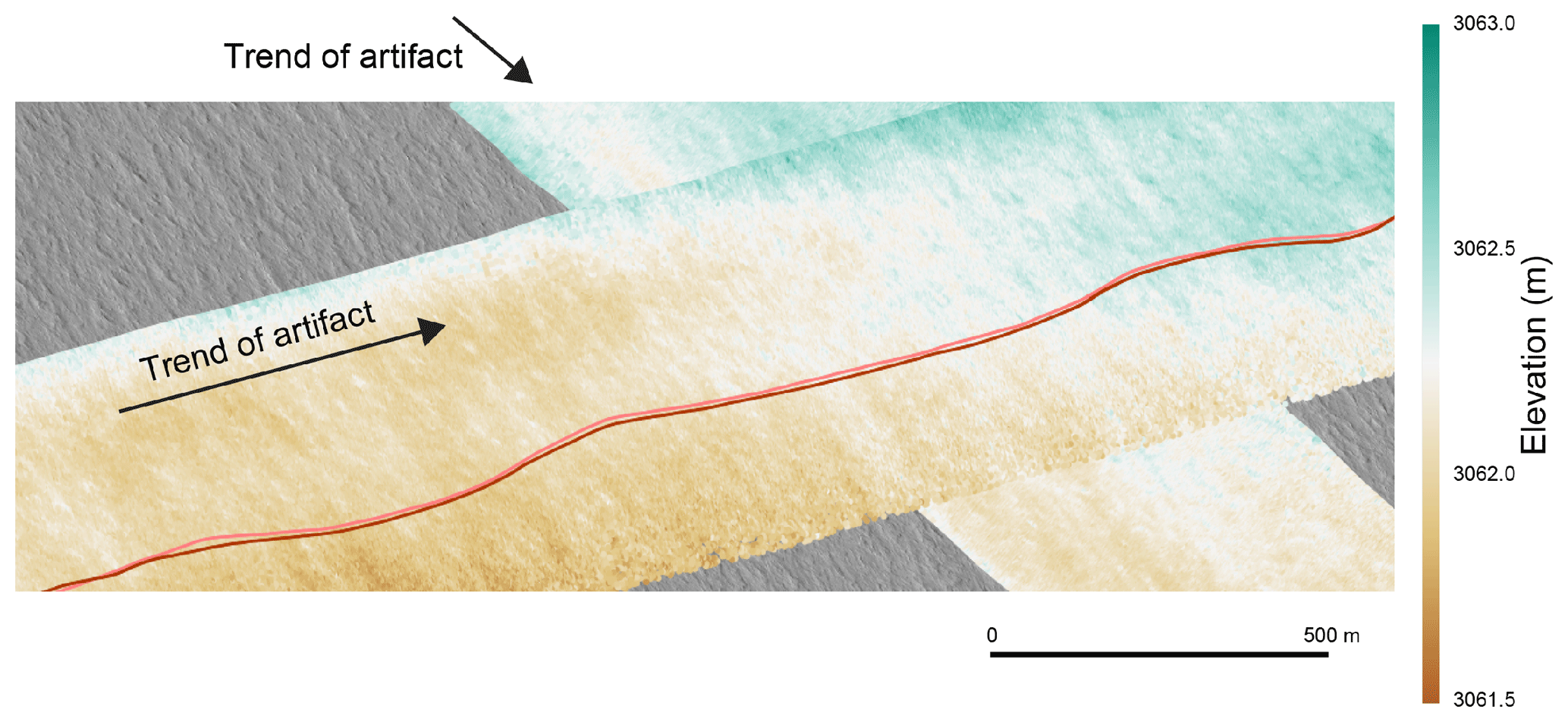
Figure 8Elevation data from the UAF lidar (30 November 2017), where the flight line crossed itself. The along-track artifact in the data is visible in both passes; UAF lidar elevations are anomalously lower within the artifact and manifest as a narrow trough, parallel to the direction of flight. 88S Traverse ground-based GPS data are in shades of red. WorldView-2 imagery, copyright 2017, DigitalGlobe, Inc.
The elevation biases and surface measurement precisions of the two OIB lidars presented here are comparable to those of the OIB lidars assessed in Brunt et al. (2017); results based on PPP methods for both studies indicated biases that are less than ∼11 cm and measurement precisions that are less than ∼15 cm (Table 1 in this document and Table 2 in Brunt et al., 2017). Brunt et al. (2017) also indicate an average ATM elevation bias and surface measurement precision of cm. From Table 1, the surface measurement precision associated with ATM over the 88S Traverse (±14 cm; “lower precision”) was poorer quality than the average precision of ATM over the Summit Station Traverse (±7 cm; “higher precision”) as determined by Brunt et al. (2017). These two assessments had a similar geophysical setting (i.e., ice sheet interior) and similar survey strategies (GPS collection and processing methods).
We attribute the poorer surface measurement precision to the time difference between the airborne ATM campaign (October 2014) and the ground-based GPS survey (December 2017 to January 2018). Specifically, we hypothesize that these differences were associated with the transient locations of sastrugi. To assess this hypothesis, we used the same nearest-neighbor approach, described in the methods section, to compare the 2014 ATM elevation data to the 2017 UAF lidar elevation data (Table 2). Ultimately, the difference between these two lidar datasets revealed a signature that was of a similar magnitude (meters) and trend (∼150∘ line of longitude) as the sastrugi, based on observations of the sub-meter-resolution WorldView-2 satellite imagery, obtained via the Polar Geospatial Center at the University of Minnesota (Fig. 9).
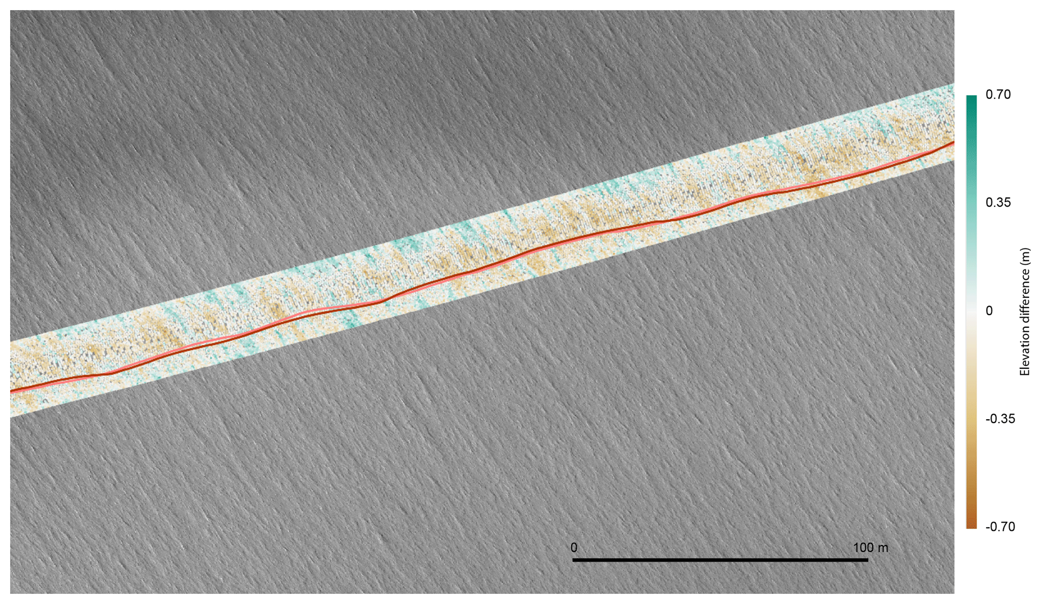
Figure 9Ground-based GPS data (in shades of red) plotted on difference in elevation between ATM (26 October 2014) and the UAF lidar (30 November 2017). WorldView-2 imagery, copyright 2017, DigitalGlobe, Inc.
Sastrugi cause noise about the mean surface elevation from a measurement perspective. Sastrugi migration between the 2014 ATM campaign and the 2017/2018 ground-based traverse would not have an impact on the surface elevation bias, as the observed differences would be averaged out and lost in surface measurement noise. The migration of the sastrugi adds components of noise on the mean surface measurement. This effect is evident in the observed larger (poorer) ATM surface measurement precision assessment.
We note that our analysis does not attempt to account for elevation changes due to the temperature- and accumulation-rate-driven effects of firn compaction (Li and Zwally, 2015). In this region, we expect variation in firn compaction rate to be driven by changes in firn temperature, which have a large seasonal amplitude and a much smaller secular trend. As the firn warms each austral spring, the surface elevation along our traverse should decrease. Since the UAF lidar data and ground-based GPS data were collected within a month, we expect firn compaction to have a negligible effect on our results. Conversely, the ∼2-month seasonal lag between the ATM and GPS data collection means that we may be sensitive to the seasonality of firn compaction rate, as well as any secular trend over the 4-year interval between these datasets.
Overall, these results suggest that the 88S Traverse route is an ideal setting to assess airborne or satellite absolute elevation accuracy (Brunt et al., 2017), as the surface was relatively unchanged between 2014 and 2018 (i.e., no distinguishable change in bias). Further, our results based on the 2014 ATM elevation dataset suggest that airborne data collected along this route are applicable to absolute elevation validation for a few years. However, results based on our comparisons between our GPS measurements and ATM suggest that when a few years have passed between the datasets being evaluated, the surface elevation measurements become hard to reproduce; this manifests itself in a higher surface measurement precision assessment.
Data collected from the 88S Traverse (and data collected on subsequent surveys of the same route) will provide 300 km of in situ data for direct comparison with ICESat-2 elevation data products. The GPS data collection strategies and post-processing methods presented here provide accurate and precise data for such an assessment. Further, the data analysis presented here provides guidance on how to make similar comparisons between ground-based and satellite elevations, given the satellite footprint size and associated rejection criteria. Approximately three to four ICESat-2 reference ground tracks will intersect this region daily to produce many statistical crossover points between the GPS and ICESat-2 datasets. While the crossover points represent only a small segment of along-track ICESat-2 data, the analysis will be based on data from many ICESat-2 reference ground tracks over the course of the entire satellite mission. Thus, the analysis of the derived ICESat-2 bias and surface measurement precision relative to these GPS data will provide an assessment ICESat-2 performance through time, independent of errors associated with single orbits or single points in time. Results of Brunt et al. (2017) and results presented here also provide an assessment of the accuracy and surface measurement precision of three airborne lidars that NASA has routinely deployed over the ice sheets (ATM, LVIS, and the UAF lidar). With a statistical understanding of how these instruments perform on the relatively flat ice sheet interiors, longer flight lines can be constructed over similarly flat ice sheet surfaces to create better statistics associated with comparisons using long length scales of along-track ICESat-2 data. In summary, the strategic location of the ground-based 88S Traverse provides a validation of ICESat-2 that is independent of the errors that are correlated with respect to most satellite timescales, and these ground-based data provide a better understanding of airborne lidars that will survey longer length scales of data, for better satellite error statistics.
Here we present a comparison of in situ GPS elevation data and laser altimetry in preparation for ground-based and airborne validation of ICESat-2. We show that the ground-based methods for GPS data collection and processing along the 88S Traverse provide internally consistent results, with accuracies and precisions appropriate for assessing airborne lidar data and ultimately satellite elevation data. Further, we have shown that airborne lidar data assessed here (ATM and the UAF lidar), relative to the GPS data, show elevation biases that are comparable to results from similar instruments in similar geophysical settings. However, discrepancies between the ATM surface measurement precisions observed here, and those observed in Brunt et al. (2017) under similar ice sheet interior conditions, suggest that the migration of sastrugi can have an adverse effect on assessments of surface measurement precision when significant time (on the order of a few years) has elapsed between surveys. Thus, absolute elevation bias can be determined with datasets from this surface that are a few seasons old, but for the best assessment of precision, comparisons need to be made with relatively coincident (spatial and temporal) datasets.
The ground-based GPS data associated with this study are available online, as the Supplement related to this article. NASA ATM and the UAF lidar data are publicly available on the NSIDC Operation IceBridge Data Portal (http://nsidc.org/icebridge/portal/, last access: July 2018). WorldView-2 imagery is available to NSF- and NASA-funded researchers via the Polar Geospatial Center at the University of Minnesota.
The supplement related to this article is available online at: https://doi.org/10.5194/tc-13-579-2019-supplement.
KMB conducted the traverse, processed the ground-based GPS data, and led the effort to make the comparisons between these data and the airborne lidar data. TAN conducted the traverse and was instrumental in the effort to make the comparisons with the airborne lidar. CFL conducted the UAF lidar campaign and processed those data. All authors contributed to the discussion of the results and shared the responsibility of writing this paper.
The authors declare that they have no conflict of interest.
We thank the NASA ICESat-2 Project Science Office for funding the field
component and data analysis associated with this project. We thank the
National Science Foundation, Office of Polar Programs for logistical support
of the field component of this project. We thank Operation IceBridge for the
data collection of the ATM and UAF lidar datasets. We thank our deep-field
mechanic and mountaineer associated with the 88S Traverse (Chad Seay and
Forrest McCarthy) for ensuring that we safely completed the full Antarctic
ground survey. We thank the many science support staff of the US Antarctic
Program that helped make the field component of this project possible. We
thank the National Snow and Ice Data Center (NSIDC) for IceBridge data
distribution. Finally, we thank our editor (Kenny Matsuoka) and the two
anonymous reviewers for constructive comments on earlier drafts of this
paper. WorldView-2 imagery was provided by the Polar Geospatial Center
at the University of Minnesota, which is supported by grant ANT-1043681 from
the National Science Foundation.
Edited by: Kenichi Matsuoka
Reviewed by: two anonymous referees
Bindschadler, R., Vornberger, P., Fleming, A., Fox, A., Mullins, J., Binnie, D., Paulsen, S., Granneman, B., and Gorodetzky, D.: The Landsat image mosaic of Antarctica, Remote Sens. Environ., 112, 4214–4226, https://doi.org/10.1016/j.rse.2008.07.006, 2008.
Brunt, K. M., Hawley, R. L., Lutz, E. R., Studinger, M., Sonntag, J. G., Hofton, M. A., Andrews, L. C., and Neumann, T. A.: Assessment of NASA airborne laser altimetry data using ground-based GPS data near Summit Station, Greenland, The Cryosphere, 11, 681–692, https://doi.org/10.5194/tc-11-681-2017, 2017.
Fricker, H., Borsa, A., Minster, B., Carabajal, C., Quinn, K., and Bills, B.: Assessment of ICESat performance at the salar de Uyuni, Bolivia, Geophys. Res. Lett., 32, L21S06, https://doi.org/10.1029/2005GL023423, 2005.
Johnson, A., Larsen, C., Murphy, N., Arendt, A., and Zirnheld, S.: Mass balance in the Glacier Bay area of Alaska, USA, and British Columbia, Canada, 1995–2011, using airborne laser altimetry, J. Glaciol., 59, 632–648, https://doi.org/10.3189/2013JoG12J101, 2013.
Koenig, L., Martin, S., Studinger, M., and Sonntag, J.: Polar airborne observations fill gap in satellite data, Eos T. Am. Geophys. Un., 91, 333–334, https://doi.org/10.1029/2010EO380002, 2010.
Kohler, J., Neumann, T., Robbins, J., Tronstad, S., and Melland, G.: ICESat elevations in Antarctica along the 2007–09 Norway–USA traverse: Validation with ground-based GPS, IEEE T. Geosci. Remote, 51, 1578–1587, https://doi.org/10.1109/TGRS.2012.2207963, 2013.
Krabill, W., Abdalati, W., Frederick, E., Manizade, S., Martin, C., Sonntag, J., Swift, R., Thomas, R., and Yungel, J.: Aircraft laser altimetry measurement of elevation changes of the Greenland ice sheet: Technique and accuracy assessment, J. Geodyn., 34, 357–376, https://doi.org/10.1016/S0264-3707(02)00040-6, 2002.
Larsen, C.: IceBridge UAF Lidar Scanner L1B Geolocated Surface Elevation Triplets, NASA NSIDC DAAC, Boulder, Colorado, https://doi.org/10.5067/AATE4JJ91EHC, 2010.
Li, J. and Zwally, H. J.: Response times of ice-sheet surface heights to changes in the rate of Antarctic firn compaction caused by accumulation and temperature variations, J. Glaciol., 61, 1037–1047, https://doi.org/10.3189/2015JoG14J182P, 2015.
Markus, T., Neumann, T., Martino, A., Abdalati, W., Brunt, K., Csatho, B., Farrell, S., Fricker, H., Gardner, A., Harding, D., Jasinski, M., Kwok, R., Magruder, L., Lubin, D., Luthcke, S., Morison, J., Nelson, R., Neuenschwander, A., Palm, S., Popescu, S., Shum, C., Schutz, R., Smith, B., Yang, Y., and Zwally, H.: The Ice, Cloud, and land Elevation Satellite-2 (ICESat-2): Science requirements, concept, and implementation, Remote Sens. Environ., 190, 260–273, https://doi.org/10.1016/j.rse.2016.12.029, 2017.
Martin, C.: GITAR Program Documentation, NASA contract #NAS5-31558 program document, Goddard Space Flight Center, Wallops Flight Facility, Wallops Island, VA, 1991.
Martin, C., Krabill, W., Manizade, S., and Russell, R.: Airborne Topographic Mapper Calibration Procedures and Accuracy Assessment, NASA Technical Memorandum 2012-215891, 2012.
Motyka, R., Fahnestock, M., and Truffer, M.: Volume change of Jakobshavn Isbræ, West Greenland: 1985–1997–2007, J. Glaciol., 56, 635–646, https://doi.org/10.3189/002214310793146304, 2010.
Rolstad, C., Haug, T., and Denby, B.: Spatially integrated geodetic glacier mass balance and its uncertainty based on geostatistical analysis: Application to the western Svartisen ice cap, Norway, J. Glaciol., 55, 666–680, https://doi.org/10.3189/002214309789470950, 2009.
Siegfried, M., Hawley, R., and Burkhart, J.: High-resolution ground-based GPS measurements show intercampaign bias in ICESat elevation data near Summit, Greenland, IEEE T. Geosci. Remote, 49, 3393–3400, https://doi.org/10.1109/TGRS.2011.2127483, 2011.
Studinger, M.: IceBridge ATM L1B Elevation and Return Strength with Waveforms, Version 1. NASA NSIDC DAAC, Boulder, Colorado USA, https://doi.org/10.5067/EZQ5U3R3XWBS, 2018.
Webb, C., Zwally, H., and Abdalati, W.: The Ice, Cloud, and land Elevation Satellite (ICESat) Summary Mission Timeline and Performance Relative to Pre-Launch Mission Success Criteria, NASA Technical Report, NASA/TM-2013-217512, 2012.
Zwally, H., Li, J., Brenner, A., Beckley, M., Cornejo, H., DiMarzio, J., Giovinetto, M., Neumann, T., Robbins, J., Saba, J., Yi, D., and Wang, W.: Greenland ice sheet mass balance: distribution of increased mass loss with climate warming; 2003–07 versus 1992–2002, J. Glaciol., 57, 88–102, https://doi.org/10.3189/002214311795306682, 2011.