the Creative Commons Attribution 4.0 License.
the Creative Commons Attribution 4.0 License.
 | 14 Feb 2019
On the timescales and length scales of the Arctic sea ice thickness anomalies: a study based on 14 reanalyses
Leandro Ponsoni
François Massonnet
Thierry Fichefet
Matthieu Chevallier
David Docquier
The ocean–sea ice reanalyses are one of the main sources of Arctic sea ice thickness data both in terms of spatial and temporal resolution, since observations are still sparse in time and space. In this work, we first aim at comparing how the sea ice thickness from an ensemble of 14 reanalyses compares with different sources of observations, such as moored upward-looking sonars, submarines, airbornes, satellites, and ice boreholes. Second, based on the same reanalyses, we intend to characterize the timescales (persistence) and length scales of sea ice thickness anomalies. We investigate whether data assimilation of sea ice concentration by the reanalyses impacts the realism of sea ice thickness as well as its respective timescales and length scales. The results suggest that reanalyses with sea ice data assimilation do not necessarily perform better in terms of sea ice thickness compared with the reanalyses which do not assimilate sea ice concentration. However, data assimilation has a clear impact on the timescales and length scales: reanalyses built with sea ice data assimilation present shorter timescales and length scales. The mean timescales and length scales for reanalyses with data assimilation vary from 2.5 to 5.0 months and 337.0 to 732.5 km, respectively, while reanalyses with no data assimilation are characterized by values from 4.9 to 7.8 months and 846.7 to 935.7 km, respectively.
- Article
(6047 KB) - Full-text XML
- BibTeX
- EndNote


The variability of the Arctic sea ice has received increasing attention from the scientific community over the past years (e.g., Chevallier and Salas-Mélia, 2012; Stroeve et al., 2014; Blanchard-Wrigglesworth and Bitz, 2014; Guemas et al., 2016). The main reason lies in the fact that Arctic sea ice plays a key role in the Earth's climate system (Budyko, 1969; Manabe and Stouffer, 1980b; Maykut, 1982). Among other contributions, it has been suggested that a decline of the Arctic sea ice extent and volume leads to a weakening of the Atlantic Meridional Overturning Circulation (Sévellec et al., 2017) and, therefore, potentially impacts the global distribution of heat (Drijfhout, 2015; Hansen et al., 2016). At the same time, the Arctic is one of the most sensitive regions to climate changes due to a phenomenon known as Arctic amplification (Manabe and Stouffer, 1980a; Holland and Bitz, 2003; Serreze et al., 2009). For instance, the current observed warming in the Arctic is reported to be nearly twice as large as other regions of the globe (Anisimov et al., 2007).
Other multiple specific interests from different stakeholders have reinforced the importance of sea ice projections, both at regional and larger scales, which include shorter shipping lanes (Lindstad et al., 2016), travel and tourism industry (Handorf, 2011), hunting and fishing activities (Nuttall et al., 2005), mineral resource extraction (Gleick, 1989), potential impact on the weather at midlatitudes (Walsh, 2014), environmental hazards (Nelson et al., 2002), and loss of weather predictive power by indigenous communities (Krupnik and Jolly, 2002). In this context, the sea ice thickness (SIT) is likely the most relevant state variable for monitoring, forecasting, and understanding recent and future changes of Arctic sea ice, first, because this parameter provides predictive information for the sea ice extent anomalies (Lindsay et al., 2008; Holland et al., 2011) and, second, due to the fact that SIT anomalies persist longer than sea ice extent anomalies, the former being reported as a forcing of the latter (Blanchard-Wrigglesworth et al., 2011).
However, direct observations of SIT and/or related parameters, namely draft and freeboard, are still sparse in time and space, despite the continuous efforts for compiling former and recent datasets from a range of sources (Lindsay, 2010; Lindsay and Schweiger, 2015). Some recent observational programs, such as the Year Of Polar Prediction (YOPP) (Jung et al., 2016) and the MOSAiC International Arctic Drift Expedition (https://www.mosaicobservatory.org/; last access: 15 July 2018), aim to enhance the Arctic observational system, being especially useful for improving our future modeling and forecasting skills.
Due to this lack of direct measurements in the past and present day, the ocean–ice reanalyses deserve special attention. A reanalysis product consists of models' outputs, which are generated over a certain time span by the same model, configurations, and procedures, and so are distributed onto regular grids, evenly stepped in time. These products are often built with assimilation of observational dataset(s) in order to improve the estimate of a certain parameter. For instance, SIT is often estimated by assimilating atmospheric, oceanic and, eventually, sea ice concentration data. The ocean–ice reanalyses are likely the main and more robust source of SIT data in terms of spatiotemporal resolution, being also broadly used for initialization and assimilation in other climate models (e.g., Guemas et al., 2016). Additionally, long-term reanalyses are crucial for understanding the past Arctic sea ice characteristics, in a period when in situ observations of ice parameters were inexistent.
In this work we make use of 14 state-of-the-art reanalyses in order to study two important aspects of the SIT predictability: the timescale (or persistence) and the length scale of SIT anomalies (see Sect. 2.3). Their importance is reinforced by the fact that the predictability of the SIT field depends on how long the anomalies persist over time and on how these anomalies spread in space. Notice that, hereafter, besides the traditional definition of time predictability, we adopt this term also for the spatial scale. In addition, timescales and length scales may also be useful for designing an optimal observation system when selecting ideal locations for deploying instruments as well as for defining a frequency sampling strategy (Blanchard-Wrigglesworth and Bitz, 2014).
Blanchard-Wrigglesworth and Bitz (2014) reported SIT anomalies with typical timescales and length scales of about 6–20 months and 500–1000 km, respectively. These results reinforce the fact that the SIT anomaly persists longer compared to the sea ice area anomaly, which is reported with a timescale of 2–5 months (Blanchard-Wrigglesworth et al., 2011; Day et al., 2014). Blanchard-Wrigglesworth and Bitz (2014) suggested that the SIT anomalies from models characterized by a thinner mean ice state tend to present shorter persistence but larger spatial scales. Blanchard-Wrigglesworth et al. (2011) reported a decline in the timescale of sea ice volume anomalies, as a result of the ice thinning induced by recent climate changes.
The first aim of this study is to evaluate the performance of different reanalysis products regarding their SIT realism by comparing these reanalyses against observational datasets. A point of main interest is to identify whether or not the assimilation of sea ice concentration by the reanalyses improves the representation of SIT. Second, we seek to characterize the timescales and length scales of the Arctic SIT anomalies. Again, we verify whether or not sea ice data assimilation plays a role in the temporal and spatial scales of SIT anomalies. Furthermore, we investigate the long-term evolution of timescales and length scales, as well as the relationship between these two parameters.
The paper is organized as follows: Sect. 2 introduces the reanalysis products, the observational datasets, and the respective methods applied in this research; Sect. 3 compiles all results, including the comparison between observations and reanalyses (Sect. 3.1), the comparison of reanalyses themselves (Sect. 3.2), and the patterns of timescales (Sect. 3.3) and length (Sect. 3.4) scales. Lastly, Sect. 4 draws discussion and conclusions on the findings reported in the previous sections.
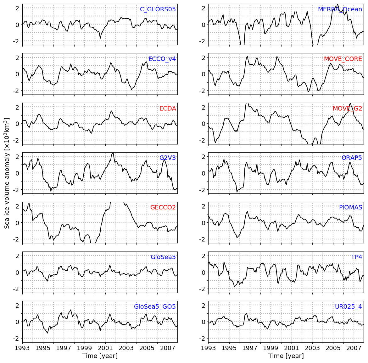
Figure 1Sea ice volume anomalies estimated from all reanalyses. Anomalies are calculated by excluding the trend and the seasonal cycle. Tick labels are placed at the first day of the respective year. Reanalyses labeled in blue and red highlight whether the datasets were built with or without sea ice data assimilation, respectively.
2.1 Sea ice reanalyses
Monthly fields of SIT from 14 state-of-the-art ocean–ice reanalyses are used in this work. All but one were compiled in the context of the ORA-IP project (Balmaseda et al., 2015; Chevallier et al., 2017; Uotila et al., 2018). The ORA-IP reanalyses (and their respective author/provider institution) are C-GLORS05 (CMCC; Storto et al., 2014), ECCO-v4 (JPL/NASA, MIT, AER; Forget et al., 2015), ECDA (GFDL/NOAA; Zhang et al., 2013; Chang et al., 2013), G2V3 (Mercartor Océan; Ferry et al., 2010), GECCO2 (University of Hamburg; Köhl, 2015), GloSea5 (UK Met Office; Blockley et al., 2014), GloSea5-GO5 (UK Met Office; Megann et al., 2014), MERRA-Ocean (GSFC/NASA/GMAO; Rienecker et al., 2011), MOVE-CORE (MRI/JMA; Danabasoglu et al., 2014), MOVE-G2 (MRI/JMA; Toyoda et al., 2013), ORAP5 (ECMWF; Zuo et al., 2015; Tietsche et al., 2017), TOPAZ4 (ARC MFC; Sakov et al., 2012; Xie et al., 2017) and UR025-4 (University of Reading; Valdivieso et al., 2014). The 14th reanalysis is the Pan-Arctic Ice-Ocean Modeling and Assimilation System, PIOMAS (Zhang and Rothrock, 2003). For the abbreviations, the reader is referred to Appendix A. The original horizontal grids present different resolutions (Table 1), but for comparison, all reanalyses are interpolated onto a common grid of spatial resolution following Chevallier et al. (2017).
Specific characteristics of each reanalysis regarding horizontal resolution, ocean–sea ice model, atmospheric forcing data, subgrid-scale ice thickness distribution, ice dynamics (VP, viscous–plastic, or EVP, elastic–viscous–plastic), parameters for the ice strength formulation, air–ice drag coefficient, ocean–ice drag coefficient, and the presence (and respective method) of ice data assimilation are summarized in Table 1. For additional information the reader is referred to Chevallier et al. (2017) and/or to the respective providers.
Table 1Ensemble of reanalyses, their respective configurations and set of selected parameters.
P* and Cf are parameters for the ice strength formulations following respectively Hibler (1979) and Rothrock (1975).
2.2 Observational references
We use a compilation of 16 observational datasets available in the Unified Sea Ice Thickness Climate Data Record (Sea Ice CDR; Lindsay, 2010; http://psc.apl.uw.edu/sea_ice_cdr; last access: 15 July 2018). The Sea Ice CDR is a concerted effort to bring together a range of datasets in a consistent format but is originally sampled by different methods and spatiotemporal scales as well as being stored in a variety of formats. We use the post-processed version of the Sea Ice CDR data, which is distributed by monthly mean for moored upward-looking sonar (ULS) point measurements or 50 km averages for submarine, airborne, and satellite observations. If applicable, the Sea Ice CDR already provides the files corrected for data biases (e.g., Rothrock and Wensnahan, 2007b).
From these 16 datasets, 11 provide draft measurements, while the remaining 5 provide sea ice thickness data. Seven draft datasets were sampled by means of moored ULSs, namely North Pole Environmental Observatory (NPEO; Drucker et al., 2003; Rothrock and Wensnahan, 2007b), Beaufort Gyre Exploration Project (BGEP), Institute of Ocean Science (IOS) – Eastern Beaufort Sea (IOS-EBS) and – Chuck Sea (IOS-CHK), Alfred Wegener Institute – Greenland Sea (AWI-GS; Harms et al., 2001), Bedford Institute of Oceanography Lancaster Sound (BIO-LS; Pettipas et al., 2008; Prinsenberg and Pettipas, 2008; Prinsenberg et al., 2009), and Polar Science Center – Davis Strait (Davis_St; Drucker et al., 2003). Four other draft datasets are also based on ULS measurements but are installed on US and UK submarines: US Navy Submarines – Analog (US-Subs-AN), US Navy Submarines – Digital (US-Subs-DG; Tucker III et al., 2001; Wensnahan and Rothrock, 2005; Rothrock and Wensnahan, 2007b), UK Navy Submarines – Analog (UK-Subs-AN), and UK Navy Submarines – Digital (UK-Subs-DG; Wadhams and Horne, 1980; Wadhams, 1984).
From the ensemble of sea ice thickness datasets, the Ice Thickness Program run by Environmental Canada (CanCoast) is the only dataset providing direct measurement of ice thickness by means of ice boreholes. The NASA Operation IceBridge datasets (IceBridge-V2 and IceBridge-QL; Kurtz et al., 2013) are derived from an aircraft-mounted laser altimeter. Finally, two datasets come from satellite campaigns: the laser-altimeter-derived ICESat Mission-Goddard (ICESat1-G; Zwally et al., 2008) from National Aeronautics and Space Administration (NASA) and the radar-altimeter-derived CryoSat satellite data (CryoSat-AWI; Ricker et al., 2014) from the European Space Agency (ESA).
2.3 Methods
Reanalyses are compared against observations by selecting SIT values from the nearest grid points to the respective observational sites, during the same respective months. Complementary metrics are employed to evaluate the relationship between observations and reanalyses. When directly comparing SIT from reanalyses and observations, we estimate the root mean square error (RMSE), the correlation coefficient (R), and the mean residual sum of squares (MRSS) from the linear fit between both datasets, by having the reanalysis values as predictors and the observational values as predicted variables. Since SIT and draft are different variables, here we evaluate the strength of the linear relationship between them. Thus, when comparing SIT from reanalyses against draft from observations, we only estimate R and MRSS. In this work we do not account for snow variation in order to avoid adding uncertainties to the SIT fields.
SIT anomalies are derived by eliminating the trend and the seasonal cycle present in the time series. To do so, the trend is estimated separately for every month by means of a second-order polynomial fit and subtracted from the respective month. A second-order fit seems to better reproduce the trends when compared to the linear fit, although the results are very similar (not shown). The same method is applied for the analyses conducted with the pan-Arctic sea ice volume anomaly, derived from the SIT data, as illustrated in Fig. 1.
Grid point comparisons of SIT anomalies among all reanalyses are performed by means of RMSE and R maps, calculated over an overlapping period of 15 years, from January 1993 to December 2007. This time span corresponds to the period during which data are available from all reanalyses. Furthermore, as adopted by Blanchard-Wrigglesworth and Bitz (2014), only grid points wherein the mean ice thickness at the time of summer minimum is greater than 0.1 m are taken into account. This condition is valid for all reanalysis-based results, unless otherwise stated.
The timescale (or persistence) is derived from individual time series by calculating the lagged autocorrelation stepped forward by one measurement, equivalent to 1 month. The e-folding reference is used so that the persistence is assumed to be the time when the lagged autocorrelation curve crosses the 1∕e (∼0.3679) value, as proposed in previous works (e.g., Blanchard-Wrigglesworth and Bitz, 2014; Guemas et al., 2016). As an example, Fig. 2 displays the timescale derived from the mooring-based draft anomaly sampled in the framework of the BGEP at 150∘ W, 75∘ N, from August 2003 to August 2013 (Krishfield et al., 2013). Figure 2 also shows the timescales from the allocated reanalysis-based SIT anomalies. For this geographical location and time span, the draft anomaly from BGEP persists for about 3.7 months, while the SIT anomalies from the different reanalyses persist from 2.4 to 8 months. The persistence is estimated both from a regional and pan-Arctic perspective. First, it is calculated at each grid point, for all SIT anomaly time series. Second, it is estimated for the long-term (GECCO2 and MOVE-CORE) pan-Arctic ice volume anomalies. For the latter case, we evaluate how stable the e-folding timescale is over time by applying a moving (stepped by 1 month) and length-variable window (from 5 to 59 years). Here, we also investigate whether the moving timescale is marked by significant band(s) of variability. To do so, we applied wavelet analysis as proposed by Torrence and Compo (1998).
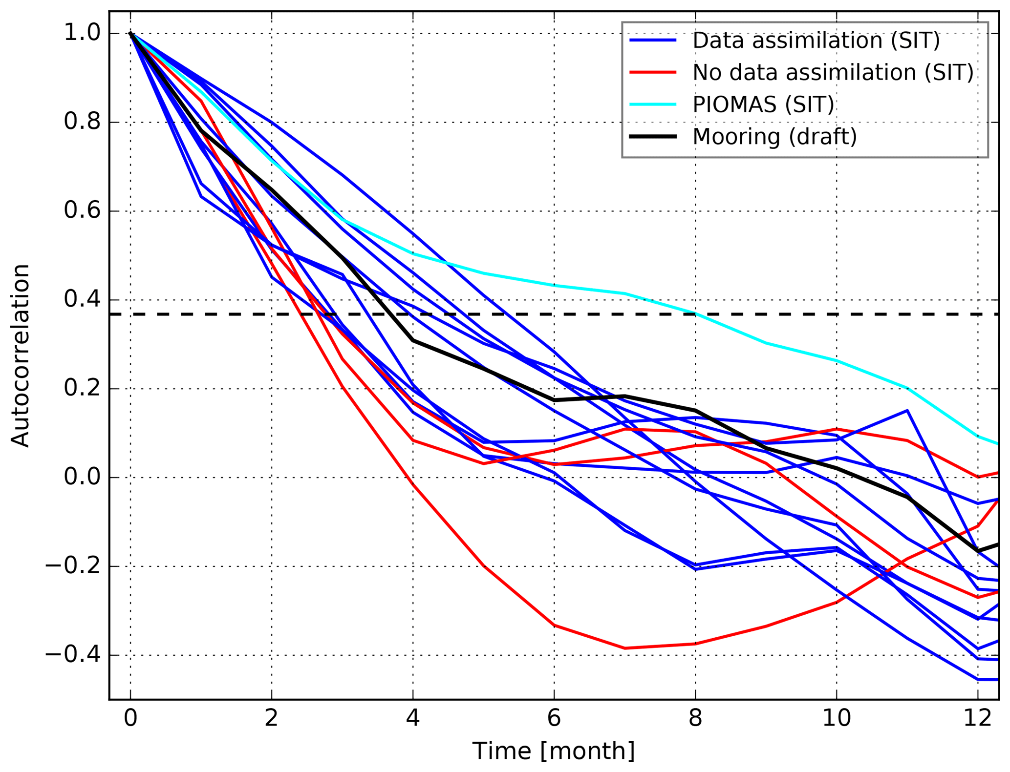
Figure 2Autocorrelation curves for the draft time series sampled in situ by upward-looking sonars deployed in the BGEP oceanographic mooring (black line). This mooring was placed at 150∘ W, 75∘ N (see location in Fig. 3c), and the data span from August 2003 to August 2013. The blue and red lines display the autocorrelation estimated from the SIT anomalies time series for the ORA-IP reanalyses, at the nearest grid point to the mooring and same time span, for the reanalyses built with and without sea ice data assimilation, respectively. The cyan line indicates the autocorrelation estimated for the PIOMAS reanalysis. The time in which the curves cross the black dashed line is defined as their respective e-folding timescales.

Figure 3(a) The e-folding length scale estimated from the CryoSat seasonal data of sea ice thickness. This dataset contains 14 spring (March–April) and autumn (October–November) fields, starting in autumn 2010 and finishing in spring 2017. (b) Same as (a), but using the equivalent temporal averages from the PIOMAS data. The difference between the fields shown in (a) and (b) is plotted in (c). The black circle in (c) indicates the location of the mooring from which data are used in Fig. 2.
The length scales of the SIT anomalies are estimated for the reanalysis datasets. The first step is to determine one-point correlation maps. In other words, we calculate the cross-correlation between the SIT anomaly from each grid point with the anomaly from all other points. Subsequently, we make use of the e-folding reference and, for every map, we select all grid cells with a correlation coefficient higher than 1∕e. The radius of a circle that yields the area covered by these selected cells is defined as the length scale of the SIT anomaly. This methodology is detailed and graphically presented by Blanchard-Wrigglesworth and Bitz (2014). Figure 3a shows an example for which the length scale is calculated for the SIT anomalies from CryoSat seasonal data: spring (March–April) and autumn (October–November), from autumn 2010 to spring 2017. In turn, Fig. 3b–c reveal that a similar length scale pattern is also present in PIOMAS. It is worth mentioning that this illustrative example allows a first assessment of how length scales from observations and reanalyses compare to each other. However, it can not be compared to the spatial scales of monthly anomalies further studied in Sect. 3.4.
3.1 Comparison of reanalyses with observations
The scatter plots shown in Fig. 4 combine SIT from each reanalysis and the observational datasets from all sources. The latter are separated into two parameters: draft (black dots) and SIT (green dots). The comparisons indicate that all reanalyses are significantly correlated to the observations, whether these are draft or SIT. By comparing SIT and draft, four reanalyses have correlation coefficients larger than 0.7: TOPAZ4 (R=0.76), C-GLORS05 (0.74), MOVE-CORE (0.74), and UR025-4 (0.73). On the other hand, GECCO2 (0.17) and MERRA-Ocean (0.10) are marked by the weakest correlations. If we evaluate the reanalyses' statistical capability for predicting the observational values, the MRSS from the linear fit indicates that TOPAZ4 (MRSS =0.39 m2), UR025-4 (0.42 m2) and C-GLORS05 (0.49 m2) are the best predictors, while MERRA-Ocean (1.42 m2) and GECCO2 (1.27 m2) provide the lowest agreement.
When comparing SIT from both datasets, the reanalyses with higher correlation coefficients are PIOMAS (R=0.66), GECCO2 (0.64), and TOPAZ4 (0.61), while ECDA (0.43), ECCO-v4 (0.40), and MOVE-G2 (0.30) are the reanalyses with poorest correlation. In terms of linear fit, PIOMAS (MRSS =0.41 m2), TOPAZ4 (0.41 m2), GECCO2 (0.42 m2), ORAP5 (0.46 m2), and C-CGLORS05 (0.49 m2) are the best performing predictors (MRSS <0.5 m2), while MOVE-CORE (0.71 m2) and ECCO-v4 (0.7 m2) provide the lowest prediction capability. In addition, a direct comparison by means of RMSEs indicates which reanalyses are closer to the ensemble of observations, as follows: PIOMAS (RMSE =0.7 m), C-GLORS05 (0.8 m), GloSea5-GO5 (0.8 m), ORAP5 (0.8 m), GECCO2 (0.9 m), GloSea5 (0.9 m), MOVE-CORE (0.9 m), TOPAZ4 (0.9 m), ECCO-v4 (1.0 m), ECDA (1.0 m), MERRA-Ocean (1.0 m), G2V3 (1.1 m), MOVE-G2 (1.1 m), and UR025-4 (1.1 m).
For a detailed overview on how each reanalysis is linked to each observational dataset, in terms of RMSE, MRSS, and R, the reader is referred to the tables presented in Appendix B.
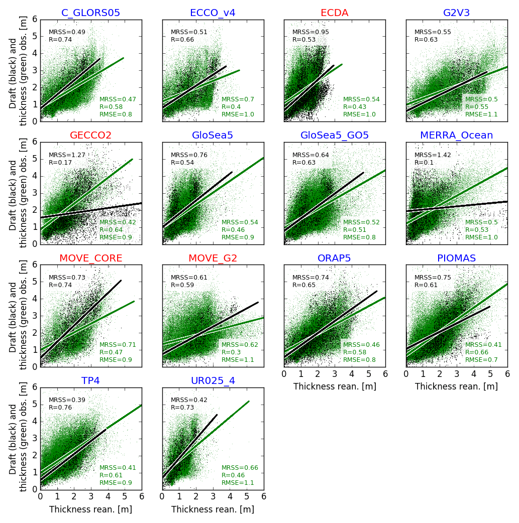
Figure 4Comparison between sea ice thickness from reanalyses and sea ice thickness (green points) or draft (black points) from observational datasets. The lines represent the linear fits having the reanalysis as the predictor and the observations as predicted variables. The mean residual sum of squares (MRSS) from the fit, the correlation coefficient (R), and the root mean square error (RMSE) are also displayed for each comparison. RMSE is calculated only when comparing SIT from both sources (green) but not when comparing SIT and draft (black). Reanalyses labeled in blue and red highlight whether the datasets were built with or without sea ice data assimilation, respectively.
3.2 Comparison of reanalyses to each other
As a first assessment of how well the reanalyses compare to each other, we estimate the RMSE and R between time series of the SIT anomaly, at every grid point, and between all pairs of products. The results are organized as a square matrix in Fig. 5, in which the number at the top of each panel represents the respective global value estimated by considering the data from all grid points. The lower triangular part of the matrix reveals that the smallest RMSE is found for the pair ECDA–UR025-4 (RMSE =0.21 m). Only four other pairs present RMSE ≤0.25; they are the match between the two GloSea5 products (0.23 m) and the combination of UR025-4 with C-GLORS05 and ECCO-v4 (0.25 m). The largest RMSE is found when comparing GECCO2–MOVE-G2 (0.61 m).
From Fig. 5 (lower triangle), the averaged RMSE for each individual reanalyses indicates that UR025-4 is the reanalysis closer to the ensemble, while MOVE-G2 has the largest errors compared to its counterparts: UR025-4 (0.30±0.06 m), ECCO-v4 (0.33±0.06 m), ECDA (0.33±0.06 m), GloSea5 (0.34±0.07 m), C-GLORS05 (0.35±0.06 m), PIOMAS (0.35±0.06 m), MOVE-CORE (0.36±0.06 m), GloSea5-GO5 (0.36±0.07 m), TOPAZ4 (0.37±0.06 m), ORAP5 (0.38±0.06 m), G2V3 (0.41±0.06 m), MERRA-Ocean (0.44±0.04 m), GECCO2 (0.45±0.06 m), and MOVE-G2 (0.47±0.06 m).

Figure 5Square matrix plot displaying the root mean square error (RMSE) (a) and the correlation coefficient (R) maps (b), estimated from the sea ice thickness time series, at every grid point, and between all pairs of reanalyses. The numbers at the top of each panel indicate the respective value calculated with data from all grid points. All maps have the 0∘ longitude placed at 06:00, while the bounding latitude is 67∘ N. Reanalyses labeled in blue and red highlight whether the datasets were built with or without ice data assimilation, respectively.
At the regional scale, most of the pairs of reanalyses have larger differences off the coast of northern Greenland and to the north of the Canadian Archipelago, which are more pronounced in the MERRA-Ocean product. Almost all systems present minimum errors in the central Arctic Basin.
In turn, the upper triangular part of the matrix in Fig. 5 displays the linear relationship between pairs of reanalyses, quantified by the correlation coefficient. The strongest pan-Arctic correlations are observed for GloSea5–GloSea-G05 (R=0.69), ORAP5–UR025-4 (0.67), and G2V3–ORAP5 (0.65). MOVE-CORE and MOVE-G2 present a marked anti-correlation with several other reanalyses, mainly in the central Arctic Ocean. Such anti-correlation is also reflected in the sea ice volume anomalies shown in Fig. 1. Notice that negative anomalies in MOVE-CORE and MOVE-G2, for instance from 2001 to 2004, occur at the same time that strong positive anomalies in reanalyses such as GECCO2, G2V3, and ECDA do, as well as C-GLORS05, ORAP5, PIOMAS, TOPAZ4, and UR025-4, though in a less pronounced way (Figs. 1 and 5). We do not have a clear understanding of why these anti-correlations take place.

Figure 6The e-folding timescales (or persistence) estimated for the SIT time series. Only grid cells in which the time mean (for the January 1993–December 2007 period) SIT at the time of summer minimum is greater than 0.1 m are taken into account for the computations. Averages for the systems with ice data assimilation and no data assimilation are represented by the DA and NA panels, respectively. All maps have the 0∘ longitude placed at 06:00, while the bounding latitude is 67∘ N. Reanalyses labeled in blue and red highlight whether the datasets were built with or without ice data assimilation, respectively.
3.3 Timescales
An important property inherent to time series in general concerns their timescale and/or persistence, as defined in Sect. 2.3. In other words, we aim to infer how long the SIT anomaly maintains a good correlation with future measurements at the same grid cell. Persistence can also be perceived as the skill of a self-prediction scheme, for which past data are used to predict future values. In addition, it is a relevant variable to be taken into account when designing the sampling frequency of observational programs, especially if these programs target the understanding of the SIT time variability.
Figure 6 displays the e-folding timescales for the SIT anomaly at every grid point, and for all reanalyses. The area weighted mean (AWM) timescales (in months) sorted in ascending order are 2.5 (GloSea5), 2.6 (GloSea5-GO5), 3.6 (PIOMAS) 3.7 (ECCO-v4), 3.8 (MERRA-Ocean), 4.0 (UR025-4), 4.3 (TOPAZ4), 4.4 (C-GLORS05), 4.7 (ORAP5), 4.9 (MOVE-CORE), 5.0 (G2V3), 6.0 (ECDA), 7.2 (MOVE-G2), and 7.8 months (GECCO2). These values were calculated only taking into account grid points with a valid SIT value from all reanalyses.
The results reveal that the thickness anomalies from reanalyses with no ice data assimilation (NA; Fig. 6, red labels) present a longer persistence, mainly distinguished in MOVE-G2 and GECCO2. Potential reasons to explain why the thickness anomalies persist longer in NA systems are suggested and discussed in Sect. 4. In contrast, the thickness anomalies from the GloSea5 systems (GloSea5 and GloSea5-GO5) have a much shorter persistence.
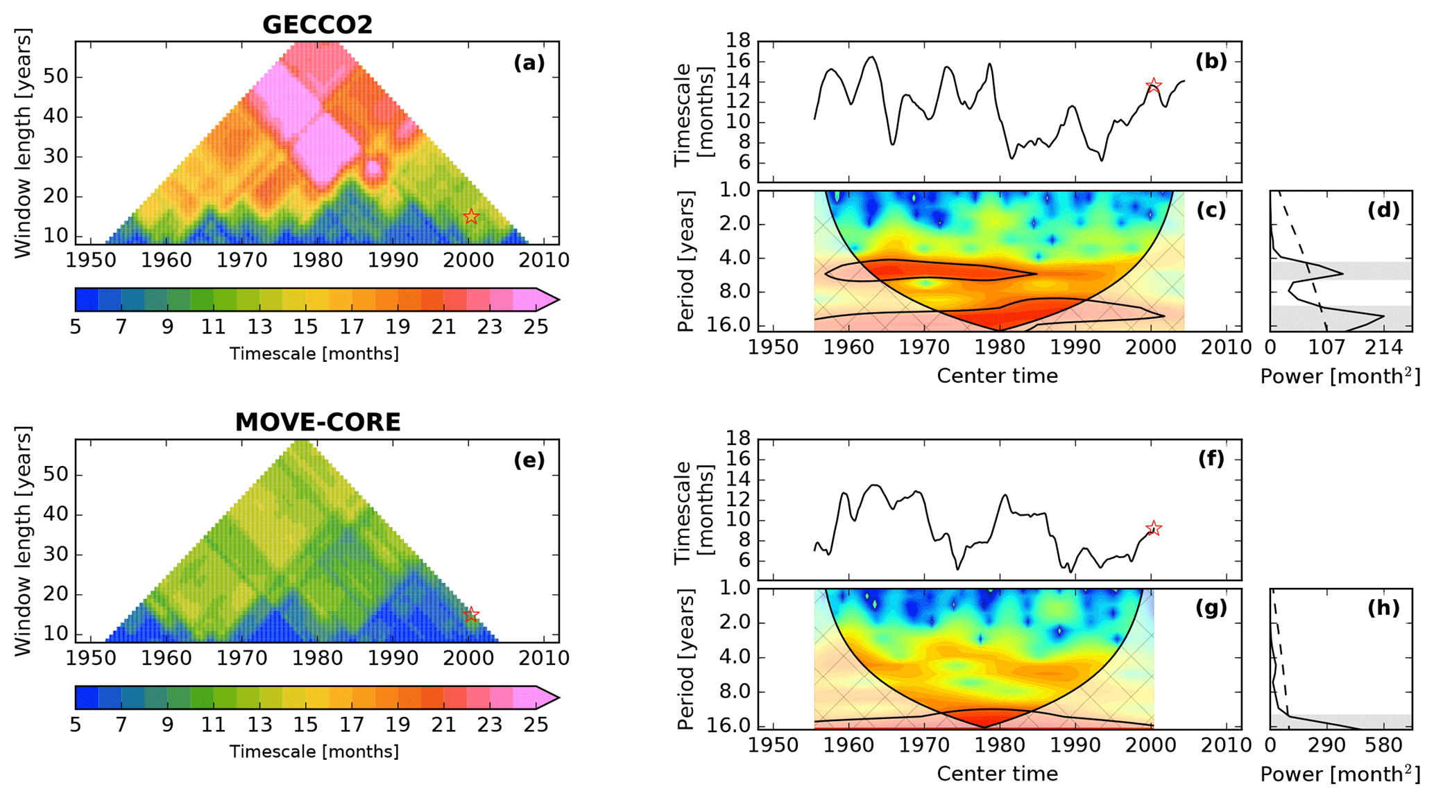
Figure 7(a) Moving e-folding timescales estimated for the ice volume anomaly time series from the GECCO reanalysis. The window length varies from 5 to 59 years, and it is stepped forward by 1 month over a total period of 64 years (January 1948–December 2011). (b) Moving e-folding timescales for the 15-year window length case. The red stars in (a) and (b) indicate the 15-year overlapping period (January 1993–December 2007, center time mid-June 2000). (c) Wavelet power spectrum of (b), with Morlet as the mother wavelet. The black lines denote the 95 % significance levels above a red noise background spectrum, while the crosshatched areas indicate the cone of influence, in which the edge effects become important. The color bar is omitted in panel (c) since we are not interested in the power's magnitude but in the frequencies outstanding as significant in the spectrum. (d) Time-integrated power spectrum from the wavelet analysis, where the dashed line corresponds to the 95 % significance level. The bands of significant periods (4.4–6.1 years and >10.7 years) are highlighted by the gray horizontal bars. (e)–(h) Same as (a)–(d), respectively, but for the MOVE-CORE ice volume anomaly which has a spanning period of 60 years (January 1948–December 2007). The horizontal gray bar in (h) highlights the only period band of significant variability, defined by periods longer than 12.7 years.
From a regional point of view, Fig. 6 shows that GloSea5 and GloSea5-G05 are the only reanalyses in which the SIT anomaly persistence is remarkably short all over the Arctic, presenting e-folding timescales higher than 4 months only in a few, not evenly distributed, grid points. By contrast, the SIT from GECCO2 has a marked longer persistence (>15 months) extending from the region off the northern coast of Greenland to the north of the Canadian Archipelago and mid-Arctic Ocean. The ECDA product presents a relatively similar pattern of the timescale over the region mentioned above but persisting for a shorter period (∼8 months). SIT anomalies from MOVE-G2 also indicate long persistence off the coast of northern Greenland, extending to the central Arctic and East Siberian Sea. For the remaining reanalyses, there is no common regional pattern of persistence outstanding from their respective timescale maps.
Nevertheless, the results above should be interpreted with caution. The e-folding timescale is a metric that depends on the shape of the lagged autocorrelation curve, which in turn may differ according to the period and time span of the original time series being analyzed. In order to evaluate how stable the timescale is by varying the time span and also by allowing it to evolve over time, we applied a time-moving and length-variable window to calculate the e-folding timescale of the ice volume anomaly (detrended in the same way as the SIT time series) from the two longest reanalyses (GECCO2 and MOVE-CORE), as shown in Fig. 7a and e. The window length varies from 5 to 59 years (stepped by 1 year) and it moves in time, stepped forward by 1 month. Here, we use the ice volume anomaly, rather than the SIT anomaly, for two reasons, first, because it is computationally more efficient than calculating the timescale for the SIT anomalies at every grid cell, considering the large number of interactions for a time-moving and length-variable window, and second, because the volume provides a pan-Arctic perspective of the SIT persistence.
Notice in Fig. 7a and e that the persistence overall grows to longer than ∼20 months when taking into account long time spans, remarkably for GECCO2 in which the ice volume anomaly persists for longer than 25 months at several center times. As for the thickness anomalies, MOVE-CORE presents a shorter persistence compared to GECCO2.
As a measure of stability, we estimate the standard deviations for all computations displayed in Fig. 7a and e. Results show that MOVE-CORE has a more stable timescale, with standard deviation of 3.0 months from its mean (9.7 months), while GECCO2 presents the average and standard deviation of 15.0±6.5 months.
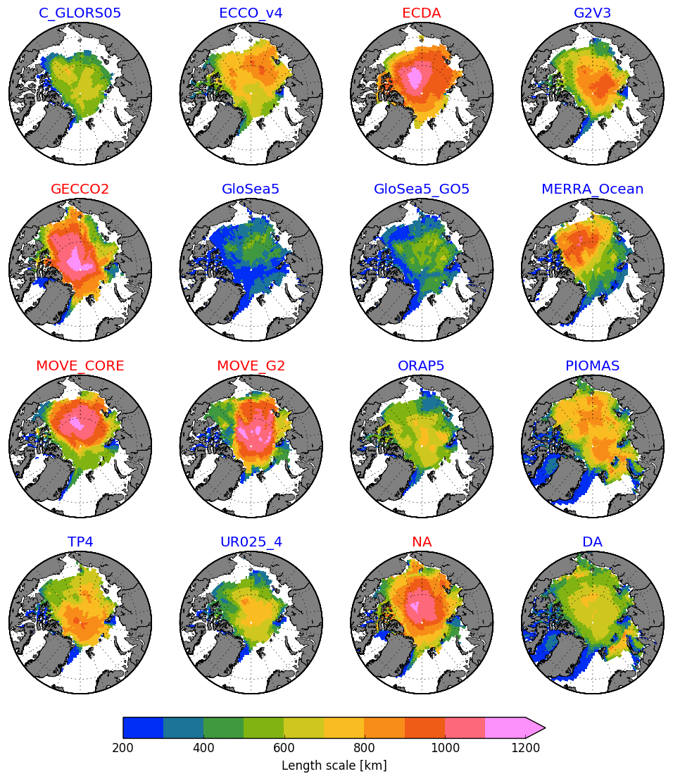
Figure 8The e-folding length scales estimated for the SIT time series. Only grid cells in which the time-mean (for the January 1993–December 2007 period) SIT at the time of summer minimum is greater than 0.1 m are taken into account for the computations. Averages for the systems with ice data assimilation and no data assimilation are represented by the DA and NA panels, respectively. All maps have the 0∘ longitude placed at 06:00, while the bounding latitude is 67∘ N. Reanalyses labeled in blue and red highlight whether the datasets were built with or without ice data assimilation, respectively.
Figure 7b and f show the case where the window length is 15 years, as it is for the overlapping period January 1993–December 2007. For this case, the average (standard deviation) timescales for GECCO2 and MOVE-CORE are 11.4±2.6 and 9.1±2.5 months, respectively. Minimum to maximum ranges are 6.2–16.5 months for GECCO2 and 4.9–13.5 months for MOVE-CORE. If we take into account the same center time of the time span January 1993–December 2007, that is mid-June 2000, the ice volume anomaly persistence is 13.6 and 9.2 months (red stars in Fig. 7b and f, respectively). Note that the timescales of the ice volume anomalies are a few months longer compared to the persistence of the AWM thickness anomalies (9.2 months, GECCO2; 5.4 months, MOVE-CORE).
We make use of wavelet analysis (Torrence and Compo, 1998) to evaluate whether the time series displayed in Fig. 7b and f exhibit a significant band(s) of variability. Figure 7c and d reveal that the ice volume anomaly from GECCO2 presents two bands of significant variability, as highlighted by the horizontal gray bars in Fig. 7d. The first spans from 4.4 to 6.1 years, and it is present in the first half of the time series but does not persist over time (black contours in Fig. 7c). The second is marked by periods longer than 10.7 years, which seems to be recurrent over time but should be interpreted with caution since it is placed near the “cone of influence”, in which edge effects become important, as indicated by crosshatched areas overlapping the black contours in Fig. 7c. The ice volume anomaly from MOVE-CORE, in turn, is marked by a single band of significant variability, with periods longer than 12.7 years (Fig. 7g, h). Again, this band should be interpreted with caution since it is also placed near the cone of influence.
3.4 Length scales
The e-folding length scale is a metric used for indicating how well a variable from a certain grid cell compares to the neighboring cells. In other words, it shows how the anomalies spread in space. As for the timescale, the length scale is a promising parameter to be explored when designing observational systems, but in terms of spatial coverage of instruments. Simplistically, regions marked with high length scales would require fewer instruments to be monitored better.
Figure 8 shows the length scales for the SIT anomaly at every grid point. The AWM length scales, in kilometers and ascending order, for each system are 337.0 (GloSea5), 420.7 (GloSea5-GO5), 544.6 (C-GLORS05), 681.5 (MERRA-Ocean), 724.3 (TOPAZ4), 728.2 (G2V3), 596.9 (ORAP5), 597.4 (UR025-4), 730.2 (PIOMAS), 732.5 (ECCO-v4), 846.7 (MOVE-G2), 835.8 (MOVE-CORE), 934.0 (ECDA), and 935.7 km (GECCO2).
A similar pattern to the timescale is observed here, with GloSea5 and GloSea5-GO5 presenting the minimum length scales, rarely higher than 500 km, while the reanalyses without sea ice data assimilation are characterized by higher length scales, sometimes higher than 1200 km. In all systems the length scales are relatively longer near the central Arctic. This suggests that higher length scales could be somehow associated with thicker ice. The relationships between mean ice thickness, timescale, and length scale will be explored in detail in Sect. 4.
The stability of the length scale over time (Fig. 9) was tested by means of a moving window with 15 years length, as follows: first, we calculate the one-point correlation maps for every grid point; second, we estimate the length scale for each one-point correlation map; third, the AWM length scale was calculated taking into account only grid points with a valid SIT value from all reanalyses; fourth, the process was repeated by stepping forward the 15-year window by 12 months. It is worthwhile mentioning that, computationally, it is much more expensive to calculate the length scale than the timescale. This is the reason why, here, we just use a time-moving but not length-variable window. The results suggest that the length scale is relatively more stable than the timescale (Fig. 7b and f), as further discussed in Sect. 4.
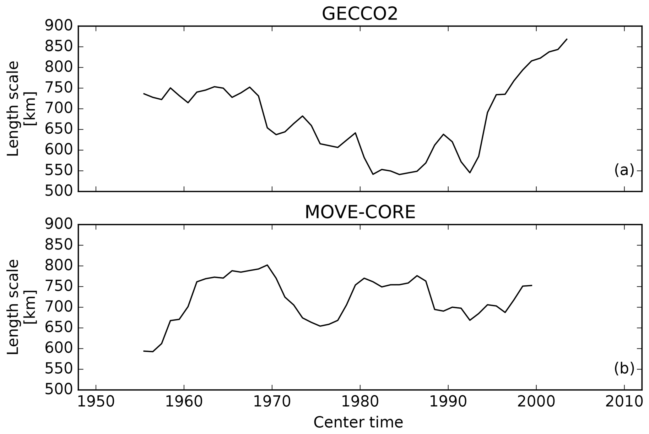
Figure 9(a) Moving e-folding length scales estimated for the ice volume anomaly time series from the GECCO reanalysis. The window length is 15 years, and it is stepped forward by 12 months over a total period of 64 years. (b) Same as (a), but for the MOVE-CORE reanalysis, which has a time span of 60 years.
The first aim of this study was to evaluate how the SIT from the reanalyses compares against observational datasets, either draft or SIT. We have used three different metrics to perform this comparison: the correlation coefficient (R), as a measure of the linear correlation between datasets; the mean residual sum of squares (MRSS), as an indicator of whether reanalysis values are good predictors for the observations; and the root mean square error (RMSE), which directly compares how the SIT from the reanalyses approaches the SIT from observations. The results show that some of the reanalyses have a relatively good correspondence either comparing SIT and draft or SIT from both sources of data. This is the case, for instance, for the TOPAZ4 product. A direct comparison between SIT from all reanalyses and observations indicates RMSEs ranging from 0.7 to 1.1 m. PIOMAS has the best agreement with the observational datasets. A particular case is GECCO2, which presents a relatively small RMSE and a good correlation with the SIT observational datasets, as well as a linear relationship. However, this same product is weakly correlated with the draft observational datasets as well as having poor predictive skill.
One of our main goals in performing such a comparison was to identify whether or not systems built with assimilation of sea ice concentration data are closer to observations, compared to the products built with no sea ice data assimilation. The results suggest that reanalyses with sea ice data assimilation do not necessarily perform better. One could speculate that some reanalyses do not reflect the covariances between sea ice concentration and SIT well.
We have compared the mean state (mean SIV) and respective variability (SD SIV) of all reanalyses against the specifications and parameters displayed in Table 1. Nevertheless, for such a comparison, where each system has its own configuration with several varying parameters, we were not able to distinguish the effect that the selected parameters may have on the mean state and variability. The comparison among SIT from the different reanalyses (Sect. 3.2) is not straightforward and does not necessarily improve due to common specifications and key parameters from the two systems being compared. For instance, the pair C-GLORS05–G2V3 shares a set of common assumptions (ocean–sea ice model, atmospheric forcing, vertical discretization, number of ice thickness categories, EVP dynamics, ocean–ice drag coefficient, analysis window, and both assimilate sea ice data), but this pair still presents a relatively high RMSE (0.39 m) and not such a strong correlation (R=0.4), as shown in Fig. 5. Only a few different assumptions and parameters, as well as their nonlinear interactions, may result in systems with considerably distinct mean state and variability. Although the pair C-GLORS05–G2V3 shares several common aspects, these two systems assume different air–ice drag coefficient and also assimilate the sea ice data in a different way, for instance. The same statement could be applied to other pairs of systems, e.g., G2V3–ORAP5, which also share some similarities but are still distinct in terms of mean state and variability.
The pair with the smallest RMSE (Fig. 5), ECDA–UR025-4, at the same time has a weak linear relationship (R=0.21). This reinforces the importance of looking at different metrics when comparing different products. If we average the RMSEs that one specific reanalysis presents against all the others (Fig. 5), thus comparing with the pan-Arctic mean ice volume of this same reanalysis, it becomes clear that products with relatively low sea ice volume (i.e., thin ice) present small RMSEs when compared with their counterparts (Fig. 10), although MERRA-Ocean is an outlier in this pattern by presenting thin sea ice but a large RMSE compared to the other reanalyses (Fig. 10, left upper corner). Figure 10 helps to explain why ECDA and UR025-4 have a small RMSE, though their anomalies are marked by a relatively weak correlation, as suggested in Fig. 5. This is also evident in the respective sea ice volume anomalies from these two reanalyses shown in Fig. 1. In the same way, Fig. 5 also indicates that the large differences in the SIT field take place near the coast of northern Greenland and the Canadian Archipelago, which are regions marked by the thickest sea ice over the studied domain.
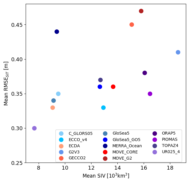
Figure 10Time-mean sea ice volume vs. the mean RMSE. This last parameter is an average of the RMSEs that each reanalysis has when its SIT field is compared individually to the other 13 reanalyses, as shown in Fig. 5. Shades of blue and purple indicate the reanalyses which do assimilate sea ice data, while shades of red indicate the reanalyses without sea ice data assimilation.
Another main goal of this work was to characterize the timescales and length scales of the sea ice thickness anomaly as well as to report whether these parameters are influenced by the fact that a respective reanalysis assimilates sea ice data or not. In this case, sea ice data assimilation plays a clear role in the scales referred to: systems with sea ice data assimilation are characterized by shorter timescales and length scales compared to the systems which do not assimilate sea ice data. Nevertheless, a comparison between the same system but built with (G2V3) and without (G2V1; not included in the 14 reanalyses of the present study) assimilation of sea ice concentration data (Fig. 11) suggests that this finding is valid in terms of pan-Arctic averages but not necessarily at every grid cell. This may explain why in the specific location addressed in Fig. 2 the reanalyses with data assimilation showed relatively longer timescales compared to the reanalyses without data assimilation. The pan-Arctic AWM timescale and AWM length scale from G2V3 are 5 months and 728.2 km, respectively. Without sea ice data assimilation (G2V1), the AWM timescale and AWM length scale increase to 5.5 months and 745.3 km, respectively.
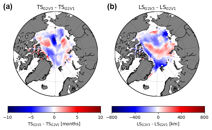
Figure 11Grid-point differences (G2V3–G2V1) of timescale (a) and length scale (b) between two versions of the GLORYS system: G2V3 which assimilates sea ice data and G2V1 which does not assimilate sea ice data.
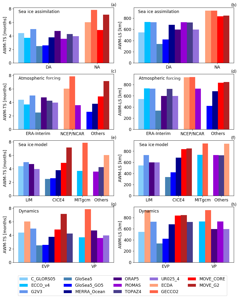
Figure 12Histograms showing how the AWM timescale (left-hand panels) and AWM length scale (right-hand panels) are related to different reanalysis specifications: (a–b) whether or not the system assimilates sea ice data, (c–d) the source of atmospheric forcing data, (e–f) the sea ice model used, and (g–h) the dynamics used (viscous–plastic or elastic–viscous–plastic) for ice–ice interactions that control ice deformation. Shades of blue and purple indicate the reanalyses which do assimilate sea ice data, while shades of red indicate the reanalyses without sea ice data assimilation.
Likely, the main reason why the assimilation of sea ice concentration data impacts the timescales and length scales of the SIT field is linked to the fact that when a reanalysis assimilates sea ice information, the system is forced towards the assimilated conditions, different from what occurs with free-running models. Eventually, data assimilation introduces SIT increments that are not necessarily physical and so contributes to an attenuation in the correlation of this variable at a certain grid cell both in time, with their future estimations, and in space, with the neighboring grid points.
We have shown that timescales and length scales are clearly influenced by whether or not the reanalyses assimilate sea ice data, as represented graphically in Fig. 12a–b. However, are these two properties also clearly influenced by other specifications and parameters? Figure 12c–h show how timescales and length scales are linked to the choices of atmospheric forcing, sea ice model, and dynamics for ice–ice interactions that control ice deformation (VP or EVP). Even though the atmospheric forcing fields are reported to play a major role in the sea ice simulations (Gerdes and Köberle, 2007; Rothrock and Wensnahan, 2007a), we could not identify distinguished patterns between the two main sources of atmospheric forcing used by the ensemble of reanalyses: ERA-Interim and NCEP/NCAR (Fig. 12c–d). Likewise, timescales and length scales are not clearly linked to the choices of sea ice model (Fig. 12e–f) and ice deformation dynamics (Fig. 12g–h), although a certain coherence in the timescales and length scales is observed for the systems that use the Louvain-la-Neuve sea ice model (LIM; Fig. 12e–f).
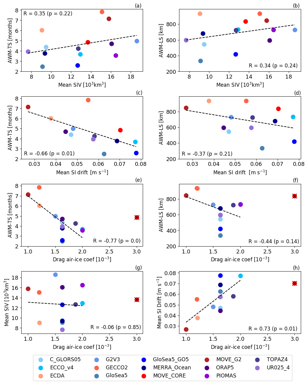
Figure 13Scatter plots showing how the (a, c, e) AWM timescale and (b, d, f) AWM length scale are related to the (a, b) mean state, (c, d) mean sea ice (SI) drift, and (e, f) drag air–ice coefficient. (g) Relation between drag air–ice coefficient and mean state. (f) Relation between drag air–ice coefficient and mean sea ice drift. Black dashed lines indicate the linear fit, while the coefficient of correlation R (and its respective p value) is also displayed in each panel. The black cross in panels (e)–(h) indicate that MOVE-CORE was not used in the respective regressions (black dashed lines), since this reanalysis adopts a much higher drag air–ice coefficient compared to the other 13 reanalyses. Shades of blue and purple indicate the reanalyses which do assimilate sea ice data, while shades of red indicate the reanalyses without sea ice data assimilation.
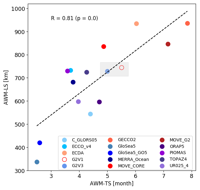
Figure 14Scatter plot of the average weighted mean (AWM) timescale vs. the AWM length scale. The black dashed line indicates the linear regression between both parameters, while the coefficient of correlation (R) is also displayed in the plot. The gray rectangle compares the two GLORYS systems: G2V1, built without sea ice data assimilation, and G2V3, built with sea ice data assimilation
Besides the spread among the points, the scatter plots displayed in Fig. 13a–b indicate a certain correlation between the time-mean SIV (mean state) and the studied scales, where relatively thin ice leads to shorter scales, in agreement with Massonnet et al. (2018). In contrast, the timescales have a marked anti-correlation with the sea ice drift as shown in Fig. 13c: reanalyses with faster sea ice present a short timescale. Such correlation is less pronounced for the length scale (Fig. 13d). Different parameters from the reanalyses could potentially influence the sea ice velocity. For instance, high air–ice and low ocean–ice drag coefficients each contribute to faster ice velocities (Tandon et al., 2018). As an example, ECCO-v4 has the second highest air–ice (smaller only compared to MOVE-CORE) and the smallest ocean–ice drag coefficients (see Table 1). This may explain why ECCO-v4 has relatively high ice velocities (Fig. 13c) and, therefore, low timescales and length scales (Figs. 6 and 8). For our ensemble of reanalyses, Fig. 13e shows a close correlation between sea ice velocity and the drag air–sea coefficients. Again, this correlation is less pronounced for the length scale (Fig. 13f).
The ice strength formulation is a major player in the sea ice velocity (Ungermann et al., 2017). All reanalyses follow the linear parameterization proposed by Hibler (1979), except the GloSea5 products and PIOMAS, which employ the ice strength formulation following Rothrock (1975). A higher ice strength parameter P* in Hibler's formulation leads to thicker and slower-moving ice, which would potentially lead to larger scales. Nevertheless, a relation between P* and the scales is not so clear for the ensemble of reanalyses (not shown). In addition, Ungermann et al. (2017) presented a detailed study comparing Hibler's and Rothrock's methods and showed that, for systems characterized by relatively thinner ice, model simulations with Rothrock's formulation result in lower ice strength, and therefore faster ice velocities, compared to Hibler's formulation. We do not have a clear understanding of why the GloSea5 products present such short timescales and length scales; however, we could speculate that the combination between relatively thin ice (Fig. 13a) and the use of Rothrock's ice strength formulation could support this result.
The discussion above indicates that timescales and length scales are mainly driven by the fact of whether or not the reanalyses assimilate sea ice data, but that they are also influenced by the air–ice drag coefficient and sea ice drift. Figure 14 shows a strong correlation between both timescales and length scales, whereby long timescales are associated with large length scales. Notice in this plot the difference in the timescales and length scales from G2V1 and G2V3 systems, highlighted by the gray rectangle placed near the center of the figure.
As mentioned before, the ice thickness timescales and length scales are interesting properties to be explored when designing and planning an optimal observation system both in terms of temporal sampling and spatial placement of instruments. Nevertheless, these properties also vary over time (Figs. 7 and 9). The stability over time of timescales and length scales can be estimated by the coefficient of variation (Cv= SD/Mean). The Cv is a non-dimensional metric used to evaluate the extent of a certain variability in relation to its mean, allowing different properties to be compared. The Cv for the GECCO2 and MOVE-CORE moving timescales, estimated from the time series shown in Fig. 7b and f, is 0.23 and 0.27, respectively, while the Cv for moving length scales (Fig. 9) is 0.13 and 0.07.
Lastly, it is worthwhile mentioning that both timescales and length scales are promising properties to support the design of an optimal observing system. As suggested by the Cv presented above, and by the fact that the timescale is more sensitive to the reanalysis specifications and parameters (see Fig. 13c–f), the length scale is considerably more stable than the timescale; therefore it is a more reliable variable to be taken into account for deploying observing systems. For instance, the multiple linear regression model used by Lindsay and Zhang (2006), for determining optimal locations to predict sea ice extent from SIT, could be combined with the length scale information, thereby avoiding two or more stations placed into the same radius of correlation (length scale) being selected. The timescale would be more useful if used in combination with the knowledge of its variability. Further studies are required to evaluate the performance of timescales and length scales in providing support for the optimal design of observational programs, though this work already shows some promising results in that direction.
All datasets used in this work are freely available, as follows: Reanalyses data are from https://icdc.cen.uni-hamburg.de/1/daten/reanalysis-ocean/oraip.html (University of Hamburg, 2019). PIOMAS is from http://psc.apl.uw.edu/research/projects/arctic-sea-ice-volume-anomaly/ (Zhang and Rothrock, 2003). Observational data are from http://psc.apl.uw.edu/sea_ice_cdr/ (Schweiger, 2017).
This appendix displays all abbreviations and their respective written-out names referred to in the text and used in the figures. The long names of some abbreviations were previously omitted in order to preserve the readability of text, while others were already defined. All of them will be mentioned below so that the reader can easily consult their meaning at any time.
| AER | Atmospheric and Environmental Research |
| AWI | Alfred Wegener Institute |
| AWM | Area-weighted mean |
| BIO-LS | Bedford Institute of Oceanography |
| Lancaster Sound | |
| BGEP | Beaufort Gyre Exploration Project |
| C-GLORS05 | CMCC – Global Ocean |
| Reanalysis System | |
| CDR | Climate Data Record |
| CHK | Chuck Sea |
| CMCC | Centro Euro-Mediterraneo sui |
| Cambiamenti Climatici | |
| CryoSat | CRYOgenic SATellite |
| Cv | Coefficient of variation |
| DAv | Data assimilation |
| EBS | Eastern Beaufort Sea |
| ECCO-v4 | Estimating the Circulation and Climate |
| of the Ocean – version 4 | |
| ECDA | Ensemble Coupled Data Assimilation |
| ECMWF | European Centre for Medium-Range |
| Weather Forecasts | |
| ESA | European Space Agency |
| EVP | Elastic–viscous–plastic |
| GECCO2 | German – Estimating the Circulation |
| and Climate of the Ocean | |
| GFDL | Geophysical Fluid Dynamics Laboratory |
| GLORYS | Global Ocean reanalysis and Simulation |
| GloSea5 | Global Seasonal forecasting system |
| GloSea5-GO5 | Global Seasonal forecasting system – |
| Global Ocean 5.0 | |
| GMAO | Global Modeling and Assimilation Office |
| GS | Greenland Sea |
| GSFC | Goddard Space Flight Center |
| G2V3 | GLORYS 2 – version 3 |
| ICESat | Ice, Cloud, and land Elevation Satellite |
| IOS | Institute of Ocean Science |
| JMA | Japan Meteorological Agency |
| JPL | Jet Propulsion Laboratory |
| MERRA | Modern Era Retrospective-analysis for |
| Research and Applications | |
| ARC MFC | Arctic Marine Forecasting Center |
| MIT | Massachusetts Institute of Technology |
| MOVE-CORE | Multivariate Ocean Variational Estimation – |
| Coordinated Ocean-ice Reference Experiment | |
| MOVE-G2 | Multivariate Ocean Variational Estimation – |
| Global version 2 | |
| MRI | Meteorological Research Institute |
| MRSS | Mean residual sum of squares |
| NAv | No data assimilation |
| NASA | National Aeronautics and Space Administration |
| NOAA | National Oceanic and Atmospheric Administration |
| NPEO | North Pole Environmental Observatory |
| ORA-IP | Ocean Reanalysis Intercomparison project |
| PIOMAS | Pan-Arctic Ice-Ocean Modeling and |
| Assimilation System | |
| R | Correlation coefficient |
| RMSE | Root mean square error |
| SIT | Sea ice thickness |
| TP4 | TOPAZ4 |
| UK-Subs-AN | UK Navy Submarines – Analog |
| UK-Subs-DG | UK Navy Submarines – Digital |
| ULS | Upward-looking sonar |
| US-Subs-AN | US Navy Submarines – Analog |
| US-Subs-DG | US Navy Submarines – Digital |
| UR025-4 | University of Reading, |
| deg – version 4 | |
| VP | Viscous–plastic |
| YOPP | Year Of Polar Prediction |
This appendix presents the comparison of all reanalysis products with all different observational datasets. This comparison is based on three different metrics: the root mean square error (RMSE), the mean residual sum of squares (MRSS), and the correlation coefficient (R).
Table B1Root mean square error (RMSE; in m) calculated between the SIT from observations and reanalyses.
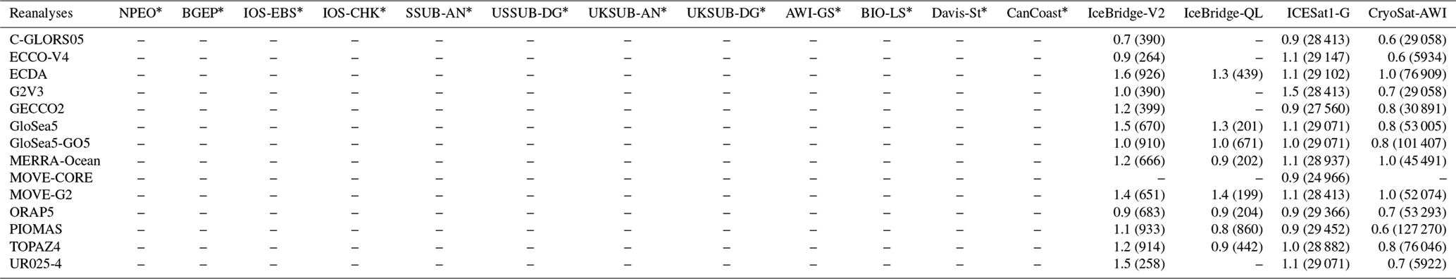
* The RMSE was not calculated for the draft datasets.
Table B2Mean residual sum of squares (MRSS; in m2) estimated from the linear fit between the SIT from reanalysis (predictor) and observations (predicted), either draft or SIT, respectively.

* Draft observational datasets are distinguished from the SIT datasets.
Table B3Correlation coefficient (R) estimated between the SIT from reanalysis and observations, either draft or SIT.

* Draft observational datasets are distinguished from the SIT datasets.
LP, FM, MC and TF designed the science plan. LP processed the data and plotted the figures. LP analyzed the results and wrote the manuscript based on insights from all co-authors.
The authors declare that they have no conflict of interest.
The work presented in this paper has received funding from the European Union's Horizon 2020 Research and Innovation
programme under grant agreement no. 727862: APPLICATE project (Advanced prediction in Polar regions and beyond).
David Docquier is funded by the EU Horizon 2020 PRIMAVERA project, grant agreement no. 641727.
We thank two anonymous reviewers for their constructive suggestions and criticism.
We thank Axel Schweiger for making the observational dataset available by means of the Unified Sea Ice Thickness Climate
Data Record (http://psc.apl.uw.edu/sea_ice_cdr; last access: 15 July 2018) and also for kindly making some aspects of the data clear.
The BGEP data used in Fig. 2 were collected and made available by the Beaufort Gyre Exploration Project based at the
Woods Hole Oceanographic Institution (http://www.whoi.edu/beaufortgyre; last access: 15 July 2018).
The Python wavelet software is provided by Evgeniya Predybaylo based on
Torrence and Compo (1998) and is available at
http://atoc.colorado.edu/research/wavelets/ (last access: 15 July 2018).
Edited by: Dirk Notz
Reviewed by: two anonymous referees
Anisimov, O. A., Vaughan, D. G., Callaghan, T. V., Furgal, C., Marchant, H., Prowse, T. D., Vilhjálmsson, H., and Walsh, J. E.: Polar regions (Arctic and Antarctic), Climate Change 2007: Impacts, Adaptation and Vulnerability, Contribution of Working Group II to the Fourth Assessment Report of the Intergovernmental Panel on Climate Change, Cambridge University Press, Cambridge, 2007. a
Balmaseda, M. A., Hernandez, F., Storto, A., Palmer, M. D., Alves, O., Shi, L., Smith, G. C., Toyoda, T., Valdivieso, M., Barnier, B., Behringer, D., Boyer, T., Chang, Y.-S., Chepurin, G. A., Ferry, N., Forget, G., Fujii, Y., Good, S., Guinehut, S., Haines, K., Ishikawa, Y., Keeley, S., Köhl, A., Lee, T., Martin, M. J., Masina, S., Masuda, S., Meyssignac, B., Mogensen, K., Parent, L., Peterson, K. A., Tang, Y. M., Yin, Y., Vernieres, G., Wang, X., Waters, J., Wedd, R., Wang, O., Xue, Y., Chevallier, M., Lemieux, J.-F., Dupont, F., Kuragano, T., Kamachi, M., Awaji, T., Caltabiano, A., Wilmer-Becker, K., and Gaillard, F.: The Ocean Reanalyses Intercomparison Project (ORA-IP), J. Oper. Oceanogr., 8, s80–s97, https://doi.org/10.1080/1755876X.2015.1022329, 2015. a
Blanchard-Wrigglesworth, E. and Bitz, C.: Characteristics of Arctic Sea-Ice Thickness Variability in GCMs, J. Climate, 27, 8244–8258, https://doi.org/10.1175/JCLI-D-14-00345.1, 2014. a, b, c, d, e, f, g
Blanchard-Wrigglesworth, E., Armour, K. C., Bitz, C., and DeWeaver, E.: Persistence and Inherent Predictability of Arctic Sea Ice in a GCM Ensemble and Observations, J. Climate, 24, 231–250, https://doi.org/10.1175/2010JCLI3775.1, 2011. a, b, c
Blockley, E. W., Martin, M. J., McLaren, A. J., Ryan, A. G., Waters, J., Lea, D. J., Mirouze, I., Peterson, K. A., Sellar, A., and Storkey, D.: Recent development of the Met Office operational ocean forecasting system: an overview and assessment of the new Global FOAM forecasts, Geosci. Model Dev., 7, 2613–2638, https://doi.org/10.5194/gmd-7-2613-2014, 2014. a
Budyko, M. I.: The effect of solar radiation variations on the climate of the Earth, Tellus, 21, 611–619, https://doi.org/10.1111/j.2153-3490.1969.tb00466.x, 1969. a
Chang, Y. S., Zhang, S., Rosati, A., Delworth, T. L., and Stern, W. F.: An assessment of oceanic variability for 1960–2010 from the GFDL ensemble coupled data assimilation, Clim. Dynam., 40, 775–803, https://doi.org/10.1007/s00382-012-1412-2, 2013. a
Chevallier, M. and Salas-Mélia, D.: The role of sea ice thickness distribution in the Arctic sea ice potential predictability: a diagnostic approach with a coupled GCM, J. Climate, 25, 3025–3038, https://doi.org/10.1175/JCLI-D-11-00209.1, 2012. a
Chevallier, M., Smith, G. C., Dupont, F., Lemieux, J.-F., Forget, G., Fujii, Y., Hernandez, F., Msadek, R., Peterson, K. A., Storto, A., Toyoda, T., Valdivieso, M., Vernieres, G., Zuo, H., Balmaseda, M., Chang, Y.-S., Ferry, N., Garric, G., Haines, K., Keeley, S., Kovach, R. M., Kuragano, T., Masina, S., Tang, Y., Tsujino, H., and Wang, X.: Intercomparison of the Arctic sea ice cover in global ocean-sea ice reanalyses from the ORA–IP project, Clim. Dynam, 19, 1107–1136, https://doi.org/10.1007/s00382-016-2985-y, 2017. a, b, c
Danabasoglu, G., Yeager, S. G., Bailey, D., Behrens, E., Bentsen, M., Bi, D., Biastoch, A., Boning, C., Bozec, A., Canuto, V., Cassou, C., Chassignet, E., Coward, A. C., Danilov, S., Diansky, N., Drange, H., Farneti, R., Fernandez, E., Fogli, P. G., Forget, G., Fujii, Y., Griffies, S. M., Gusev, A., Heimbach, P., Howard, A., Jung, T., Kelley, M., Large, W. G., Leboissetier, A., Lu, L., Madec, G., Marsland, S. J., Masina, S., Navarra, A., Nurser, A. J. G., Pirani, A., Salas-Melia, D., Samuels, B. L., Scheinert, M., Sidorenko, D., Treguier, A. M., Tsujino, H., Uotila, P., Valcke, S., Voldoire, A., and Wang, Q.: North Atlantic simulations in Coordinated Ocean-ice Reference Experiments phase II (CORE-II). Part I: Mean states, Ocean Model., 73, 76–107, https://doi.org/10.1016/j.ocemod.2013.10.005, 2014. a
Day, J. J., Tietsche, S., and Hawkins, E.: Pan-Arctic and Regional Sea Ice Predictability: Initialization Month Dependence, J. Climate, 27, 4371–4390, https://doi.org/10.1175/JCLI-D-13-00614.1, 2014. a
Drange, H. and Simonsen, K.: Formulation of air-sea fluxes in the ESOP2 version of MICOM, Technical Report No. 125, Tech. rep., Nansen Environmental and Remote Sensing Center, 1996.
Drijfhout, S.: Competition between global warming and an abrupt collapse of the AMOC in Earth's energy imbalance, Sci. Rep.-UK, 5, 1–12, https://doi.org/10.1038/srep14877, 2015. a
Drucker, R., Martin, S., and Moritz, R.: Observations of ice thickness and frazil ice in the St. Lawrence Island polynya from satellite imagery, upward looking sonar, and salinity/temperature moorings, J. Geophys. Res., 108, 18-1–18-18, https://doi.org/10.1029/2001JC001213, 2003. a, b
Ferry, N., Parent, L., Garric, G., Barnier, B., and Jourdain, N. C.: Mercator global Eddy permitting ocean reanalysis GLORYS1V1: description and results, Mercator-Ocean Q. Newslett., 36, 15–27, 2010. a
Forget, G., Campin, J.-M., Heimbach, P., Hill, C. N., Ponte, R. M., and Wunsch, C.: ECCO version 4: an integrated framework for non-linear inverse modeling and global ocean state estimation, Geosci. Model Dev., 8, 3071–3104, https://doi.org/10.5194/gmd-8-3071-2015, 2015. a
Gerdes, R. and Köberle, C.: Comparison of Arctic sea ice thickness variability in IPCC Climate of the 20th Century experiments and in ocean-sea ice hindcasts, J. Geophys. Res., 112, C04S13, https://doi.org/10.1029/2006JC003616, 2007. a
Gleick, P. H.: The implications of global climatic changes for international security, Climatic Change, 15, 309–325, https://doi.org/10.1007/BF00138857, 1989. a
Guemas, V., Blanchard-Wrigglesworth, E., Chevallier, M., Day, J. J., Déqué, M., Doblas-Reyes, F. J., Fučkar, N. S., Germe, A., Hawkins, E., Keeley, S., Koenigk, T., Salas y Mélia, D., and Tietsche, S.: A review on Arctic sea-ice predictability and prediction on seasonal to decadal time-scales, Q. J. Roy. Meteor. Soc., 142, 546–561, https://doi.org/10.1002/qj.2401, 2016. a, b, c
Handorf, U.: Tourism booms as the Arctic melts. A critical approach of polar tourism, GRIN Verlag, Munich, 2011. a
Hansen, J., Sato, M., Hearty, P., Ruedy, R., Kelley, M., Masson-Delmotte, V., Russell, G., Tselioudis, G., Cao, J., Rignot, E., Velicogna, I., Tormey, B., Donovan, B., Kandiano, E., von Schuckmann, K., Kharecha, P., Legrande, A. N., Bauer, M., and Lo, K.-W.: Ice melt, sea level rise and superstorms: evidence from paleoclimate data, climate modeling, and modern observations that 2 ∘C global warming could be dangerous, Atmos. Chem. Phys., 16, 3761–3812, https://doi.org/10.5194/acp-16-3761-2016, 2016. a
Harms, S., Fahrbach, E., and Strass, V.: Sea ice transports in the Weddell Sea, J. Geophys. Res., 106, 9057–9073, https://doi.org/10.1029/1999JC000027, 2001. a
Hibler, W. D.: A dynamic thermodynamic sea ice model, J. Phys. Oceanogr., 9, 815–846, https://doi.org/10.1175/1520-0485(1979)009<0815:ADTSIM>2.0.CO;2, 1979. a
Holland, M. M. and Bitz, C. M.: Polar amplification of climate change in coupled models, Clim. Dynam., 21, 221–232, https://doi.org/10.1007/s00382-003-0332-6, 2003. a
Holland, M. M., Bailey, D. A., and Vavrus, S.: Inherent sea ice predictability in the rapidly changing Arctic environment of the Community Climate System Model, version 3, Clim. Dynam., 36, 1239–1253, https://doi.org/10.1007/s00382-010-0792-4, 2011. a
Hunke, E. C. and Dukowicz, J. K.: An elastic-viscous-plastic model for sea ice dynamics, J. Phys. Oceanogr., 27, 1849–1867, https://doi.org/10.1175/1520-0485(1997)027<1849:AEVPMF>2.0.CO;2, 1997.
Jung, T., Gordon, N. D., Bauer, P., Bromwich, D. H., Chevallier, M., Day, J. J., Dawson, J., Doblas-Reyes, F., Fairall, C., amd M. Holland, H. F. G., Inoue, J., Iversen, T., Klebe, S., Lemke, P., Losch, M., Makshtas, A., Mills, B., Nurmi, P., Perovich, D., Reid, P., Renfrew, I. A., Smith, G., Svensson, G., Tolstykh, M., and Yang, Q.: Advancing polar prediction capabilities on daily to seasonal time scales, B. Am. Meteorol. Soc., 97, 1631–1647, https://doi.org/10.1175/BAMS-D-14-00246.1, 2016. a
Köhl, A.: Evaluation of the GECCO2 Ocean Synthesis: Transports of Volume, Heat and Freshwater in the Atlantic, Q. J. Roy. Meteor. Soc., 141, 166–181, https://doi.org/10.1002/qj.2347, 2015. a
Krishfield, R. A., Proshutinsky, A., Tateyama, K., Williams, W. J., Carmack, E. C., McLaughlin, F. A., and Timmermans, M. L.: Deterioration of perennial sea ice in the Beaufort Gyre from 2003 to 2012 and its impact on the oceanic freshwater cycle, J. Geophys. Res.-Oceans, 119, 1271–1305, https://doi.org/10.1002/2013JC008999, 2013. a
Krupnik, I. and Jolly, D.: Earth is Faster Now: Indigenous Observations of Arctic Environmental Change, Arctic Research Consortium of the United States, Fairbanks, Alaska, 2002. a
Kurtz, N. T., Farrell, S. L., Studinger, M., Galin, N., Harbeck, J. P., Lindsay, R., Onana, V. D., Panzer, B., and Sonntag, J. G.: Sea ice thickness, freeboard, and snow depth products from Operation IceBridge airborne data, The Cryosphere, 7, 1035–1056, https://doi.org/10.5194/tc-7-1035-2013, 2013. a
Lindsay, R. and Schweiger, A.: Arctic sea ice thickness loss determined using subsurface, aircraft, and satellite observations, The Cryosphere, 9, 269–283, https://doi.org/10.5194/tc-9-269-2015, 2015. a
Lindsay, R. W.: A new sea ice thickness climate data record, EOS, 91, 405–406, https://doi.org/10.1029/2010EO440001, 2010. a, b
Lindsay, R. W. and Zhang, J.: Arctic Ocean Ice Thickness: Modes of Variability and the Best Locations from Which to Monitor Them, J. Phys. Oceanogr., 36, 496–506, https://doi.org/10.1175/JPO2861.1, 2006. a
Lindsay, R. W., Zhang, J., Schweiger, A. J., and Steele, M. A.: Seasonal predictions of ice extent in the Arctic Ocean, J. Geophys. Res., 113, C02023, https://doi.org/10.1029/2007JC004259, 2008. a
Lindstad, H., Bright, R. M., and Strømmanb, A. H.: Economic savings linked to future Arctic shipping trade are at odds with climate change mitigation, Transp. Policy, 45, 24–34, https://doi.org/10.1016/j.tranpol.2015.09.002, 2016. a
Manabe, S. and Stouffer, R. J.: Sensitivity of a global climate model to an increase of CO2 in the atmosphere, J. Geophys. Res., 85, 5529–5554, https://doi.org/10.1029/JC085iC10p05529, 1980a. a
Manabe, S. and Stouffer, R. J.: Sensitivity of a global climate model to an increase of CO2 concentration in the atmosphere, J. Geophys. Res., 85, 5529–5554, https://doi.org/10.1029/JC085iC10p05529, 1980b. a
Massonnet, F., Vancoppenolle, M., Goosse, H., Docquier, D., Fichefet, T., and Blanchard-Wrigglesworth, E.: Arctic sea-ice change tied to its mean state through thermodynamic processes, Nat. Clim. Change, 8, 599–603, https://doi.org/10.1038/s41558-018-0204-z, 2018. a
Maykut, G. A.: Large-scale heat exchange and ice production in the central Arctic, J. Geophys. Res., 87, 7971–7984, https://doi.org/10.1029/JC087iC10p07971, 1982. a
Megann, A., Storkey, D., Aksenov, Y., Alderson, S., Calvert, D., Graham, T., Hyder, P., Siddorn, J., and Sinha, B.: GO5.0: the joint NERC-Met Office NEMO global ocean model for use in coupled and forced applications, Geosci. Model Dev., 7, 1069–1092, https://doi.org/10.5194/gmd-7-1069-2014, 2014. a
Mellor, G. L. and Kantha, L.: An ice-ocean coupled model, J. Geophys. Res., 94, 10937–10954, 1989.
Nelson, F. E., Anisimov, O. A., and Shiklomanov, N. I.: Climate Change and Hazard Zonation in the Circum-Arctic Permafrost Regions, Natural Hazards, 26, 203–225, https://doi.org/10.1023/A:1015612918401, 2002. a
Nuttall, M., Berkes, F., Forbes, B., Kofinas, G., Vlassova, T., and Wenzel, G.: Arctic Climate Impact Assessment, Cambridge University Press, Cambridge, 2005. a
Pettipas, R., Hamilton, J., and Prinsenberg, S.: Moored current meter and CTD observations from Barrow Strait, 2003–2004, Can. Data Rep. Hydrogr. Ocean Sci., 173, 134 pp., 2008. a
Prinsenberg, S. and Pettipas, R.: Ice and ocean mooring data statistics from Barrow Strait, the central section of the NW Passage in the Canadian Arctic Archipelago, Int. J. Offshore Polar, 18, 277–281, 2008. a
Prinsenberg, S., Hamilton, J., Peterson, I., and Pettipas, R.: Influence of climate change on the changing Arctic and Sub-Arctic conditions, edited by: Nihoul, J. and Kostianoy, A., Springer, Dordrecht, 2009. a
Ricker, R., Hendricks, S., Helm, V., Skourup, H., and Davidson, M.: Sensitivity of CryoSat-2 Arctic sea-ice freeboard and thickness on radar-waveform interpretation, The Cryosphere, 8, 1607–1622, https://doi.org/10.5194/tc-8-1607-2014, 2014. a
Rienecker, M. M., Suarez, M. J., Gelaro, R., Todling, R., Bacmeister, J., Liu, E., Bosilovich, M. G., Schubert, S. D., Takacs, L., Kim, G. K., Bloom, S., Chen, J., Collins, D., Conaty, A., da Silva, A., Gu, W., Joiner, J., Koster, R. D., Lucchesi, R., Molod, A., Owens, T., Pawson, S., Pegion, P., Redder, C. R., Reichle, R., Robertson, F. R., Ruddick, A. G., Sienkiewicz, M., and Woollen, J.: MERRA: NASA's Modern-Era Retrospective Analysis for Research and Applications, J. Climate, 24, 3624–3648, https://doi.org/10.1175/JCLI-D-11-00015.1, 2011. a
Rothrock, D. A.: The energetics of the plastic deformation of pack ice by ridging, J. Geophys. Res., 80, 4514–4519, https://doi.org/10.1029/JC080i033p04514, 1975. a
Rothrock, D. A. and Wensnahan, M.: Global atmospheric forcing data for Arctic ice-ocean modeling, J. Geophys. Res., 112, C04S14, https://doi.org/10.1029/2006JC003640, 2007a. a
Rothrock, D. A. and Wensnahan, M.: The Accuracy of Sea Ice Drafts Measured from U.S. Navy Submarines, J. Atmos. Ocean. Tech., 24, 1936–1949, https://doi.org/10.1175/JTECH2097.1, 2007b. a, b, c
Sakov, P., Counillon, F., Bertino, L., Lisæter, K. A., Oke, P. R., and Korablev, A.: TOPAZ4: an ocean-sea ice data assimilation system for the North Atlantic and Arctic, Ocean Sci., 8, 633–656, https://doi.org/10.5194/os-8-633-2012, 2012. a
Serreze, M. C., Barrett, A. P., Stroeve, J. C., Kindig, D. N., and Holland, M. M.: The emergence of surface-based Arctic amplification, The Cryosphere, 3, 11–19, https://doi.org/10.5194/tc-3-11-2009, 2009. a
Sévellec, F., Fedorov, A. V., and Liu, W.: Arctic sea-ice decline weakens the Atlantic Meridional Overturning Circulation, Nat. Clim. Change, 7, 604–610, https://doi.org/10.1038/nclimate3353, 2017. a
Schweiger, A. J.: Unified Sea Ice Thickness Climate Data Record, available at: http://psc.apl.uw.edu/sea_ice_cdr/ (last access: 13 Februiary 2019), 2017.
Storto, A., Masina, S., and Dobricic, S.: Estimation and Impact of Nonuniform Horizontal Correlation Length Scales for Global Ocean Physical Analyses, J. Atmos. Ocean. Tech., 31, 2330–2349, https://doi.org/10.1175/JTECH-D-14-00042.1, 2014. a
Stroeve, J. C., Hamilton, L., Blitz, C. M., and Blanchard-Wrigglesworth, E.: Predicting September sea ice: Ensemble skill of the SEARCH sea ice outlook 2008–2013, Geophys. Res. Lett., 41, 2411–2418, https://doi.org/10.1002/2014GL059388, 2014. a
Tandon, N. F., Kushner, P. J., Docquier, D., Wettstein, J. J., and Li, C.: Reassessing Sea Ice Drift and its Relationship to LongTerm Arctic Sea Ice Loss in Coupled Climate Models, J. Geophys. Res., 123, 4338–4359, https://doi.org/10.1029/2017JC013697, 2018. a
Tietsche, S., Balmaseda, M. A., Zuo, H., and Mogensen, K.: Arctic sea ice in the global eddy-permitting ocean reanalysis ORAP5, ECMWF technical memorandum, 49, 775–789, https://doi.org/10.1007/s00382-015-2673-3, 2017. a
Torrence, C. and Compo, G. P.: A practical guide to wavelet analysis, B. Am. Meteorol. Soc., 79, 61–78, https://doi.org/10.1175/1520-0477(1998)079<0061:APGTWA>2.0.CO;2, 1998. a, b, c
Toyoda, T., Fujii, Y., Yasuda, T., Usui, N., Iwao, T., Kuragano, T., and Kamachi, M.: Improved Analysis of Seasonal-Interannual Fields Using a Global Ocean Data Assimilation System, Theor. Appl. Mech. Jpn., 61, 31–48, https://doi.org/10.11345/nctam.61.31, 2013. a
Tucker III, W. B., Weatherly, J. W., Eppler, D. T., Farmer, D., and Bentley, D. L.: Evidence for the rapid thinning of sea ice in the western Arctic Ocean at the end of the 1980s, Geophys. Res. Lett., 28, 2851–2854, https://doi.org/10.1029/2001GL012967, 2001. a
Ungermann, M., Tremblay, L. B., Martin, T., and Losch, M.: Impact of the ice strength formulation on the performance of a sea ice thickness distribution model in the Arctic, J. Geophys. Res., 122, 2090–2107, https://doi.org/10.1002/2016JC012128, 2017. a, b
University of Hamburg: The Ocean Reanalyses Intercomparison Project, available at: https://icdc.cen.uni-hamburg.de/1/daten/reanalysis-ocean/oraip.html, last access: 13 February 2019. a
Uotila, P., Goosse, H., Haines, K., Chevallier, M., Barthélemy, A., Bricaud, C., Carton, J., Fučkar, N., Garric, G., Iovino, D., Kauker, F., Korhonen, M., Lien, V. S., Marnela, M., Massonnet, F., Mignac, D., Peterson, K. A., Sadikni, R., Shi, L., Tietsche, S., Toyoda, T., Xie, J., and Zhang, Z.: An assessment of ten ocean reanalyses in the polar regions, Clim. Dynam., 1–38, https://doi.org/10.1007/s00382-018-4242-z, 2018. a
Valdivieso, M., Haines, K., Zuo, H., and Lea, D.: Freshwater and heat transports from global ocean synthesis, J. Geophys. Res., 119, 394–409, https://doi.org/10.1002/2013JC009357, 2014. a
Wadhams, P.: Arctic sea ice morphology and its measurement, Arctic Technology and Policy, edited by: Dyer, I. and Chryssostomidis, C., Hemisphere Publishing Corp., Washington, D.C., 1984. a
Wadhams, P. and Horne, R. J.: An analysis of ice profiles obtained by submarine in the Beaufort Sea, J. Glaciol., 25, 401–424, https://doi.org/10.3189/S0022143000015264, 1980. a
Walsh, J. E.: Intensified warming of the Arctic: Causes and impacts on middle latitudes, Global Planet. Change, 117, 52–63, https://doi.org/10.1016/j.gloplacha.2014.03.003, 2014. a
Wensnahan, M. and Rothrock, D. A.: Sea-ice draft from submarine-based sonar: Establishing a consistent record from analog and digitally recorded data, Geophys. Res. Lett., 32, L11502, https://doi.org/10.1029/2005GL022507, 2005. a
Xie, J., Bertino, L., Counillon, F., Lisæter, K. A., and Sakov, P.: Quality assessment of the TOPAZ4 reanalysis in the Arctic over the period 1991–2013, Ocean Sci., 13, 123–144, https://doi.org/10.5194/os-13-123-2017, 2017. a
Zhang, J. L. and Rothrock, D. A.: Modeling global sea ice with a thickness and enthalpy distribution model in generalized curvilinear coordinates, Mon. Weather Rev., 131, 845–861, 2003. a
Zhang, J. L. and Rothrock, D. A.: PIOMAS Arctic Sea Ice Volume Reanalysis, available at: http://psc.apl.uw.edu/research/projects/arctic-sea-ice-volume-anomaly/ (last access: 13 February 2019), 2003. a
Zhang, S., Harrison, M. J., Rosati, A., and Wittenberg, A.: System Design and Evaluation of Coupled Ensemble Data Assimilation for Global Oceanic Climate Studies, Mon. Weather Rev., 135, 3541–3564, https://doi.org/10.1175/MWR3466.1, 2013. a
Zuo, H., Balmaseda, M. A., and Mogensen, K.: The ECMWF-MyOcean2 eddy-permitting ocean and sea-ice reanalysis ORAP5. Part 1: implementation, ECMWF technical memorandum 736, https://doi.org/10.21957/5awbusgo, 2015. a
Zwally, H. J., Yi, D., Kwok, R., and Zhao, Y.: ICESat Measurements of Sea Ice Freeboard and Estimates of Sea Ice Thickness in the Weddell Sea, J. Geophys. Res., 113, C02515, https://doi.org/10.1029/2007JC004284, 2008. a