the Creative Commons Attribution 4.0 License.
the Creative Commons Attribution 4.0 License.
 | 08 Feb 2019
Impact of assimilating sea ice concentration, sea ice thickness and snow depth in a coupled ocean–sea ice modelling system
Rune Graversen
Kai H. Christensen
Philip Rostosky
Keguang Wang
The accuracy of the initial state is very important for the quality of a forecast, and data assimilation is crucial for obtaining the best-possible initial state. For many years, sea-ice concentration was the only parameter used for assimilation into numerical sea-ice models. Sea-ice concentration can easily be observed by satellites, and satellite observations provide a full Arctic coverage. During the last decade, an increasing number of sea-ice related variables have become available, which include sea-ice thickness and snow depth, which are both important parameters in the numerical sea-ice models. In the present study, a coupled ocean–sea-ice model is used to assess the assimilation impact of sea-ice thickness and snow depth on the model. The model system with the assimilation of these parameters is verified by comparison with a system assimilating only ice concentration and a system having no assimilation. The observations assimilated are sea ice concentration from the Ocean and Sea Ice Satellite Application Facility, thin sea ice from the European Space Agency's (ESA) Soil Moisture and Ocean Salinity mission, thick sea ice from ESA's CryoSat-2 satellite, and a new snow-depth product derived from the National Space Agency's Advanced Microwave Scanning Radiometer (AMSR-E/AMSR-2) satellites. The model results are verified by comparing assimilated observations and independent observations of ice concentration from AMSR-E/AMSR-2, and ice thickness and snow depth from the IceBridge campaign. It is found that the assimilation of ice thickness strongly improves ice concentration, ice thickness and snow depth, while the snow observations have a smaller but still positive short-term effect on snow depth and sea-ice concentration. In our study, the seasonal forecast showed that assimilating snow depth led to a less accurate long-term estimation of sea-ice extent compared to the other assimilation systems. The other three gave similar results. The improvements due to assimilation were found to last for at least 3–4 months, but possibly even longer.
Please read the corrigendum first before continuing.
-
Notice on corrigendum
The requested paper has a corresponding corrigendum published. Please read the corrigendum first before downloading the article.
-
Article
(4470 KB)
-
The requested paper has a corresponding corrigendum published. Please read the corrigendum first before downloading the article.
- Article
(4470 KB) - Full-text XML
- Corrigendum
- BibTeX
- EndNote


Observations show that for the last 50 years there has been a decline in both Arctic sea-ice extent (Stroeve et al., 2007; Perovich et al., 2017) and sea-ice thickness (Kwok and Rothrock, 2009). In addition, models show that the sea-ice decline is likely to continue (Zhang and Walsh, 2006). Wang and Overland (2012) estimate the Arctic Ocean to be nearly ice-free within the 2030s. This large change in the global climate system leads to a need for improved models and forecasting systems due to more variable and mobile Arctic sea ice (Eicken, 2013). In addition, a decreased amount of sea ice will lead to increased Arctic ship traffic (Smith and Stephenson, 2013). Safe travel in the Arctic is dependent on accurate knowledge of weather and sea ice. The Arctic is characterised by harsh conditions involving, for instance, sea ice, icebergs, and polar low storms. The numerical weather prediction models are becoming more complex and detailed, but still, the vital part of an accurate forecast is the model initial state. Accurate initial states can be achieved by assimilating observations into the model system.
For sea-ice modelling in the Arctic, observations are sparse. The sea-ice concentration (SIC), defined as the fraction of the total area covered by sea ice, has been available since the start of the satellite era in 1979, but observations of other parameters such as sea ice thickness (SIT) are more difficult to obtain because of the remote location, and satellites cannot easily be used to extract information about the SIT. The passive microwave satellites derive SIC from brightness temperatures, but many of the Earth observing satellites do not have sufficient wavelength to observe changes in the brightness temperature as a function of the SIT. Thus, acquiring SIT from satellites is significantly more difficult than acquiring SIC, but as will be described later, satellites using the L-band frequency can, to some degree, be used to measure the SIT as a function of brightness temperature.
During the last 15 years, there have been various studies of SIC assimilation using several different models and assimilation methods. Lisæter et al. (2003) assimilated SIC obtained from passive microwave satellite into a coupled ocean–ice model using the ensemble Kalman filter (EnKF; Evensen, 1994; Burgers et al., 1998). In the study of Lisæter et al. (2003), the assimilation was found to have a strong effect on the modelled SIC and small effects on other model parameters due to the multivariate properties of the EnKF. The multivariate properties of the EnKF consist of a model update for all model variables based on correlation with the observed variables. A similar SIC assimilation study using the 3D variational (3D-Var) assimilation method was done by Caya et al. (2010). In this study, both ice charts from the Canadian east coast and Radarsat 2 SIC observations were assimilated. Significant improvements to the short-term forecast were found for the assimilation system. Studies with the coupled ocean–ice model TOPAZ (Sakov et al., 2012) have shown improvements to SIT and multivariate effects on SIT for assimilation of SIC (Sakov et al., 2012). Other SIC studies have been done by Lindsay and Zhang (2006) and Wang et al. (2013), both using nudging methods to show model improvements for SIC assimilation. Posey et al. (2015) assimilated high-resolution SIC observations (4 km) into a coupled ocean–sea-ice model, the Arctic Cap Nowcast/Forecast System (ACNFS) using the 3DVAR assimilation method. In this study, they showed that increased observation resolution has a significant impact on the ice edge forecast.
In recent years there has been a focus on increasing the number of observable ice parameters, but obtaining accurate knowledge of the Arctic SIT is especially important for quantifying changes in the total Arctic sea-ice volume and to elucidate changes related to for instance global warming. Dedicated satellite altimeters like ICESat (Forsberg and Skourup, 2005) and CryoSat-2 (Laxon et al., 2013) have been prepared for SIT measurements. These satellites use measurements of the ice freeboard to calculate the SIT (Kurtz and Harbeck, 2017; Kurtz et al., 2014b). Another source of satellite SIT observations is the European Space Agency's (ESA) Soil Moisture and Ocean Salinity (SMOS) mission. The SMOS mission uses L-band passive microwave measurements utilising long penetration depth and a relationship between observed brightness temperature and ice thickness (Tian-Kunze et al., 2016). However, in general, the uncertainties of the CryoSat-2 and SMOS SIT observations are high (Zygmuntowska et al., 2014; Xie et al., 2016), which result in reduced, though still valuable, observational information available for assimilation into the model system. The SIT observations are limited to winter conditions, when the snow and ice are dry.
One of the first studies with SIT assimilation was done by Lisæter et al. (2007). In this study, computer-generated SIT observations simulating CryoSat observations were assimilated into a coupled ice–ocean model using the EnKF. The assimilation showed significant effects on the model state; both improvements to the modelled SIT and multivariate effects on SIC, ocean temperature and ocean salinity were found. Yang et al. (2014) used the localised singular evolutive interpolated Kalman filter (Pham, 2001) to assimilate the SMOS SIT observations into the Massachusetts Institute of Technology general circulation model (Marshall et al., 1997). In this study, an improved thickness forecast was found when assimilating SMOS observations and some improvements to the SIC forecasts. Similarly to Yang et al. (2014), Xie et al. (2016) used the EnKF to assimilate SMOS SIT observations into the TOPAZ system (Sakov et al., 2012). In this study it was found that assimilation of SMOS observations showed improvements for the ice thickness along the ice edge, both compared to SIT observations not assimilated and compared to the SMOS observations themselves. In general, similarly to that found by Yang et al. (2014) the SMOS observations were found to have a relatively small impact on the SIC and the SIT far from the ice edge. Fritzner et al. (2018) assimilated SMOS observations into a stand-alone sea-ice model with the EnKF. This study showed that, due to the correlation between SIC and SIT, the SMOS observations were found to have a positive effect on the modelled SIC. In the last couple of years, there has also been an increase in the use of Cryosat-2 observations in various forms for assimilation. Chen et al. (2017) assimilated both the SMOS thin SIT and the CryoSat-2 thick SIT into the National Centers for Environmental Prediction's (NCEP) Climate Forecast System version 2 (Saha et al., 2014) using the localised error subspace transform ensemble Kalman filter (Nerger and Hiller, 2013). This study showed improved sea-ice prediction with SIT assimilation, thus verifying the importance of SIT observations to achieve accurate sea-ice forecasts. Xie et al. (2018) assimilated a blended SMOS CryoSat-2 product into TOPAZ. They showed that these observations provided the primary source of observational information in the central Arctic, and when assimilating this product, the model SIT was improved. Blockley and Peterson (2018) showed that, by assimilating Cryosat-2 observations, the Arctic summer prediction of ice extent and location was significantly improved. Allard et al. (2018) used CryoSat-2 observations for initialisation in the coupled ocean–sea-ice ACNFS model. The study showed improved model thickness with CryoSat-2 initialisation when compared to independent ice thickness observations.
Recent attempts have proved that it might be possible to observe snow depth from satellite (Markus and Cavalieri, 1998; Maaß et al., 2013; Rostosky et al., 2018). Both Maaß et al. (2013) and Rostosky et al. (2018) used a relationship between observed brightness temperature and snow depth to calculate the latter variable. Due to the close connection between snow, albedo and ice melting, accurately modelled snow depths are expected to have a large impact on the snow and ice models. Snow observations are limited to the winter season when the ice and snow are dry.
In our study, a coupled ocean–sea-ice model (Kristensen et al., 2017) is used. The coupled model is prepared for improved sea-ice representation compared to previous coupled ocean–sea-ice models. This improvement will give a deeper insight into how sea ice is affecting both the ocean and atmosphere. The assimilation system will be tested with different kinds of observations to analyse both long-term and short-term effects. Observations of SIC, SIT and snow depth are assimilated. The results will be verified with independent and semi-independent data in addition to forecasts both in summer and winter.
This study is important for elucidating the effect of different sea-ice observations and revealing the most important observations for an improved sea-ice forecast. Even though some studies have looked into the assimilation of different SIT observations, as far as we know this is the first study to compare the effect of the different observations on the assimilation system. In addition, as far as we know, this is the first study to present the assimilation of snow-depth observations in a coupled ocean–sea-ice model.
The coupled model (Kristensen et al., 2017) is based on the Regional Ocean Modelling System (ROMS; Shchepetkin and McWilliams, 2005; Moore et al., 2011) version 3.6 as the ocean component and the Los Alamos sea-ice model version 5.1.2 (CICE; Hunke and Dukowicz, 1997; Hunke et al., 2015a) as the ice component. The ROMS model is a state-of-the-art ocean model, which in our study is configured with 35 terrain-following vertical layers. The eddy viscosity and eddy diffusivity are parameterised using a second-order turbulence closure model.
The CICE model is a state-of-the-art sea-ice model with five thickness categories, seven ice layers and one snow layer. The model has a thermodynamic component calculating the local growth rate of snow and ice, an ice dynamics component calculating ice drift based on the material ice strength, a transport component, a melt pond parameterisation and a ridging parameterisation used to distribute ice in thickness categories (Hunke et al., 2015a). The model has a horizontal resolution of 20 km with 242×322 grid cells covering the entire Arctic Ocean. The model domain covering the Arctic sea is shown in Fig. 1.
The coupled model is forced by atmospheric data from the ERA-Interim data set from the European Centre for Medium Ranged Weather Forecast (ECMWF; Dee et al., 2011). The ERA-Interim data set has a horizontal resolution of approximately 0.7∘, corresponding to a T255 spectral truncation. In addition, the model has prescribed ocean boundary and climatic forcing from the Fast Ocean Atmosphere Model (FOAM; Bell et al., 2003). The assimilation system used in the model is the ensemble Kalman filter. The code used for assimilation is the EnKF-c code (Sakov, 2015). The EnKF-c is an easy-to-implement and efficient framework for offline data assimilation for use in geophysical models.

Figure 1The model domain: the blue area is covered by the model and grey indicates land areas.
In the present study, observations related to the Arctic sea ice are used for assimilation, which include SIC, SIT and snow depth. The SIC observations used for assimilation are from the European Organisation for the Exploitation of Meteorological Satellites (EUMETSAT) Ocean and Sea Ice Satellite Application Facility (OSISAF; Tonboe et al., 2016). The SIC product is the near-real-time global sea-ice concentration product. This data set contains SIC observations calculated from brightness temperatures measured by the SSMI/S passive microwave radiometer. The SSMI/S brightness temperatures are corrected for air temperature, wind roughening over open water and water vapour in the atmosphere by the ECMWF numerical weather prediction (NWP) model (Andersen et al., 2006). To convert brightness temperatures to SIC a combination of the bootstrap and the Bristol algorithms is used (Tonboe et al., 2016). The bootstrap algorithm is primarily used for observations with low SIC, and the Bristol algorithm for high SIC. The older OSISAF products do not include an error estimate, but an estimate of the observation confidence. The observation confidences are a simple measure of the observation quality, where 5 is excellent quality, 2 indicate poor quality, 1 indicates computation failure, and 0 no data. In the more recent OSISAF observations, a total uncertainty parameter is associated with each observation. In our study, the observation uncertainty of the OSISAF observations was given by the following formula:
where C is the confidence and TU is the total uncertainty, a=0.06 and b=0.1 are estimated based on the relationship between confidence and uncertainty in the more recent OSISAF observations. Observations flagged with a confidence of 0 or 1 are not used in our study. For verification of the modelled SIC, the ESA Sea Ice Climate Change Initiative, Sea Ice Concentration Climate Data Record from the AMSR-E and AMSR-2 Instruments at 25 km Grid Spacing, version 2.0 (Toudal Pedersen et al., 2017). The data set consists of satellite observations from the National Space Agency's Advanced Microwave Scanning Radiometer instruments (AMSR-E/AMSR-2). The AMSR-E/2 observations are, like the OSISAF SIC observations, also based on measurements from a passive microwave measuring the brightness temperature. The observations are structured on a 25 km grid. The OSISAF and AMSR-E/2 data sets are different data products, but are in many cases tuned to give similar results and cannot be viewed as true independent data sets. The AMSR-E/2 product has a gap from October 2011, when AMSR-E failed, to July 2012, when AMSR-2 became operational. This is in the middle of our analysis period, resulting in less data for verification. The AMSR-E/2 SIC observation product includes individual uncertainty estimates for all grid points. This uncertainty is based on the sum of the algorithm uncertainty and smearing uncertainty. Smearing uncertainty is related to the location of the observation compared to the grid.
Two different SIT products are assimilated. For thick SIT observations, the CryoSat-2 Level-4 Sea Ice Thickness product is used (Kurtz and Harbeck, 2017). The CryoSat-2 observations are based on radar altimeter measurements of sea ice freeboard. The SIT is derived assuming nominal densities for ice, snow and water and is only valid for high-concentration ice (>70 %; Kurtz et al., 2014b); thus they are assumed to be observations of thick ice relative to the SMOS observations. The snow depth used to calculate sea-ice elevation is constructed from the Warren climatology of snow depth (Warren et al., 1999), modified to account for the loss of multi-year ice in recent years (Kurtz and Farrell, 2011). The data set has a spatial resolution of 25 km and a 30-day average temporal resolution covering the entire Arctic. For the CryoSat-2 data set, no uncertainty estimates are provided; thus following Zygmuntowska et al. (2014) an uncertainty of 0.5 m was used for all CryoSat-2 observations. Due to the low temporal coverage, this is most likely an underestimation of the uncertainty, and other publications have suggested higher uncertainties (Xie et al., 2016; Chen et al., 2017). In our study, the main focus is on the impact of the observations on the assimilation system and thus a low error is applied in order to elucidate the model impact of the observations. Since the CryoSat-2 data set is only valid for high-concentration ice, all observations are in the internal part of the Arctic sea ice and will in future also be referred to as internal ice thickness. The CryoSat-2 observations are only available in the cold season from October to April.
For thin SIT observations, the daily L3C SMOS Sea Ice Thickness version 3.1 is used (Tian-Kunze et al., 2016). These SIT observations are acquired from a satellite using a passive microwave with L-band frequency. Measurements of brightness temperatures are converted into SIT using a radiation and thermodynamic model based on penetration depth (Tian-Kunze et al., 2014). Xie et al. (2016) found that observations thinner than around 0.4 m were the most realistic to use in the analysis. Hence, in this study, observations thicker than 0.5 m have not been used. For the SMOS observations it is assumed that all observations are acquired at 100 % SIC; thus the observations are assimilated as normalised ice volume. The SMOS data set has a resolution of 12.5 km and is structured on a stereographic grid. Since all SMOS observations are thinner than 0.5 m they are all located in the vicinity of the Arctic ice rim and will in future also be referred to as rim ice thickness. As for the internal ice thickness observations, the SMOS SIT are only available in the cold season from October to April. The SMOS observations include individual uncertainty estimates for each grid point. These uncertainty estimates are a combination of uncertainties of measured brightness temperature, auxiliary data sets and assumptions made in the radiation and thermodynamic models. In general thicker ice has higher uncertainty (Kaleschke et al., 2017).
For verification of the modelled SIT, the weekly combined SMOS-CryoSat-2 data set version 1.3 was used (Ricker et al., 2017). This observation product provides SIT observations covering the whole Arctic during the cold season. In addition, the IceBridge L4 Sea Ice Thickness observations are used for verification (Kurtz et al., 2013, 2014a). This data set consists of SIT and snow-depth measurements from an aeroplane, using a radar altimeter measuring the ice freeboard. The IceBridge observations are limited temporally to March–April, and spatially to parts of the Beaufort Sea, the Canadian Archipelago and north of Greenland.
The snow-depth observations are derived from AMSR-E/2 observed brightness temperatures (Rostosky et al., 2018). The data are available on a daily basis with a resolution of 25 km × 25 km. The algorithm uses the same technique which was developed by Markus and Cavalieri (1998) to retrieve snow depth over Antarctic sea ice. Their product is based on an empirical relationship between the gradient ratio of the 37 and 19 GHz brightness temperature observations and Antarctic snow depth. It was adapted to retrieve snow depth on Arctic sea ice (Comiso et al., 2003), but due to the radiometric properties of Arctic multi-year ice, the retrieval is limited to first-year ice only. The new product by Rostosky et al. (2018) makes use of lower frequency channels (i.e. brightness temperature observations at 6.9 GHz) which are less sensitive to the Arctic multi-year ice and thus the retrieval can be, with some exceptions (Rostosky et al., 2018), applied over the whole Arctic sea ice. The new snow-depth retrieval was trained and evaluated using NASA's Operation IceBridge airborne snow-depth observations (Newman et al., 2014). Those observations are, however, mainly limited to March and April and, so far, no evaluation of the snow-depth product exists for the remaining winter season. We, therefore, limit our analysis to snow-depth observations in March and April. For the snow-depth product, uncertainty estimates exist for every grid point. There are two main sources of uncertainty in this observation product: the first is that the number of IceBridge observations used to develop the empirical relationship between brightness temperatures and snow depths is small compared to the coverage of the product. The second uncertainty is in the input parameters (brightness temperature, ice concentration, etc.). More on how the uncertainties are explicitly calculated can be found in Rostosky et al. (2018). When the model simulations were performed, the snow-depth product was in its early development state. Now, a slightly updated version of the snow-depth product exists, but since the overall differences between the updated version and the early state version are small we do not expect the updated data set to yield substantially different results.
In addition to the radar observations, ice mass balance (IMB) buoy observations of SIT and snow depth (Perovich et al., 2018) are used for model verification. These data include measurements of SIT and snow depth from drifting buoys in the Arctic at multiple time intervals and different locations every year. The measurements are performed by sounders (Polashenski et al., 2011).
4.1 The ensemble Kalman filter
The ensemble Kalman filter (EnKF) is a sequential data-assimilation method used in a wide variety of geophysical systems (Evensen, 1994, 2009; Houtekamer and Zhang, 2016). The analysis equation for the EnKF is given by (Jazwinski, 1970; Evensen, 2003)
The model background and analysis state vectors are matrices given by, and , respectively. Here n is the number of variables (that will become updated) times number of grid cells, and N is the number of ensemble members. The covariance of the observations is given by , where m is the number of observations, is the observation operator, which is a transformation operator between model and observation space, and is the observation matrix. For the EnKF, the background error covariance matrix, Pb, is estimated based on the covariance of an ensemble of model states. The ensemble is generated by either perturbing the forcing, the model parameters, the observations or a combination of the three. The estimator for background error covariance, , is
The overbars indicate an ensemble average. In our study, the deterministic ensemble Kalman filter (DEnKF) proposed by Sakov and Oke (2008) is used. This method solves the analysis equation without the use of perturbed observations.
When using the EnKF spurious covariances might occur due to distant state vector elements and insufficient model rank when small ensemble sizes are used. These artefacts can be reduced by using a method for localisation (Evensen, 2003; Sakov and Bertino, 2011), limiting the assimilation to affect a smaller area. There are several methods for localisation, and in this study, the polynomial taper function (Gaspari and Cohn, 1999) is used. The taper function is a bell-shaped function providing stronger influence on nearby grid cells.
4.2 Ensemble spread
Sufficient ensemble spread is essential for a robust and well-functioning EnKF assimilation system. In general, this is maintained by the Kalman Filter equations, but it is important to also take into account the uncertainty in the model and the atmospheric forcing. The atmospheric forcing is perturbed to account for uncertainty in the forcing. The atmospheric forcing is perturbed using smooth pseudo-random fields (Evensen, 2003) with zero mean and standard deviation based on perturbation values applied also in the more tested and robust TOPAZ system (Sakov et al., 2012). For the 2 m temperature, the standard deviation is 3 K, cloud cover is 20 % and per-area precipitation flux is m; and for wind, 1 m s−1 in both horizontal directions is applied. To account for model uncertainty, the ice strength parameter, P, is perturbed. This is done by perturbing the model parameter Cf which is the frictional energy dissipation parameter. In CICE, Cf is proportional to the ice strength (Hunke et al., 2015b),
The default value of Cf is 17, but according to Flato and Hibler (1995) this is not a well-known parameter. In our study, this parameter is modelled as a stochastic variable with a mean value of 17 and a standard deviation of 10. The different values are chosen based on values found during model tuning using observations by Flato and Hibler (1995). Since only one value less than 10 was found in their study, values less than 10 for Cf are not used.
4.3 Experimental design
The assimilation model system consists of 20 ensemble members, with an assimilation time step of 7 days. Similarly to Sakov et al. (2012) a localisation radius of 300 km is used. The initial ensemble is generated from ice states from 1 January based on 20 different years of a stand-alone sea-ice model run without assimilation. The stand-alone model was initialised without ice in 1979. All initial ocean states are model output at the initial date 1 January 2010. This output is taken from a model spin-up over 1993–2010. Before performing the experiments, a model system assimilating ice concentration and sea-surface temperature (SST) from OSTIA (Donlon et al., 2012) is run for 1 year until 1 January 2011, to be used as an initial state.
In the CICE model, the sea-ice variables are distributed into 5 thickness categories, while all observations are single category values. This discrepancy was solved by assimilating the aggregated category values and using the EnKF correlation properties to update each category individually. After assimilations, the analysis results are post-processed before new forecasts are run. During post-processing, it is verified that the consistency of the different ice variables is maintained during assimilation, as the analysis can lead to, for instance, situations in which some areas have a positive partial SIC but the corresponding partial SIT is zero or less than zero – in this example the SIC is set to zero. In addition, all variable bounds are checked during post-processing. Due to linear correlation effects of the EnKF, locations with non-physical concentrations can occur, for instance, SIC values both above one and below zero.
For the ocean parameters, only ocean temperature and ocean salinity are updated during the assimilation. Experiments have shown that large instantaneous changes to the ocean parameters lead to model instability. These large changes are especially seen in the marginal ice zone (MIZ), where the ensemble spread is largest and the update to the ensemble is strongest. To prevent these instabilities in the ocean, the magnitude of the ocean update during an assimilation step is limited. In this work, a maximum temperature update step of 0.2 K for the ocean surface layer and 0.1 K for all other ocean layers is chosen. Similarly, for the salinity, 0.2 for the surface layer and 0.1 for all other layers is chosen. The limits are chosen crudely, based on values where the model did not immediately crash after assimilation. Although this is a crude simplification, almost omitting the ocean update, it is believed to be sound, because the focus in this research is on the sea ice, and because it is implemented consistently for all the model experiments.
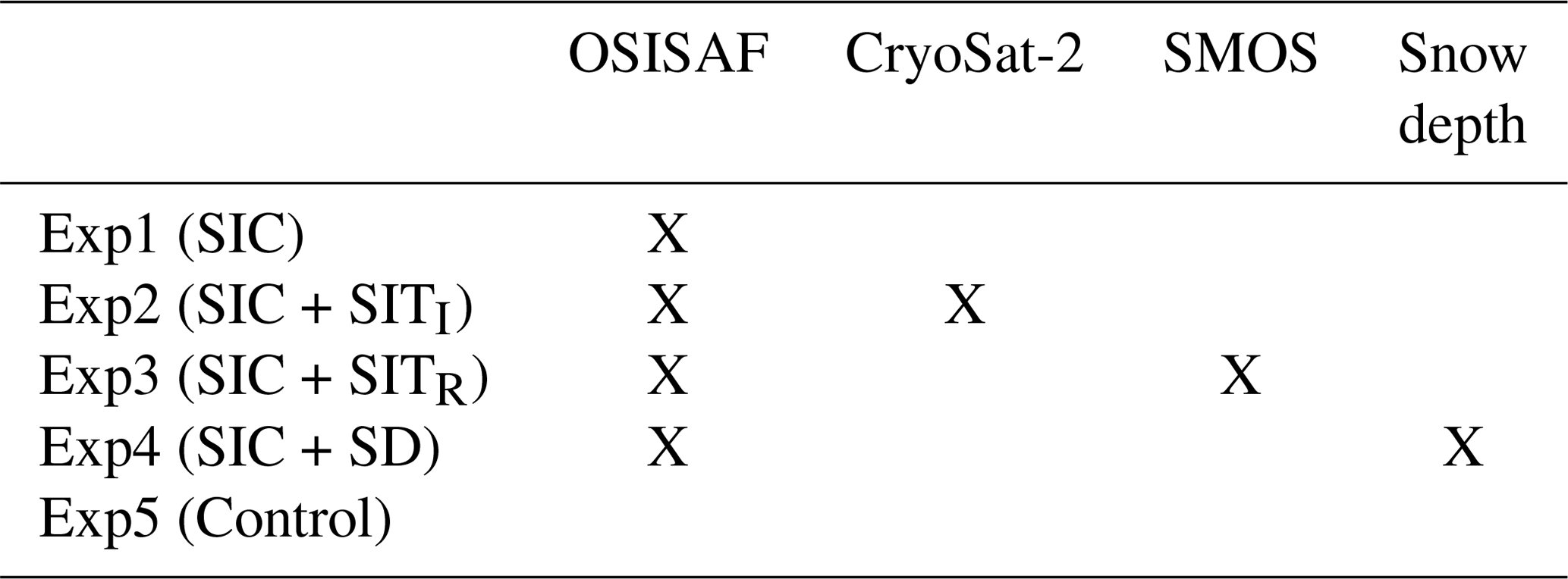
Five experiments assimilating different observations are used to investigate the effect of observations on the model. In experiment 1 only OSISAF SIC is assimilated, in experiment 2 both OSISAF SIC and CryoSat-2 SIT, in experiment 3 both OSISAF SIC and SMOS SIT, in experiment 4 OSISAF SIC and snow depth (SD) observations, and experiment 5 is a control run without assimilation. All assimilation systems are initialised after 1 year of initial assimilation on 1 January 2011 and run for 3 years. A summary of the different experiments is shown in Table 1.
Table 1Overview of the five experiments used to assess observation impact. The X marks a given observation that is assimilated in the experiment.
In this section, the output of the five ensemble experiments is compared. All results are based on the output from 2011 to 2013. As mentioned, the first year of modelling, 2010, is only used to spin-up the experiments, generating a stable and consistent ice–ocean model state.
Many of the results shown in this section will be based on the root mean squared error (RMSE). In this study, the RMSE is weighted by the observation uncertainty, σObs(i),
where N is the number of grid cells, Obs and Mod are the observations and model values, respectively. Thus, an RMSE of 1 indicates that the difference between model and observations are on average of the same order as the observation uncertainty.
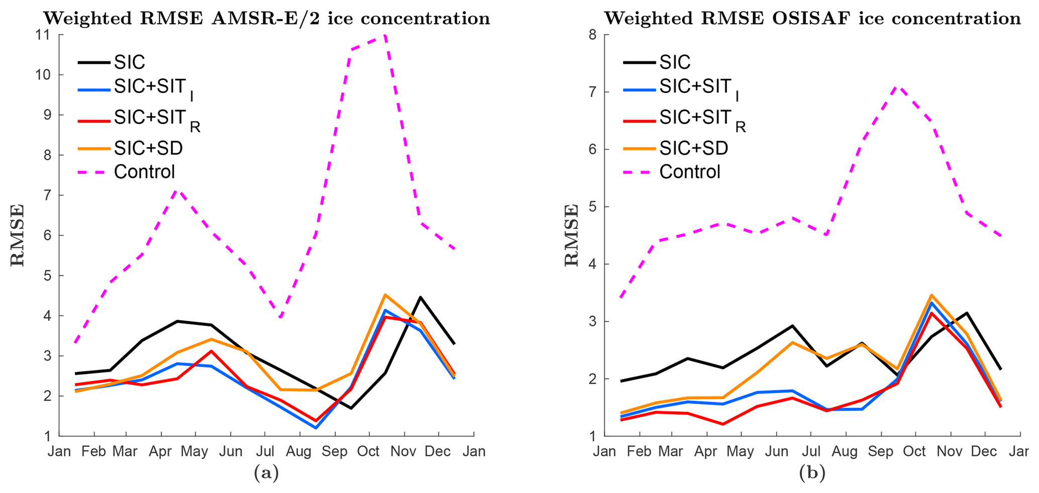
Figure 2The monthly averaged RMSE of the ensemble mean SIC over 3 years. In (a) the model is validated against AMSR-E/2 SIC observations and (b) OSISAF SIC observations. The lines represent different experiments: black is only SIC assimilation, blue is SIC and CryoSat-2 thick internal SIT assimilation, red is SIC and SMOS and thin rim SIT assimilation, yellow is SIC and snow-depth (SD) assimilation and magenta dotted is without assimilation.
5.1 Validation against concentration observations
In Fig. 2 the monthly averaged ensemble mean of the five experiments were validated against two different SIC observation products; one assimilated and one independent are plotted. In Fig. 2a the RMSE values of the ensemble mean of the modelled SIC validated with the observed AMSR-E/2 product are plotted after assimilation. All four assimilation experiments are found to be significant improvements compared to the control experiment without assimilation. Using a one-sided paired sample student t test over all 36 months of simulation, both the CryoSat-2 internal SIT and SMOS rim SIT experiments show significant improvements compared to the OSISAF SIC-only experiment on a 5 % level, but the differences are relatively small. The significance is derived using monthly data, but not yearly averaged data as in the figures. However, the snow experiment is not found to be significantly better than the OSISAF SIC-only experiment on a 5 % level: a p value of 0.23 is found. The difference between the SIT experiments and the SIC-only experiment is largest during the first half of the year, while in the second half of the year all experiments give similar results with a peak in the RMSE in October–November. This peak in RMSE is also seen in the control model, indicating a possible model problem related to the transition from the melt season to the growing season.
In Fig. 2b the monthly averaged RMSE of the model SIC ensemble mean versus the assimilated OSISAF SIC observations is plotted. The result in Fig. 2b is similar to that of (a), but the differences between the models are larger when verified against OSISAF, even though the OSISAF observations are assimilated in all experiments. This is partly related to the lower observation error in the MIZ for the OSISAF data set than for the AMSR-E/2 data set, and the OSISAF including almost an extra year of observations due to the AMSR-E/2 gap. Since the RMSE values are weighted by the observation error the differences in the MIZ are more pronounced when verified against OSISAF SIC observations. In addition, evidence that there are small differences between the two observation products is seen by different shapes on the graphs, even though the curves follow the same trends. As mentioned, the CryoSat-2 and SMOS SIT experiments are significantly better than the OSISAF SIC-only experiment. When compared to the OSISAF observations, the snow-depth assimilation experiment is also found to be significantly better than the OSISAF SIC-only experiment: there are significant differences, especially during the first half of the year. In conclusion, assimilating SIT and to some degree, snow depth has a significant effect on the SIC RMSE, and the effect is largest for the first half of the year. In the transition from melting ice to freezing ice, all four experiments give similar high RMSE values.
RMSE estimates are sensitive to individual measurements, contributing to large portions of the total RMSE; thus, a small area with large errors will obscure the overall model results. Another assimilation quality measure is hit rates, where all grid cells are given equal weight in the analysis. In our work, the hit rate is analysed by classifying the SIC in three categories: open water (concentration less than 10 %), low concentration (<50 %), and high concentration (>50 %). The hit rate is defined as the number of grid cells correctly classified. The independent AMSR-E/2 observations are used for verification. In Fig. 3a the number of grid cells correctly classified is shown; in Fig. 3b the number of grid cells with modelled ice and observed water are shown; in Fig. 3c the number of grid cells with modelled water and observed ice are shown; in Fig. 3d the number of grid cells with a wrong concentration category are shown, with high SIC classified as low SIC and vice versa. All assimilation experiments outperform the control run in terms of hit rate. The control run has a large number of false positives, indicating too much ice. Among the experiments, the variations are small in spring, autumn and winter, while summer shows significant differences. In summer all experiments have a minimum, which is related to an underprediction of sea ice and wrong classification of concentration in observations due to melt ponds on ice, which leads to an underestimation of SIC in the observations (Kern et al., 2016). In summer the CryoSat-2 assimilation has the highest number of hits, closely followed by the SMOS and snow experiments.
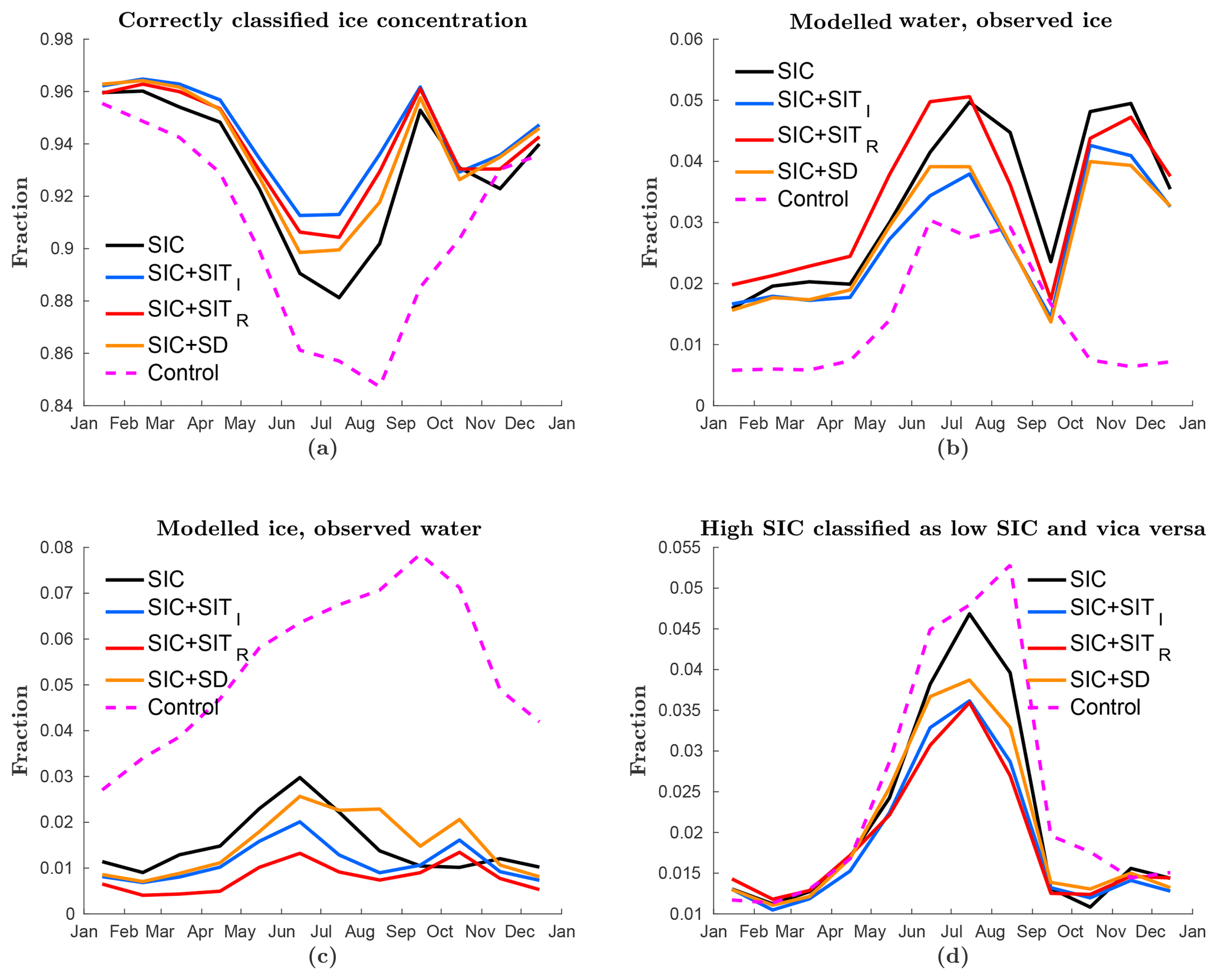
Figure 3Classification of the model result based on three classes: high-concentration ice (>50 %), low concentration ice (<50 %) or water and compared to AMSR-E/2 SIC observations. The figures show (a) the fraction of correctly classified grid cells, (b) the fraction of grid cells with modelled ice while water is observed, (c) the fraction of grid cells with modelled water while ice is observed, and (d) fraction of grid cells where the model and observations have different SIC classification. The colour coding in the figure is the same as that of Fig. 2. These panels cover all possible classifications; thus the sum of them equals one.
5.2 Total extent and volume
In Fig. 4, the total sea ice extent (Fig. 4a), the total sea-ice volume (Fig. 4b), and the total sea-ice volume overlapping the area and period covered by the CryoSat-2 internal SIT observations (fig. 4c) are shown for the five experiments. Figure 4a shows that the control experiment has a too large sea-ice extent both in summer and winter, while the assimilation experiments have a slightly too large ice extent in winter.
The total sea-ice volume shown in Fig. 4b indicates large differences between the five experiments. Snow depth assimilation generally leads to thicker ice. The model has a lower amount of snow than the observations, and due to a positive correlation, the ice thickness is also increased during the assimilation of snow depth. The increased thickness can be seen by the fact that the snow-depth experiment has about the same extent as the other experiments, but shows a significantly larger ice volume, both in summer and winter for all 3 years. Both the SMOS and CryoSat-2 ice thickness experiments lead to thinner sea ice compared to the control experiment. In particular, the SMOS assimilation model shows much thinner sea ice than the other assimilation experiments. The thin SIT observations have a very strong effect on the modelled SIT, seen by an abrupt update of sea-ice volume during assimilation in winter. A concerning effect of the assimilation experiments is the strong decrease in the Arctic sea-ice volume throughout the period of study. The sea-ice volume maximum in winter decreases for every year of assimilation; this is not seen in the control run.
In Fig. 4c the modelled sea-ice volume is compared to the sea-ice volume in the combined CryoSat-2-SMOS product. The control model is found to have too thick ice compared to the observations, while the experiments assimilating SIT are much closer to the observations, though largely biased. This can be used to explain the drastic decrease in sea-ice volume found in Fig. 4b. The model SIT is adjusting to the observations by rapidly thinning the sea ice. For the OSISAF SIC-only assimilation experiment, the volume is also slowly diverging towards the observed volume, even though SIT is not assimilated. This is likely related to a more accurate sea-ice extent that also leads to improved ice thickness in the marginal ice zone. However, the improvements are obtained at a slower pace than when assimilating SIT directly.
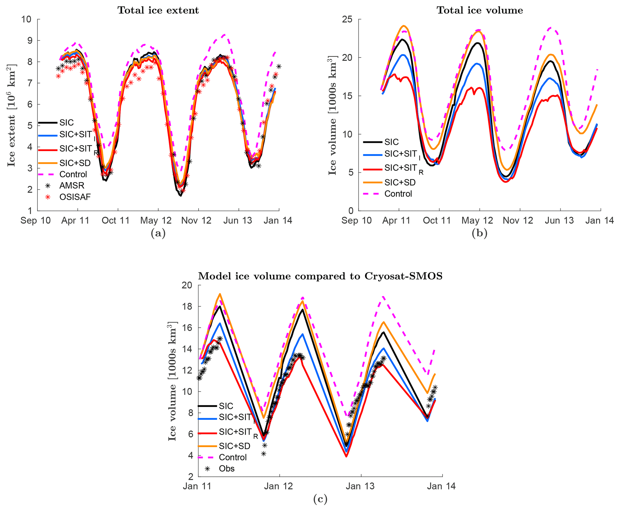
Figure 4The evolution of (a) total sea-ice extent, (b) total sea-ice volume and (c) total sea-ice volume for the area covered by the CryoSat-2-SMOS SIT observation product. The coloured lines represent the same as in Fig. 2. In (a) the black stars represent the AMSR-E/2 SIC observations and the red stars the OSISAF SIC observations. In (b) same as (a) without observations. In (c) the black stars represent the CryoSat-2-SMOS observation product. The x label is given as month and year.
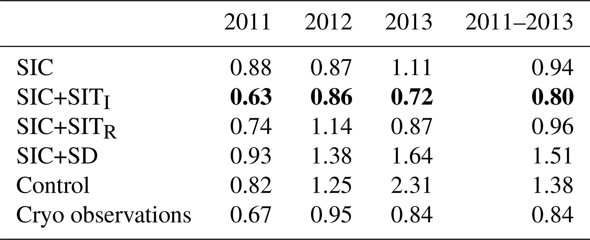
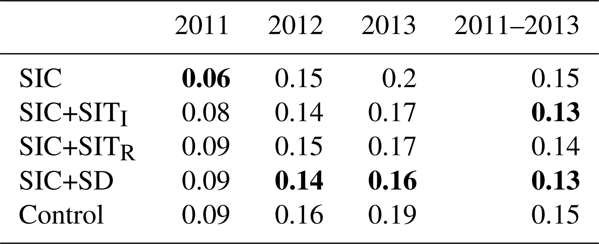
Table 2The March–April averaged RMSE values of the five experiments compared to the IceBridge aerial SIT observations. Bold values represent the model with the lowest RMSE values for that year.
5.3 Validation against thickness observations
In Fig. 5a the SIT RMSE of the ensemble mean modelled SIT is verified with the combined SMOS-CryoSat-2 SIT product. The experiment assimilating SMOS thin SIT has significantly lower RMSE values than the other three assimilation experiments. The other three experiments are more similar, all showing high RMSE values. It is found using a one-sided paired student t test that only the SMOS SIT experiments are significantly better than the SIC-only assimilation, with p values less than 5 %. Due to the high RMSE values, only small improvements are seen compared to the control run. The result is consistent with what was found for the sea-ice volume (Fig. 4c), regarding the SMOS SIT assimilation having the strongest effect on the modelled SIT. The reason for the high RMSE values is that, in general, the model has too much ice, leading to too thick ice in the MIZ. For the SMOS-CryoSat-2 SIT product, the uncertainties provided are very small, especially in the MIZ where the SMOS observations are used; thus when calculating the RMSE these values have a huge effect on the result. Thus, it is also reasonable that the assimilation system for these MIZ-thickness observations also gives the lowest RMSE values. For the other assimilation systems, the ice extent is updated in the MIZ, but the thickness reduction takes longer because it has to evolve over time.
As for the SIC observations, the RMSE values are biased by locations showing large differences. Particularly for thickness which is not bounded upwards, a few grid cells in the MIZ can contribute to a large total RMSE. As for concentration, an alternative measure is one in which correctly classified model thickness hit rates are used. The model is separated into four thickness categories: less than 0.5 m, between 0.5 and 1.5 m, between 1.5 and 3 m, and above 3 m. In Fig. 6a the number of correctly classified ice thicknesses grid cells is plotted for each experiment. The figure shows that the CryoSat-2 internal SIT experiment is the model which has the highest number of correctly classified grid cells. The other experiments are more similar, except in spring where the SMOS rim SIT assimilation is equally good as the CryoSat-2 internal SIT assimilation, and both are much better than the other three. In spring the SIC-only and snow-depth assimilations are not improved compared to the control case. In general, the model shows too much ice. This can be seen by a large number of grid cells having too thick ice in the control model (Fig. 6b). This is a combination of the sea-ice extent being too large and the ice being too thick. By assimilating the observations, the ice volume is reduced, not only for the SIT assimilations, but also for the snow-depth and SIC-only assimilations, but to a lower degree for the latter. This is an effect of a lower sea-ice extent (Fig. 4a). In Fig. 6c the number of grid cells with too thin ice compared to the observations is shown. It was found that this is a big problem in early winter for all experiments but reduces during winter for all experiments except the SMOS experiment. During SMOS assimilation, only thin ice is assimilated, which might lead to a bias towards the thinner ice, causing a relatively high number of grid cells with too thin ice.
As an example, in Fig. 7 the absolute differences between the experiments and the combined CryoSat-2 SMOS ice thickness observations are plotted for 1 April 2011. Figure 7 is consistent with Fig. 6a, showing that the CryoSat-2 experiment has the smallest differences compared to the observations in the internal Arctic, affecting a large area; however, large differences can be seen in MIZ. While for the SMOS rim SIT assimilation the effect is the opposite, with a large impact in the MIZ and small impact in the ice interior. This shows that assimilating SIT is important both in the interior and in the MIZ.
In addition to the satellite observations, the independent airborne IceBridge data set is used for verification of the modelled SIT (Kurtz et al., 2013, 2014a). This data set has low temporal and spatial distributions, but is believed to have higher accuracy and much higher spatial and temporal resolutions. All observations occurring in March and April are gathered as a yearly averaged observation as a function of space. These yearly observations are then compared to modelled SIT averaged over the same period for the observed IceBridge locations. Since the IceBridge resolution is much higher than that of the model, all IceBridge observations within one model grid cell are averaged and used for verification. The average is done by a weighted mean based on the observation uncertainty. The validation results are shown in Table 2. On average, the CryoSat-2 SIT experiment has the best SIT estimation as compared to IceBridge. Both the SMOS and the CryoSat-2 SIT experiments give on average thinner SIT than the IceBridge observations, which are consistent with the findings of Chen et al. (2017). The last line in the table shows the RMSE between the CryoSat-2 observations and the IceBridge observations and the results show that the error is comparable to the model errors.
For all 3 years, the CryoSat-2 assimilation has lower RMSE values than the CryoSat-2 observations, indicating a well-balanced assimilation, with appropriate observation error and ensemble spread. It should also be mentioned that the CryoSat-2 observations have less spatial coverage than the model and not all IceBridge observations are covered; thus the number of useful observations for the CryoSat-2 RMSE calculation are smaller than for the validation of the experiments.
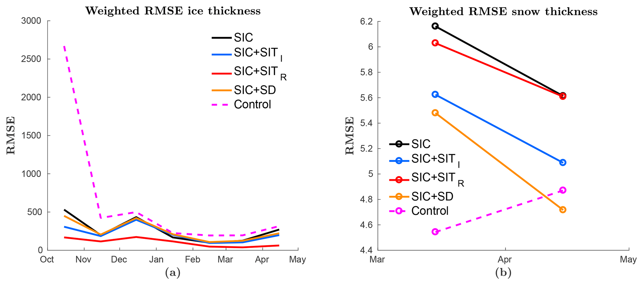
Figure 5RMSE of monthly averaged model SIT and snow depth averaged over all ensemble members for the years 2011–2013 calculated against the (a) combined SMOS-CryoSat-2 SIT product and (b) observed snow-depth product. These are observations also used for assimilation. The colour coding is as in Fig. 2.
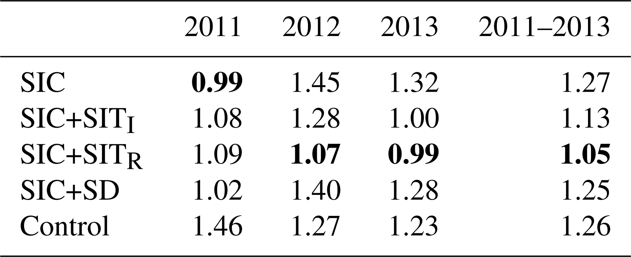
Another independent data set of SIT observations complementing the IceBridge observations by a temporal resolution spanning the entire year is the IMB buoy data set. The result of model validation with the IMB product is shown in Table 3. For these observations, a slightly different method than that applied for IceBridge is performed. This is because IceBridge temporarily only covered March–April, while the IMB data span the entire year. The buoy observations are converted to daily averages on the model grid. From these values, the RMSE is calculated on the 7-day ensemble mean and averaged for each year. Since SIT is a relatively slow varying variable, for each 7-day output, observations from ±3 days are used to increase the number of observations. The IMB observations do not include an uncertainty estimation; hence the RMSE is not normalised as was the case for other RMSE estimates in this work. The results show that over the 3 study years, the SMOS internal SIT assimilation system has the lowest RMSE values, followed by the CryoSat-2 internal SIT assimilation. The other three show similar results, again indicating a positive impact of assimilating ice thickness in the model.
Table 3The yearly averaged RMSE values of the five experiments compared to the IMB SIT buoy observations. Bold values represent the model with the lowest RMSE values for that year. No uncertainties are used to normalise the RMSE values.
5.4 Validation against snow observations
In Fig. 5b the RMSE of monthly averaged modelled snow depth is plotted over all ensembles validated against the observed satellite snow depth (Rostosky et al., 2018) used for assimilation. The control experiment is found to have the lowest RMSE values. This is most likely an effect of sea-ice extent being different to the assimilation experiments, rather than the assimilation declining the accuracy of the modelled snow depth. In addition, the control experiment has an increasing RMSE during the period, while the assimilation experiments show the effect of assimilation by decreasing the RMSE. For the assimilation experiments, the snow experiment has the lowest RMSE values followed by the CryoSat-2 experiment, indicating that the thick ice observations have a correlation effect on the snow depth. These two observation products also cover a similar area of the Arctic Ocean.
A verification of the modelled snow depth using the independent IceBridge data set is given in Table 4. The same method as for the SIT in Table 2 was used, where March–April model values are compared to the IceBridge observations and averaged. It is found that none of the experiments are particularly better than any of others when verified against IceBridge snow-depth observations. It is seen that, within one grid cell, there are huge variations in the IceBridge snow observations. Such variations cannot be provided with a coarse-resolution model. Hence, even though IceBridge is used to “tune” the snow observations (Rostosky et al., 2018), large RMSE values are estimated for the experiment assimilating snow depth. In addition, the snow component used in our coupled system is likely too simple, having only one snow layer, which may affect the snow cover accuracy. It is also important to mention that the snow observations are in an early development stage and might have larger uncertainties than those used in this study.
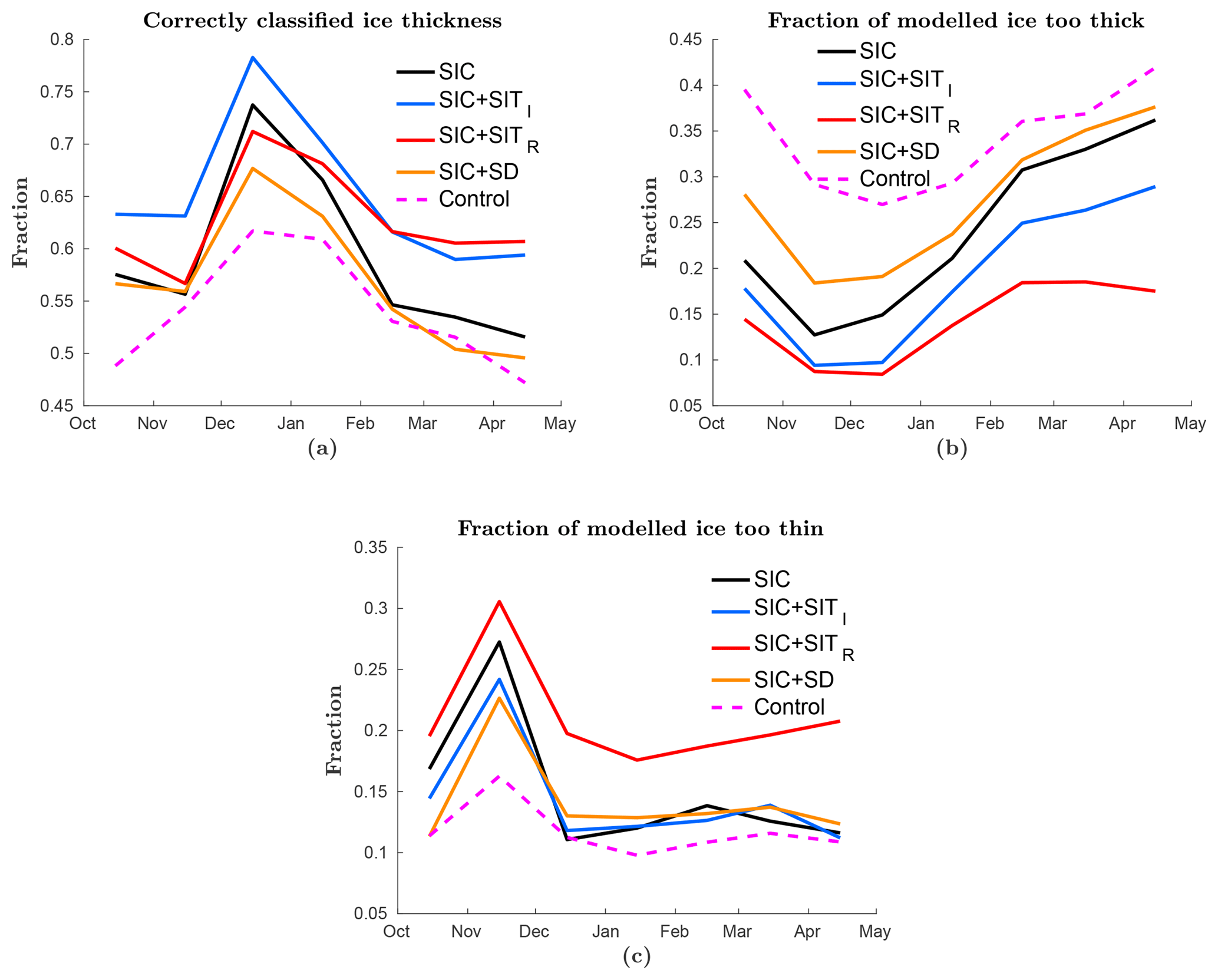
Figure 6The monthly mean SIT averaged over all ensemble members is classified into four thickness categories and compared to the CryoSat-2-SMOS SIT observation product. The fraction of grid cells are shown with (a) correctly classified thickness category, (b) too thick ice, and (c) too thin ice. As in Fig. 2 the coloured lines represent different experiments.
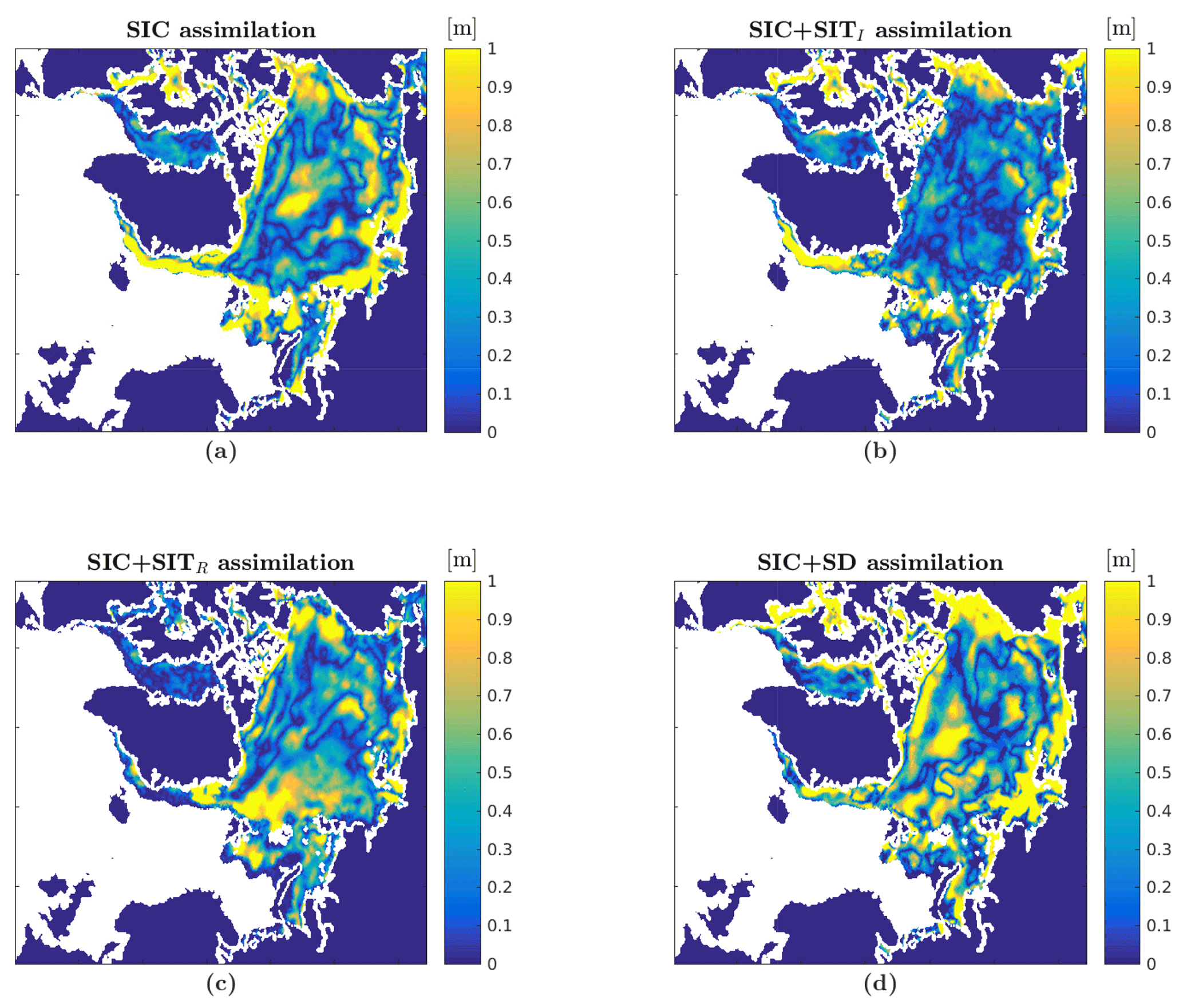
Figure 7Absolute differences between the experiments and the combined SMOS-CryoSat-2 observation product are given on 1 April 2011. The experiments are assimilating (a) OSISAF SIC, (b) OSISAF SIC and CryoSat-2 SIT, (c) OSISAF SIC and SMOS SIT and (d) OSISAF SIC and snow depth.
Table 4The March–April-mean RMSE of the ensemble-mean snow depth averaged over all grid cells. The five experiments and the snow-depth satellite observations are compared to the IceBridge airborne snow-depth observations. Bold values represent the model with the lowest RMSE values for that year.

NA – not available
Additional model verification is performed with the independent IMB buoy snow-depth observations. The method of validation is performed in a similar manner as for SIT validation with IMB buoy data: the results are shown in Table 5. As the IMB data do not include an uncertainty these RMSE values are not normalised; thus they are significantly lower than the error estimates from the ice bridge validation in Table 4. From the table it is clear that the differences between the assimilation systems are small. The assimilation systems for snow depth and CryoSat-2 internal SIT are slightly better than the others, but the differences are too small to obtain conclusions.
Table 5The yearly averaged RMSE values of the five experiments compared to the IMB snow-depth buoy observations. Bold values represent the model with the lowest RMSE values for that year. No uncertainties are used to normalise the RMSE values.
5.5 One week forecasts
Figure 8 shows the RMSE of the monthly averaged modelled SIC over all ensemble members before assimilation validated against the AMSR-E/2 and OSISAF SIC observations. Since the assimilation time step is 7 days, this gives the accuracy of a 7-day forecast. The comparison against AMSR-E/2 SIC observations (Fig. 8a) shows that the differences between the experiments are small, and the differences are similar to those found after assimilation (Fig. 2a). In general, the system with the most accurate initial state also gives the most accurate forecasts. Thus, the CryoSat-2 and SMOS SIT assimilation experiments have a better 7-day forecast from January to June than SIC only, and snow-depth assimilation shows improvements from January to April. Using the OSISAF SIC observations (Fig. 8b) gave the same result as found for AMSR-E/2: the best initial states also provide the best forecast, indicating that the sea ice does not change much overall in a week. The same experiments were also done for ice thickness and snow depth and similar results were encountered. A reason for the small differences between the different experiments is the coarse model resolution. Large-scale variations as seen by a 20 km model are not expected within a week.
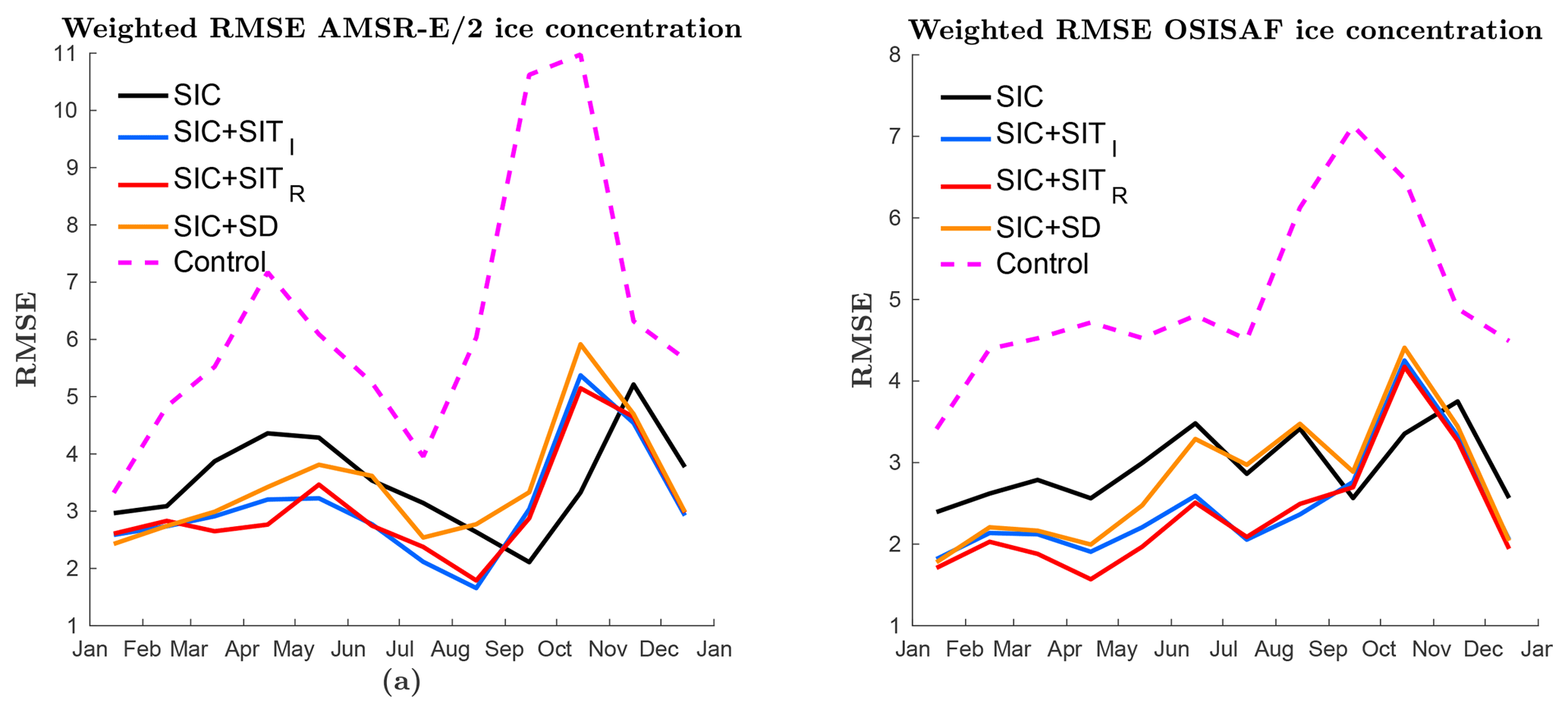
Figure 8RMSE of monthly averaged (over 3 years) ensemble mean of 7-day forecast SIC validated against (a) AMSR-E/2 SIC observations and (b) OSISAF SIC observations.
In the previous section, it was found that our coarse-resolution model only exhibits small changes during a 1 week forecast. Thus, a more interesting forecast would be one of seasonal length. A 5-month forecast of the September sea-ice extent is performed. This is done by running each of the experiments from mid-April to mid-September each year without assimilation and validating them against the OSISAF SIC observations. The actual start date varied slightly from year to year because of the 7-day assimilation cycle, but the start date was the same for all experiments. In Fig. 9a, the RMSEs of three 5-month forecasts are shown sequentially, and a monthly averaged RMSE over the 3 years is shown in Fig. 9b. The figures show that the experiments have very similar seasonal forecasts, with some differences in late summer. In general, the model error is gradually increasing towards the level of the control run, and in summer they have similar error levels. In August–September the experiments assimilating thickness and concentration seem to be improved compared to those without assimilation and assimilating snow-depth observations. All experiments show an increased RMSE in 2013: this is related to a too low sea-ice extent. The low sea-ice extent is caused by weaker modelled ice growth compared to observations in the first months of 2013.
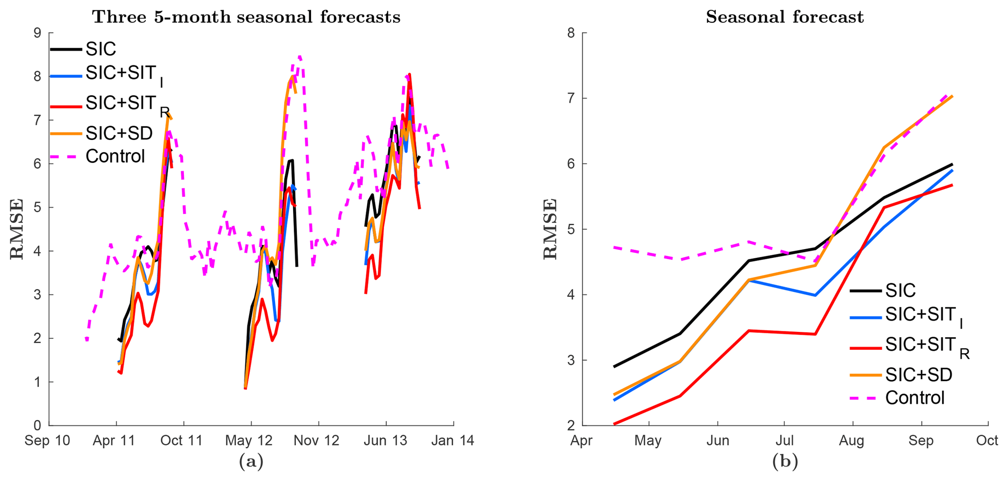
Figure 9Seasonal forecast of summer sea-ice extent. Each forecast started at the beginning of April every year. The figures show the RMSE of the ensemble mean SIC averaged over 3 years and verified against the assimilated OSISAF SIC. The coloured lines represent the same as in Fig. 2. (a) Full period and (b) monthly averaged values.
The seasonal forecast is compared to a climatological seasonal forecast in Fig. 10. This provides an estimate of the expected sea-ice forecast accuracy. The climatological experiment is done by running the model with averaged atmospheric forcing data over the years from 2000 to 2014. The result shows that the forecast skill of the model is rapidly decreasing and that a correct atmospheric forecast is very important for an accurate sea-ice forecast. Still, skills are evident on much longer timescales that can be obtained with numerical weather prediction models.
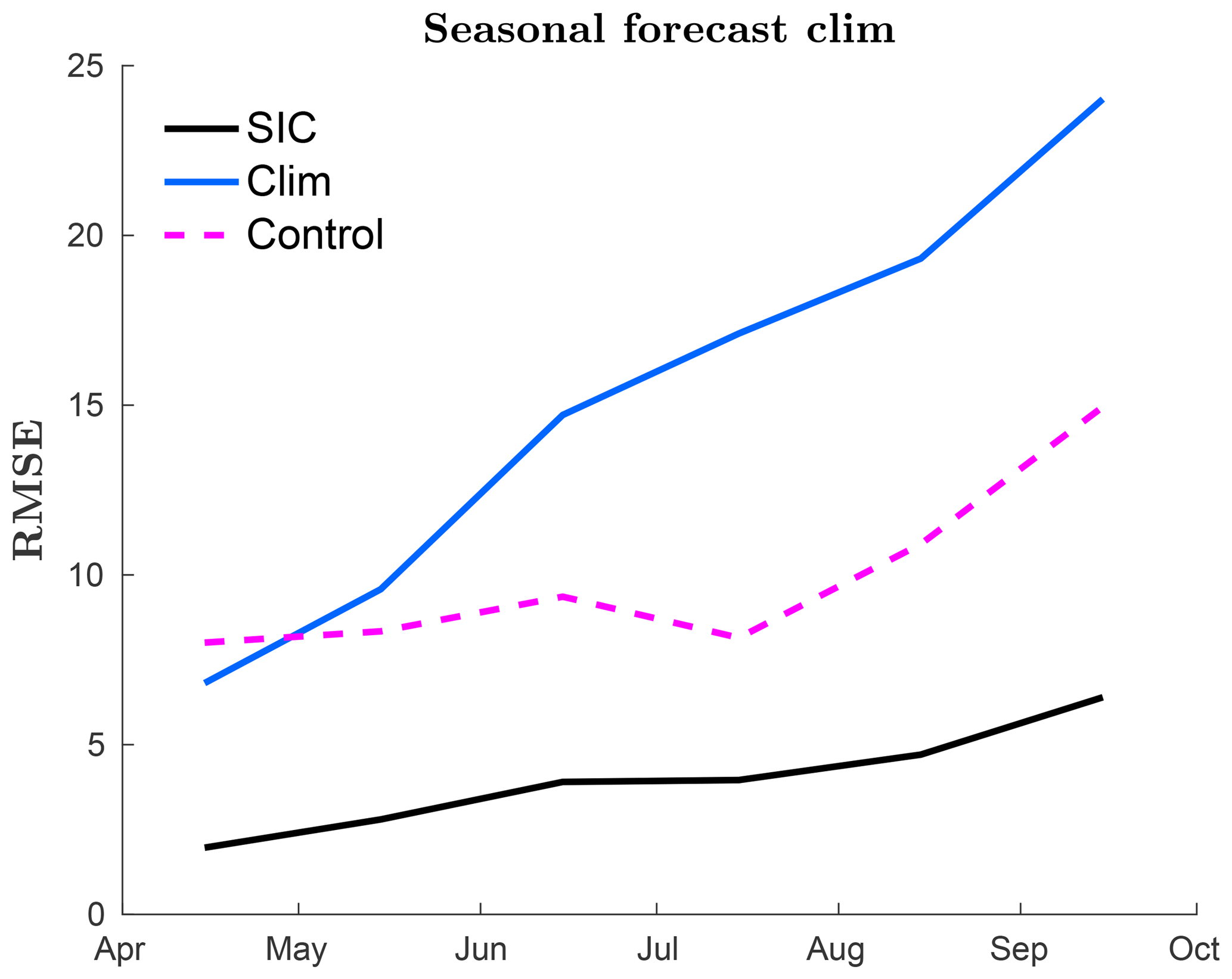
Figure 10Seasonal forecast of summer sea-ice extent, both with climatological forcing and reanalysed forcing. Each forecast started at the beginning of April every year. The figure describes monthly averaged RMSE SIC averaged over all ensemble members. The blue line represents a forecast using a climatological forcing made from atmospheric data over 2000–2014 with assimilation, the black line using reanalysed atmospheric forcing and assimilation, and the dotted magenta line use reanalysed forcing only.
Significant differences in modelled SIC after assimilation was found, especially in the first half of the year. The SMOS and CryoSat-2 SIT assimilations gave the lowest RMSE values, which are significantly better than when assimilating OSISAF SIC-only. The snow-depth experiment showed improvements during the first half of the year compared to the experiment assimilating OSISAF SIC observations only. In addition, assimilating SIT and snow depth lead to an improved model of SIC in summer, where the CryoSat-2 internal SIT assimilation gave the highest number of correctly classified grid cells, closely followed by the SMOS rim SIT and snow-depth assimilations. The reason for these differences in summer is that the pace at which the ocean becomes ice-free is dependent on the ice thickness and the snow depth. In the second half of the year, autumn and early winter, all our experiments gave similar results. These similarities seem to be a consequence of the transition from melt season to growing season not being well represented in the model. The observed transition is faster than the modelled, leading to an extended period with more open water in the model than in the observations.
In the control model without assimilation, the ice extent both in summer and winter was found to be larger than observed. However, with assimilation, the experiments are closer to the observed extent, even though a slight overestimation of extent in winter was found for the first 2 years. The sea-ice extent overestimation in winter is a result of a lower effect of SIC assimilation in winter due to lower ensemble spread. When the ensemble spread is low the EnKF assimilation result is closer to the model values, because the estimated model errors become small.
It is found that originally the sea-ice volume is too large compared to the observations, and over the 3 years, the sea-ice volume in the assimilation experiments are gradually decreasing towards the observed values in the SMOS-CryoSat-2 SIT product. The effect is much stronger for the SMOS rim SIT assimilation, indicating that a large portion of the original sea-ice volume overestimation is located in the MIZ. This is a consequence of too much ice in the control model, causing the observed MIZ to be located deeper in the Arctic compared to the model, as noted by Fritzner et al. (2018).
In the verification of modelled SIT (Fig. 5a), the SMOS rim SIT assimilation was found to give the lowest RMSE values, while the CryoSat-2 internal SIT assimilation had the largest amount of correctly classified thickness grid cells. This is as expected since, even though the CryoSat-2 observations cover a larger area, they are 30-day averaged observations with much larger uncertainties than the SMOS observations. In addition, the non-updated grid cells in the MIZ lead to larger RMSE values than non-updated grid cells in the internal Arctic, where the model, in general, is more accurate and less sensitive to changes. When verified by IceBridge observations, which only cover the central Arctic, the CryoSat-2 SIT assimilation experiment was found to give the lowest SIT RMSE values. The CryoSat-2 SIT observations are in general thinner than the SIT values for the SIC-only experiment. In comparison with the IceBridge observations, the CryoSat-2 SIT is biased low, which was also found by Chen et al. (2017). When assimilating snow depth, it was found that snow-depth observations, in general, were thicker than those modelled, resulting in increased snow depth during assimilation. Due to the correlation nature of the EnKF, a positive correlation between snow depth and SIT resulted in increased SIT in the snow-depth assimilation experiment compared to the other assimilation experiments.
Validating our experiments with snow observations proved the control run to have the lowest RMSE values. This can be an effect of different sea-ice extents in the control run than in the assimilation experiments. For the control model, the ice extent is too large, thus collecting more snow on the ice than the assimilation experiments. When the ice concentration is reduced during assimilation, the accumulated snow is also removed, which can result in the removal of too much snow if the ice extent is less than it should be. A verification of the impact of assimilation on the snow depth is that the RMSE is decreasing throughout the observation period for the assimilation experiments, while for the control run the RMSE is increasing. Between the assimilation experiments, the snow-depth assimilation was found to give the lowest snow-depth RMSE values, which is not unexpected since the same data set is used for assimilation and verification. More interestingly the CryoSat-2 internal SIT experiment has significantly lower RMSE values than the SMOS rim SIT and OSISAF SIC-only assimilations, indicating a close correlation between SIT and snow depth. A curiosity here is that the SIT assimilation has a positive effect on the snow depth, while it was found previously that the snow-depth assimilation had a negative effect on the SIT. This is likely an effect of more SIT observations than snow-depth observations, and SIT is assimilated throughout the whole winter. It could be the case that the correlation relationship between snow-depth and SIT changes throughout the winter. This results in a better snow-depth estimate for SIT assimilation, while for snow-depth assimilation the assimilation period is limited to March–April. In addition, when a parameter is only assimilated during two months of the year, the model error is larger when the assimilation period starts; thus the assimilation update has a large effect both on snow depth and SIT. An indication of the relation between SIT and snow depth is also seen by lower snow-depth RMSE values for the SMOS rim SIT assimilation than the OSISAF SIC-only assimilation. Since the SMOS system covers a much smaller area and has less overlap with the snow data set than the CryoSat-2 internal SIT, the effect of assimilation on the modelled snow is smaller.
When validating our experiments with the IceBridge snow-depth observations, none of the experiments showed any improvement compared to the others. This can be related to an underestimated uncertainty in the snow observations or that the snow representation in the model is too simplistic, only utilising a single layer. Another problem is local variations: the coupled model is coarse with a resolution of 20 km, but, as can be seen from the IceBridge observations, the snow depths have large spatial variations in this range. This causes high RMSE values, both compared to satellite observations (on the model grid) and the modelled snow-depth values. In addition only 4 months of snow-depth observations were available for assimilation during the 3 years.
For sea ice, the model drift is in general small, the model system with the best initial state provides the best short-term forecast. The main parameters analysed in this study, snow depth, SIT and SIC, all vary on timescales longer than 1 week for the spatial resolution in our model. Thus, the correlation between day 1 and day 7 is too strong. As also shown by Chen et al. (2017), the sea-ice drift is low.
Several 5-month seasonal forecasts of the September sea-ice extent showed small differences between the assimilation experiments. All experiments showed a steady increase in RMSE with time. This is likely caused by the model overgrowth of ice. The seasonal forecasts showed that after 3–4 months the RMSE values were found to be of the same order as those in the control run. Thus, assimilation gives at least an improvement over 3–4 months, and the September result suggests that with the assimilation of SIC and SIT there are improvements in the Arctic sea-ice extent compared to the control run on even longer timescales. This was not seen for the snow depth experiment. The seasonal forecast was compared to a climatological run, and it was found that without accurate forcing the forecast degenerates fast.
In this work, four different observation products have been used for assimilation. The different products differ widely in both temporal and spatial coverage in addition to accuracy. There is no doubt that it is preferable to have as much coverage and as accurate observations as possible. Where a realistic observation error is a necessity for the assimilation, without a realistic observation error, the observation is not useful. For example, the CryoSat-2 product does not provide an observation error and a uniform error was chosen, which will lead to some observations being given too much weight and others too little. In this study, the spatial resolution of the observations is not a problem, because the model resolution is coarse, but in the future, when the model resolution increases, there will be an increasing demand for high-resolution SIT observations. Both SIT products are only available in winter, and temporal coverage of the snow-depth observations are limited to 4 months of a 3-year experiment. Thus, for these products to be even more useful, there is a strong need for increased seasonal coverage, especially in summer when the Arctic sea-ice extent is at a minimum and there is ship traffic there. Observations can then help to improve the models, thereby helping to plan operations and decrease the risks. In addition, because there are few snow observations available for assimilation, there are large unknown aspects regarding the assimilation effect. Finally, it should be remembered that the model itself has in general too much ice and that the forcing is known to contain biases and errors (Jakobson et al., 2012).
In conclusion, we have found that assimilation of more observation types than SIC into coupled sea-ice–ocean models can lead to significant model improvements. We show that the assimilation of SIT, in particular, leads to improvements in modelled SIC, SIT and snow depth for long-term model improvement. There is clear evidence that assimilation of SIT gives a better representation of the full ice state, and we recommend that they are assimilated into models when available. Even though SIT seems to be an important variable for improving sea-ice modelling, it still has several limitations in terms of spatial and temporal resolution and realistic observation errors. It is important to emphasise that assimilation of SIC is vital to the assimilation update: these observations give important information with full Arctic coverage on where the ice is located. In addition, the fractional ice in the MIZ is important for the forecast in terms of how the short-term changes in the sea-ice will look, and also an indication of the thickness.
Assimilation of snow depth was found to have a weaker effect on the model than assimilating SIT, but improvements to modelled SIC and modelled snow depth were found. In addition, we found a strong correlation between SIT and snow depth, which should be analysed further when more observations from other months become available. The low efficiency of snow-depth observations can be related to the low model resolution. The IceBridge observations show large snow-depth variations within a model grid cell. It is also important to keep in mind that the snow-depth observations are in an early development stage, and the uncertainty estimations might not be correct. Possibly inaccurate observations or a wrong uncertainty estimation can have a huge impact on the assimilation result. Due to the small temporal coverage in our study more investigation has to be done on the effect of assimilating snow-depth observations.
As mentioned, the assimilation of SIT leads to an improved model, which leads to improved short-term forecasts over time, because the initial states are better represented. For the seasonal forecast, we found that the model improvements due to assimilating observations have a memory of at least 3–4 months, and possibly even longer. Assimilating SIC and SIT showed improvements of the September ice forecasts compared to assimilating snow depth and no assimilation.
Comparing the two SIT products, SMOS thin SIT and CryoSat-2 thick SIT, we see that, in general, the CryoSat-2 observations give the best long-term model improvement, but especially for decreased RMSE values in summer. It is expected that the SMOS observation assimilation should be better for the short-term forecast, but we were not able to provide any results on this. This could be an effect of the model resolution being too low. With 20 km resolution the ice state does not change much over a week of simulation.
The model output used for the analysis in this study is published in the NIRD Research Data Archive, https://doi.org/10.11582/2019.00005 (Fritzner, 2019).
SF sat up the assimilation system, ran all the experiments and did the analysis. RG provided ideas and feedback on the study. KHC assisted with running the ROMS model and gave helpful feedback on the study. PR made the snow observations used for assimilation. KW assisted in running the CICE model and provided feedback on the study. SF wrote the manuscript with contributions from all the co-authors.
The authors declare that they have no conflict of interest.
We would like to thank Pavel Sakov for help in using and implementing the EnKF-c code and for helpful discussions regarding the EnKF. We thank the EUMETSAT OSISAF centre and the NASA National Snow and Ice Data Center for providing the sea-ice concentration data, and the Integrated Climate Data Center at the University of Hamburg for the SMOS ice thickness observations. We would like to thank the NASA National Snow and Ice Data Center for providing the Cryosat sea-ice thickness observation and the IceBridge snow and sea-ice thickness observations.
This work was funded through the Center for Integrated Remote sensing and
Forecast for Arctic Operations through the Norwegian Research Council grant
no. 237906. Rostosky was supported by the Transregional Collaborative
Research Center (TR 172) ArctiC Amplification: Climate Relevant Atmospheric
and SurfaCe Processes, and Feedback Mechanisms (AC)3, which is funded by
the German Research Foundation (DFG). Two supercomputers provided by the
Norwegian Metacenter for Computational Science (NOTUR) were used for the
computational work. The Vilje computer at the Norwegian University of Science
and Technology was used with the project and the Stallo computer at the
University of Tromø, both of which are under project
NN9348K.
Edited by: John Yackel
Reviewed by: two anonymous referees
Allard, R. A., Farrell, S. L., Hebert, D. A., Johnston, W. F., Li, L., Kurtz, N. T., Phelps, M. W., Posey, P. G., Tilling, R., Ridout, A., and Wallcraft, A. J.: Utilizing CryoSat-2 sea ice thickness to initialize a coupled ice-ocean modeling system, Adv. Space Res., 62, 1265–1280, https://doi.org/10.1016/j.asr.2017.12.030, 2018. a
Andersen, S., Tonboe, R., Kern, S., and Schyberg, H.: Improved retrieval of sea ice total concentration from spaceborne passive microwave observations using Numerical Weather Prediction model fields: An intercomparison of nine algorithms, Remote Sens. Environ., 104, 374–392, 2006. a
Bell, M., Barciela, R., Hines, A., Martin, M., McCulloch, M., and Storkey, D.: The forecasting ocean assimilation model (FOAM) system, in: Elsevier oceanography series, Elsevier, vol. 69, 197–202, 2003. a
Blockley, E. W. and Peterson, K. A.: Improving Met Office seasonal predictions of Arctic sea ice using assimilation of CryoSat-2 thickness, The Cryosphere, 12, 3419–3438, https://doi.org/10.5194/tc-12-3419-2018, 2018. a
Burgers, G., van Leeuwen, P., and Evensen, G.: Analysis Scheme in the Ensemble Kalman Filter, Mon. Weather Rev., 126, 1719–1791, https://doi.org/10.1175/1520-0493(1998)126<1719:ASITEK>2.0.CO;2, 1998. a
Caya, A., Buehner, M., and Carrieres, T.: Analysis and Forecasting of Sea Ice Conditions with Three-Dimensional Variational Data Assimilation and a Coupled Ice-Ocean Model, J. Atmos. Ocean. Tech., 27, 353–369, https://doi.org/10.1175/2009JTECHO701.1, 2010. a
Chen, Z., Liu, J., Song, M., Yang, Q., and Xu, S.: Impacts of Assimilating Satellite Sea Ice Concentration and Thickness on Arctic Sea Ice Prediction in the NCEP Climate Forecast System, J. Climate, 30, 8429–8446, 2017. a, b, c, d, e
Comiso, J., Cavalieri, D., and Markus, T.: Sea Ice Concentration, Ice Temperature, and Snow Depth Using AMSR-E Data, IEEE T. Geosci. Remote., 41, 243–252, https://doi.org/10.1109/TGRS.2002.808317, 2003. a
Dee, D. P., Uppala, S. M., Simmons, A. J., Berrisford, P., Poli, P., Kobayashi, S., Andrae, U., Balmaseda, M. A., Balsamo, G., Bauer, P., Bechtold, P., Beljaars, A. C. M., van de Berg, L., Bidlot, J., Bormann, N., Delsol, C., Dragani, R., Fuentes, M., Geer, A. J., Haimberger, L., Healy, S. B., Hersbach, H., Hólm, E. V., Isaksen, L., Kållberg, P., Köhler, M., Matricardi, M., McNally, A. P., Monge-Sanz, B. M., Morcrette, J.-J., Park, B.-K., Peubey, C., de Rosnay, P., Tavolato, C., Thépaut, J.-N., and Vitart, F.: The ERA-Interim reanalysis: configuration and performance of the data assimilation system, Q. J. Roy. Meteor. Soc., 137, 553–597, https://doi.org/10.1002/qj.828, 2011. a
Donlon, C. J., Martin, M., Stark, J., Roberts-Jones, J., Fiedler, E., and Wimmer, W.: The operational sea surface temperature and sea ice analysis (OSTIA) system, Remote Sens. Environ., 116, 140–158, 2012. a
Eicken, H.: Ocean science: Arctic sea ice needs better forecasts, Nature, 497, 431–433, 2013. a
Evensen, G.: Sequential data assimilation with a nonlinear quasi-geostrophic model using Monte Carlo methods to forecast error statistics, J. Geophys. Res., 99, 10143–10162, https://doi.org/10.1029/94JC00572, 1994. a, b
Evensen, G.: The Ensemble Kalman Filter: Theoretical Formulation and Practical Implementation, Ocean Dynam., 53, 343–367, https://doi.org/10.1007/s10236-003-0036-9, 2003. a, b, c
Evensen, G.: The Ensemble Kalman Filter for Combined State and Parameter Estimation, IEEE Contr. Syst. Mag., 29, 83–104, https://doi.org/10.1109/MCS.2009.932223, 2009. a
Flato, G. M. and Hibler, W. D.: Ridging and strength in modeling the thickness distribution of Arctic sea ice, J. Geophys. Res.-Oceans, 100, 18611–18626, 1995. a, b
Forsberg, R. and Skourup, H.: Arctic Ocean gravity, geoid and sea-ice freeboard heights from ICESat and GRACE, Geophys. Res. Lett., 32, L21502, https://doi.org/10.1029/2005GL023711, 2005. a
Fritzner, S.: Model output, Article: Impact of assimilating sea ice concentration, sea ice thickness and snow depth in a coupled ocean-sea ice modeling system [Data set], Norstore, https://doi.org/10.11582/2019.00005, 2019. a
Fritzner, S., Graversen, R., Wang, K., and Christensen, K.: Comparison between a multi-variate nudging method and the ensemble Kalman filter for sea-ice data assimilation, J. Glaciol., 64, 387–396, https://doi.org/10.1017/jog.2018.33, 2018. a, b
Gaspari, G. and Cohn, S. E.: Construction of correlation functions in two and three dimensions, Q. J. Roy. Meteor. Soc., 125, 723–757, https://doi.org/10.1002/qj.49712555417, 1999. a
Houtekamer, P. L. and Zhang, F.: Review of the Ensemble Kalman Filter for Atmospheric Data Assimilation, Mon. Weather Rev., 144, 4489–4532, https://doi.org/10.1175/MWR-D-15-0440.1, 2016. a
Hunke, E. and Dukowicz, J.: An elastic-viscous-plastic model for sea ice dynamics, J. Phys. Oceanogr., 27, 1849–1867, 1997. a
Hunke, E., Lipscomb, W., Turner, A., Jeffery, N., and Elliott, S.: CICE: the Los Alamos sea Ice Model Documentation and Software User's Manual Version 5.1, Los Alamos National Laboratory, 2015a. a, b
Hunke, E., Lipscomb, W., Turner, A., Jeffery, N., and Elliott, S.: CICE: the Los Alamos Sea Ice Model Documentation and Software User's Manual, 5.1, 2015b. a
Jakobson, E., Vihma, T., Palo, T., Jakobson, L., Keernik, H., and Jaagus, J.: Validation of atmospheric reanalyses over the central Arctic Ocean, Geophys. Res. Lett., 39, L10802, https://doi.org/10.1029/2012GL051591, 2012. a
Jazwinski, A.: Stochastic processes and filtering theory, Academic, Sand Diego, California, 1970. a
Kaleschke, L., Tian-Kunze, X., Heygster, G., Patilea, C., Hendricks, S., Ricker, R., Tonboe, R., Mäkynen, M., Bertino, L., and Xie, J.: SMOS+SeaIce Final Report, ESA Support To Science Element (STSE) Contract No.: 4000112022/14/I-AM, version: August 28, Univ. Hamburg, Institute of Oceanography, 2017. a
Kern, S., Rösel, A., Pedersen, L. T., Ivanova, N., Saldo, R., and Tonboe, R. T.: The impact of melt ponds on summertime microwave brightness temperatures and sea-ice concentrations, The Cryosphere, 10, 2217–2239, https://doi.org/10.5194/tc-10-2217-2016, 2016. a
Kristensen, N., Debernard, J., Maartensson, S., Wans, K., and Hedstrom, K.: metno/metroms, https://doi.org/10.5281/zenodo.1046114, 2017. a, b
Kurtz, N. and Harbeck, J.: CryoSat-2 Level-4 Sea Ice Elevation, Freeboard, and Thickness, Version 1, Boulder, Colorado USA. NASA National Snow and Ice Data Center Distributed Active Archive Center, https://doi.org/10.1016/S1463-5003(01)00012-9, 2017. a, b
Kurtz, N. T. and Farrell, S. L.: Large-scale surveys of snow depth on Arctic sea ice from Operation IceBridge, Geophys. Res. Lett., 38, L20505, https://doi.org/10.1029/2011GL049216, 2011. a
Kurtz, N. T., Farrell, S. L., Studinger, M., Galin, N., Harbeck, J. P., Lindsay, R., Onana, V. D., Panzer, B., and Sonntag, J. G.: Sea ice thickness, freeboard, and snow depth products from Operation IceBridge airborne data, The Cryosphere, 7, 1035–1056, https://doi.org/10.5194/tc-7-1035-2013, 2013. a, b
Kurtz, N. T., Studinger, M., Harbeck, J., Onana, V., and Yi, D.: IceBridge L4 Sea Ice Freeboard, Snow Depth, and Thickness, Version 1, Boulder, Colorado USA. NASA National Snow and Ice Data Center Distributed Active Archive Center, https://doi.org/10.5067/G519SHCKWQV6, 2014a. a, b
Kurtz, N. T., Galin, N., and Studinger, M.: An improved CryoSat-2 sea ice freeboard retrieval algorithm through the use of waveform fitting, The Cryosphere, 8, 1217–1237, https://doi.org/10.5194/tc-8-1217-2014, 2014b. a, b
Kwok, R. and Rothrock, D.: Decline in Arctic sea ice thickness from submarine and ICESat records: 1958–2008, Geophys. Res. Lett., 36, L15501, https://doi.org/10.1029/2009GL039035, 2009. a
Laxon, S. W., Giles, K. A., Ridout, A. L., Wingham, D. J., Willatt, R., Cullen, R., Kwok, R., Schweiger, A., Zhang, J., Haas, C., Hendricks, S., Krishfield, R., Kurtz, N., Farrell, S., and Davidson, M.: CryoSat-2 estimates of Arctic sea ice thickness and volume, Geophys. Res. Lett., 40, 732–737, 2013. a
Lindsay, R. W. and Zhang, J.: Assimilation of Ice Concentration in an Ice-Ocean Model, J. Atmos. Ocean. Tech., 23, 742–749, https://doi.org/10.1175/JTECH1871.1, 2006. a
Lisæter, K. A., Rosanova, J., and Evensen, G.: Assimilation of ice concentration in a coupled ice-ocean model, using the Ensemble Kalman filter, Ocean Dynam., 53, 368–388, https://doi.org/10.1007/s10236-003-0049-4, 2003. a, b
Lisæter, K. A., Evensen, G., and Laxon, S.: Assimilating synthetic CryoSat sea ice thickness in a coupled ice-ocean model, J. Geophys. Res., 112, C07023, https://doi.org/10.1029/2006JC003786, 2007. a
Maaß, N., Kaleschke, L., Tian-Kunze, X., and Drusch, M.: Snow thickness retrieval over thick Arctic sea ice using SMOS satellite data, The Cryosphere, 7, 1971–1989, https://doi.org/10.5194/tc-7-1971-2013, 2013. a, b
Markus, T. and Cavalieri, D.: Snow depth distribution over sea ice in the southern ocean from satellite passive microwave data, Antar. Res. S., 74, 19–39, 1998. a, b
Marshall, J., Adcroft, A., Hill, C., Perelman, L., and Heisey, C.: A finite-volume, incompressible Navier Stokes model for studies of the ocean on parallel computers, J. Geophys. Res., 102, 5753–5766, https://doi.org/10.1029/96JC02775, 1997. a
Moore, A. M., Arango, H. G., Broquet, G., Powell, B. S., Weaver, A. T., and Zavala-Garay, J.: The Regional Ocean Modeling System (ROMS) 4-dimensional variational data assimilation systems: Part I–System overview and formulation, Prog. Oceanogr., 91, 34–49, 2011. a
Nerger, L. and Hiller, W.: Software for ensemble-based data assimilation systems – Implementation strategies and scalability, Comput. Geosci., 55, 110–118, 2013. a
Newman, T., Farrel, S., Richter-Menge, J., Elder, B., Connor, L., Kutz, N., and McAdoo, D.: Assessment of Radar-derived Snow Depth Measurements over Arctic sea ice, J. Geophys. Res, 119, 8578–8602, https://doi.org/10.1002/2014JC010284, 2014. a
Perovich, D., Meier, W., Tschudi, M., Farrell, S., Hendricks, S., Gerland, C. H., Krumpen, T., Polashenski, C., Ricker, R., and Webster, M.: Sea Ice, available at: https://www.arctic.noaa.gov/Report-Card/Report-Card-2017/ArtMID/7798/ArticleID/699/Sea-Ice (last access: September 2018), 2017. a
Perovich, D., Richter-Menge, J., and Polashenski, C.: Observing and understanding climate change: Monitoring the mass balance, motion, and thickness of Arctic sea ice, available at: http://imb-crrel-dartmouth.org, last access: November 2018. a
Pham, D. T.: Stochastic methods for sequential data assimilation in strongly nonlinear systems, Mon. Weather Rev., 129, 1194–1207, 2001. a
Polashenski, C., Perovich, D., Richter-Menge, J., and Elder, B.: Seasonal ice mass-balance buoys: Adapting tools to the changing Arctic, Ann. Glaciol., 52, 18–26, 2011. a
Posey, P. G., Metzger, E. J., Wallcraft, A. J., Hebert, D. A., Allard, R. A., Smedstad, O. M., Phelps, M. W., Fetterer, F., Stewart, J. S., Meier, W. N., and Helfrich, S. R.: Improving Arctic sea ice edge forecasts by assimilating high horizontal resolution sea ice concentration data into the US Navy's ice forecast systems, The Cryosphere, 9, 1735–1745, https://doi.org/10.5194/tc-9-1735-2015, 2015. a
Ricker, R., Hendricks, S., Kaleschke, L., Tian-Kunze, X., King, J., and Haas, C.: A weekly Arctic sea-ice thickness data record from merged CryoSat-2 and SMOS satellite data, The Cryosphere, 11, 1607–1623, https://doi.org/10.5194/tc-11-1607-2017, 2017. a
Rostosky, P., Spreen, G., Farrell, S., Frost, S., Heygster, G., and Melsheimer, C.: Snow Depth Retrieval on Arctic Sea Ice from Passive Microwave Radiometers – Improvements and Extensions to Multiyear Ice Using Lower Frequencies, J. Geophys. Res.-Oceans, 123, 7120–7138, https://doi.org/10.1029/2018JC014028, 2018. a, b, c, d, e, f, g, h
Saha, S., Moorthi, S., Wu, X., Wang, J., Nadiga, S., Tripp, P., Behringer, D., Hou, Y.-T., Chuang, H.-Y., Iredell, M., Ek, M., Meng, J., Yang, R., Peña Mendez, M., van den Dool, H., Zhang, Q., Wang, W., Chen, M., and Becker, E.: The NCEP climate forecast system version 2, J. Climate, 27, 2185–2208, 2014. a
Sakov, P.: EnKF-C user guide, arXiv:1410.1233, available at: https://github.com/sakov/enkf-c (last access: September 2018), 2015. a
Sakov, P. and Bertino, L.: Relation between two common localisation methods for the EnKF, Comput. Geosci., 15, 225–237, https://doi.org/10.1007/s10596-010-9202-6, 2011. a
Sakov, P. and Oke, P.: A deterministic formulation of the ensemble Kalman filter: an alternative to ensemble square root filters, Tellus, 60A, 361–371, https://doi.org/10.1111/j.1600-0870.2007.00299.x, 2008. a
Sakov, P., Counillon, F., Bertino, L., Lisæter, K. A., Oke, P. R., and Korablev, A.: TOPAZ4: an ocean-sea ice data assimilation system for the North Atlantic and Arctic, Ocean Sci., 8, 633–656, https://doi.org/10.5194/os-8-633-2012, 2012. a, b, c, d, e
Shchepetkin, A. and McWilliams, J.: The regional oceanic modeling system (ROMS): a split-explicit, free-surface, topography-following-coordinate oceanic model, Ocean Model., 9, 347–404, https://doi.org/10.1016/j.ocemod.2004.08.002, 2005. a
Smith, L. C. and Stephenson, S. R.: New Trans-Arctic shipping routes navigable by midcentury, P. Natl. Acad. Sci. USA, 110, E1191–E1195, 2013. a
Stroeve, J., Holland, M. M., Meier, W., Scambos, T., and Serreze, M.: Arctic sea ice decline: Faster than forecast, Geophys. Res. Lett., 34, L09501, https://doi.org/10.1029/2007GL029703, 2007. a
Tian-Kunze, X., Kaleschke, L., Maaß, N., Mäkynen, M., Serra, N., Drusch, M., and Krumpen, T.: SMOS-derived thin sea ice thickness: algorithm baseline, product specifications and initial verification, The Cryosphere, 8, 997–1018, https://doi.org/10.5194/tc-8-997-2014, 2014. a
Tian-Kunze, X., Kaleschke, L., and Maaß: SMOS Daily sea ice thickness version 3, updated current year, CDC, University of Hamburg, Germany, Digital media, available at: http://icdc.cen.uni-hamburg.de/ (last access: August 2018), 2016. a, b
Tonboe, R., Lavelle, J., Pfeiffer, R., and Howe, E.: Product User Manual for OSI SAF Global Sea Ice Concentration, available at: http://osisaf.met.no/docs/osisaf_cdop3_ss2_pum_ice-conc_v1p6.pdf (last access: August 2018), 1.4, 2016. a, b
Toudal Pedersen, L., Dybkjær, G., Eastwood, S., Heygster, G., Ivanova, N., Kern, S., Lavergne, T., Saldo, R., Sandven, S., ørensen, A., and Tonboe, R.: ESA Sea Ice Climate Change Initiative (Sea_Ice_cci): Sea Ice Concentration Climate Data Record from the AMSR-E and AMSR-2 instruments at 25 km grid spacing, version 2.0., Centre for Environmental Data Analysis, https://doi.org/10.5285/c61bfe88-873b-44d8-9b0e-6a0ee884ad95, 2017. a
Wang, K., Debernard, J., Sperrevik, A., Isachsen, P., and Lavergne, T.: A combined optimal interpolation and nudging scheme to assimilate OSISAF sea-ice concentration into ROMS, Ann. Glaciol, 54, 8–12, https://doi.org/10.3189/2013AoG62A138, 2013. a
Wang, M. and Overland, J. E.: A sea ice free summer Arctic within 30 years: An update from CMIP5 models, Geophys. Res. Lett., 39, L18501, https://doi.org/10.1029/2012GL052868, 2012. a
Warren, S. G., Rigor, I. G., Untersteiner, N., Radionov, V. F., Bryazgin, N. N., Aleksandrov, Y. I., and Colony, R.: Snow depth on Arctic sea ice, J. Climate, 12, 1814–1829, 1999. a
Xie, J., Counillon, F., Bertino, L., Tian-Kunze, X., and Kaleschke, L.: Benefits of assimilating thin sea ice thickness from SMOS into the TOPAZ system, The Cryosphere, 10, 2745–2761, https://doi.org/10.5194/tc-10-2745-2016, 2016. a, b, c, d
Xie, J., Counillon, F., and Bertino, L.: Impact of assimilating a merged sea-ice thickness from CryoSat-2 and SMOS in the Arctic reanalysis, The Cryosphere, 12, 3671–3691, https://doi.org/10.5194/tc-12-3671-2018, 2018. a
Yang, Q., Losa, S., Losch, M., Tian-Kunze, X., Nerger, L., Liu, J., Kaleschke, L., and Zhang, Z.: Assimilating SMOS sea ice thickness into a coupled ice-ocean model using a local SEIK filter, J. Geophys. Res., 119, 6680–6692, https://doi.org/10.1002/2014JC009963, 2014. a, b, c
Zhang, X. and Walsh, J. E.: Toward a seasonally ice-covered Arctic Ocean: Scenarios from the IPCC AR4 model simulations, J. Climate, 19, 1730–1747, 2006. a
Zygmuntowska, M., Rampal, P., Ivanova, N., and Smedsrud, L. H.: Uncertainties in Arctic sea ice thickness and volume: new estimates and implications for trends, The Cryosphere, 8, 705–720, https://doi.org/10.5194/tc-8-705-2014, 2014. a, b
The requested paper has a corresponding corrigendum published. Please read the corrigendum first before downloading the article.
- Article
(4470 KB) - Full-text XML