the Creative Commons Attribution 4.0 License.
the Creative Commons Attribution 4.0 License.
 | 04 Feb 2019
Moisture transport in observations and reanalyses as a proxy for snow accumulation in East Antarctica
Ambroise Dufour
Claudine Charrondière
Olga Zolina
Atmospheric moisture convergence on ice sheets provides an estimate of snow accumulation, which is critical to quantifying sea-level changes. In the case of East Antarctica, we computed moisture transport from 1980 to 2016 in five reanalyses and in radiosonde observations. Moisture convergence in reanalyses is more consistent than net precipitation but still ranges from 72 to 96 mm yr−1 in the four most recent reanalyses, ERA-Interim, NCEP CFSR, JRA 55 and MERRA 2. The representation of long-term variability in reanalyses is also inconsistent, which justified resorting to observations.
Moisture fluxes are measured on a daily basis via radiosondes launched from a network of stations surrounding East Antarctica. Observations agree with reanalyses on the major role of extreme advection events and transient eddy fluxes. Although assimilated, the observations reveal processes that reanalyses cannot model, some due to a lack of horizontal and vertical resolution, especially the oldest, NCEP DOE R2. Additionally, the observational time series are not affected by new satellite data unlike the reanalyses. We formed pan-continental estimates of convergence by aggregating anomalies from all available stations. We found statistically significant trends neither in moisture convergence nor in precipitable water.
- Article
(5297 KB) - Full-text XML
- BibTeX
- EndNote


East Antarctica stores the equivalent of 53.3 m out of 58.3 m of sea-level rise for the whole continent (Fretwell et al., 2013). The mass of the ice sheet decreases when icebergs are calved off the coast and increases when snow accumulates inland. The surface mass balance is expected to become more positive as precipitation increases due to higher humidity (Bengtsson et al., 2011; Palerme et al., 2017), though not as fast as the loss of ice increases, thus leading to net sea-level rise (Collins et al., 2013). However, as we shall see, the additional accumulation has yet to be observed.
The in situ methods that are used to determine snow accumulation are reviewed in Eisen et al. (2008). The most reliable consist of measuring the emergence of stakes on a yearly basis or annual snow layers in firn cores (Favier et al., 2013). To make up for their limited spatial coverage, the ground-based observations can be combined with remote-sensing data as in Arthern et al. (2006) or with regional climate models (Monaghan et al., 2006; Agosta et al., 2012). Lately, both satellites and models have been used without the need for surface data: the snowfall measurements from CloudSat (Palerme et al., 2014) and the high-resolution calibration-free model of Lenaerts et al. (2012).
Not all the aforementioned methods yield accumulation time series. Among those that do, none present statistically significant trends in accumulation on a continental scale, e.g. Lenaerts et al. (2012) or Monaghan et al. (2006) for East Antarctica, in particular. The situation is more contrasted on a local scale (Fyke et al., 2017) with recent increases in Dronning Maud Land (Boening et al., 2012; Medley et al., 2018) and Law Dome (Van Ommen and Morgan, 2010), mixed trends on the traverse to Dome A (Ding et al., 2015) and none in Adélie Land (Agosta et al., 2012). The 1000-year ice core synthesis of Thomas et al. (2017) confirms the high spatial variability, both regional and small-scale due to post-deposition processes. In East Antarctica and for the 20th century, the authors report a decrease in accumulation in Victoria Land and contradictory trends in Dronning Maud Land and over the plateau.
The accumulation can also be inferred from the convergence of moisture blown from the oceans onto the continent. To compute Antarctica's atmospheric moisture budget, one needs vertical wind and moisture fields along the coast, including locations with few research stations, like West Antarctica. Reanalyses synthesize historical observations and short-term weather forecasts and provide gridded atmospheric fields constrained by observations even in such remote regions (Genthon and Krinner, 1998; Bromwich et al., 2011; Tsukernik and Lynch, 2013). The analyses will shift to accommodate new observations sources making the interpretation of time series equivocal. This issue was raised in the case of Antarctica by Nicolas and Bromwich (2011) under a telling title: “Precipitation changes in high southern latitudes from global reanalyses: A cautionary tale.”
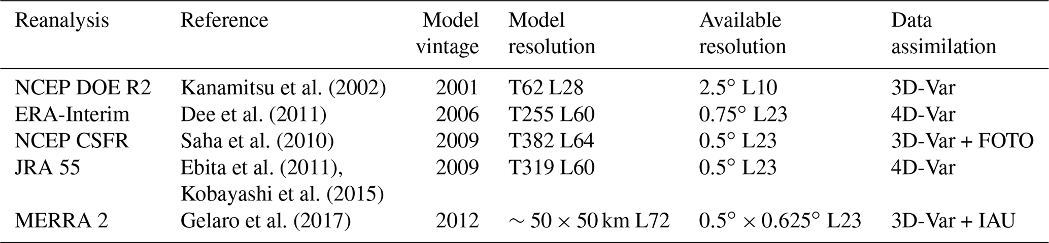
Kanamitsu et al. (2002)Dee et al. (2011)Saha et al. (2010)Ebita et al. (2011)Kobayashi et al. (2015)Gelaro et al. (2017)Table 1Major characteristics of reanalyses compared during the study.
To reduce the ambiguity, we cross-examined the reanalysis moisture transport with the only in situ measurements of humidity and wind – radiosondes – in the footsteps of Connolley and King (1993) and Bromwich et al. (1995). Rather than compute the climatological moisture budget, our contribution will be to investigate the temporal variability of the transport. Radiosoundings cannot provide an independent validation of reanalyses, but they will yield more homogeneous time series. Besides, in Antarctica, humidity soundings are sometimes rejected during the assimilation process, even by state-of-the-art analyses (Barral et al., 2014). Like our predecessors, we restrict ourselves to East Antarctica because of the lack of long-term upper-air measurements in West Antarctica and in the peninsula.
We build upon a similar study in the Arctic (Dufour et al., 2016) and the reanalyses presented herewith. The first NCEP NCAR reanalysis was not included due to a well-known moisture diffusion problem over Antarctica (Cullather et al., 1998) as well as unrealistic evaporation (Hines et al., 1999). Its successor, NCEP DOE R2, solved the main errors from the first attempt (Kanamitsu et al., 2002). At 2.5∘, it has the lowest horizontal resolution of our ensemble (Table 1) as well as the fewest vertical levels. We left out JRA 25 and MERRA 1 because they were not extended to 2016. CFSR has the highest resolution (T382 or approximately 35 km) and includes ocean and sea-ice physics in its forecast model. Our period of study starts in 1980 to adjust to the new reanalysis from NASA and MERRA 2. Among other things, the data assimilation system from MERRA 1 was improved to take into account satellites launched after NOAA-18 (2005), for instance the hyperspectral infrared radiances of EOS Aqua (Gelaro et al., 2017). ERA-Interim and JRA 55 implement 4D-Var assimilation, whereas CFSR and MERRA 2 run improved versions of 3D-Var. ERA-Interim has been commended as especially reliable over Antarctica (Bromwich et al., 2011; Wang et al., 2016).
The domain of the study is constrained by the location of stations running long-term radiosonde programmes, which restricts us to East Antarctica (Fig. 1). SANAE (east of Neumayer) and Molodeznaja (east of Syowa) had practically no humidity soundings available inside our time window. Inland, the radiosonde programme at Vostok Station stopped in 1992; it began at Dome C in 2006 only. The boundary between East and West Antarctica is the transect between the Ross and Filchner-Ronne ice shelves. We excluded ice shelves because they do not contribute to sea-level rise. We smoothed the shape of the domain (red line in Fig. 1) to avoid making the direction normal to the boundary too dependant on the local shape of the coastline (black line). The largest gaps between the stations are at the boundaries between the Ross and Filchner-Ronne ice shelves and around Dumont d'Urville.
Radiosondes can measure moisture advection directly as it is the product of humidity with the horizontal wind vector. The Integrated Global Radiosonde Archive (IGRA) version 2 provided the sounding data (Durre et al., 2006). IGRA stores quality-controlled soundings from more than 2700 stations worldwide dating as far back as 1905. We applied additional climatological checks to the wind and specific humidity variables, similarly to Dufour et al. (2016). Based on monthly distributions, they exclude values further than 3 times the interquartile range from the median. Due to the persistence of unrealistic values, we removed the data from Syowa above 400 hPa.

Figure 1Location of the radiosonde launch sites and boundary of the East Antarctic ice sheet. The diameter of the dots is proportional to the number of archived soundings (maximum is Casey with 39 000 soundings between 1957 and 2016). Only the sites selected for the study are labelled.

Figure 2Monthly density of valid humidity and wind soundings per station and per synoptic time (midnight and noon GMT).
The hygrometers on board radiosondes suffer from known biases some of which can be compensated retrospectively (Miloshevich et al., 2004). For instance, at low temperatures, the hygrometer can no longer adjust to sharp variations in humidity, leading to the so-called time-lag bias. Moreover, the default calibration model of the sensor is inaccurate below −20 ∘C (temperature-dependence error). Unfortunately, the suggested corrections apply only to specific radiosonde models and require metadata and high-resolution vertical data absent from IGRA. However, as we shall see, in Antarctica most of the transport of humidity occurs near the surface, often in warm storm conditions. Finally, solar heating of the sensor also can generate errors which were documented in the case of Antarctica in Rowe et al. (2008) with the help of an Atmospheric Radiance Emitted Interferometer.
The temporal availability of the soundings after filtering is shown in Fig. 2. The temporal sampling is biased against the early 1980s and winters. To build time series and compute trends, we only kept the monthly data of a station if it involved at least 10 valid soundings per month for at least 10 years. The same criterion was used to exclude reanalysis data at given locations and pressure levels that are too often masked due to the topography and variations in surface pressure. When we needed to compare the data sets at specific locations, we co-located the gridded reanalysis data with the stations using bilinear interpolation. In such cases, the year-round 6-hourly reanalysis values were masked to match the irregular availability of observations.
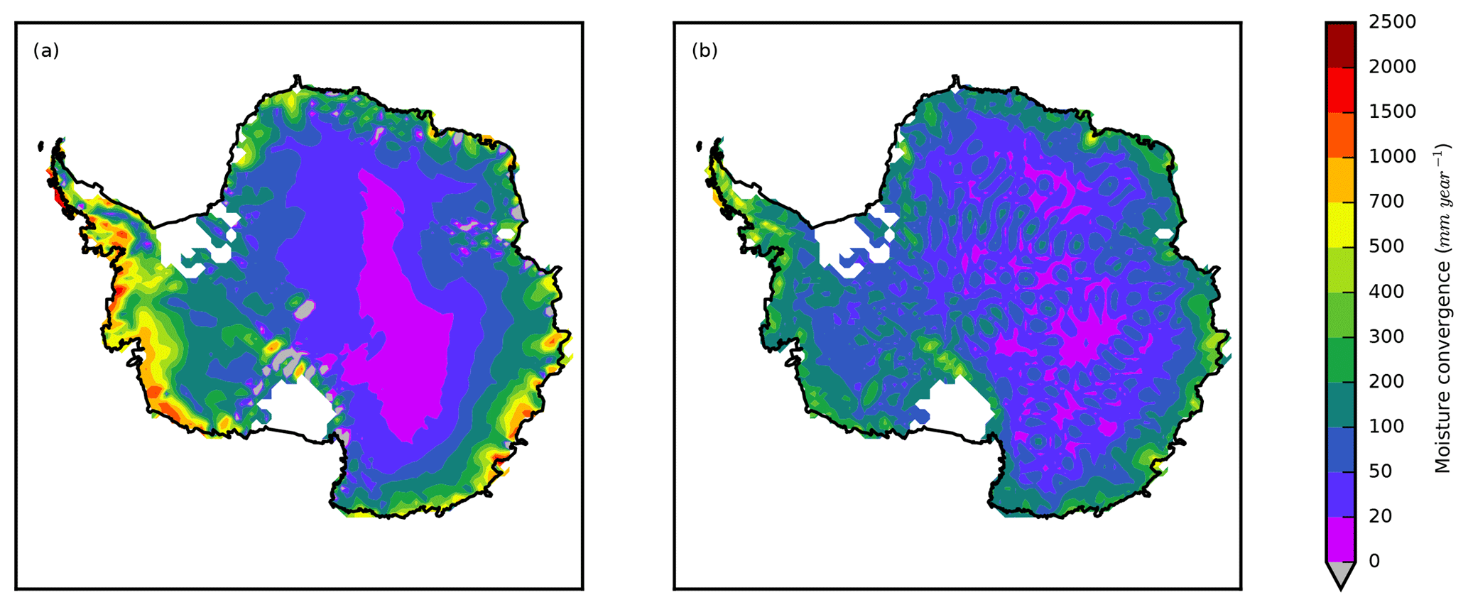
Figure 3Mean vertically integrated moisture flux convergence over Antarctica in ERA-Interim (a) and the standard deviation of that variable for all the studied reanalyses (b).
The study of snow accumulation via upstream atmospheric processes relies on the conservation of water vapour. Over long timescales, the rate of change of precipitable water can be ignored (Peixóto and Oort, 1992) so that the moisture budget equation is reduced to
where E Aa refers to the East Antarctic ice sheet and ∂ to its boundary. ps is the surface pressure, q is the specific humidity and vn is the wind component normal to the boundary. c and e are the condensation and evaporation rates per unit mass. One must then assume that the vertical integral of condensation and evaporation is equal to net precipitation, i.e. that the transport of water only occurs in the gas phase. As it happens, the convergence of cloud frozen and liquid water is in the order of 10 % of the vapour convergence in Antarctica according to the few reanalyses that provide these variables (Dufour, 2016). The final step is to equate net precipitation with snow accumulation. Liquid run-off is indeed negligible given the low temperatures (King and Turner, 2007). Sublimation and hoarfrost will appear under evaporation. However, our method cannot account for snow blown out of the domain by the wind.
We use the trapezoidal rule to approximate the path integrals along the domain boundary, e.g. to compute the left-hand side of Eq. (1). In the case of a variable f available at M stations surrounding the domain this translates to
The lm are the location of the stations after the domain boundary is parameterized by the arc length l. Likewise, the vertical integral of a function f defined on N pressure levels pn is given by
n0 refers to the last pressure level above the surface.
Our aim was to investigate trends rather than absolute amounts so we worked with anomalies with respect to each station's monthly climatology as in Jones (1994). We could thus consider the whole 1980–2016 period and not be as affected by the biased temporal and spatial sampling. Trends and correlations were considered statistically significant for p values higher than 95 % on a two-tail Student t test.
The map of mean moisture convergence in ERA-Interim (Fig. 3a) is broadly similar to the accumulation map in Arthern et al. (2006). The convergence is highest over the peninsula where the westerlies intersect the orography. The lower altitude of West Antarctica allows moisture advection further inland than in the eastern half. The area stretching from Dome Fuji to Dome C receives less than 20 mm of moisture a year.

Figure 4Magnitude of the long-term-averaged (1979–2016) atmospheric moisture budget terms of the East Antarctic ice sheet (a). Linear trends of the moisture budget terms (b): colour indicates rate of change and hatches statistical significance.
Along the coast of East Antarctica and in the Transantarctic Mountains, there are zones of net moisture divergence neighbouring local maxima in excess of 1000 mm yr−1. In comparison, the accumulation from Arthern et al. (2006) is always positive and peaks at 500 mm equivalent water per year. The important wind contrasts in mountain ranges and outlet glaciers are a likely source of numerical artefacts. Theoretically, at least, strong winds erode and sublimate snow, which is a genuine cause of moisture divergence, but these processes are not represented in most climate models (Amory et al., 2015).
Generally speaking, the ensemble standard deviation is proportional to the mean convergence, being highest in the peninsula and along the coast (Fig. 3b). The inter-data-set spread is disproportionately high in the Transantarctic Mountains and the East Antarctic Plateau. The 100 km scale inhomogeneities on the plateau are due to JRA 55. Neither the precipitation nor the evaporation exhibit these features (not shown). Unlike the other data sets, in JRA 55, evaporation is on average negative (net deposition) above 2000 m.
Arthern et al. (2006)Table 2Magnitude of the long-term-averaged (1979–2016) atmospheric moisture budget terms in mm yr−1 for the East Antarctic ice sheet and the whole Antarctic continent (ice-shelves excluded). The columns stand for precipitation (P), evaporation (E), convergence (C), net precipitation (P-E) and residual (P-E-C). Strictly speaking, the values of Arthern et al. (2006) represent accumulation rather than net precipitation. The figure for East Antarctica is a weighted average of the accumulation in the sectors from 45∘ W to 180∘ E.

Given the dispersion between data sets on a local scale, we cannot expect them to converge to a common estimate of convergence on the scale of East Antarctica (Fig. 4a, magenta bars). This is all the more true for evaporation and precipitation, which are forecasted variables and thus even less constrained by observations (light- and dark-blue bars, respectively). One issue with reanalyses is the non-closure of their moisture budget, witnessed by the gap between upper and lower bars in Fig. 4a. The small mismatch in NCEP DOE R2 is illusory, a consequence of its excessively high sublimation (Bromwich et al., 2011). The 4D-Var reanalyses exhibit the smallest residual. The cloud water fluxes were not included: they could improve the balance for CFSR, JRA 55 and MERRA 2 but will worsen it for NCEP DOE R2 and ERA-Interim. For comparison, we also give the break-down of the moisture budget in the case of the whole continent (still excluding ice shelves) in Table 2, along with the figures of Arthern et al. (2006). West Antarctica and the peninsula are more exposed to moisture fluxes, and indeed the convergence is higher for the whole continent. The ranking between reanalyses remains the same.
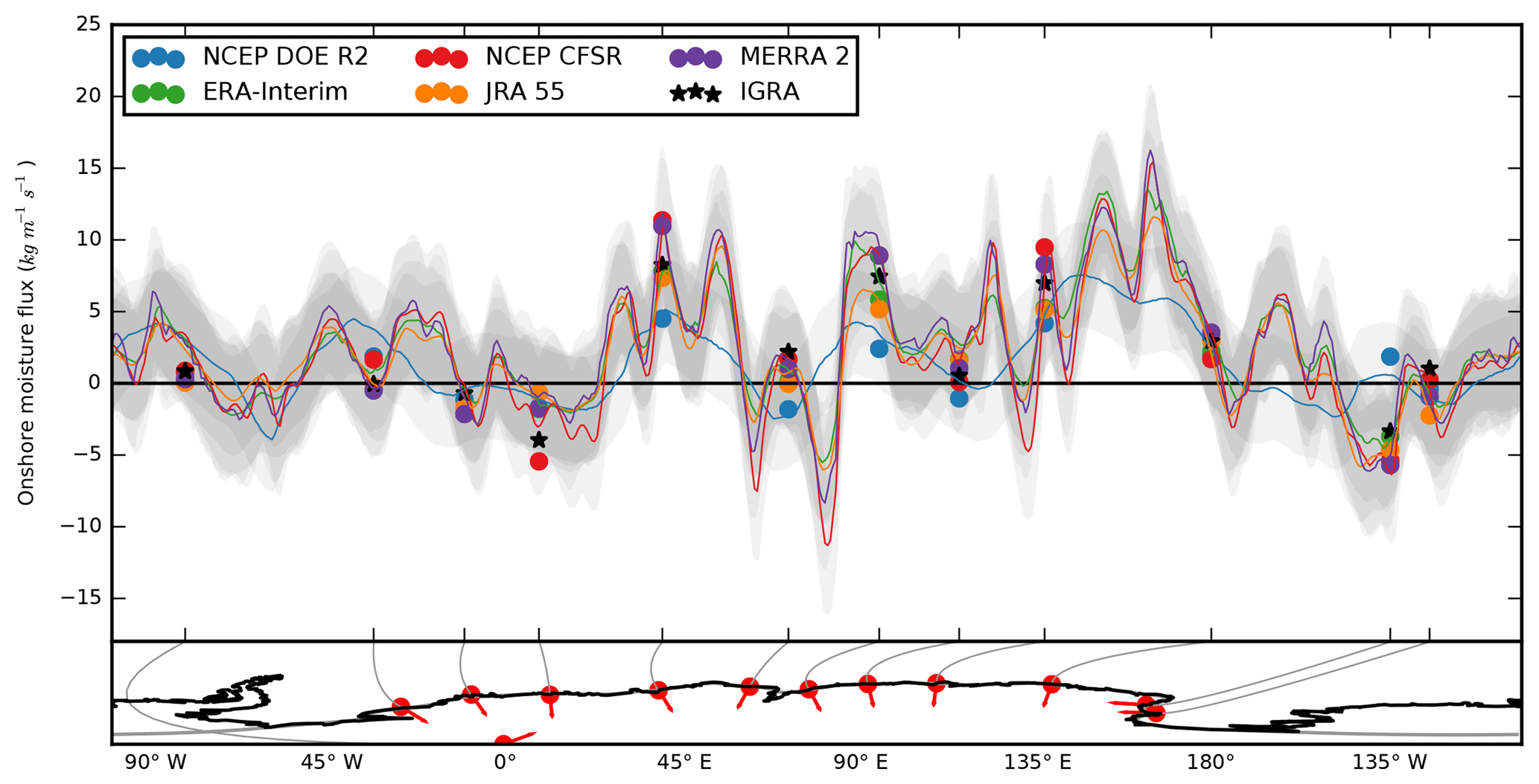
Figure 5Distribution of the mean incoming vertically integrated moisture flux on the boundary of the Antarctic ice sheet in different reanalyses. The grey-shaded bands indicate the ranges corresponding to plus or minus 1 interannual standard deviation from the mean. Stars represent the radiosonde and dots the reanalyses interpolated over the launch sites, with the same temporal sampling as the observations. The red dots in the lower panel indicate the location of the sites and the arrows the direction normal to the boundary.
The interannual variability in reanalyses is doubtful due to the discontinuities introduced by changes in the observation system (Bengtsson et al., 2004). This is especially the case in Antarctica, where analyses rely heavily on satellite data as opposed to conventional observations (Nicolas and Bromwich, 2011). The changes in the components of the moisture budget over time are summarized as linear trends in Fig. 4b. Generally speaking, the trends are weak and inconsistent. Precipitable water has not changed significantly in the modern reanalyses, yet it is the purported mechanism for the future increase in moisture fluxes.
The coastal profile in the upper panel of Fig. 5 was built by interpolating the mean moisture flux field on the smoothed boundary of the East Antarctic ice sheet (lower panel). Overall, the moisture transports are positive over East Antarctica with occasional negative values in valleys where the katabatic winds are channelled, e.g. on the Amery Ice Shelf (70∘ E). Because of its low resolution, NCEP DOE R2 is oblivious to these local effects and is frequently outside of the ensemble envelope. On the other hand, NCEP CFSR, which has the highest spectral resolution (T382), shows stronger offshore fluxes at these locations than ERA-Interim, MERRA 2 and JRA 55.
Above the launch sites, the reanalysis profiles can be compared with the radiosoundings (black stars in Fig. 5). The observations are within the plus or minus 1 standard deviation envelope. In several cases (Syowa, Mawson, Casey), the presence of the radiosounding coincides with an extremum in the reanalysis profile, perhaps a deviation to accommodate the observation.
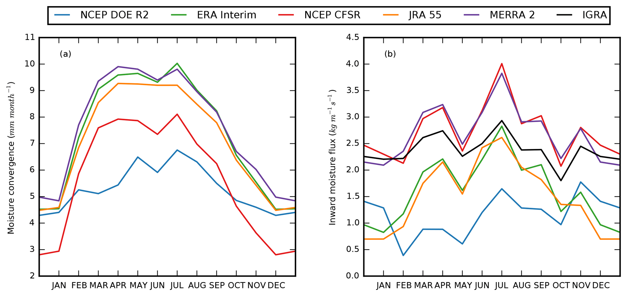
Figure 6Annual cycle of moisture transport into East Antarctica (a) computed from reanalyses averaged over East Antarctica, (b) observations and reanalyses (with the same spatial and temporal sampling) averaged over all stations.
The reanalysis climatology is built on 6-hourly data, whereas there are two radiosoundings a day at the very best with extensive gaps in the data. To correct the sampling bias, we now only consider the reanalysis time steps that coincide with a radiosounding. The resulting time averages are shown as dots in Fig. 5. As expected, there is a gap between profiles and the dots, a measure of the sampling bias. This is particulary true for Mirny as well as for Novolazarevskaya in the case of NCEP CFSR. The values for South Pole Station are shown at the abscissa of the closest point on the domain boundary; the direction of fluxes normal to the boundary is also defined at this point. At the South Pole, the difference between profiles and dots is also a consequence of the distance to the boundary. Otherwise, the subsampled reanalyses are quite representative of the year-round values, including the summer-only data at Mario Zucchelli Station, surprisingly.
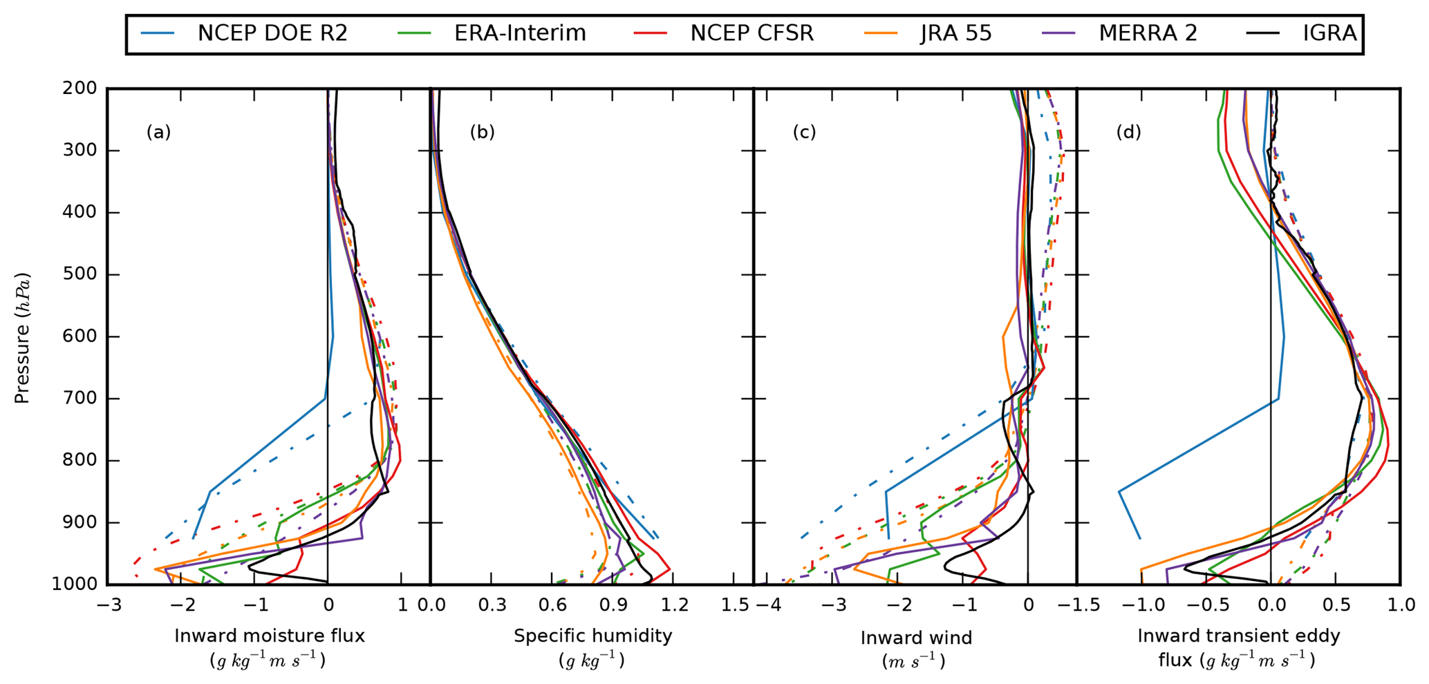
Figure 7Mean vertical profiles over radiosonde sites, simultaneously with observations (solid lines); along the coast of the East Antarctic ice sheet for the whole 1980–2016 period (dashed lines). The variables displayed in the panels are moisture flux (a), specific humidity (b), mean wind (c) and transient eddy fluxes (d).
This is likely a coincidence: the annual cycle of moisture convergence experiences a two-fold increase during the austral winter (Fig. 6a). In the Southern Hemisphere, the lower winter humidity is more than compensated by the stronger storm activity (Oshima and Yamazaki, 2006). NCEP DOE R2 has a much weaker convergence cycle perhaps due to the unrealistic evaporation in summer. When the reanalyses are interpolated on the stations and masked in time to match the radiosonde launches, the annual cycle is quite different (Fig. 6b). The transition from summer to winter is no longer as sharp in most data sets and it is altogether absent from NCEP DOE R2 and IGRA.
In the vertical, the moisture flux profiles demonstrate two different regimes (Fig. 7a). In most data sets, including observations, the transport changes polarity around 900 hPa: into the continent above and away from it below. The level of the transition is higher in ERA-Interim (850 hPa) and higher still in NCEP DOE R2 (750–700 hPa). The 1000 hPa level in NCEP DOE R2 was too often below the ground to be shown. The surface fluxes are weaker above stations (solid lines) than in the continental average (dashed lines).
The inter-data-set spread also increases near the surface in the case of humidity (Fig. 7b). The IGRA observations exhibit a shallow inversion that is also present in the modern reanalyses but deeper and stronger. There is practically no mean wind above 800 hPa, but below the prevailing winds blow out from the ice sheet. This is the signature of katabatic flows. There is some difference between the original reanalyses and when they are both sampled in time and interpolated in space. We suggest that the stations are not representative of their surroundings because they were generally built in places sheltered from the winds. Only the high-resolution data sets can represent both the katabatic outflow and the relative haven of the station. What is more, the radiosonde launch is more likely to be cancelled or the balloon may be lost during a strong katabatic event, which biases the observations against these conditions.
Due to the correlation between wind and humidity, the mean moisture flux () is more than the product of the mean wind () and the mean humidity (). The residual is the transient eddy term of the Reynolds decomposition: . In the presence of an extratropical cyclone, the warm sector advects exceptionally moist air inland and vice versa in its cold sector. This corresponds to the inward fluxes above 900 hPa in Fig. 7d. They peak at 750 hPa and then decrease with altitude. Below 900 hPa, the fluxes averaged along the boundary remain positive, but they change polarity at the sonde locations. Intermittent katabatic conditions imply unusually strong downslope winds: they will lead to positive transient eddy fluxes if they advect the unusually dry air from the plateau. However, they will count as negative if that air is moistened by the sublimation of blowing snow (Barral et al., 2014) or precipitation (Grazioli et al., 2017). The former process, at least, is not modelled in the reanalyses. Its effect on the humidity profile will only be felt where radiosoundings are assimilated. Returning to panel (a), we now interpret the outward low-level fluxes as the effect of katabatic winds, but we suspect that this effect is underestimated for different reasons depending on the location. At the stations, the prevailing katabatic wind is weaker than average. Away from the observations, the reanalyses are too dry during katabatic events. The inward high-level fluxes are a consequence of transient eddies, presumably extratropical cyclones, with good agreement between sites and data sets.
We finish the intercomparison with the statistical distributions of vertically integrated moisture transport, both in the non-sampled and subsampled cases (Fig. 8a and b). The positive (inward) transport dominates, particularly the last decile, but the negative (outgoing) fluxes are nonetheless important: they comprise more than a third of the absolute transport. The inter-data-set variability is as strong for the positive and the negative transport, highlighting once more the role of katabatic winds. In the subsampled case, the observations fall within the reanalysis envelope, but the inter-data-set variability is also greater.
To sum up, radiosondes and reanalyses diverge in narrow valleys and near the ground, especially for low-resolution models. Otherwise, since radiosondes are usually assimilated into reanalyses, the difference between the two is predictably small. The added value of radiosondes is the study of time series.
Time series from reanalyses reflect modifications to the observation system in addition to changes in the climate. The radiosonde record also has its homogeneity issues, e.g. when instruments are upgraded. These events are recorded in the IGRA metadata and we found no association with discontinuities in the times series. We will therefore interpret sudden divergences between observations and reanalyses as artefacts of the data assimilation. From Fig. 9, the most conspicuous ones are in NCEP DOE R2, followed by JRA 55, but they do not take the form of the shifts we would expect with, say, the introduction of a new satellite. Rather, anomalies are amplified intermittently compared to observations or one reanalysis departs for several years from the ensemble. At Amundsen Scott Station (South Pole), observations exhibit variations in higher amplitude than the reanalyses. The extreme climate in our only inland station must have been a test to both measurements and reanalyses.
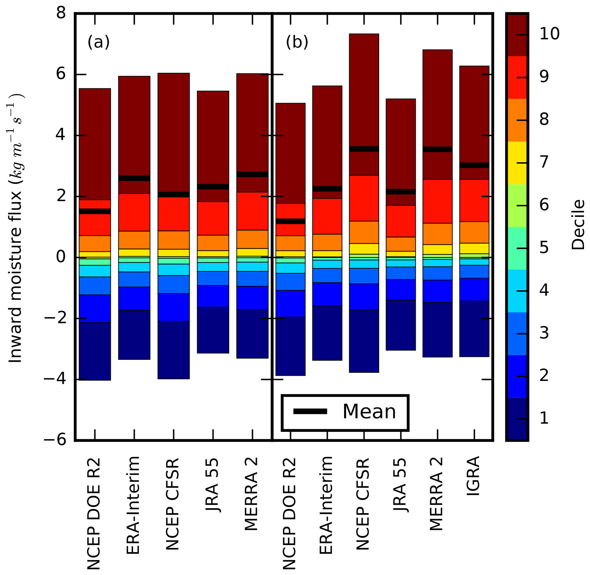
Figure 8Breakdown of the climatological vertically integrated moisture flux into the contribution of its different deciles. When a decile is represented below the origin, its contribution is negative. The top of the bar indicates the mean transport when negative values are set to zero. The difference between the top and bottom is the mean transport, symbolized by the bold black line. In panel (a), the flux deciles are averaged over the East Antarctic boundary, whereas in panel (b) the deciles are computed by aggregating the data over stations only with the same temporal sampling as IGRA.

Figure 9Time series of vertically integrated moisture transport anomalies into East Antarctica (in kg m−1 s−1) at the location of the selected stations in observations and reanalyses.
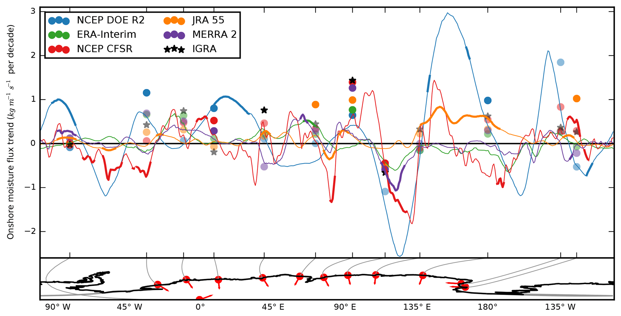
Figure 10Linear trends of vertically integrated moisture transport into East Antarctica. The profiles are built from reanalyses over the 1980–2016 period interpolated along the domain boundary, whereas the dots are computed from reanalyses with the same temporal sampling as the observations. The stars correspond to trends computed from observations. The bold sections of the profiles and the solid dots and stars indicate statistically significant changes.
We now examine the long-term evolution of moisture transport in terms of linear trends, this time analysed along the horizontal dimension (Fig. 10). Most longitudes show no statistically significant change in the advection. Among those that do, even fewer display an agreement between data sets. Mirny Station and its surroundings to the east have seen less moisture travelling inland according to the observations, NCEP CFSR and MERRA 2. The other reanalyses agree in polarity but not in significance. There has been a similar decrease over the Amery Ice Shelf between Davis and Mawson stations. The radiosondes and the interpolated reanalyses at Mawson Station present an opposite trend, which is greater in magnitude than the uninterpolated reanalyses, indicating a sampling bias. This increase evokes the accumulation measurements of Ding et al. (2015) on the eastern side of the nearby Lambert Glacier, but it is unrelated: the timing of the rise is off by a decade. Radiosondes at Syowa Station report an increase in the onshore moisture flux that is stronger than the reanalyses. Syowa Station is located at the edge of the domain surrounding Kohnen Station, identified in Boening et al. (2012) and where ice cores have revealed a similar increase in accumulation. In Adélie Land, trends are incoherent in polarity. The positive trend in radiosondes is not significantly different from zero, in line with the findings of Agosta et al. (2012). Van Ommen and Morgan (2010) recorded anomalous precipitation at Law Dome that peaked in the mid-1970s before returning to normal by the turn of the century, but there is no trace of this trend in the observed transport at the nearby station of Casey. The decreasing accumulation in Victoria Land from Thomas et al. (2017) is not apparent in the time series of McMurdo and Mario Zucchelli stations, presumably because the ice core sites were located further north.
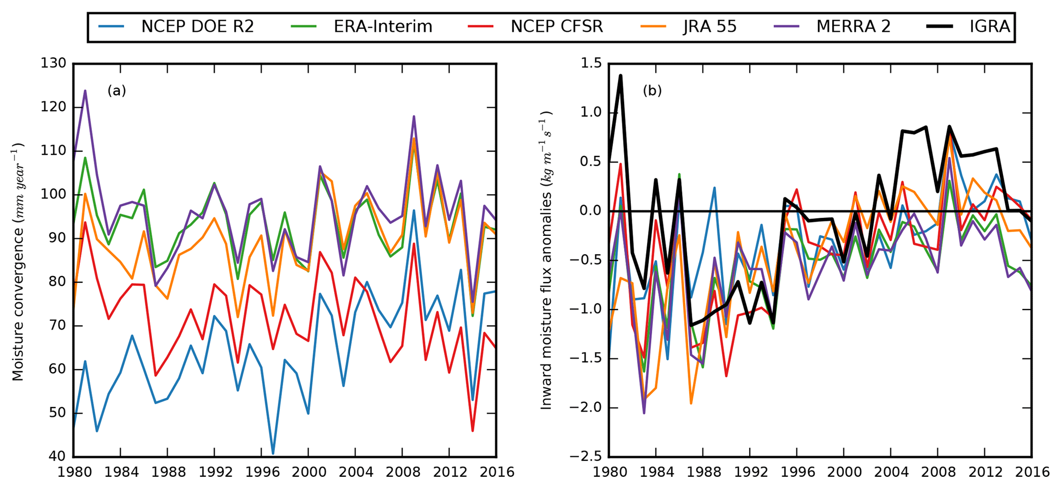
Figure 11Time series of transport into East Antarctica: (a) absolute amounts computed from reanalyses averaged over the domain boundary, (b) anomalies of observations and reanalyses (with the same spatial and temporal sampling) averaged over all stations.
On the scale of the ice sheet, we know from Fig. 4 that the transport series from reanalyses will be offset by up to 30 mm yr−1 and that they will present contradictory trends. In Fig. 11a, ERA-Interim, JRA 55 and MERRA 2 are grouped together, especially after 2000. NCEP DOE R2 is once again the outlier. It is the only data set to not peak in 1980. Surprisingly, NCEP CFSR diverges from the other modern reanalyses in the 1980s.
When we restrict the reanalyses to the locations and times of radiosonde launches, they display a more consistent behaviour (Fig. 11b): a downward trend in the 1980s and an upward trend in the two following decades. Observations follow the same pattern with comparatively higher fluxes in the 1980s and 2000s. During the same period, precipitable water above the launch sites has remained constant, both in observations and analyses (not shown). The interdecadal pattern in transport is therefore a consequence of variable winds rather than thermodynamics.
From Fig. 11b, we deduce a straightforward assimilation of radiosoundings by reanalyses when available. The reanalysis time series at the stations would be less consistent if the assimilation relied more on the model first guess or on remote-sensing data. While the time series at the stations may be accurate, they would be irrelevant if they were not representative of East Antarctica as a whole. If that were the case, the two panels of Fig. 11 would have little in common. As we saw, this true of is decadal variability. However once trends are removed, the continental and the station detrended time series are significantly correlated on a year-to-year basis for all reanalyses except NCEP DOE R2. The significant correlation coefficients lie between 0.48 (JRA 55) and 0.61 (MERRA 2). This gives credibility to the claim that the network of stations is representative of the entire boundary of the ice sheet.
We have compared moisture transport to Antarctica in five reanalyses and over the 1980–2016 period. For East Antarctica, estimates of moisture convergence range from 65 to 96 mm yr−1 and net precipitation from 60 to 123 mm yr−1 (respectively 72–96 and 91–123 mm yr−1 when excluding NCEP DOE R2). The polarity of the linear trend for moisture convergence is not consistent. In any case, changes are not driven by precipitable water increases.
The scarce situ observations and the unreliable satellite observations (Bouchard et al., 2010) make Antarctica a fitting object of study for reanalyses. The differences we found between the data sets remind us of their familiar limitations: model dependence in the absence of observations and unreliable time series (Bromwich et al., 2011; Nicolas and Bromwich, 2011). Additionally, the non-closure of their atmospheric hydrological budget is an issue for estimating accumulation over the ice sheet. Fortunately, the gap between moisture convergence and net precipitation is reduced by 4D-Var assimilation.
Although radiosondes are assimilated by reanalyses, lower-resolution models have difficulties in taking into account observations near the surface and on irregular terrain. This is relevant to representing the humidity inversion and how valleys funnel moisture offshore during katabatic events. Most of the onshore moisture transport occurs above 950 hPa as transient eddy fluxes and in winter. This consistently represented in all but the oldest reanalysis.
Changes in the observing system confounds the interpretation of temporal variability in reanalyses. At the cost of spatial coverage, the original observations provide a homogeneous time series that can be used as a proxy for accumulation. After a sharp decline in the 1980s, the moisture transport recovered gradually in the 1990s and early 2000s and has since slightly decreased. This time series can now serve as a reference for identifying spurious trends in the reanalyses.
The seasonal resolution of stake farms and ice cores is not enough to study short and intense accumulation events such as those described in Gorodetskaya et al. (2014), but radiosondes are launched on a daily basis. The distribution of moisture transport highlights both positive and negative extreme events. Regarding exports, the conflation of net precipitation with accumulation ignores wind erosion in particular. The reanalyses only represent its signature on the humidity profile near radiosonde sites. Conversely, the observations are made in sheltered locations that experience a weaker transport by the mean wind.
In the long term and averaged over all the selected East Antarctic stations, there has been no statistically significant increase, either in incoming moisture or in precipitable water. In contrast, surface temperature trends are much stronger in West Antarctica and the peninsula (Steig et al., 2009), with probable consequences for the moisture budget. It remains to be seen whether the limited radiosonde data in these regions can provide the corresponding evidence.
The reanalysis data sets were available by courtesy of NCEP, JMA, ECMWF and NASA. In practice, the NCEP reanalyses and JRA 55 were found at https://rda.ucar.edu/ (Schuster et al., 2019), ERA-Interim at https://www.ecmwf.int/en/forecasts (Berrisford et al., 2019) and MERRA 2 at https://disc.gsfc.nasa.gov/ (Pham and Hedge, 2019). The IGRA sounding data were made available by the NOAA National Centers for Environmental Information at ftp://ftp.ncdc.noaa.gov/pub/data/igra (Durre, 2019).
The bulk of the article was completed as part of AD's PhD thesis under the supervision of OZ. CC contributed specifically to the question of biases in humidity soundings.
The authors declare that they have no conflict of interest.
This work was supported by the project
“Mechanisms of moisture advection in high latitudes in the present and
future climate” funded by CNRS, IGE and UGA and partly through the BELMONT
Forum Fund ARCTIC-ERA project funded by ANR. Olga Zolina also benefited from the
project 14.613.21.0083 (ID RFMEFI61317X0083) funded by the Ministry of
Education and Science of Russia. We are grateful to the logistics crew at Cap
Prudhomme, Vincent Favier and the TA64 Météo France team, particularly
Didier Lacoste for investigating the station's present weather archives on
our behalf. Finally, we thank the editor and the two anonymous reviewers for their consideration and constructive comments.
Edited by: Christian Beer
Reviewed by: two anonymous referees
Agosta, C., Favier, V., Genthon, C., Gallée, H., Krinner, G., Lenaerts, J. T., and van den Broeke, M. R.: A 40-year accumulation dataset for Adelie Land, Antarctica and its application for model validation, Clim. Dynam., 38, 75–86, 2012. a, b, c
Amory, C., Trouvilliez, A., Gallée, H., Favier, V., Naaim-Bouvet, F., Genthon, C., Agosta, C., Piard, L., and Bellot, H.: Comparison between observed and simulated aeolian snow mass fluxes in Adélie Land, East Antarctica, The Cryosphere, 9, 1373–1383, https://doi.org/10.5194/tc-9-1373-2015, 2015. a
Arthern, R. J., Winebrenner, D. P., and Vaughan, D. G.: Antarctic snow accumulation mapped using polarization of 4.3-cm wavelength microwave emission, J. Geophys. Res.-Atmos., 111, D06107, https://doi.org/10.1029/2004JD005667, 2006. a, b, c, d, e, f
Barral, H., Genthon, C., Trouvilliez, A., Brun, C., and Amory, C.: Blowing snow in coastal Adélie Land, Antarctica: three atmospheric-moisture issues, The Cryosphere, 8, 1905–1919, https://doi.org/10.5194/tc-8-1905-2014, 2014. a, b
Bengtsson, L., Hagemann, S., and Hodges, K. I.: Can climate trends be calculated from reanalysis data?, J. Geophys. Res.-Atmos., 109, D11111, https://doi.org/10.1029/2004JD004536, 2004. a
Bengtsson, L., Hodges, K. I., Koumoutsaris, S., Zahn, M., and Keenlyside, N.: The changing atmospheric water cycle in polar regions in a warmer climate, Tellus A, 63, 907–920, 2011. a
Berrisford, P., Dee, D. P., Poli, P., Brugge R., Fielding, M., Fuentes, M., Kållberg, P. W., Kobayashi S., Uppala, S., and Simmons, A.: The ERA-Interim archive Version 2.0, available at: https://www.ecmwf.int/en/forecasts, last access: 28 January 2019. a
Boening, C., Lebsock, M., Landerer, F., and Stephens, G.: Snowfall-driven mass change on the East Antarctic Ice Sheet, Geophys. Res. Lett., 39, L21501, https://doi.org/10.1029/2012GL053316, 2012. a, b
Bouchard, A., Rabier, F., Guidard, V., and Karbou, F.: Enhancements of satellite data assimilation over Antarctica, Mon. Weather Rev., 138, 2149–2173, 2010. a
Bromwich, D. H., Robasky, F. M., Cullather, R. I., and Van Woert, M. L.: The atmospheric hydrologic cycle over the Southern Ocean and Antarctica from operational numerical analyses, Mon. Weather Rev., 123, 3518–3538, 1995. a
Bromwich, D. H., Nicolas, J. P., and Monaghan, A. J.: An Assessment of Precipitation Changes over Antarctica and the Southern Ocean since 1989 in Contemporary Global Reanalyses, J. Climate, 24, 4189–4209, 2011. a, b, c, d
Collins, M., Knutti, R., Arblaster, J., Dufresne, J.-L., Fichefet, T., Friedlingstein, P., Gao, X., Gutowski, W., Johns, T., Krinner, G., Shongwe, M., Tebaldi, C., Weaver, A., and Wehner, M.: Long-term Climate Change: Projections, Commitments and Irreversibility, book section 12, 1029–1136, Cambridge University Press, Cambridge, UK and New York, NY, USA, 2013. a
Connolley, W. and King, J.: Atmospheric water-vapour transport to Antarctica inferred from radiosonde data, Q. J. Roy. Meteor. Soc., 119, 325–342, 1993. a
Cullather, R. I., Bromwich, D. H., and Van Woert, M. L.: Spatial and Temporal Variability of Antarctic Precipitation from Atmospheric Methods, J. Climate, 11, 334–367, 1998. a
Dee, D., Uppala, S., Simmons, A., Berrisford, P., Poli, P., Kobayashi, S., Andrae, U., Balmaseda, M., Balsamo, G., Bauer, P., Bechtold, P., Beljaars, A. C. M., van de Berg, L., Bidlot, J., Bormann, N., Delsol, C., Dragani, R., Fuentes, M., Geer, A. J., Haimberger, L., Healy, S. B., Hersbach, H., Hólm, E. V., Isaksen, L., Kållberg, P., Köhler, M., Matricardi, M., McNally, A. P., Monge-Sanz, B. M., Morcrette, J.-J., Park, B.-K., Peubey, C., de Rosnay, P., Tavolato, C., Thépaut, J.-N. and Vitart, F.: The ERA-Interim reanalysis: configuration and performance of the data assimilation system, Q. J. Roy. Meteor. Soc., 137, 553–597, 2011. a
Ding, M., Xiao, C., Li, C., Qin, D., Jin, B., Shi, G., Xie, A., and Cui, X.: Surface mass balance and its climate significance from the coast to Dome A, East Antarctica, Sci. China Earth Sci., 58, 1787–1797, 2015. a, b
Dufour, A.: Transport de vapeur d'eau vers les hautes latitudes: Mécanismes et variabilité d'après réanalyses et radiosondages, PhD thesis, Grenoble Alpes, Grenoble, France, 2016. a
Dufour, A., Zolina, O., and Gulev, S. K.: Atmospheric Moisture Transport to the Arctic: Assessment of Reanalyses and Analysis of Transport Components, J. Climate, 29, 5061–5081, 2016. a, b
Durre, I.: Integrated Global Radiosonde Archive, available at: ftp://ftp.ncdc.noaa.gov/pub/data/igra, last access: 28 January 2019. a
Durre, I., Vose, R. S., and Wuertz, D. B.: Overview of the Integrated Global Radiosonde Archive, J. Climate, 19, 53–68, 2006. a
Ebita, A., Kobayashi, S., Ota, Y., Moriya, M., Kumabe, R., Onogi, K., Harada, Y., Yasui, S., Miyaoka, K., Takahashi, K., Kamahori, H., Kobayashi, C., Endo, H., Soma, M., Oikawa, Y., and Ishimizu, T.: The Japanese 55-year reanalysis “JRA-55”: an interim report, Sola, 7, 149–152, 2011. a
Eisen, O., Frezzotti, M., Genthon, C., Isaksson, E., Magand, O., van den Broeke, M. R., Dixon, D. A., Ekaykin, A., Holmlund, P., Kameda, T., Karlöf, L., Kaspari, S., Lipenkov, V. Y., Oerter, H., Takahashi, S., and Vaughan, D. G.: Ground-based measurements of spatial and temporal variability of snow accumulation in East Antarctica, Rev. Geophys., 46, RG2001, https://doi.org/10.1029/2006RG000218, 2008. a
Favier, V., Agosta, C., Parouty, S., Durand, G., Delaygue, G., Gallée, H., Drouet, A.-S., Trouvilliez, A., and Krinner, G.: An updated and quality controlled surface mass balance dataset for Antarctica, The Cryosphere, 7, 583–597, https://doi.org/10.5194/tc-7-583-2013, 2013. a
Fretwell, P., Pritchard, H. D., Vaughan, D. G., Bamber, J. L., Barrand, N. E., Bell, R., Bianchi, C., Bingham, R. G., Blankenship, D. D., Casassa, G., Catania, G., Callens, D., Conway, H., Cook, A. J., Corr, H. F. J., Damaske, D., Damm, V., Ferraccioli, F., Forsberg, R., Fujita, S., Gim, Y., Gogineni, P., Griggs, J. A., Hindmarsh, R. C. A., Holmlund, P., Holt, J. W., Jacobel, R. W., Jenkins, A., Jokat, W., Jordan, T., King, E. C., Kohler, J., Krabill, W., Riger-Kusk, M., Langley, K. A., Leitchenkov, G., Leuschen, C., Luyendyk, B. P., Matsuoka, K., Mouginot, J., Nitsche, F. O., Nogi, Y., Nost, O. A., Popov, S. V., Rignot, E., Rippin, D. M., Rivera, A., Roberts, J., Ross, N., Siegert, M. J., Smith, A. M., Steinhage, D., Studinger, M., Sun, B., Tinto, B. K., Welch, B. C., Wilson, D., Young, D. A., Xiangbin, C., and Zirizzotti, A.: Bedmap2: improved ice bed, surface and thickness datasets for Antarctica, The Cryosphere, 7, 375–393, https://doi.org/10.5194/tc-7-375-2013, 2013. a
Fyke, J., Lenaerts, J. T. M., and Wang, H.: Basin-scale heterogeneity in Antarctic precipitation and its impact on surface mass variability, The Cryosphere, 11, 2595–2609, https://doi.org/10.5194/tc-11-2595-2017, 2017. a
Gelaro, R., McCarty, W., Suárez, M. J., Todling, R., Molod, A., Takacs, L., Randles, C., Darmenov, A., Bosilovich, M. G., Reichle, R., Wargan, K., Coy, L., Cullather, R., Draper, C., Akella, S., Buchard, V., Conaty, A., da Silva, A. M., Gu, W., Kim, G., Koster, R., Lucchesi, R., Merkova, D., Nielsen, J. E., Partyka, G., Pawson, S., Putman, W., Rienecker, M., Schubert, S. D., Sienkiewicz, M., and Zhao, B.: The Modern-Era Retrospective Analysis for Research and Applications, Version 2 (MERRA-2), J. Climate, 30, 5419–5454, https://doi.org/10.1175/JCLI-D-16-0758.1, 2017. a, b
Genthon, C. and Krinner, G.: Convergence and disposal of energy and moisture on the Antarctic polar cap from ECMWF reanalyses and forecasts, J. Climate, 11, 1703–1716, 1998. a
Gorodetskaya, I. V., Tsukernik, M., Claes, K., Ralph, M. F., Neff, W. D., and Van Lipzig, N. P.: The role of atmospheric rivers in anomalous snow accumulation in East Antarctica, Geophys. Res. Lett., 41, 6199–6206, 2014. a
Grazioli, J., Madeleine, J.-B., Gallée, H., Forbes, R. M., Genthon, C., Krinner, G., and Berne, A.: Katabatic winds diminish precipitation contribution to the Antarctic ice mass balance, P. Natl. Acad. Sci. USA, 114, 10858–10863, https://doi.org/10.1073/pnas.1707633114, 2017. a
Hines, K. M., Grumbine, R. W., Bromwich, D. H., and Cullather, R. I.: Surface Energy Balance of the NCEP MRF and NCEP-NCAR Reanalysis in Antarctic Latitudes during FROST, Weather Forecast., 14, 851–866, 1999. a
Jones, P. D.: Hemispheric surface air temperature variations: a reanalysis and an update to 1993, J. Climate, 7, 1794–1802, 1994. a
Kanamitsu, M., Ebisuzaki, W., Woollen, J., Yang, S.-K., Hnilo, J., Fiorino, M., and Potter, G.: NCEP-DOE AMIP-II Reanalysis (R-2), B. Am. Meteorol. Soc., 83, 1631–1643, 2002. a, b
King, J. C. and Turner, J.: Antarctic meteorology and climatology, Cambridge University Press, Cambridge, UK, 2007. a
Kobayashi, S., Ota, Y., Harada, Y., Ebita, A., Moriya, M., Onoda, H., Onogi, K., Kamahori, H., Kobayashi, C., Endo, H., Miyaoka, K., and Takahashi K.: The JRA-55 reanalysis: general specifications and basic characteristics, J. Meteorol. Soc. Jpn., 93, 5–48, 2015. a
Lenaerts, J., Den Broeke, M., Berg, W., Meijgaard, E. v., and Kuipers Munneke, P.: A new, high-resolution surface mass balance map of Antarctica (1979–2010) based on regional atmospheric climate modeling, Geophys. Res. Lett., 39, L04501, https://doi.org/10.1029/2011GL050713, 2012. a, b
Medley, B., McConnell, J., Neumann, T., Reijmer, C., Chellman, N., Sigl, M., and Kipfstuhl, S.: Temperature and snowfall in western Queen Maud Land increasing faster than climate model projections, Geophys. Res. Lett., 45, 1472–1480, 2018. a
Miloshevich, L. M., Paukkunen, A., Vömel, H., and Oltmans, S. J.: Development and validation of a time-lag correction for Vaisala radiosonde humidity measurements, J. Atmos. Ocean. Tech., 21, 1305–1327, 2004. a
Monaghan, A. J., Bromwich, D. H., Fogt, R. L., Wang, S.-H., Mayewski, P. A., Dixon, D. A., Ekaykin, A., Frezzotti, M., Goodwin, I., Isaksson, E., Kaspari, S. D., Morgan, V. I., Oerter, H., Van Ommen, T. D., Van der Veen, C. J., and Wen, J.: Insignificant change in Antarctic snowfall since the International Geophysical Year, Science, 313, 827–831, 2006. a, b
Nicolas, J. P. and Bromwich, D. H.: Precipitation changes in high southern latitudes from global reanalyses: A cautionary tale, Surv. Geophys., 32, 475–494, 2011. a, b, c
Oshima, K. and Yamazaki, K.: Difference in seasonal variation of net precipitation between the Arctic and Antarctic regions, Geophys. Res. Lett., 33, L18501, https://doi.org/10.1029/2006GL027389, 2006. a
Palerme, C., Kay, J. E., Genthon, C., L'Ecuyer, T., Wood, N. B., and Claud, C.: How much snow falls on the Antarctic ice sheet?, The Cryosphere, 8, 1577–1587, https://doi.org/10.5194/tc-8-1577-2014, 2014. a
Palerme, C., Genthon, C., Claud, C., Kay, J. E., Wood, N. B., and L'Ecuyer, T.: Evaluation of current and projected Antarctic precipitation in CMIP5 models, Clim. Dynam., 48, 225–239, 2017. a
Peixóto, J. and Oort, A. H.: Physics of climate, American institute of physics, New York, USA, 1992. a
Pham, L. and Hedge, M.: Goddard Earth Sciences Data and Information Services Center, available at: https://disc.gsfc.nasa.gov/, last access: 28 January 2019. a
Rowe, P. M., Miloshevich, L. M., Turner, D. D., and Walden, V. P.: Dry bias in Vaisala RS90 radiosonde humidity profiles over Antarctica, J. Atmos. Ocean. Tech., 25, 1529–1541, 2008. a
Saha, S., Moorthi, S., Pan, H.-L., Wu, X., Wang, J., Nadiga, S., Tripp, P., Kistler, R., Woollen, J., Behringer, D., Liu, H., Stokes, D., Grumbine, R., Gayno, G., Wang, J., Hou, Y., Chuang, H., Juang, H. H., Sela, J., Iredell, M., Treadon, R., Kleist, D., Van Delst, P., Keyser, D., Derber, J., Ek, M., Meng, J., Wei, H., Yang, R., Lord, S., van den Dool, H., Kumar, A., Wang, W., Long, C., Chelliah, M., Xue, Y., Huang, B., Schemm, J., Ebisuzaki, W., Lin, R., Xie, P., Chen, M., Zhou, S., Higgins, W., Zou, C., Liu, Q., Chen, Y., Han, Y., Cucurull, L., Reynolds, R. W., Rutledge, G., and Goldberg, M.: The NCEP Climate Forecast System Reanalysis, B. Am. Meteorol. Soc., 91, 1015–1057, 2010. a
Schuster, D., Banner, C., Conroy, R., Cram, T., Dattore, B., Hou, S., Ji, Z., Ramos, C., Shih, C. F., Stepaniak, D., and Worley, S.: NCAR's Research Data Archive, available at: https://rda.ucar.edu/, last access: 28 January 2019. a
Steig, E. J., Schneider, D. P., Rutherford, S. D., Mann, M. E., Comiso, J. C., and Shindell, D. T.: Warming of the Antarctic ice-sheet surface since the 1957 International Geophysical Year, Nature, 457, 459–462, 2009. a
Thomas, E. R., van Wessem, J. M., Roberts, J., Isaksson, E., Schlosser, E., Fudge, T. J., Vallelonga, P., Medley, B., Lenaerts, J., Bertler, N., van den Broeke, M. R., Dixon, D. A., Frezzotti, M., Stenni, B., Curran, M., and Ekaykin, A. A.: Regional Antarctic snow accumulation over the past 1000 years, Clim. Past, 13, 1491–1513, https://doi.org/10.5194/cp-13-1491-2017, 2017. a, b
Tsukernik, M. and Lynch, A. H.: Atmospheric meridional moisture flux over the Southern Ocean: A story of the Amundsen Sea, J. Climate, 26, 8055–8064, 2013. a
Van Ommen, T. D. and Morgan, V.: Snowfall increase in coastal East Antarctica linked with Southwest Western Australian drought, Nat. Geosci., 3, 267–272, 2010. a, b
Wang, Y., Ding, M., van Wessem, J. M., Schlosser, E., Altnau, S., van den Broeke, M. R., Lenaerts, J. T. M., Thomas, E. R., Isaksson, E., Wang, J., and Sun, W.: A Comparison of Antarctic Ice Sheet Surface Mass Balance from Atmospheric Climate Models and In Situ Observations, J. Climate, 29, 5317–5337, https://doi.org/10.1175/JCLI-D-15-0642.1, 2016. a