the Creative Commons Attribution 4.0 License.
the Creative Commons Attribution 4.0 License.
 | 08 Nov 2019
Wave energy attenuation in fields of colliding ice floes – Part 2: A laboratory case study
Sukun Cheng
Hayley H. Shen
This work analyses laboratory observations of wave energy attenuation in fragmented sea ice cover composed of interacting, colliding floes. The experiment, performed in a large (72 m long) ice tank, includes several groups of tests in which regular, unidirectional, small-amplitude waves of different periods were run through floating ice with different floe sizes. The vertical deflection of the ice was measured at several locations along the tank, and video recording was used to document the overall ice behaviour, including the presence of collisions and overwash of the ice surface. The observational data are analysed in combination with the results of two types of models: a model of wave scattering by a series of floating elastic plates, based on the matched eigenfunction expansion method (MEEM), and a coupled wave–ice model, based on discrete-element model (DEM) of sea ice and a wave model solving the stationary energy transport equation with two source terms, describing dissipation due to ice–water drag and due to overwash. The observed attenuation rates are significantly larger than those predicted by the MEEM model, indicating substantial contribution from dissipative processes. Moreover, the dissipation is frequency dependent, although, as we demonstrate in the example of two alternative theoretical attenuation curves, the quantitative nature of that dependence is difficult to determine and very sensitive to assumptions underlying the analysis. Similarly, more than one combination of the parameters of the coupled DEM–wave model (restitution coefficient, drag coefficient and overwash criteria) produce spatial attenuation patterns in good agreement with observed ones over a range of wave periods and floe sizes, making selection of “optimal” model settings difficult. The results demonstrate that experiments aimed at identifying dissipative processes accompanying wave propagation in sea ice and quantifying the contribution of those processes to the overall attenuation require simultaneous measurements of many processes over possibly large spatial domains.
- Article
(2750 KB) - Full-text XML
- Companion paper
-
Supplement
(14673 KB) - BibTeX
- EndNote


This is the second part of a two-part paper in which we analyse energy attenuation of waves propagating through sea ice composed of densely packed, colliding ice floes. In the first paper (Herman et al., 2019), referred to hereafter as Part 1, we formulated equations of a coupled, one-dimensional wave–ice model, combining a discrete-element model (DEM) of sea ice and a simple wave model based on the energy transport equation with two source terms, describing energy dissipation due to ice–water drag and due to overwash. We analysed theoretically the solutions of the model equations in the limiting case of a compact, horizontally constrained ice cover, demonstrating that the model predicts non-exponential wave attenuation, with attenuation rates strongly dependent on the wave group velocity, i.e. on dispersion relation, and thus on ice type. We also performed a detailed analysis of the model sensitivity to several parameters, including ice–water drag coefficient, restitution coefficient, and floe size. In general, the simulated wave amplitude profiles reflect the existence of two zones with very different dynamics – a narrow zone at the ice edge with energetic collisions and very strong attenuation and an inner zone with densely packed ice floes undergoing limited horizontal displacement, with attenuation rates close to those derived theoretically for compact ice.
The second part of the study, described in this paper, is based on observational data from a laboratory experiment in a large ice tank, in which regular, unidirectional waves were run through ice covers composed of rectangular floes of equal size. The experiments cover a range of floe lengths and wave periods and include measurements of the vertical deflection of the ice by means of underwater pressure sensors and motion tracking methods as well as video recordings of the ice motion. The laboratory measurements, combined with results of two numerical models – a model of non-dissipative scattering by a series of floating, elastic plates and a coupled DEM–wave model described in Part 1 – are analysed in order to gain insight into processes contributing to attenuation of wave energy in fields of colliding, interacting ice floes.
Floe–floe collisions are often mentioned in the literature as one of several mechanisms contributing to wave energy dissipation in the marginal ice zone (MIZ). However, field observations of colliding ice floes are rare, and measurements directly relating collisions to dynamical processes in sea ice and underlying surface layer of the ocean are practically nonexistent. The first studies devoted to ice floe collisions, conducted in the 1980s and early 1990s, were based on measurements with accelerometers placed on the ice (Martin and Becker, 1987, 1988; Martin and Drucker, 1991; McKenna and Crocker, 1992; Rottier, 1992) or with the help of so-called “strain arrays” (e.g. Hibler III and Leppäranta, 1984). The second method was particularly suitable for detection of low-frequency collisions related to larger-scale shear deformation of the ice cover (e.g. Shen et al., 1984) and provided observations that formed the basis for formulating collisional rheology models for the MIZ (Shen et al., 1986, 1987; Lu et al., 1989). The accelerometer-based observations, more relevant from the point of view of this study, concentrated mainly on high-frequency collisions related to the forcing of the ice by waves and inspired numerical studies with DEMs by Shen and Ackley (1991), Frankenstein and Shen (1993), Hopkins and Shen (2001), and Shen and Squire (1998). As discussed in Part 1, the work by Shen and Squire (1998) is particularly important for the present study, as it concentrates on mechanisms dissipating the energy of waves propagating through broken sea ice. Contrary to those earlier modelling studies, relevant to very small ice floes (e.g. pancake floes floating on long-period swell), the recent DEM by Herman (2018) concentrated on wave-induced surge motion and collision patterns of large floes, with sizes comparable with wavelength. Finally, collisions between two ice floes moving on waves have been studied in the laboratory by Yiew et al. (2017). Li and Lubbad (2018) analysed kinematics of colliding ice floes based on data from the same experiment that is used in this paper. Until now, laboratory experiments devoted to wave attenuation in ice concentrated mostly on frazil, grease, and pancake ice or mixtures of those ice types – that is, conditions in which collisions were insignificant (see, e.g. Zhao and Shen, 2015; Rabault et al., 2019; Yiew et al., 2019, and references there). The same is true for most MIZ field studies (e.g. Rogers et al., 2016; De Santi et al., 2018; Voermans et al., 2019). Although fragmented ice was among ice types considered by Zhao and Shen (2015) and Yiew et al. (2019), their ice covers consisted of a layer of relatively small, overlapping floes surrounded by a dense ice–water mixture in which collisions did not play any noticeable role.
As already mentioned, the ice cover analysed in this study consists of rectangular, densely packed ice floes. As the video documentation shows, the floes undergo regular collisions and, in tests with relatively high wave steepness, overwash, especially in the zone close to the ice edge, indicating dissipation mechanisms that are presumably relevant to wave attenuation. However, apart from incoming wave characteristics and the basic ice properties, the only quantitative information available is the wave amplitude at several locations along the tank. The main goal of this study is to demonstrate that the interpretation of the observed attenuation and validation of numerical models based on that type of data is problematic, as many mutually interrelated mechanisms contribute to the net attenuation. This is important because a situation in which wave amplitude data are available without additional information on dissipation is a rule rather than an exception. In particular, satellite data are increasingly used to assess wave attenuation in sea ice without complementary information on processes taking place in and under the ice. Moreover, many different models can be calibrated to reproduce observations with reasonable accuracy, especially considering large uncertainties in attenuation rates derived from measurements.
In the next section, we provide a brief description of the two models used (more details concerning the coupled DEM–wave model can be found in Part 1), followed by a description of the laboratory experiment in Sect. 3.1. We then move, in Sect. 3.2, to the analysis of observed wave attenuation in combination with the results of the matched eigenfunction expansion method (MEEM) model. We show that in the large majority of tests the scattering model does not explain the observed attenuation. This result indicated that dissipative processes have a large contribution to the overall attenuation. In order to quantitatively describe the attenuation rates at different wave frequencies and floe sizes, the observational data are fitted with two alternative theoretical attenuation curves, the exponential function considered in most similar studies and the function resulting from dissipation due to ice–water drag, discussed in Part 1. We show that the available data are not sufficient to select any of the two functions as being “better” than the other and that the resulting attenuation coefficients are extremely sensitive to the initial assumptions regarding the incident wave amplitude as well as to location of the individual data points. After a brief note on scaling in Sect. 3.3, we move to the analysis of DEM simulations and show that more than one combination of model parameters (including the ice–water drag coefficient, restitution coefficient, and parameters describing the occurrence and intensity of overwash) produces attenuation patterns similar to the observed ones. We summarize the results and discuss their consequences in Sect. 5.
As mentioned in the introduction, two very different numerical models are used in this work to aid our understanding of processes observed in the laboratory. The first model (Sect. 2.1) simulates scattering but disregards all dissipative processes. The second model (Sect. 2.2) disregards scattering but takes into account dissipation resulting from combined effects of floe collisions and ice–water drag as well as from overwash.
2.1 Model of wave attenuation due to scattering
In order to analyse the non-dissipative attenuation processes in the set-up considered, we use the MEEM by Kohout et al. (2007) and Kohout (2008). In this model, ice is represented as a series of elastic plates floating on the sea surface and staying in contact with each other (i.e. there are no open-water spaces between neighbouring floes). The plates do not move horizontally, but they undergo vertical deflection due to water motion underneath. The waves are assumed to be time-harmonic, linear, and irrotational so that they can be described by a velocity potential Φ(x,t), the spatial component of which, ϕ(x), is represented, for each plate, as a sum of transmitted and reflected propagating, damped propagating, and evanescent modes. The amplitude of each mode is determined from the kinematic and dynamic boundary conditions at the bottom, ice-free or ice-covered regions, and vertical edges of the floes, complemented with a requirement that ϕ and dϕ∕dx are continuous at plate boundaries. Importantly, the boundary conditions in the ice-covered region are formulated based on the elastic-plate dispersion relation. The assumptions of the MEEM model make it suitable for confined ice (insignificant horizontal ice motion and no collisions between ice floes) and for relatively large floes, with sizes comparable with wavelength. Due to those assumptions, the model tends to overestimate attenuation of high-frequency waves and to underestimate attenuation of low-frequency waves (Kohout and Meylan, 2008; Kohout et al., 2011). All equations can be found in Kohout et al. (2007) and Kohout (2008).
Notably, the context in which the MEEM model is used in this study – an ice tank of finite length, with a wave maker at the one end and a wave absorber at the other end – is almost identical to that used by Kohout et al. (2007) to validate their model. In the analysis in this paper, we make use of two quantities computed with the MEEM model: the amplitude of the vertical deflection of the ice corresponding to the transmitted propagating mode (T0 in the notation of Kohout et al., 2007), which we denote , and the total amplitude, including the contributions of the transmitted and reflected propagating, damped propagating, and the first 30 evanescent modes (i.e. ), which we denote aMEEM,tot. Whereas is constant over a given floe, aMEEM,tot may strongly vary within a floe (see further details in Sect. 4).
2.2 A discrete-element sea ice model with wave dissipation
The model used in this study is described in detail in Part 1. Here we only recap its main features and summarize its behaviour.
The model consists of two coupled parts: a DEM sea ice model (based on Herman, 2016, 2018), simulating the motion and interactions of individual ice floes, and a wave energy transport model, simulating wave propagation and attenuation in sea ice. The coupled model is one-dimensional, i.e. it computes propagation of unidirectional waves through a series of floes arranged along the x axis, numbered , and the only component of the ice motion considered is the surge and drift along that axis; i.e. the relevant time-dependent variables for each floe are the horizontal position of its centre of mass xi and its horizontal translational velocity ui. The ice floes are cuboid and have identical thickness hi, length in the wave propagation direction Lx, density ρi, and the following material properties: elastic modulus E, Poisson's ratio ν, and restitution coefficient ε. The DEM solves the linear-momentum equations for each ice floe, with four types of forces: the wave-induced Froude–Krylov force, Fw,i, the virtual (or added) mass force, Fv,i, the drag force, Fd,i, and the sum of contact forces from all collision and contact partners of floe i, Fc,i.
Propagating, regular waves are assumed with known period and length (where ω denotes the angular frequency and k the wavenumber), with a prescribed dispersion relation ω(k) and group velocity . As described in Part 1, the elastic-plate dispersion relation is used in this study:
where g denotes acceleration due to gravity, h denotes water depth, and ρw is the water density. The wave amplitude a=a(x) is computed from the stationary wave energy conservation equation, assuming a known incident amplitude a0 at the ice edge (x=x0), with two (negative) source terms: dissipation due to ice–water skin drag Ssd and due to overwash Sow. The first dissipation term is related to non-zero relative ice–water velocity; a quadratic drag law is assumed with a constant drag coefficient Csd. For the overwash dissipation, a very unsophisticated parametrization is used in which the overwash is treated as a shallow-water wave with average depth how (Skene et al., 2018), and how is assumed to be proportional to the wave steepness (ka), with how>0 if a certain minimal steepness smin is exceeded:
with cow being an adjustable parameter.
The coupled model is solved with an iterative algorithm in which the sea ice and wave modules are run in turns until a stationary wave amplitude profile a(x) is reached.
As analysed in detail in Part 1, for compact, horizontally confined sea ice, the model predicts attenuation of the form
Thus, attenuation is non-exponential and, for small x values, dependent on the incident wave amplitude a0. When collisions are present, the shape of the simulated attenuation curves a(x) reflects the existence of two regions: a narrow zone of energetic collisions and strong attenuation close to the ice edge and an inner zone of densely packed floes with attenuation rates close to those described by Eq. (3).
3.1 Experiment set-up
The experiments analysed in this work were performed in the Large Ice Model Basin (LIMB) of the Hamburg Ship Model Basin (Hamburgische Schiffbau-Versuchsanstalt – HSVA) as part of the Hydralab+ Transnational Access project “Loads on Structure and Waves in Ice” (LS-WICE; project under the Horizon 2020 EU Framework Programme for Research and Innovation; H2020-INFAIA-2014-2015). Initial results of the tests relevant to this study (series 2000 and 3000, as described below) are described in Cheng et al. (2017). Recently, Cheng et al. (2018) used the same data in an analysis of the influence of floe size on wave dispersion. Other LS-WICE results were used to study floe-size distributions in sea ice broken by waves (Herman et al., 2017, 2018) as well as wave-induced collisions and floe kinematics (Li and Lubbad, 2018).
A sketch of the experiment set-up is shown in Fig. 1. Table 1 provides a summary of tests analysed in this study: the wave-maker wave amplitude a0,w and wave period T as well as floe length Lx. In both test groups, the ice sheet was cut into six “stripes” (in the direction parallel to the tank axis) with equal widths, further referred to as floe rows and indexed as . The floes within each row are numbered , with Nf depending on the floe length Lx (see later text). Details related to the preparation of the ice sheets and conduction of the tests can be found in Cheng et al. (2018) and will not be repeated here. In this section, we only provide information that is relevant to the present study.

Figure 1LS-WICE experiment set-up. The ice edge is located at x0=20 m, the grey area represents the ice sheet (at the stage when it was cut into floes with Lx=3 m). Red dots numbered show positions of pressure sensors, point P11∕P12 shows position of a double pressure sensor (measuring at two different depths), and S1 and S2 show positions of ultrasound sensors. The dashed and dotted blue lines mark the fields of view of the AXIS camera mounted at the ceiling and the GoPro camera mounted at the side of the basin. Green dots mark the Qualisys markers placed on the fourth row of ice floes (shown in more detail in the schematic below the main figure), and violet rectangles show the two IMUs placed on the third row of floes.
The water depth was h=2.5 m over most of the tank length, with a deep-water (5 m) section for x≥60 m. The two ice sheets, used in series 2000 and 3000, had the same ice thickness of hi=0.036 m but slightly different ice density and, especially, different elastic moduli (Table 1). No measurements of the restitution coefficient ε of the ice were done during LS-WICE. Although Li and Lubbad (2018) attempted to estimate ε from the pre-collisional and post-collisional floe velocities based on data from test 3210, their results are likely strongly underestimated due to the fact that the surface convergence related to the wave motion prohibited the floes from separating from each other after collisions. In this study, therefore, we treat the restitution coefficients as unknown.
Crucially for floe motion and collisions, a floating boom was installed at the ice edge (x=20 m) in both tests, preventing the ice floes from drifting in the up-wave direction. The ends of the boom were fixed to the side walls of the tank, but in some tests the central section of the boom bent under the pressure of the ice so that the average floe–floe distance along the tank axis (rows three and four) was slightly larger than along the walls (rows one and six). Visual observations showed that the horizontal ice motion at the opposite, down-wave end of the ice sheet, close to the parabolic beach installed there, was very limited.
Each test series consisted of three groups of tests, with floe lengths Lx equal to 6, 1.5, and 0.5 m in series 2000 and 3, 1.5, and 0.5 m in series 3000 (Table 1). Each test group (with an exception of tests 2410–2460) included runs with at least six different wave periods. In all cases the waves can be regarded as low-amplitude, deep-water waves: the largest wave steepness ka0 equaled 0.07 in test 2760, and the smallest value of tanh [kh] occurred in test 3370 and equaled 0.96. The ratio of wavelength Lw (computed based on wavenumbers determined from measurements) to floe length Lx varied from below 1 in tests with large floes and small wave periods (e.g. 2460 and 3160) to more than 10 in tests with the smallest (0.5 m) floes and long wave periods (e.g. 2710 and several tests in group 3300).
Table 1Summary of the set-up of experiments in test series 2000 and 3000 (in chronological order). The ratio Lw∕Lx was computed for wavenumbers determined from observations (Fig. 2). See text for comments on entries in italics, marked with a star.
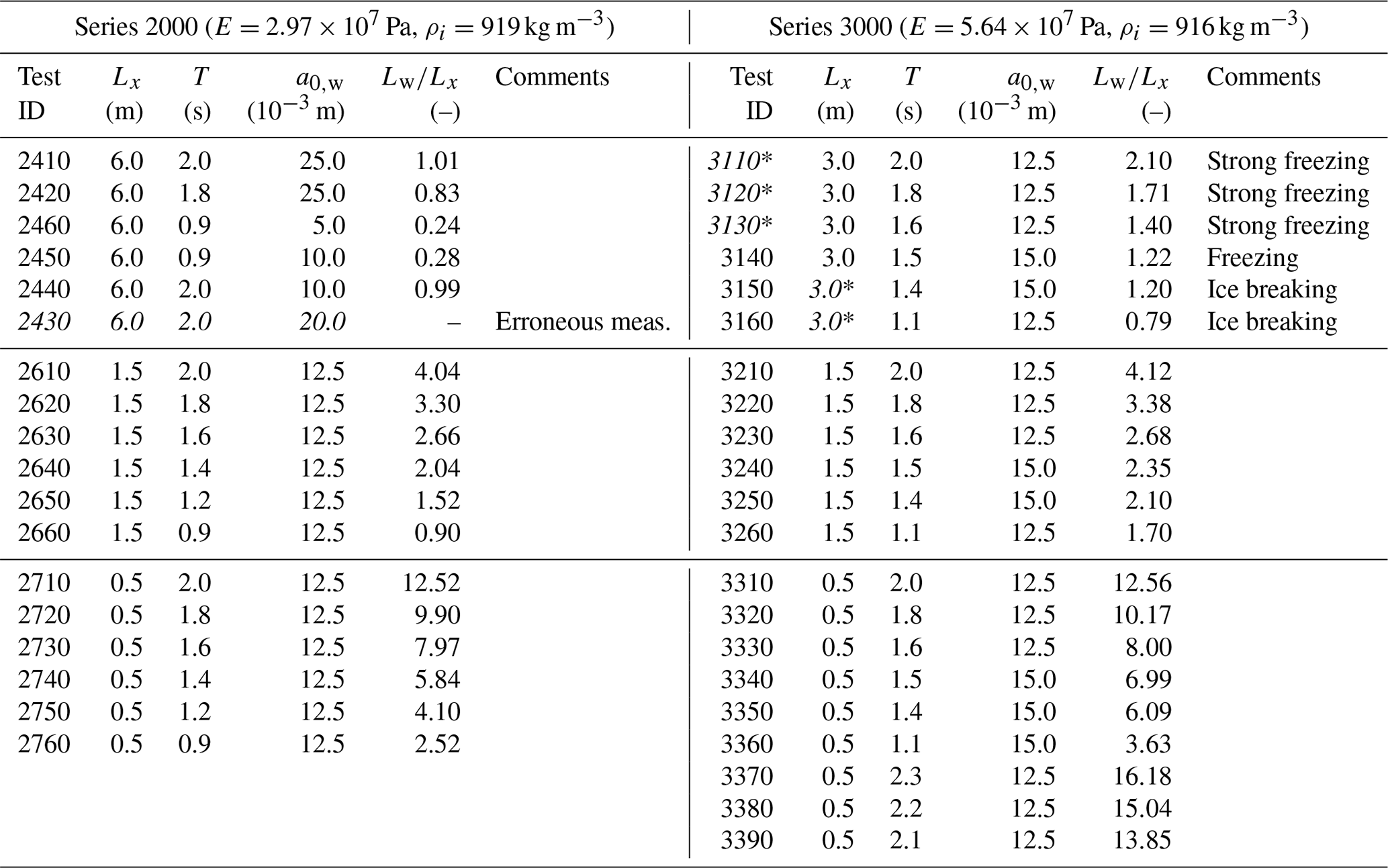
The air temperature during the tests was close to 0 ∘C; nevertheless, strong freezing was observed at the beginning of test series 3000 both between neighbouring ice floes and between the ice sheet and the side walls of the tank. As a result, the ice in tests 3110–3130 (and, to a lesser extent, in test 3140) behaved as a continuous sheet rather than separate floes, and the vertical ice deflection in the central part of the tank (rows 3 and 4) exceeded the incident wave amplitude, whereas it was close to zero along the walls (rows 1 and 6), making the results of those tests of little use from the point of view of this study. Moreover, strong breaking of ice floes occurred during the course of test 3150 (see Supplement Movie 1): in the central rows of floes (j=3 and j=4), the first four floes starting from the ice edge () broke within the first 15–20 s of the test; after roughly 1 min, the first two floes, initially 3 m long, were broken into four pieces each. Thus, the test 3150 and especially the subsequent test 3160 in fact represent cases with floes smaller than 3 m in the area within 12 m from the ice edge. Remarkably, also, as the Supplement Movie 1 clearly shows, slightly different timing of breaking in the two neighbouring rows of floes in the middle of the tank resulted in the visibly different intensity of overwash, with stronger overwash over smaller floes. This shows clearly how sensitive the behaviour of the wave–ice system is to seemingly slight changes of conditions. Overall, strong overwash was observed in several tests, especially those with short waves and thus relatively high wave steepness (although, due to stronger attenuation, the region with overwash was in those cases limited to a relatively narrow zone close to the ice edge). Further down the ice sheet, starting from 15–20 m from the edge, only weak overwash was present that did not cover the whole upper surface of the floes; on the contrary, it was limited to floes' boundaries and clearly related to closing of spaces between floes during collisions (Supplement Movie 2).
The wave amplitude data of interest in this study was obtained by two methods (Fig. 1): underwater pressure sensors mounted along the side wall of the tank and, in series 3000, by the Qualisys system, recording the three-dimensional position of markers placed on the ice. (In a few tests in series 3000, two inertial measurement units, or IMUs, were additionally used and placed on a row of floes neighbouring the Qualisys markers, as seen in Fig. 1 and Supplement Movie 1 and 2; however, as they essentially duplicate the information provided by Qualisys, we do not use them in our analysis.)
The pressure sensors were located at a depth of 0.35 m and distance 0.65 m from the walls. The 12 Qualisys markers were placed along the central axis of the tank (floe row j=4), between x=34.25 m and x=39.75 m, at a 0.5 m distance from each other, in such a way that in the last group of tests (3310–3390) one marker was located in the middle of each 0.5 m long floe (Fig. 1). Importantly, in order to eliminate contamination from waves reflected from the beach at the end of the tank, sufficiently short time series were used to determine the vertical deflection of the ice along the tank. All details of data processing can be found in Cheng et al. (2018) and will not be repeated here.
Figure 2 shows wavenumbers k determined from the pressure sensor data in both test series (see also Cheng et al., 2018). As can be seen, all values of k from the tests with the smallest floes, Lx=0.5 m (triangles in Fig. 2), lie within the region bounded by the curves corresponding to the mass loading dispersion relation (β2=0 in Eq. 1) and open-water dispersion relation (). In tests with larger floes, as can be expected, the wavenumbers are lower, with values between those computed from the elastic-plate and open-water models. The decrease in k with increasing Lx occurs in all cases except in test 3160, in which, as noted above, the actual floe size was smaller than 3 m due to ice breaking.
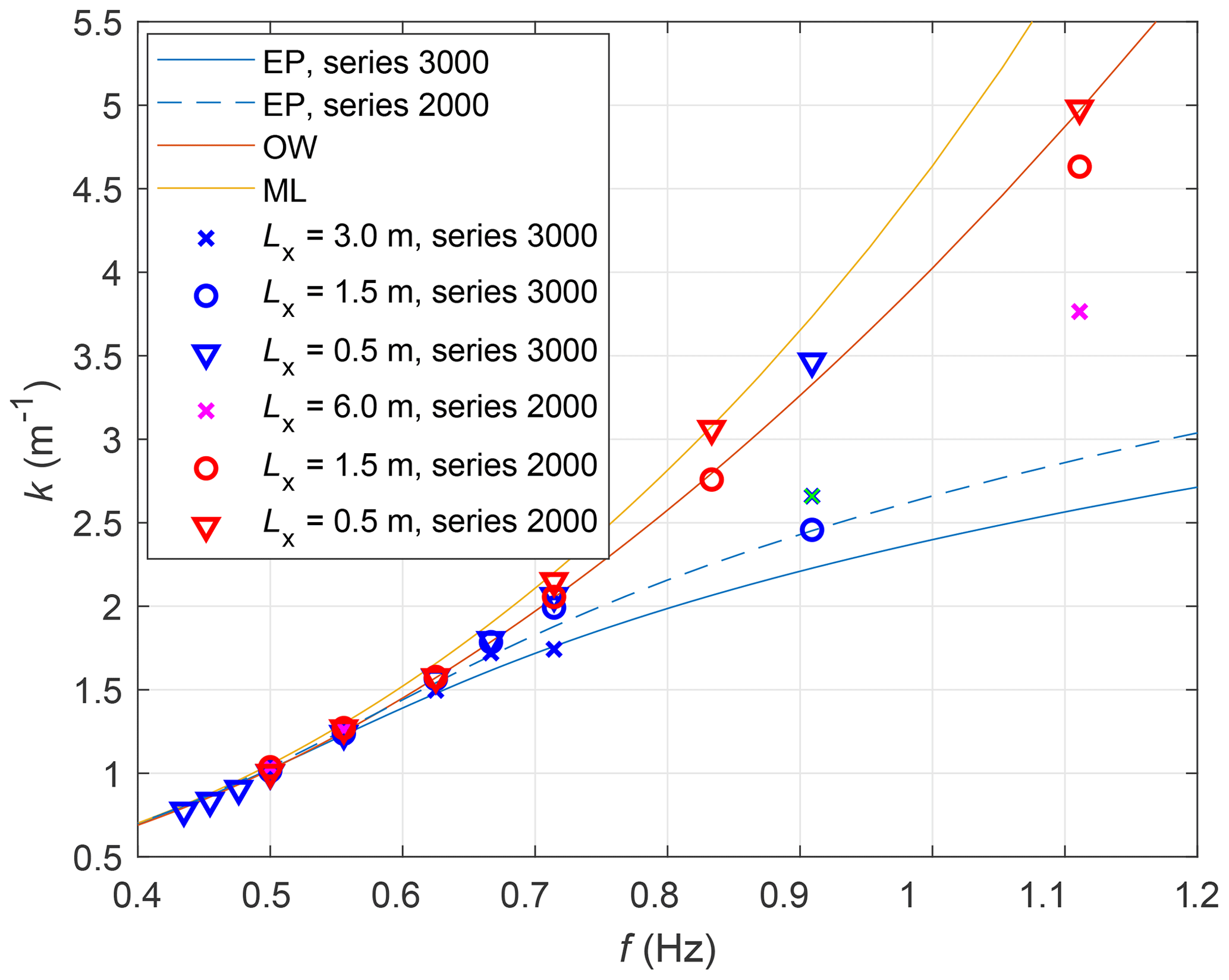
Figure 2Wavenumber k (m−1) in the experiments from LS-WICE series 2000 and 3000 together with corresponding wavenumbers from the elastic-plate (EP), open-water (OW), and mass loading (ML) dispersion relations (in the case of ML, the curves for both series are indistinguishable). The cross symbol shown in green corresponds to test 3160, nominally with Lx=3.0 m but with smaller actual floe size due to breaking. See Cheng et al. (2018) for more details.
3.2 Observed wave attenuation
In this section we analyse the wave attenuation observed in the LS-WICE experiments based on the data from pressure sensors and from the Qualisys system – two data sources that provide a slightly different picture of the situation due to the fact that the pressure sensors have fixed positions relative to the tank and the Qualisys markers have fixed positions relative to the ice. In order to better understand the observed attenuation patterns, we supplement the data analysis with vertical deflections computed from the MEEM model described in Sect. 2.1. The exact purpose of using MEEM was to estimate the contribution of scattering to the overall attenuation (in most tests expected to be small) and to identify those tests in which scattering did have dominant influence on attenuation so that they could be eliminated from the subsequent validation of the DEM (Sect. 4).
The amplitudes determined from measurements and computed with MEEM are shown in Supplement Figs. S1 and S2 and, for two selected tests, in Fig. 3. The first important observation from the amplitude profiles along the tank computed with MEEM is that – as expected – in the majority of tests, both the total amplitude aMEEM,tot and the amplitude of the transmitted propagating component remain fairly constant throughout the length of the tank, suggesting that the wave attenuation due to scattering is very limited (importantly, the results do not change significantly if small gaps between ice floes that are a few millimetres wide are included in the MEEM set-up, analogous to those present in the laboratory). The exceptions are tests 2640, 3110, and 3250, all three with floe length Lx being equal to almost exactly half of the wavelength (see Lw∕Lx ratios in Table 1), and, to a lesser extent, tests with the highest wave frequency, i.e. those with the lowest Lw∕Lx ratios. Also, for a given floe size, the ratio decreases with a decreasing wave period – the contribution of the damped travelling components, leading to stronger deflection of the edges of the floes, is more significant for short waves than for long waves. Those observations are summarized (for test group 3000) in Fig. 4. In spite of the fact that the amplitude decreases with increasing wave frequency (Fig. 4a), i.e. at high wave frequencies a substantial part of wave energy is contained within the damped components, in the majority of tests this energy redistribution does not lead to significant wave attenuation – the transmitted amplitude at the end of the tank is very close to the initial amplitude a0,w in all tests except those mentioned earlier (Fig. 4b). Importantly, also, although the redistribution of wave energy among the propagating and damped propagating components clearly depends on floe size, the amount of wave energy reaching the down-wave end of the tank is almost the same for all three floe sizes considered.
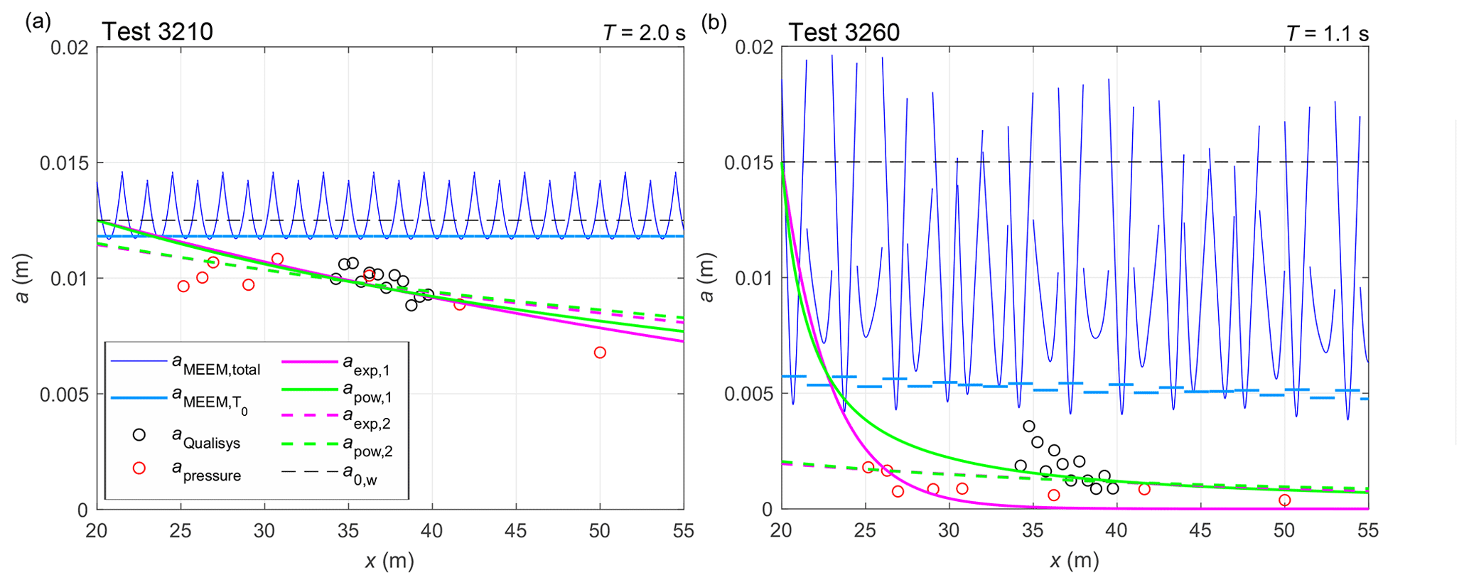
Figure 3Amplitude of the vertical ice deflection along the tank in two selected tests from series 3000: 3210 (a) and 3260 (b; for analogous plots for all tests from both series, 2000 and 3000, see Supplement Figs. S1 and S2). The measured amplitude is shown with red (pressure sensors) and black (Qualisys) circles. Thin blue lines show the total amplitude from the MEEM model; the corresponding amplitudes of the transmitted propagating mode (T0) are shown with thick light-blue lines. The black dashed line shows the wave-maker amplitude a0,w. Green and magenta lines are least-square fits of the data with Eq. (4) and Eq. (5), respectively (continuous lines: prescribed a0; dashed lines: fitted a0). See text for details.
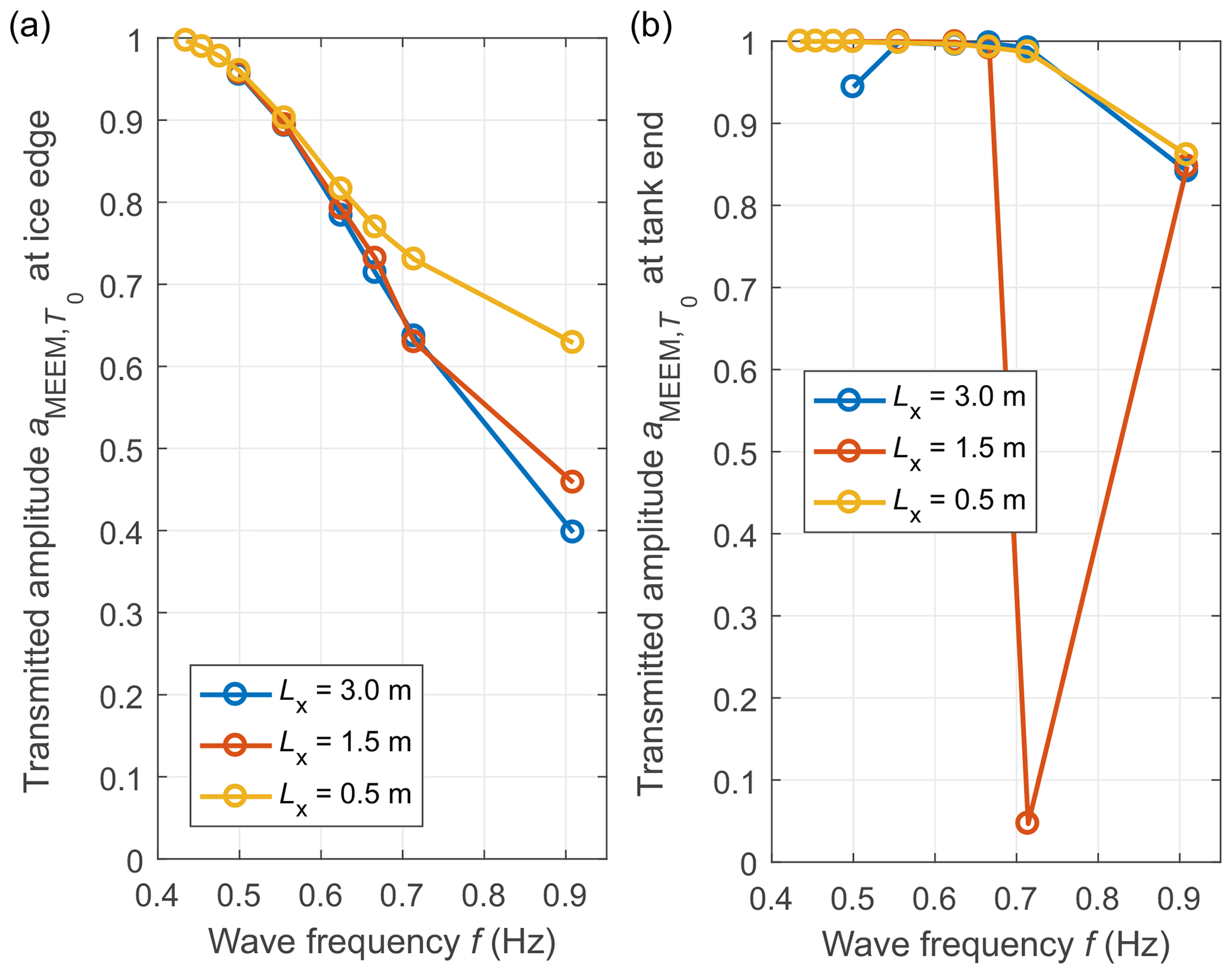
Figure 4Transmission coefficients computed with the MEEM model for tests from group 3000 (the results for group 2000 are similar): amplitude of the transmitted propagating component at the ice edge (a) and at the end of the tank (i.e. after propagating through the whole ice sheet; b). All amplitudes are normalized with the respective a0,w.
Within the ice-covered region, the redistribution of wave energy among different components means that large amplitude differences can be expected within a single floe, resulting not from the overall wave attenuation but from the contribution of multiple wave modes at each floe edge – and this effect becomes stronger with increasing floe size. Figure S3, showing zoomed fragments of the tank around the location of the Qualisys markers, provides a good illustration of that variability, present both in MEEM results and, to a lesser extent, in the measured data. In consequence, the vertical deflection of the ice measured at a single point is of little value, especially if the measurement is done at a fixed position in space (as is the case with the pressure sensors in our experiment), so that the location of the sensor relative to the floes' boundaries is unknown and might change slightly during a single test. In the case of Qualisys measurements, an attempt could be made to “split” the measured amplitudes among the transmitted propagating and remaining modes, based on the corresponding amplitudes from the MEEM model (aMEEM,tot and ), but this approach requires several rather arbitrary assumptions, including that about the same ratio in non-dissipative waves considered by MEEM and in dissipative waves observed in the tank. Without those assumptions, a way to proceed is to come to terms with the high scatter of the measured amplitudes (resulting from scattering processes as well as uncertainties related to measurement method and data processing) even though this means that the data provide useful information on attenuation only if, first, a large number of sensors are available and, second, if they are distributed over a long distance.
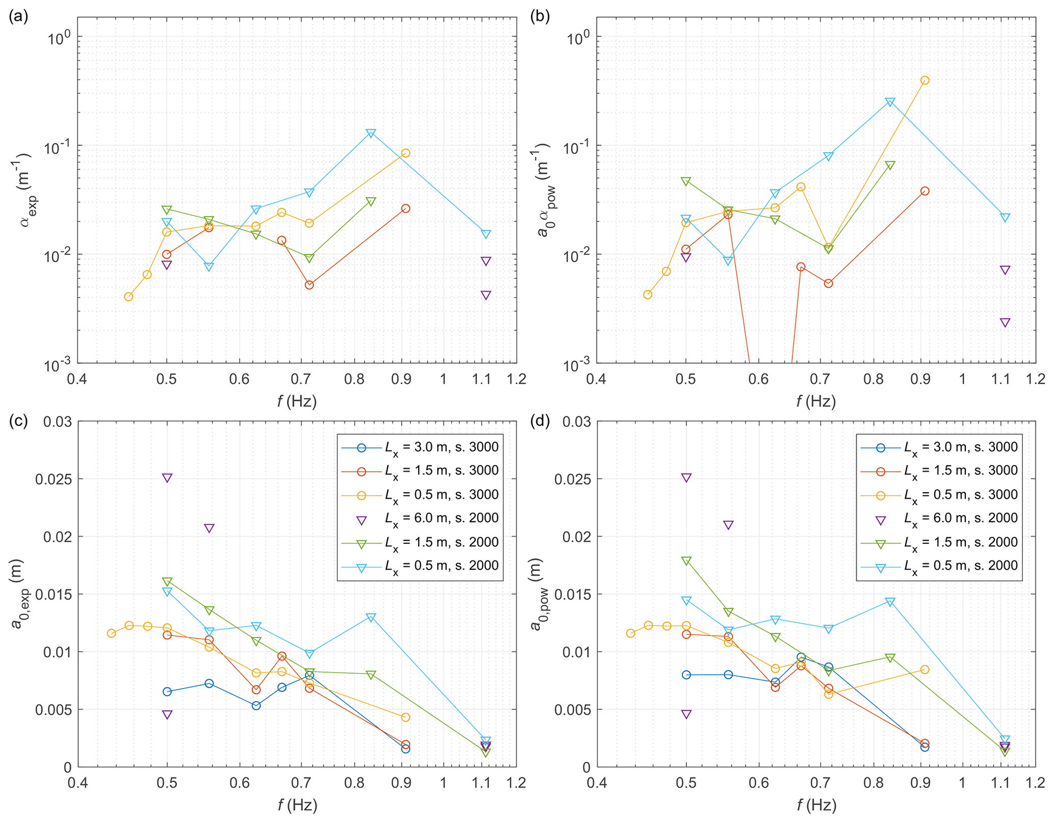
Figure 5Attenuation rates (m−1; a, b) and a0 (m; c, d) in function of wave frequency f (Hz) obtained by fitting Eq. (4) (a, c) and Eq. (5) (b, d) to the observed LS-WICE data, with a0 being treated as a fitted coefficient. Note that in some tests (e.g. series 3000 with Lx=3.0 m) the fitted values of α are negative and therefore are not shown in panels (a and b).
A cursory inspection of Figs. 3 and S1–S3 is enough to conclude that the MEEM model – that is, scattering alone – does not explain the variability in wave amplitudes observed in LS-WICE. Qualitatively, the measured values are, in most tests, well below those computed with MEEM, suggesting an important role of dissipative processes. Also, as can be expected, attenuation increases with increasing wave frequency – a very rough quantitative measure supporting this observation can be obtained by simply computing an average measured amplitude for each test (not shown). In order to gain more insight into the observed attenuation, we fit the data with two theoretical curves, the exponential function
and Eq. (3) predicted by the model of dissipation due to ice–water drag, derived in Part 1,
In Eqs. (4) and (5), denotes the distance from the ice edge, located at x=x0. Both fits are computed in two versions: the wave amplitude at the ice edge, a0, is treated either as a freely adjustable parameter (together with αexp or αpow, respectively) or is fixed to the value of the wave-maker amplitude a0,w used in a given test. In other words, in the first approach, a0 is assumed to be unknown and is part of the solution; the second approach might be viewed as analogous to a field case in which open-water, incident wave height is known, e.g. from a spectral wave model or satellite observations (as in, for example, Stopa et al., 2018a), and attenuation within the ice is expressed relative to those open-water conditions (which amounts to implicitly assuming negligible reflection at the ice edge). Notably, the exponential fit with adjustable a0 was applied to LS-WICE data by Cheng et al. (2018), who concluded based on the results that there was no dependence of the attenuation rate on wave frequency. Indeed, treating a0 as a free parameter produces fits with αexp and αpow very strongly (and apparently randomly) varying from test to test (Fig. 5a, b) and with a0 values that simply reflect the above-mentioned decrease in the area-averaged amplitude with frequency (Fig. 5c, d; it is also worth noting that in some tests fitting the data with a constant produces fits with better quality than either Eq. 4 or Eq. 5). Accordingly, the fitted a0 is in most cases much lower than both a0,w and aMEEM,tot and even than the transmitted component ; in some tests (e.g. 3160 or 3360) the difference exceeds 50 %. Notably, also, in a few tests the fitted attenuation rates are negative.
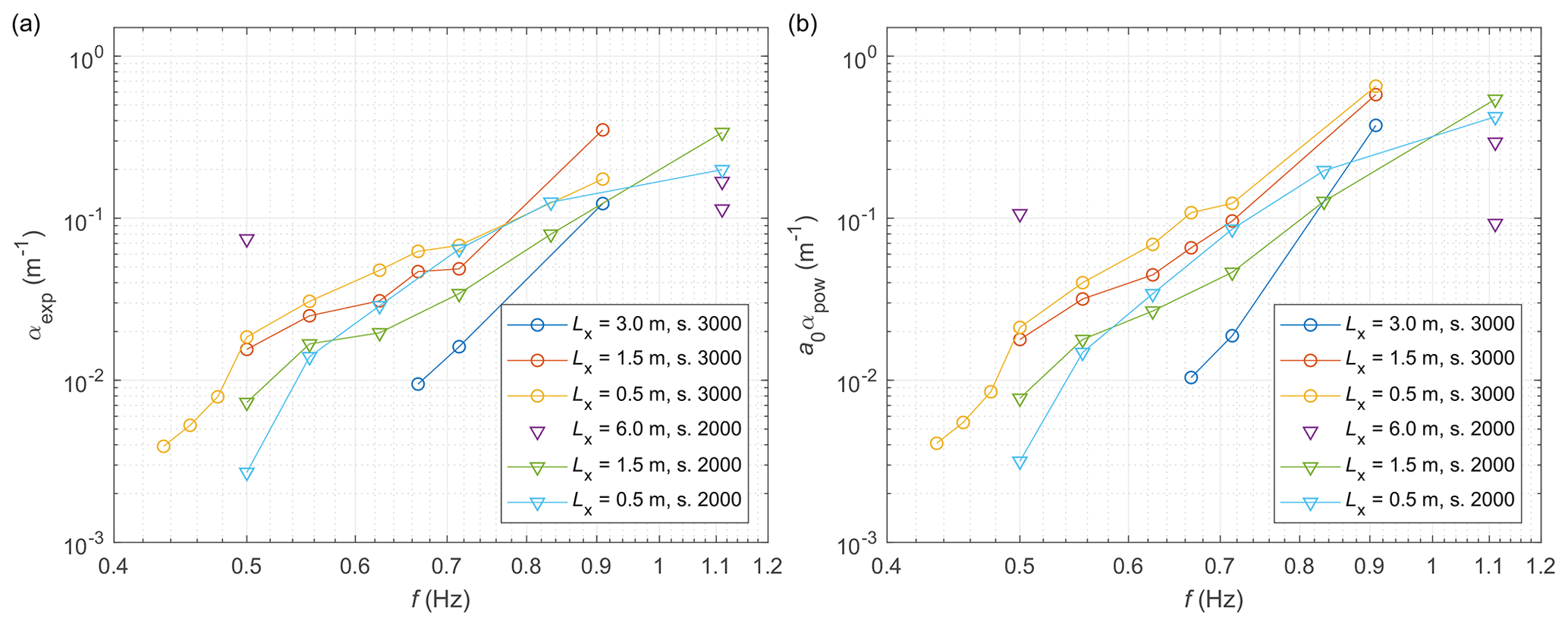
Conceptually speaking, because the attenuation takes place within the ice cover, the wave amplitude at x0 should be the amplitude that the actual wave transmits into the leading ice edge, which might be very different from a0,w. However, in the case of LS-WICE, due to limited reflection at the ice edge, fixing the values of a0 at the respective a0,w produces very regular results (Fig. 6), with consistent variability in α(f), even though, understandably, the goodness-of-fit measures become slightly worse (one free parameter instead of two). Several of the curves in Fig. 6 can be approximated with (for both attenuation models), but the power nα is extremely sensitive to individual data points (for example, removal of a single point, corresponding to the highest wave frequency, from the data from series 3200 changes nα from 7 to 3.1), making any quantitative inferences regarding α(f) of little value.
The very different results obtained with fixed and fitted a0 values can be to a large degree attributed to the fact that no data points are available within the first 5 m from the ice edge. The attenuation within the region where the sensors were located was small, but the amplitudes in that region were, on average, much lower than the forcing amplitude a0,w. Those differences, as the MEEM results indicate, cannot be explained by a reflection of wave energy from the ice edge. Thus, unless significant reflection took place at the floating boom, obviously not taken into account by the MEEM model, very strong attenuation must have taken place within the narrow zone between the ice edge and the first pressure sensors. We return to this issue further in Sect. 4 in the context of the results of numerical simulations. Here, it is worth stressing that – whatever the reasons for large amplitude differences between the wave maker and the inner parts of the ice sheet – the fits with adjustable a0 values should be treated as suitable for that inner zone only and should not be extrapolated to the region close to the ice edge. It should be also remembered that, due to limited number of data points and high spatial variability in wave amplitude related to the bending of the floes, discussed above, the fitted values of αexp and αpow are extremely sensitive to individual data points. On the other hand, the fits with a fixed a0 by construction better represent relationships between the forcing wave amplitude and that within the ice at the cost of worse agreement with the data within the inner zone of low attenuation.
Finally, it is worth noting that the available data do not provide arguments in favour of any of the two fit types considered. Especially when a0 is treated as an adjustable parameter, the two fitted curves, Eqs. (4) and (5), are in many tests almost undistinguishable (Figs. S1 and S2). Although one function might better represent the data than the other for a particular test, the goodness-of-fit measures calculated globally for all tests are almost identical for both fitting functions. For example, in the version with fitted a0, the standard deviation of differences between the observed and fitted amplitudes (scaled with the respective a0,w) equals 0.0618 for Eq. (4) and 0.0624 for Eq. (5). When a0 is fixed, the corresponding values are 0.0875 and 0.0714, respectively. The bias is in all cases below 10−2, negative with fitted a0, and positive with fixed a0. In spite of those similarities, however, with fixed a0 values, the fit (Eq. 5) predicts stronger attenuation close to the ice edge and weaker attenuation further down-wave (where, for small wave periods, e.g. in tests 3160, 3260, 3360, the exponential fit gives displacement close to zero).
3.3 A note on scaling
Although extrapolation of any quantitative data from the laboratory scale to the field scale has to be approached with caution, it is useful – before proceeding to the analysis of the modelling results – to relate the range of ice and wave parameters used in the experiment to the analogous full-scale conditions.
For an unscaled ice thickness of, say, 1.5 m, typical for first-year ice in many regions of the Arctic and Antarctic, and the laboratory ice thickness is hi=0.036 m, the scaling factor is s≈40, giving an unscaled water depth slightly larger than 100 m. Based on hi and the measured wavenumbers (Table 1 and Fig. 2), the values of khi varied between 0.036 and 0.179 in test group 2000 and between 0.028 and 0.125 in test group 3000. For the assumed unscaled ice thickness, this corresponds to unscaled wavelengths in the range 50–260 m and 75–337 m, respectively, i.e. wave periods of 5.8–13 s and 7–15 s. The unscaled open-water wave amplitudes varied between 0.2 and 1.1 m. Thus, in both groups of tests, the wave forcing used in the laboratory corresponds to realistic wave conditions in the marginal ice zone. The range of floe sizes used in the laboratory corresponds to the field-scale size range of 21–250 m. The ratio of the elasticity length scale to the ice thickness hi in the laboratory equals 9.6 and 11.2 (for test groups 2000 and 3000, respectively). With the unscaled ice thickness assumed above, and with elastic modulus of 109 Pa, typical for sea ice, the corresponding ratio is 9.12; i.e. it is comparable to the scaled one.
Crucially, the observed attenuation rates are realistic as well, although they tend to lie within the upper range of observed ones. For example, Stopa et al. (2018b), in their extensive analysis of over 2000 situations of swell propagation in sea ice, obtained attenuation rates from 10−6 m−1 to over 10−3 m−1, with the majority of values between 10−5 m−1 and 10−4 m−1. For the range of wavelengths over which the two studies (Stopa et al., 2018b, and the present analysis) overlap, i.e. between 100 and 350 m, the unscaled values of attenuation in LS-WICE are – m−1 (corresponding to laboratory values of αexp and a0αpow, shown in Fig. 6 for frequencies below 0.75 Hz). For the shortest waves analysed in LS-WICE, the unscaled attenuation rates are higher, even as high as 10−2 m−1, but, as attenuation of waves with periods of 6–7 s and lengths much lower than 100 m is rarely studied in the field, it is difficult to assess whether these values should be regarded as exceptionally high.
In Part 1, the coupled DEM–wave model was set up with sea ice properties corresponding to those from LS-WICE series 3000, and the model sensitivity was analysed within a multi-dimensional parameter space. Here, we run the model for each test from series 3000, with floe length Lx, wave period T, and incident wave amplitude a0,w used in that test (Table 1). The average floe–floe distance df is very difficult to determine accurately. We fixed df at m, which is a value from the set of values tested in Part 1 that we find to be appropriate based on visual observations of the ice; undoubtedly, df belongs to the model parameters with high uncertainty. As the group velocity is not available from observations but necessary to solve the wave energy transport equation, the open-water dispersion relation was assumed to be suitable for tests with Lx=0.5 m and the elastic-plate dispersion relation for tests with longer floes (see Fig. 2; note that significant differences between cg values computed from those two models are present only for the two highest wave frequencies considered).
With the basic settings listed above, the model was run several times for each test, with different combinations of the following four parameters: drag coefficient Csd, restitution coefficient ε, and the coefficients smin and cow used in Eq. (2) to calculate the overwash thickness. The goal of the simulations was to find combinations of those parameters that optimally reproduce the observational data over the available range of floe sizes and wave frequencies. This is equivalent with an assumption that – as the general conditions and ice properties were stable throughout the whole test series 3000 – the same set of parameters should be suitable for reproducing wave attenuation in all tests. In other words, in the absence of evidence to the contrary, we disregard the possible dependence of Csd, ε, etc., on wave period and amplitude.
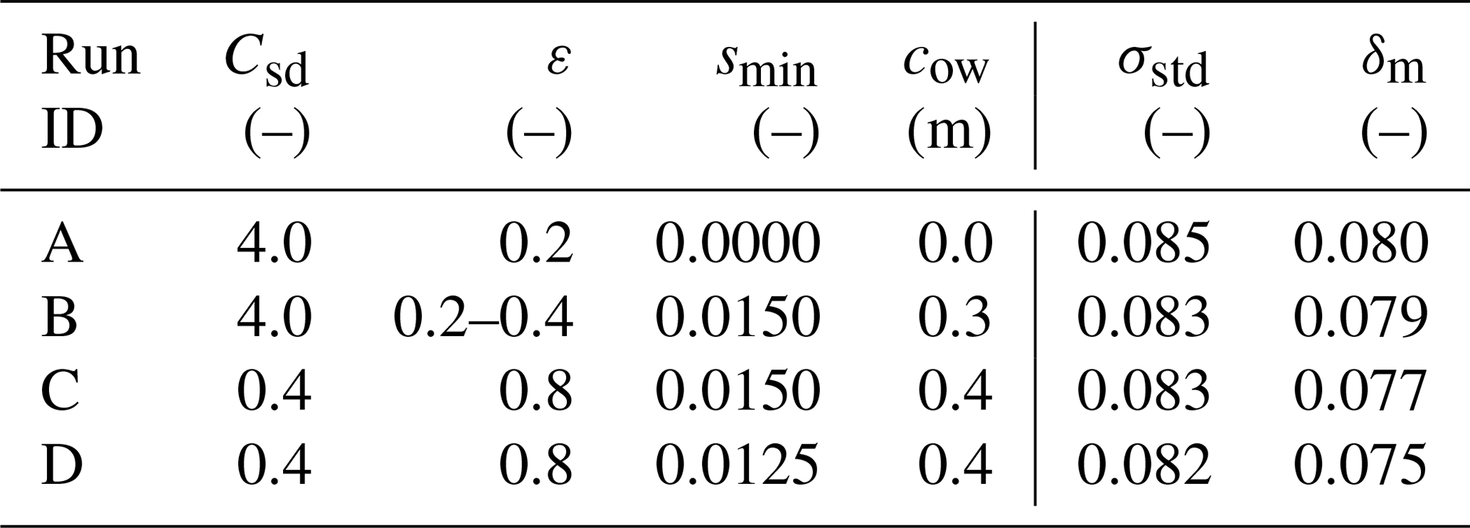
Before we proceed to the analysis of the DEM simulations, it is worthwhile to note that the suitable values of Csd can be constrained from observational data and from the results of the theoretical analysis in Part 1. Due to the lack of observational points close to the ice edge, it is reasonable to assume that the measurements represent the inner “regime”, for which the attenuation rates αpow are related to Csd by Eq. (3). As already discussed in the previous section, the values αpow obtained by fitting with variable a0 (more suitable for the inner zone than fitting with fixed a0) vary strongly from test to test; however, for test series 3300 (yellow line in Fig. 5b), αpow can be robustly fitted with Eq. (3), assuming an open-water dispersion relation and deep water, i.e. . The resulting value of Csd is very high and equals 4.04. More generally, in order to obtain attenuation rates in the observed range of 10−2–10−1 m−1 within the frequency range considered, values of Csd between 10−2 and 101 are necessary. We leave the discussion of how realistic those values are for the next section. Here, we concentrate on analysing the combinations of Csd, ε, smin, and cow that produce results in good agreement with observational data. Two quantities are used as a measure of the model performance; these are the standard deviation of differences σstd and mean difference (bias) δm between the modelled and observed normalized amplitudes from 14 tests: 3210–3240, 3260, and all nine tests from series 3300. Tests 3250 and 3140–3160 are included in the computations but excluded from validation due to the very strong influence of scattering-induced attenuation (3250) and due to problems with freezing and ice breaking (series 3100; see Sect. 3). The model set-ups considered to be satisfactory according to the above criteria, numbered from A to D, are summarized in Table 2. Figure 7 shows the simulated amplitude profiles along the tank for two selected tests; analogous plots for all tests can be found in Fig. S4. Overall, in set-ups with no or weak overwash (i.e. high smin and low cow), both the bias and standard deviation of differences increase with increasing ε, making only set-ups with the lowest ε tested (0.2) satisfactory. On the other hand, set-ups with strong overwash and smaller ice–water drag show an opposite behaviour, with relatively stable σstd for all values of ε but with bias decreasing with increasing ε.
Table 2Adjustable parameters of the model set-ups discussed in Sect. 4 and the corresponding statistical measures of the model performance.
In the case of set-up B, two values of ε, 0.2 and 0.4, gave almost identical results in terms of both σstd and δm.
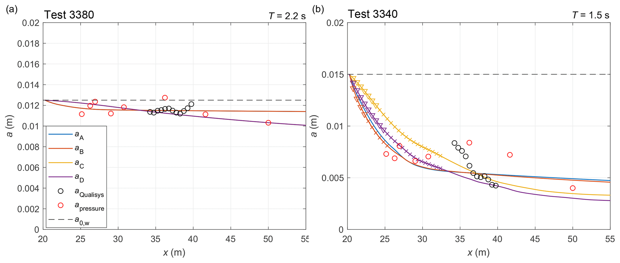
Figure 7Amplitude of the vertical ice deflection along the tank in two selected tests from series 3000: 3380 (a) and 3340 (b; for analogous plots for all tests from series 3000, see Fig. S4). The measured amplitude is shown with red (pressure sensors) and black (Qualisys) circles. The black dashed lines show the wave-maker amplitude a0,w. The remaining lines show DEM results obtained with set-ups A–D (see Table 2). Locations with overwash are marked with crosses, and those where the change of wave amplitude due to overwash from one floe to the next exceeds 1 mm are marked with triangles.
As expected from the analysis above, simulations without overwash require very high values of Csd, and the optimal configuration is obtained for Csd=4.0 (the neighbouring values tested equaled 3.0 and 5.0) and ε=0.2 (set-up A). Very similar values of σstd and δm are obtained with cow=0.3 (set-up B) – interestingly, the results of runs A and B are very close in terms of wave amplitudes in the region where the sensors were located; they mostly differ from each other in the area close to the ice edge in tests with short, and thus steep, waves (e.g. test 3360). In those tests, overwash contributes significantly to attenuation within the first few metres of the ice in set-up B, and it is not present (by definition) in set-up A. This means that in the two set-ups, A and B, different processes contribute to wave dissipation at the ice edge, but their net effect further down-wave is similar: dissipation due to overwash in B leads to a faster initial decrease in wave amplitudes, but the zone of strong dissipation becomes narrower. Notably, as far as we can judge from a visual analysis of the video material, set-up B produces realistic results in terms of the extent of the overwash regions for different wave periods. However, with no sensors located close to the ice edge, it is not possible to identify set-up B as “better” than A based on the statistics in Table 2.
The extent of overwash is, as expected, larger in runs C and D, and in some tests the model predicts overwash over the entire ice sheet – which was not observed; but, before labelling those set-ups as unrealistic, it is worth noting that the simulated dissipation due to overwash was in those cases extremely small over most of the area far from the ice edge. As can be seen from Fig. 7 and Fig. S4, in spite of very similar σstd and δm, the slope of the wave amplitude curves in set-ups C and D is very different from that in set-ups A and B – and, although Csd is in C and D an order of magnitude smaller than in A and B, the slope is higher in the first case. Whereas set-ups A and B tend to underestimate wave amplitudes at the ice edge and to overestimate them in the down-wave region, set-ups C and D exhibit an opposite tendency. As said, this results in similar overall performance, although, obviously, some set-ups perform clearly better than others for individual tests.
In summary, it should be stressed that the values of σstd in all four set-ups are comparable with analogous statistics for the least-square fits described in the previous section – in spite of the fact that parameters of each fit were optimized to the individual test. In view of that, it is remarkable how well the same set of model parameters reproduces the observed variability in wave amplitudes over all tests considered.
The LS-WICE results analysed in this work provide a very good example of how difficult it is to quantitatively assess wave energy attenuation in sea ice (especially in laboratory conditions, with a limited number of floes and over short distances) and to attribute the observed attenuation to individual physical processes even in a highly idealized laboratory setting. In spite of the simple geometry, regular wave forcing with small wave amplitudes, and highly uniform ice properties, several processes simultaneously modify wave propagation and dissipation, including floe collisions, floe breaking, overwash of the ice surface, production of slush, freezing between neighbouring floes and between the ice and tank walls, and possibly some others. The results of observations and of the MEEM model clearly show that the scattering model alone does not explain the observed spatial variability in wave amplitudes in fragmented ice, as the attenuation simulated with MEEM is, in most tests, very low – much lower than the observed one. Another general conclusion drawn from the data analysis is that the attenuation rates increase with increasing wave frequency. The two facts together mean that the patterns of wave attenuation observed in LS-WICE are predominantly shaped by dissipative processes and that the effectiveness of those processes in attenuating wave energy is frequency dependent.
An important aspect of the numerical part of this study is that several different combinations of the model parameters lead to reasonable agreement with observational data – even though we limited the number of adjustable parameters to three. It is very likely that even more regions of good model performance could be found within a higher-dimensional parameter space. Obviously, this ambiguity is a consequence of a large number of poorly constrained coefficients, large uncertainties in measured data, and the fact that the vertical deflection of the ice, being a combined effect of many processes, is the only validated quantity. Although some combinations of the parameters seem more “realistic” than others, it is hard to favour one set-up against the other without additional data. In particular, very high values of the drag coefficient in our “successful” set-ups are a few orders of magnitude higher than those reported in the literature, which are rarely larger than 10−2 (Castellani et al., 2018). The fact that the DEM reproduces the observed attenuation with such high drag coefficients indicates that, whatever the dissipative processes actually contributing to attenuation were, they can be described mathematically with formulae similar to those used to compute skin drag in our model. In other words, this indicates that forces contributing to dissipation in LS-WICE were approximately proportional to the under-ice orbital velocities squared, and Csd can be treated as an effective drag coefficient rather than a skin drag coefficient. Notably, very similar formulae to those underlying our model were used in a recent study by Voermans et al. (2019) to quantify turbulent kinetic energy dissipation rates under sea ice, with a result suggesting a rapid increase in the effective drag with increasing ice concentration. Although one should be extremely careful with extrapolating data from lower ice concentrations (up to 0.8 in Voermans et al., 2019) to compact ice (close to 1 in our study), effective drag of the order of 1 seems plausible. In any case, in all our simulations with reasonable results, the necessary values of Csd were higher than 0.1 unless extremely low smin and high cow were used, producing strong overwash over much of the ice surface even in tests with long waves – which was not what was observed in the laboratory.
Undoubtedly, from the point of view of analysing wave attenuation, a number of shortcomings can be listed in the LS-WICE set-up, and, based on this study, several recommendations can be formulated for future laboratory experiments designed specifically for measuring wave attenuation in fragmented sea ice (and, more generally, in other types of floating ice as well). First of all, it is crucial to locate sensors measuring the vertical deflection of the ice, acceleration of ice floes, and possibly other quantities, in the zone of the strongest attenuation close to the ice edge. At the same time, it is important not to limit the observations to that zone, as the attenuation further down-wave is very likely much weaker and cannot be extrapolated from that observed at the ice edge. Moreover, distributing sensors over a possibly large distance is necessary if the suitability of alternative theoretical attenuation curves is to be tested. The LS-WICE data, as demonstrated in this work, are clearly not sufficient for that purpose. It must be remembered, however, that this requirement is easy to formulate but very hard to fulfil in a wave tank, as its length limits the possible number of wavelengths. Furthermore, as discussed at the beginning of this section, LS-WICE shows that, although it would be desirable to design experiments eliminating all other dissipation mechanisms except the one of interest, this goal is very hard, if not impossible, to achieve. Some factors present in LS-WICE, e.g. freezing to the side walls, can be eliminated with some effort (though it is not straightforward in an ice tank several tens of metres long), but the influence of other factors has to be accepted and, as they are impossible to eliminate, quantified. In particular, overwash is very difficult to eliminate in laboratory conditions due to small thickness and therefore very low freeboard of the ice so that, apart from recording overwash presence and extent by video, assessment of its thickness is desirable, enabling formulation of more advanced parameterizations than the primitive one proposed in this study.
Finally, as already mentioned in the discussion in Part 1, integrating scattering effects in the DEM presented here is a major challenge that must be addressed to make the model suitable for analysing mutual relationships between non-dissipative and dissipative processes contributing to wave energy attenuation. Obviously, attenuation in real sea ice is not a simple superposition of individual processes that can be considered independently of each other, as in the present study.
The code of the DESIgn model is freely available at https://herman.ocean.ug.edu.pl/LIGGGHTSseaice.html (Herman, 2019) and as a Supplement to Herman (2016). The extended code necessary to reproduce the results presented in this paper, together with input scripts, can be obtained from the corresponding author. The LS-WICE data used in this paper are described in the data storage report available at https://zenodo.org/record/1067170 (Tsarau, 2016) and can be obtained from the authors.
The supplement related to this article is available online at: https://doi.org/10.5194/tc-13-2901-2019-supplement.
All authors contributed to planning of the research and to the discussion and analysis of the results. SC performed the analysis of experimental data and the MEEM simulations. AH performed the numerical simulations and wrote the text.
The authors declare that they have no conflict of interest.
The authors would like to thank the Hamburg Ship Model Basin (HSVA), especially the ice tank crew, for the hospitality, technical and scientific support, and the professional execution of the test programme in the research infrastructure ARCTECLAB. We are also very grateful to two anonymous reviewers for very insightful and constructive comments on the draft of this paper.
The development of the numerical model used in this work has been financed by the Polish National Science Centre research grant no. 2015/19/B/ST10/01568 (“Discrete-element sea ice modeling – development of theoretical and numerical methods”). The co-authors Sukun Cheng and Hayley H. Shen are supported in part by ONR grant no. N00014-17-1-2862. The laboratory work described in this publication was supported by the European Community’s Horizon 2020 programme through the grant to the budget of the Integrated Infrastructure Initiative Hydralab+, contract no. 654110.
This paper was edited by Lars Kaleschke and reviewed by two anonymous referees.
Castellani, G., Losch, M., Ungermann, M., and Gerdes, R.: Sea-ice drag as a function of deformation and ice cover: Effects on simulated sea ice and ocean circulation in the Arctic, Ocean Model., 128, 48–66, https://doi.org/10.1016/j.ocemod.2018.06.002, 2018. a
Cheng, S., Tsarau, A., Li, H., Herman, A., Evers, K.-U., and Shen, H.: Loads on Structure and Waves in Ice (LS-WICE) project, Part 1: Wave attenuation and dispersion in broken ice fields, in: Proc. 24th Int. Conf. on Port and Ocean Engineering under Arctic Conditions (POAC), 11–16 June 2017, Busan, Korea, 2017. a
Cheng, S., Tsarau, A., Evers, K.-U., and Shen, H.: Floe size effect on gravity wave propagation through ice covers, J. Geophys. Res., 124, 320–334, https://doi.org/10.1029/2018JC014094, 2018. a, b, c, d, e, f
De Santi, F., De Carolis, G., Olla, P., Doble, M., Cheng, S., Shen, H., Wadhams, P., and Thomson, J.: On the Ocean wave attenuation rate in grease-pancake ice, a comparison of viscous layer propagation models with field data, J. Geophys. Res., 123, 5933–5948, https://doi.org/10.1029/2018JC013865, 2018. a
Frankenstein, S. and Shen, H.: The effect of waves on pancake ice collisions, in: Proc. 3rd Int. Offshore and Polar Engng Conf., 6–11 June 1993, Singapore, 1993. a
Herman, A.: Discrete-Element bonded-particle Sea Ice model DESIgn, version 1.3a – model description and implementation, Geosci. Model Dev., 9, 1219–1241, https://doi.org/10.5194/gmd-9-1219-2016, 2016. a, b
Herman, A.: Wave-induced surge motion and collisions of sea ice floes: finite-floe-fize effects, J. Geophys. Res., 123, 7472–7494, https://doi.org/10.1029/2018JC014500, 2018. a, b
Herman, A.: DESIgn – Discrete-Element bonded-particle Sea Ice model, available at: https://herman.ocean.ug.edu.pl/LIGGGHTSseaice.html, last access: 7 November 2019. a
Herman, A., Tsarau, A., Evers, K.-U., Li, H., and Shen, H.: Loads on Structure and Waves in Ice (LS-WICE) project, Part 2: Sea ice breaking by waves, in: Proc. 24th Int. Conf. on Port and Ocean Engineering under Arctic Conditions (POAC), 11–16 June 2017, Busan, Korea, available at: http://www.poac.com/Papers/2017/pdf/POAC17_051_Agnieszka.pdf (last access: 7 November 2019), 2017. a
Herman, A., Evers, K.-U., and Reimer, N.: Floe-size distributions in laboratory ice broken by waves, The Cryosphere, 12, 685–699, https://doi.org/10.5194/tc-12-685-2018, 2018. a
Herman, A., Cheng, S., and Shen, H. H.: Wave energy attenuation in fields of colliding ice floes – Part 1: Discrete-element modelling of dissipation due to ice–water drag, The Cryosphere, 13, 2887–2900, https://doi.org/10.5194/tc-13-2887-2019, 2019. a
Hibler III, W. and Leppäranta, M.: MIZEX 83 mesoscale sea ice dynamics: Initial analysis, MIZEX Bulletin III, USACREL Special Report 84-28, 19–28, 1984. a
Hopkins, M. and Shen, H.: Simulation of pancake-ice dynamics in a wave field, Ann. Glaciol., 33, 355–360, 2001. a
Kohout, A.: Water wave scattering by floating elastic plates with application to sea-ice, PhD thesis, Univ. of Auckland, New Zealand, 188 pp., 2008. a, b
Kohout, A. and Meylan, M.: An elastic plate model for wave attenuation and ice floe breaking in the marginal ice zone, J. Geophys. Res., 113, C09016, https://doi.org/10.1029/2007JC004434, 2008. a
Kohout, A., Meylan, M., Sakai, S., Hanai, K., Leman, P., and Brossard, D.: Linear water wave propagation through multiple floating elastic plates of variable properties, J. Fluids Structures, 23, 649–663, https://doi.org/10.1016/j.jfluidstructs.2006.10.012, 2007. a, b, c, d
Kohout, A., Meylan, M., and Plew, D.: Wave attenuation in a marginal ice zone due to the bottom roughness of ice floes, Ann. Glaciol., 52, 118–122, 2011. a
Li, H. and Lubbad, R.: Laboratory study of ice floes collisions under wave action, in: Proc. 28th Int. Ocean and Polar Engng Conf. ISOPE-2018, sapporo, Japan, 10–15 June 2018, 2018. a, b, c
Lu, Q., Larsen, J., and Tryde, P.: On the role of ice interaction due to floe collisions in marginal ice zone dynamics, J. Geophys. Res., 94, 14525–14537, 1989. a
Martin, S. and Becker, P.: High-frequency ice floe collisions in the Greenland Sea during the 1984 Marginal Ice Zone Experiment, J. Geophys. Res., 92, 7071–7084, 1987. a
Martin, S. and Becker, P.: Ice floe collisions and their relation to ice deformation in the Bering Sea during February 1983, J. Geophys. Res., 93, 1303–1315, https://doi.org/10.1029/JC093iC02p01303, 1988. a
Martin, S. and Drucker, R.: Observations of short-period ice floe accelerations during leg II of the Polarbjørn drift, J. Geophys. Res., 96, 10567–10580, https://doi.org/10.1029/91JC00785, 1991. a
McKenna, R. and Crocker, G.: Ice-floe collisions interpreted from acceleration data during LIMEX'89, Atmos. Ocean, 30, 246–269, https://doi.org/10.1080/07055900.1992.9649440, 1992. a
Rabault, J., Sutherland, G., Jensen, A., Christensen, K., and Marchenko, A.: Experiments on wave propagation in grease ice: combined wave gauges and particle image velocimetry measurements, J. Fluid Mech., 864, 876–898, https://doi.org/10.1017/jfm.2019.16, 2019. a
Rogers, W., Thomson, J., Shen, H., Doble, M., Wadhams, P., and Cheng, S.: Dissipation of wind waves by pancake and frazil ice in the autumn Beaufort Sea, J. Geophys. Res., 121, 7991–8007, https://doi.org/10.1002/2016JC012251, 2016. a
Rottier, P.: Floe pair interaction event rates in the marginal ice zone, J. Geophys. Res., 97, C6, 9391–9400, https://doi.org/10.1029/92JC00152, 1992. a
Shen, H. and Ackley, S.: A one-dimensional model for wave-induced ice-floe collisions, Ann. Glaciol., 15, 87–95, 1991. a
Shen, H. and Squire, V.: Wave damping in compact pancake ice fields due to interactions between pancakes, in: Antarctic Sea Ice: Physical Processes, Interactions and Variability, 74, 325–341, 1998. a, b
Shen, H., Hibler III, W., and Leppäranta, M.: On the rheology of a broken ice field due to floe collision, MIZEX Bulletin III, USACREL Special Report 84-28, 29–34, 1984. a
Shen, H., Hibler III, W., and Leppäranta, M.: On applying granular flow theory to a deforming broken ice field, Acta Mech., 63, 143–160, 1986. a
Shen, H., Hibler III, W., and Leppäranta, M.: The role of floe collisions in sea ice rheology, J. Geophys. Res., 92, 7085–7096, 1987. a
Skene, D., Bennetts, L., Wright, M., and Meylan, M.: Water wave overwash of a step, J. Fluid Mech., 839, 293–312, https://doi.org/10.1017/jfm.2017.857, 2018. a
Stopa, J., Ardhuin, F., Thomson, J., Smith, M., Kohout, A., Doble, M., and Wadhams, P.: Wave attenuation through an Arctic marginal ice zone on 12 October 2015. 1. Measurement of wave spectra and ice features from Sentinel 1A, J. Geophys. Res., 123, https://doi.org/10.1029/2018JC013791, 2018a. a
Stopa, J., Sutherland, P., and Ardhuin, F.: Strong and highly variable push of ocean waves on Southern Ocean sea ice, P. Natl. Acad. Sci. USA, 115, 5861–5865, https://doi.org/10.1073/pnas.1802011115, 2018b. a, b
Tsarau, A.: Experimental study on wave propagation in ice and the combined action of waves and ice on structures – Data storage report, available at: https://zenodo.org/record/1067170 (last access: 7 November 2019), 2016. a
Voermans, J., Babanin, A., Thomson, J., Smith, M., and Shen, H.: Wave attenuation by sea ice turbulence, Geophys. Res. Lett., 46, 6796–6803, https://doi.org/10.1029/2019GL082945, 2019. a, b, c
Yiew, L., Bennetts, L., Meylan, M., Thomas, G., and French, B.: Wave-induced collisions of thin floating disks, Phys. Fluids, 29, 127102, https://doi.org/10.1063/1.5003310, 2017. a
Yiew, L., Parra, S., Wang, D., Sree, D., Babanin, A., and Law, A.-K.: Wave attenuation and dispersion due to floating ice covers, Appl. Ocean Res., 87, 256–263, https://doi.org/10.1016/j.apor.2019.04.006, 2019. a, b
Zhao, X. and Shen, H.: Wave propagation in frazil/pancake, pancake, and fragmented ice covers, Cold Regions Sci. Technol., 113, 71–80, https://doi.org/10.1016/j.coldregions.2015.02.007, 2015. a, b
- Abstract
- Introduction
- Numerical models
- Laboratory observations of wave attenuation in fragmented ice
- DEM simulation of the LS-WICE tests
- Discussion and conclusions
- Code and data availability
- Author contributions
- Competing interests
- Acknowledgements
- Financial support
- Review statement
- References
- Supplement