Contrasting thinning patterns between lake- and land-terminating glaciers in the Bhutanese Himalaya

Despite the importance of glacial lake development in ice dynamics and glacier thinning, in situ and satellite-based measurements from lake-terminating glaciers are sparse in the Bhutanese Himalaya, where a number of proglacial lakes exist. We acquired in situ and satellite-based observations across lake- and land-terminating debris-covered glaciers in the Lunana region, Bhutanese Himalaya. A repeated differential global positioning system survey reveals that thickness change of the debris-covered ablation area of the lake-terminating Lugge Glacier ($-\mathrm{4.67}\pm \mathrm{0.07}$ m a⁻¹) is more than 3 times more negative than that of the land-terminating Thorthormi Glacier ($-\mathrm{1.40}\pm \mathrm{0.07}$ m a⁻¹) for the 2004–2011 period. The surface flow velocities decrease down-glacier along Thorthormi Glacier, whereas they increase from the upper part of the ablation area to the terminus of Lugge Glacier. Numerical experiments using a two-dimensional ice flow model demonstrate that the rapid thinning of Lugge Glacier is driven by both a negative surface mass balance and dynamically induced ice thinning. However, the thinning of Thorthormi Glacier is minimised by a longitudinally compressive flow regime. Multiple supraglacial ponds on Thorthormi Glacier have been expanding since 2000 and have merged into a single proglacial lake, with the glacier terminus detaching from its terminal moraine in 2011. Numerical experiments suggest that the thinning of Thorthormi Glacier will accelerate with continued proglacial lake development.

1 Introduction

The spatially heterogeneous shrinkage of Himalayan glaciers has been revealed by in situ measurements (Yao et al., 2012; Azam et al., 2018), satellite-based observations (Bolch et al., 2012; Kääb et al., 2012; Brun et al., 2017), mass balance and climate models (Fujita and Nuimura, 2011; Mölg et al., 2014), and a compilation of multiple methods (Cogley, 2016). Glaciers in Bhutan in the southeastern Himalaya have experienced significant shrinkage and thinning over the past 4 decades. For example, the glacier area loss in Bhutan was 13.3±0.1 % between 1990 and 2010, based on repeated decadal glacier inventories (Bajracharya et al., 2014). Multitemporal digital elevation models (DEMs) revealed that the glacier-wide mass balance of Bhutanese glaciers was $-\mathrm{0.17}\pm \mathrm{0.05}$ m w.e. a⁻¹ during 1974–2006 (Maurer et al., 2016) and $-\mathrm{0.22}\pm \mathrm{0.12}$ m w.e. a⁻¹ during 1999–2010 (Gardelle et al., 2013). Bhutanese glaciers are inferred to be particularly sensitive to changes in air temperature and precipitation because they are affected by monsoonal, humid climate conditions (Fujita and Ageta, 2000; Fujita, 2008; Sakai and Fujita, 2017). For example, the mass loss of Gangju La Glacier in central Bhutan was much greater than that of glaciers in the eastern Himalaya and southeastern Tibet between 2003 and 2014 (Tshering and Fujita, 2016). It is therefore crucial to investigate the mechanisms driving the mass loss of Bhutanese glaciers to provide further insight into glacier mass balance (Zemp et al., 2015) and improve projections of global sea level rise and glacier evolution (Huss and Hock, 2018).

In recent decades, glacial lakes have formed and expanded at the termini of retreating glaciers in the Himalaya (Ageta et al., 2000; Komori, 2008; Fujita et al., 2009; Hewitt and Liu, 2010; Sakai and Fujita, 2010; Gardelle et al., 2011; Nie et al., 2017). Proglacial lakes can form via the expansion and coalescence of supraglacial ponds, which form in topographic lows and surface crevasses fed via precipitation and surface meltwater. Proglacial lakes are dammed by terminal and lateral moraines or stagnant ice masses at the glacial front (Sakai, 2012; Carrivick and Tweed, 2013). The formation and expansion of proglacial lakes accelerates glacier retreat through flotation of the terminus, increased calving, and ice flow (e.g. Funk and Röthlisberger, 1989; Warren and Kirkbride, 2003; Tsutaki et al., 2013). Ice thickness changes of lake-terminating glaciers are generally more negative than those of neighbouring land-terminating glaciers in the Nepalese and Bhutanese Himalaya (Nuimura et al., 2012; Gardelle et al., 2013; Maurer et al., 2016; King et al., 2017). Increases in ice discharge and surface flow velocity at the glacier terminus cause rapid thinning due to longitudinal stretching, known as dynamic thinning. For example, dynamic thinning accounted for 17 % of the total ice thinning at the lake-terminating Yakutat Glacier, Alaska, during 2007–2010 (Trüssel et al., 2013). Therefore, it is important to quantify the contributions of dynamic thinning and surface mass balance (SMB) to evaluate ongoing mass loss and predict the future evolution of lake-terminating glaciers in Bhutan.

Two-dimensional ice flow models, using glacier flow velocities and ice thickness, have been utilised to investigate the dynamic thinning of marine-terminating outlet glaciers (Benn et al., 2007a; Vieli and Nick, 2011). In Bhutan, ice flow velocity measurements have been carried out via remote sensing techniques with optical satellite images (Kääb, 2005; Bolch et al., 2012; Dehecq et al., 2015) and in situ global positioning system (GPS) surveys (Naito et al., 2012) where no ice thickness data are available. Another approach to investigate the relative importance of ice dynamics in glacier thinning is to compare lake- and land-terminating glaciers in the same region (e.g. Nuimura et al., 2012; Trüssel et al., 2013; King et al., 2017).

Widespread thinning of Himalayan glaciers has been revealed by differencing multitemporal DEMs constructed from satellite image photogrammetry (e.g. Gardelle et al., 2013; Maurer et al., 2016; Brun et al., 2017). Unmanned autonomous vehicles (UAVs) have recently been recognised as a more powerful tool for obtaining higher-resolution imagery than satellites and can therefore resolve the highly variable topography and elevation changes of debris-covered surfaces more accurately (e.g. Immerzeel et al., 2014; Vincent et al., 2016). Repeat differential GPS (DGPS) measurements, which are acquired with centimetre-scale accuracy, also enable us to evaluate elevation changes of several metres (e.g. Fujita et al., 2008). Although their temporal and spatial coverage can be limited, repeat DGPS measurements have been successfully acquired to investigate the surface elevation changes of debris-free glaciers in Bhutan (Tshering and Fujita, 2016) and the Inner Tien Shan (Fujita et al., 2011).

This study aims to reveal the contributions of ice dynamics and SMB to the thinning of adjacent land- and lake-terminating glaciers. To investigate the importance of glacial lake formation and expansion on glacier thinning, we measured surface elevation changes on a lake-terminating glacier and a land-terminating glacier in the Lunana region, Bhutanese Himalaya. Following a previous report of surface elevation measurements from a DGPS survey (Fujita et al., 2008), we repeated the DGPS survey on the lower parts of the land-terminating Thorthormi Glacier and the adjacent lake-terminating Lugge Glacier. Thorthormi and Lugge glaciers were selected for analysis because they have contrasting termini at similar elevations, making them suitable for evaluating the contribution of ice dynamics to the observed ice thickness changes. The glaciers are also suitable for field measurements because of their relatively safe ice-surface conditions and proximity to trekking routes. We also performed numerical simulations to evaluate the contributions of SMB and ice dynamics to surface elevation changes. However, due to lack of observational data for model validation, the models were only used to demonstrate the differences between lake- and land-terminating glaciers using the idealised case of how a proglacial lake can alter glacier thickness changes.

2 Study site

This study focuses on two debris-covered glaciers (Thorthormi and Lugge glaciers) in the Lunana region of northern Bhutan (Fig. 1a, 28^∘06^′ N, 90^∘18^′ E). Thorthormi Glacier covers an area of 13.16 km², based on a satellite image from 17 January 2010 (Table S1 in the Supplement, Nagai et al., 2016). The ice flows to the south in the upper part and to the southwest in the terminal part of the glacier at rates of 60–100 m a⁻¹ (Bolch et al., 2012). The surface is almost flat (<1^∘) within 3000 m of the terminus. The ablation area thinned at a rate of −3 m a⁻¹ during the 2000–2010 period (Gardelle et al., 2013). Large supraglacial lakes, which are inferred to possess a high potential for outburst flooding (Fujita et al., 2008, 2013), have formed along the western and eastern lateral moraines via the merging of multiple supraglacial ponds since the 1990s (Ageta et al., 2000; Komori, 2008). The front of Thorthormi Glacier was still in contact with the terminal moraine during our field campaign in September 2011, but the glacier was completely detached from the moraine in the Landsat 7 image acquired on 2 December 2011. Thorthormi Glacier is therefore termed a land-terminating glacier in this study.

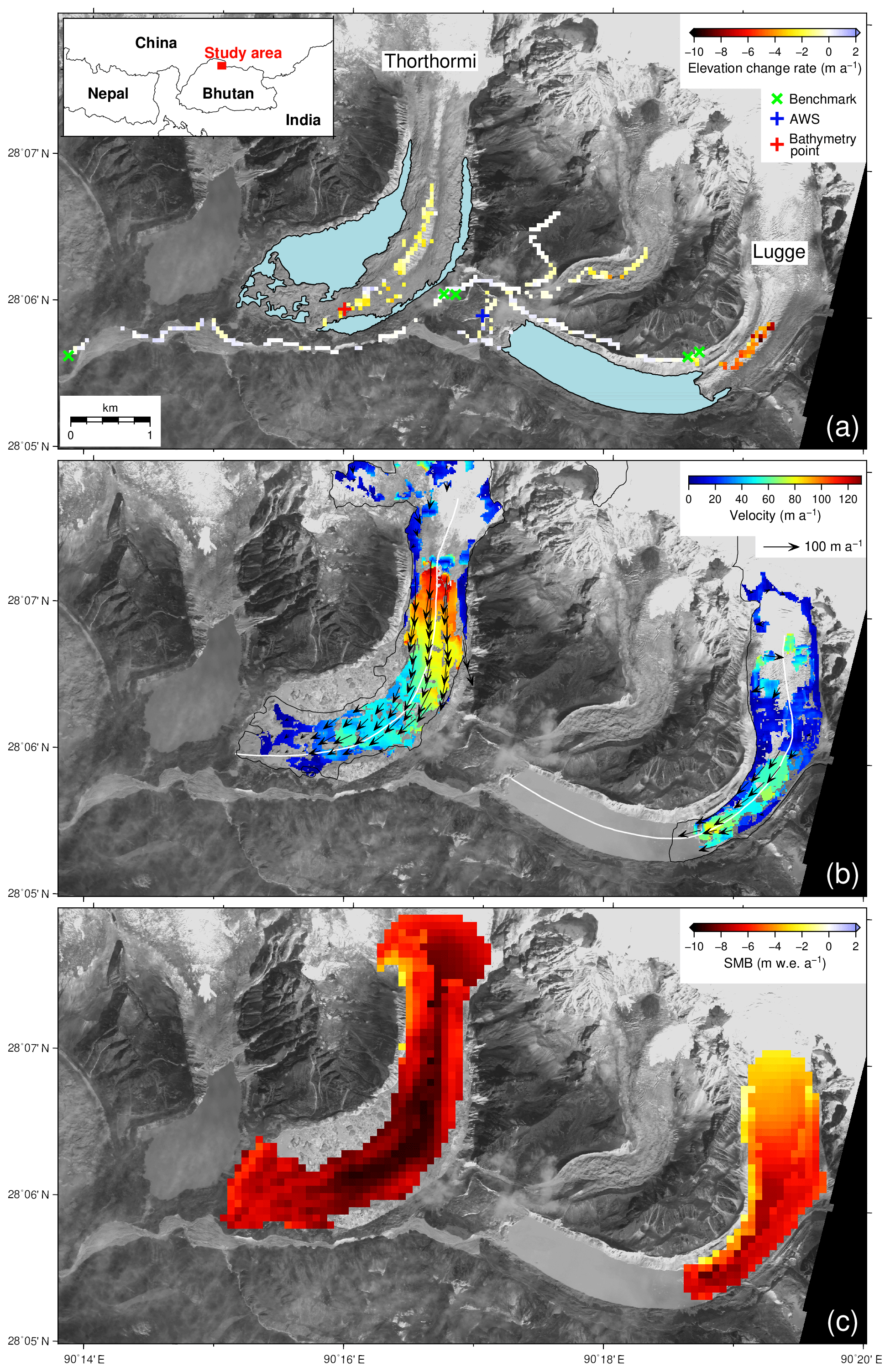
Figure 1 Glaciers and glacial lakes in the Lunana region, Bhutanese Himalaya, superimposed with (a) rate of elevation change (Δz_s∕Δt) for the 2004–2011 period derived from DGPS-DEMs, (b) surface flow velocities (arrows) with magnitude (colour scale) between 30 January 2007 and 1 January 2008, and (c) simulated surface mass balance (SMB) for the 1979–2017 period. The inset map in (a) shows the location of the study site. The Δz_s∕Δt in (a) is depicted on a 50 m grid, which is averaged from the differentiated 1 m DEMs. Note that the bathymetry of Thorthormi Lake was measured at a limited point due to icebergs (red cross). Light blue hatches indicate glacial lakes in December 2009 (Ukita et al., 2011; Nagai et al., 2017). The background image is of the ALOS PRISM scene on 2 December 2009. The white lines in (b) indicate the central flow line of each glacier.

Lugge Glacier is a lake-terminating glacier with an area of 10.93 km² in May 2010 (Table S1, Nagai et al., 2016). The mean surface slope is 12^∘ within 3000 m of the terminus. A moraine-dammed proglacial lake has expanded since the 1960s (Ageta et al., 2000; Komori, 2008), and the glacier terminus retreated by ∼1 km during 1990–2010 (Bajracharya et al., 2014). Lugge Glacier thinned near the terminus at a rate of −8 m a⁻¹ during 2000–2010 (Gardelle et al., 2013). On 7 October 1994, an outburst flood, with a volume of 17.2×10⁶ m³, occurred from Lugge glacial lake (Fujita et al., 2008). The depth of Lugge glacial lake was 126 m at its deepest location, with a mean depth of 50 m, based on a bathymetric survey in September 2002 (Yamada et al., 2004).

Although the debris thickness was not measured during the field campaigns, there were regions of debris-free ice across the ablation areas of Thorthormi and Lugge glaciers (Fig. S1). Debris cover is therefore considered to be thin across the study area. Furthermore, few supraglacial ponds and ice cliffs were observed across the glaciers. Satellite imagery shows that the surface is heavily crevassed in the lower ablation areas, suggesting that surface meltwater drains immediately into the glaciers.

Meteorological and glaciological in situ observations were acquired across the glaciers and lakes in the Lunana region from 2002 to 2004 (Yamada et al., 2004). Naito et al. (2012) reported changes in surface elevation and ice flow velocity along the central flow line in the lower parts of Thorthormi and Lugge glaciers for the 2002–2004 period. The ice thickness change at Lugge Glacier was approximately −5 m a⁻¹ during 2002–2004, which is much more negative than that at Thorthormi Glacier (less than −3 m a⁻¹). The surface flow velocities of Thorthormi Glacier decrease down-glacier from ∼90 to ∼30 m a⁻¹ at 2000–3000 m from the terminus, while the surface flow velocities of Lugge Glacier are nearly uniform at 40–55 m a⁻¹ within 1500 m of the terminus (Naito et al., 2012).

3 Data and methods

3.1 Surface elevation change

We surveyed the surface elevations in the lower parts of Thorthormi and Lugge glaciers from 19 to 22 September 2011 and then compared them with those observed from 29 September to 10 October 2004 (Fujita et al., 2008). We used dual- and single-frequency carrier-phase GPS receivers (GNSS Technologies, GEM-1, and MAGELLAN ProMark3). One receiver was installed 2.5 km west of the terminus of Thorthormi Glacier as a reference station (Fig. 1a), whose location was determined by an online precise point positioning processing service (https://webapp.geod.nrcan.gc.ca/geod/tools-outils/ppp.php?locale=en, last access: 10 July 2019), which provided standard deviations of <4 mm for both the horizontal and vertical coordinates after 1 week of continuous measurements in 2011. Observers walked on and around the glaciers with a GPS receiver and antenna fixed to a frame pack. The height uncertainty of the GPS antenna during the survey was <0.1 m (Tsutaki et al., 2016). The DGPS data were processed with RTKLIB, an open-source software for GNSS positioning (http://www.rtklib.com/, last access: 10 July 2019). Coordinates were projected onto a common Universal Transverse Mercator projection (UTM zone 46N, WGS84 reference system). We generated 1 m DEMs by interpolating the surveyed points with an inverse distance-weighted method, as used in previous studies (e.g. Fujita and Nuimura, 2011; Tshering and Fujita, 2016). The 2004 survey data were calibrated using four benchmarks around the glaciers (Fig. 1a) to generate a 1 m DEM. Details of the 2004 and 2011 DGPS surveys, along with their respective DEMs, are summarised in Table S1. The surface elevation changes between 2004 and 2011 were computed at points where data were available for both dates. Elevation changes were obtained at 431 and 248 DEM grid points for Thorthormi and Lugge glaciers, respectively (Table 1).

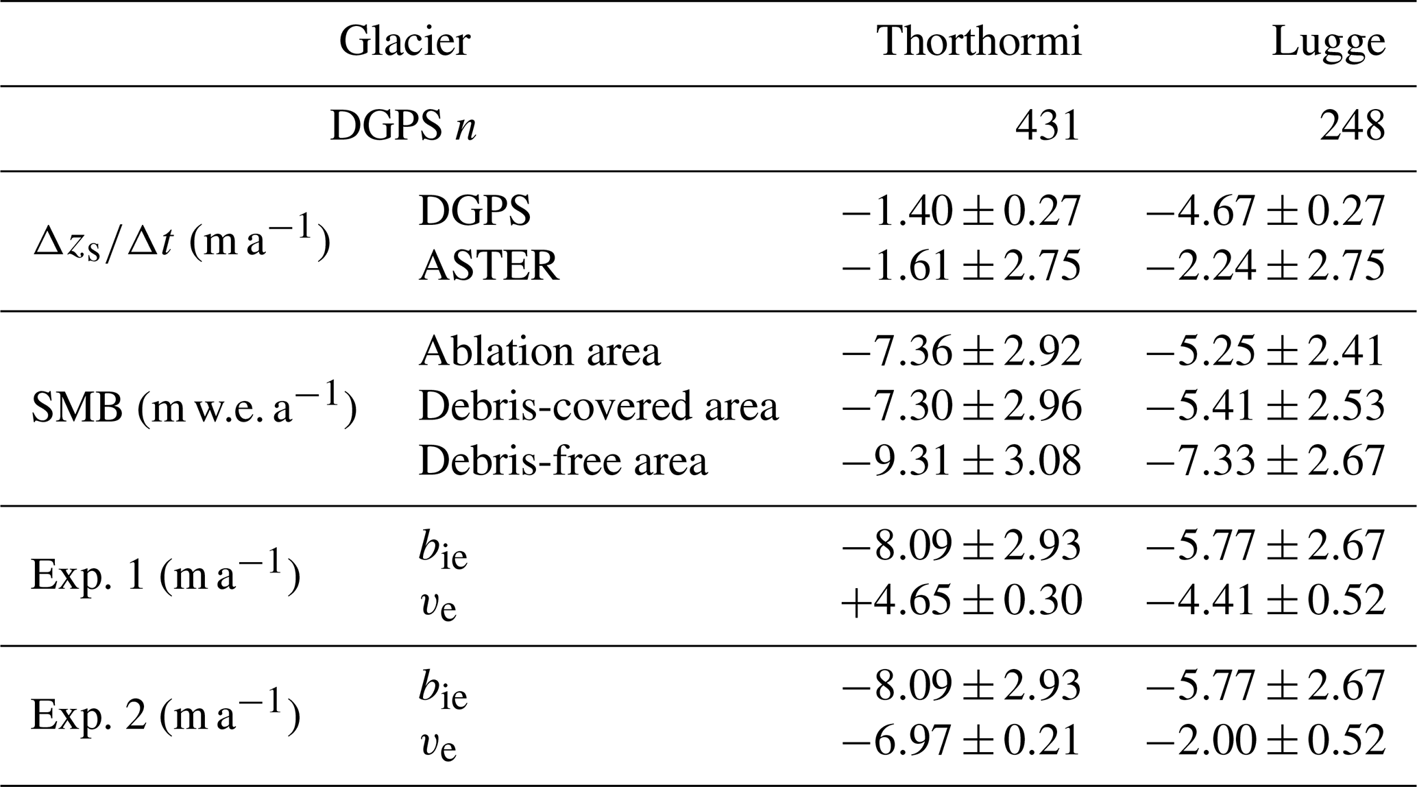
Table 1 Observed rate of elevation changes (Δz_s∕Δt), calculated surface mass balance (SMB), and simulated emergence velocity (v_e) for the ablation area of Thorthormi and Lugge glaciers in the Lunana region, Bhutanese Himalaya. b_ie denotes ice-equivalent SMB.

To evaluate the spatial representativeness of the change in glacier surface elevation derived from the DGPS measurements, we compared the elevation changes derived from the DGPS-DEMs and Advanced Spaceborne Thermal Emission and Reflection Radiometer (ASTER) DEMs acquired on 11 October 2004 and 6 April 2011 (Table S2), respectively, which cover a similar period to our field campaigns (2004–2011). The 30 m ASTER-DEMs were provided by the ASTER-VA (https://gbank.gsj.jp/madas/map/index.html, last access: 10 July 2019). The ASTER-DEM elevations were calibrated using the DGPS data from the off-glacier terrain in 2011. The vertical coordinates of the ASTER-DEMs were then corrected for the corresponding bias, with the elevation change over the glacier surface computed as the difference between the calibrated DEMs.

The horizontal uncertainty of the DGPS survey was evaluated by comparing the positions of the four benchmarks installed around Thorthormi and Lugge glaciers (Fig. 1a). Although previous studies utilising satellite-based DEMs have adopted the standard error as the vertical uncertainty, which assumed uncorrelated noise (e.g. Berthier et al., 2007; Bolch et al., 2011; Maurer et al., 2016), we used the standard deviation of the elevation difference on the off-glacier terrain in the DGPS surveys, which assumed systematic errors because the large number of off-glacier points in our DGPS-DEM survey (n=3893) yielded an extremely small standard error. The actual horizontal uncertainty is likely the function of a noise correlated on a certain spatial scale (e.g. Rolstad et al., 2009; Motyka et al., 2010).

3.2 Surface flow velocities

We calculated surface flow velocities by processing ASTER images (15 m resolution, near infrared, near nadir 3N band) with the COSI-Corr feature tracking software (Leprince et al., 2007), which is commonly adopted in mountainous terrains to measure surface displacements with an accuracy of 1∕4 to 1∕10 of the pixel size (e.g. Heid and Kääb, 2012; Scherler and Strecker, 2012; Lamsal et al., 2017). Orthorectification and coregistration of the images were performed by Japan Space Systems before processing. The orthorectification and coregistration accuracies were reported as 16.9 m and 0.05 pixels, respectively. We selected five image pairs from seven scenes between 22 October 2002 and 12 October 2010, with temporal separations ranging from 273 to 712 d (Table S3), to obtain the annual surface flow velocities of the glaciers. It should be noted that the aim of our flow velocity measurements is to investigate the mean surface flow regimes of the glaciers rather than their interannual variabilities. The subpixel displacement of features on the glacier surface was recorded at every fourth pixel in the orthorectified ASTER images, providing the horizontal flow velocities at 60 m resolution (Scherler et al., 2011). We used a statistical correlation mode, with a correlation window size of 16×16 pixels and a mask threshold of 0.9 for noise reduction (Leprince et al., 2007). The obtained ice flow velocity fields were filtered to remove residual attitude effects and miscorrelations (Scherler et al., 2011; Scherler and Strecker, 2012). We applied two filters to eliminate those flow vectors with large magnitude (greater than ±1σ) and/or direction (>20^∘) deviations from the mean vector within the neighbouring 21×21 pixels.

3.3 Glacier lake area

We analysed variations in the glacial lake area of Thorthormi and Lugge glaciers using 12 satellite images acquired by the Landsat 7 ETM+ between November 2000 and December 2011 (distributed by the United States Geological Survey, http://landsat.usgs.gov/, last access: 10 July 2019). We selected images taken in either November or December with the least snow and cloud cover. We also analysed multiple ETM+ images acquired from the October to December timeframe of each year to avoid the scan line corrector-off gaps. Glacial lakes were manually delineated on false colour composite images (bands 3–5, 30 m spatial resolution). Following previous delineation methods (e.g. Bajracharya et al., 2014; Nuimura et al., 2015; Nagai et al., 2016), marginal ponds in contact with bedrock and moraine ridges were included in the glacial lake area, whereas small supraglacial ponds surrounded by ice were excluded. The accuracy of the outline mapping is equivalent to the image resolution (30 m). The coregistration error in the repeated images was ±30 m, based on visual inspection of the horizontal shift of a stable bedrock and lateral moraines on the coregistered imagery. The user-induced error was estimated to be 5 % of the lake area delineated from the Landsat images (Paul et al., 2013). The total errors of the analysed areas were less than ±0.14 and ±0.08 km⁻¹ for Thorthormi and Lugge glaciers, respectively.

3.4 Mass balance of the debris-covered surface

SMB is an essential component of ice thickness change, but no in situ SMB data are available in the Lunana region. Therefore, the spatial distributions of the SMB on the debris-covered Thorthormi and Lugge glaciers were computed with a heat and mass balance model, which quantifies the spatial distribution of the mean SMB for each glacier.

Thin debris accelerates ice melt by lowering surface albedo, while thick debris (generally more than ∼5 cm) suppresses ice melt and acts as an insulating layer (Østrem, 1959; Mattson et al., 1993). To obtain the spatial distributions of debris thickness and SMB, we estimated the thermal resistance from remotely sensed data and reanalysis climate data (Suzuki et al., 2007a; Zhang et al., 2011; Fujita and Sakai, 2014). The thermal resistance (R_T, m² K W⁻¹) is defined as follows:

$$\begin{array}{}\text{(1)}& R_{\mathrm{T}}={\displaystyle \frac{h_{\mathrm{d}}}{\mathit{\lambda }}},\end{array}$$

where h_d and λ are debris thickness (m) and thermal conductivity (W m⁻¹ K⁻¹), respectively. This method has been applied to reproduce debris thickness and SMB in southeastern Tibet (Zhang et al., 2011) and glacier runoff in the Nepalese Himalaya (Fujita and Sakai, 2014). Assuming no changes in heat storage, the linear temperature profiles within the debris layer and the melting point temperature at the ice–debris interface (T_i, 0 ^∘C), the conductive heat flux through the debris layer (G_d, W m⁻²) and the heat balance at the debris surface are described as follows:

$$\begin{array}{}\text{(2)}& G_{\mathrm{d}}={\displaystyle \frac{(T_{\mathrm{s}}-T_{\mathrm{i}})}{R_{\mathrm{T}}}}=(\mathrm{1}-{\mathit{\alpha }}_{\mathrm{d}})R_{\mathrm{Sd}}+R_{\mathrm{Ld}}-R_{\mathrm{Lu}}+H_{\mathrm{S}}+H_{\mathrm{L}},\end{array}$$

where α_d is the debris surface albedo; R_Sd, R_Ld, and R_Lu are the downward shortwave radiation and downward and upward longwave radiation, respectively (positive sign, W m⁻²); and H_S and H_L are the sensible and latent heat fluxes (W m⁻²), respectively, which are positive when the fluxes are directed toward the ground. Both turbulent fluxes were ignored in the original method to obtain the thermal resistance, based on a sensitivity analysis and field measurements (Suzuki et al., 2007a). However, we improved the method by taking the sensible heat into account because several studies have indicated that ignoring the sensible heat can result in an underestimation of the thermal resistance (e.g. Reid and Brock, 2010). Using eight ASTER images (90 m resolution, Level 3A1 data) obtained between October 2002 and October 2010 (Table S4), along with the NCEP/NCAR reanalysis climate data (NCEP-2, Kanamitsu et al., 2002), we calculated the distribution of mean thermal resistance on the two target glaciers. The surface albedo is calculated using three visible near-infrared sensors (bands 1–3), and the surface temperature is obtained from an average of five thermal infrared sensors (bands 10–14). Automatic weather station (AWS) observations from the terminal moraine of Lugge glacial lake (4524 m a.s.l., Fig. 1a) showed that the annual mean air temperature was ∼0 ^∘C during 2002–2004, and the annual precipitation was 900 mm in 2003 (Suzuki et al., 2007b). The air temperature at the AWS elevation was estimated using the pressure level atmospheric temperature and geopotential height (Sakai et al., 2015) and then modified for each 90×90 m mesh grid points using a single temperature lapse rate (0.006 ^∘C km⁻¹). The wind speed was assumed to be 2.0 m s⁻¹, which is the 2-year average of the 2002–2004 AWS record (Suzuki et al., 2007b). The uncertainties in the thermal resistance and albedo were evaluated as 107 % and 40 %, respectively, by taking the standard deviations calculated from multiple images at the same location (Fig. S2).

The SMB of the debris-covered ablation area was calculated by a heat and mass balance model that included debris-covered effects (Fujita and Sakai, 2014). First, the surface temperature is determined to satisfy Eq. (2) using the estimated thermal resistance and an iterative calculation, and then if the heat flux toward the ice–debris interface is positive, the daily amount of ice melt beneath the debris mantle (M_d, kg m⁻² d⁻¹) is obtained as follows:

$$\begin{array}{}\text{(3)}& M_{\mathrm{d}}={\displaystyle \frac{t_{\mathrm{D}}{G}_{\mathrm{d}}}{l_m}},\end{array}$$

where t_D is the length of a day in seconds (86 400 s) and l_m is the latent heat of fusion of ice (3.33×10⁵ J kg⁻¹). The annual mass balance of the debris-covered part (b, m w.e. a⁻¹) is expressed as follows:

$$\begin{array}{}\text{(4)}& \begin{array}{rl}& b=\\ & \sum _{D=\mathrm{1}}^{\mathrm{365}}{\displaystyle \frac{(P_{\mathrm{s}}+P_{\mathrm{r}}+{\frac{t_{\mathrm{D}}{H}_{\mathrm{L}}}{l_m}}_{\text{for debris}}+{\frac{t_{\mathrm{D}}{H}_{\mathrm{L}}}{l_m}}_{\text{for snow}}-D_{\mathrm{d}}-D_{\mathrm{s}})}{{\mathit{\rho }}_{\mathrm{w}}}}\end{array},\end{array}$$

where ρ_w is the water density (1000 kg m⁻³), P_s and P_r represent snow and rain precipitation, respectively, and D_d and D_s are the daily discharge from debris and snow surfaces, respectively. The precipitation phase is temperature dependent, with the probability of solid and liquid precipitation varying linearly between 0 (100 % snow) and 4 ^∘C (100 % rain) (Fujita and Ageta, 2000). Evaporation from the debris and snow surfaces is expressed in the same formula (not shown), but they are calculated in different schemes because the temperature and saturation conditions of the debris and snow surfaces are different. Discharge and evaporation from the snow surface were only calculated when a snow layer covered the debris surface. Since there is no snow layer present at either the end of the melting season in the current climate condition or at the elevation of the debris-covered area, snow accumulation (P_s) is compensated by with evaporation and discharge from the snow surface during a calculation year. D_d is expressed as follows:

$$\begin{array}{}\text{(5)}& D_{\mathrm{d}}=M_{\mathrm{d}}+P_{\mathrm{r}}+{{\displaystyle \frac{t_{\mathrm{D}}{H}_{\mathrm{L}}}{l_m}}}_{\text{for debris}},\end{array}$$

which then simplifies the mass balance to

$$\begin{array}{}\text{(6)}& b=\sum _{D=\mathrm{1}}^{\mathrm{365}}{\displaystyle \frac{M_{\mathrm{d}}}{{\mathit{\rho }}_{\mathrm{w}}}}.\end{array}$$

This implies that the mass balance of the debris-covered area is equivalent to the amount of ice melt beneath the debris mantle. Further details on the equations and methodology used in the model are described by Fujita and Sakai (2014). The mass balance was calculated at 90×90 m mesh grid points on the ablation area of the two glaciers using 38 years of ERA-Interim reanalysis data (1979–2017, Dee et al., 2011), with the results given in metres of water equivalent (w.e.). The meteorological variables in the ERA-Interim reanalysis data (2002–2004) were calibrated with in situ meteorological data (2002–2004) from the terminal moraine of Lugge Glacier (Fig. S3). The ERA-Interim wind speed was simply multiplied by 1.3 to obtain the same average as in the observational data. The SMBs calculated with the observed and calibrated ERA-Interim data for 2002–2004 were compared with those from the entire 38-year ERA-Interim data set. The SMBs for 2002–2004 (from both the observational and ERA-Interim data sets) show no clear anomaly against the long-term mean SMB (1979–2017) (Fig. S4).

The sensitivity of the simulated meltwater was evaluated against the meteorological parameters used in the SMB model. We chose meltwater instead of SMB to quantify the uncertainty because the SMB uncertainty cannot be expressed as a percentage. The tested parameters are surface albedo, air temperature, precipitation, relative humidity, solar radiation, thermal resistance, and wind speed. The thermal resistance and albedo uncertainties were based on the standard deviations derived from the eight ASTER images used to estimate these parameters (Fig. S2). Each meteorological variable's uncertainty, with the exceptions of the thermal resistance and albedo uncertainties, was assumed to be the root-mean-square error (RMSE) of the ERA-Interim reanalysis data against the observational data (Fig. S3). The simulated meltwater uncertainty was estimated as the variation in meltwater within a possible parameter range via a quadratic sum of the results from each meteorological parameter.

3.5 Ice dynamics

3.5.1 Model descriptions

To investigate the dynamically induced ice thickness change, numerical experiments were carried out by applying a two- dimensional ice flow model to the longitudinal cross sections of Thorthormi and Lugge glaciers. The aim of the experiments was to investigate whether the ice thickness changes observed at the glaciers were affected by the presence of proglacial lakes.

The model was developed for a land-terminating glacier (Sugiyama et al., 2003, 2014) and is applied to a lake-terminating glacier in this study. Taking the x and z coordinates in the along-flow and vertical directions, the momentum and mass conservation equations in the x–z plane are:

$$\begin{array}{}\text{(7)}& {\displaystyle }& {\displaystyle \frac{\partial {\mathit{\sigma }}_{xx}}{{\partial }_x}}+{\displaystyle \frac{\partial {\mathit{\sigma }}_{xz}}{{\partial }_z}}=\mathrm{0},\text{(8)}& {\displaystyle }& {\displaystyle \frac{\partial {\mathit{\sigma }}_{zx}}{{\partial }_x}}+{\displaystyle \frac{\partial {\mathit{\sigma }}_{zz}}{{\partial }_z}}={\mathit{\rho }}_i\mathit{g},\end{array}$$

and

$$\begin{array}{}\text{(9)}& {\displaystyle \frac{\partial {\mathit{u}}_x}{{\partial }_x}}+{\displaystyle \frac{\partial {\mathit{u}}_z}{{\partial }_z}}=\mathrm{0},\end{array}$$

where σ_ij (i, j = x, z) is the components of the Cauchy stress tensor, ρ_i is the density of ice (910 kg m⁻³), g is the gravitational acceleration vector (9.81 m s⁻²), and u_x and u_z are the horizontal and vertical components of the flow velocity vector, respectively. The stress in Eqs. (8) and (9) is linked to the strain rate via the constitutive equation given by Glen’s flow law (Glen, 1955):

$$\begin{array}{}\text{(10)}& {\dot{\mathit{ϵ}}}_{ij}=A{\mathit{\tau }}_{\mathrm{e}}^{n-\mathrm{1}}{\mathit{\tau }}_{ij},\end{array}$$

where ${\dot{\mathit{ϵ}}}_{ij}$ and τ_ij are the components of the strain rate and deviatoric stress tensors, respectively, and τ_e is the effective stress, which is defined as

$$\begin{array}{}\text{(11)}& {\mathit{\tau }}_{\mathrm{e}}={\displaystyle \frac{\mathrm{1}}{\mathrm{2}}}({\mathit{\tau }}_{xx}^{\mathrm{2}}+{\mathit{\tau }}_{zz}^{\mathrm{2}})+{\mathit{\tau }}_{xz}^{\mathrm{2}}.\end{array}$$

The rate factor (A, MPa⁻³ a⁻¹) and flow law exponent (n) are material parameters. We used the commonly accepted value of n=3 for the flow law exponent and employed a rate factor of A=75 MPa⁻³ a⁻¹, which was previously used to model a temperate valley glacier (Gudmundsson, 1999). We assumed the glaciers were temperate. This assumption was based on a measured mean annual air temperature of ∼0 ^∘C on the terminal moraine of Lugge Glacier (Suzuki et al., 2007b).

The model domain extended from 5100 and 3500 m to the termini of Thorthormi and Lugge glaciers, respectively (white lines in Fig. 1b), and included the ablation and lower accumulation areas of both glaciers. We only interpret the results from the ablation areas (0–4300 and 500–1900 m from the termini of Thorthormi and Lugge glaciers, respectively), with the surface flow velocities obtained from the ASTER imagery. The lower accumulation area was included in the model domain to supply ice to the study region, but it was excluded from analysis of the results. The surface elevation of the model domain ranges from 4443 to 4846 m for Thorthormi Glacier, and from 4511 to 5351 m for Lugge Glacier. The surface geometry was obtained from the 90 m ASTER GDEM version 2, obtained in November 2001 after smoothing the elevations at a bandwidth of 200 m. The ice thickness distribution was estimated from a method proposed for alpine glaciers (Farinotti et al., 2009) with the same rate factor (A=75 MPa⁻³ a⁻¹), the above-mentioned SMB model (Sect. 3.4), and satellite-based ice thickness change (Sect. 3.1). We applied the same local regression filter to smooth the estimated bedrock geometry. The bedrock elevation of Thorthormi Glacier was constrained by bathymetry data acquired in September 2011 at 1400 m from the terminus (red cross in Fig. 1a). For Lugge Glacier, the bed elevation at the glacier front was estimated from the bathymetric map of Lugge glacial lake, surveyed in September 2002 (Yamada et al., 2004). Using the observed ice thickness data as constraints, we determined the correction factors for the method of Farinotti et al. (2009) to be 0.78 and 0.36 for Thorthormi and Lugge glaciers, respectively. These factors include the effects of basal sliding, the geometry of the glacier cross section, and other processes (Eq. 7 in Farinotti et al., 2009). To solve Eqs. (8) and (9) for u_x and u_z, the modelled domain was discretised with a finite element mesh. The mesh resolution was 100 m in the horizontal direction, several metres near the bed and 4–67 m near the surface in the vertical direction. The total number of elements was 612 and 420 for Thorthormi and Lugge glaciers, respectively. Additional experiments with a finer mesh resolution confirmed convergence of ice flow velocity within 4 %.

The glacier surface was assumed to be stress-free, and the ice flux through the up-glacier model boundary was prescribed from the surface velocity field obtained via the satellite analysis. We applied a fourth-order function for the velocity profile from the surface to the bed. The basal sliding velocity (u_b) was given as a linear function of the basal shear traction (τ_xz,b):

$$\begin{array}{}\text{(12)}& {\mathit{u}}_{\mathrm{b}}=C\left(x\right){\mathit{\tau }}_{xz,\mathrm{b}},\end{array}$$

where C is the sliding coefficient. We used spatially variable sliding coefficients, which were obtained by minimising the RMSE between the modelled and measured surface flow velocities within 0–4300 and 500–1900 m of the termini of Thorthormi and Lugge glaciers, respectively (Fig. S5).

3.5.2 Experimental configurations

To quantify the effect of glacier dynamics on ice thickness change, we performed two experiments for Thorthormi and Lugge glaciers. Experiment 1 was performed to compute the ice flow velocity fields under the present terminus conditions. In this experiment, Thorthormi Glacier was treated as a land-terminating glacier with no horizontal ice motion at the glacier front, whereas Lugge Glacier was treated as a lake-terminating glacier by applying hydrostatic pressure at the front as a function of water depth. A stress-free boundary condition was given to the calving front above the lake level. We used the 2001 glacier surface elevation and 2004 supraglacial pond and proglacial lake water levels as boundary conditions (Fujita et al., 2008).

Experiment 2 was designed to investigate the influence of proglacial lakes on glacier dynamics. For Thorthormi Glacier, we simulated a calving front with thickness of 125 m. The position of the hypothetical calving front was set where the lake depth was acquired during a bathymetry survey in September 2011 (red cross in Fig. 1a). The surface level of the proglacial lake was assumed to be 4432 m a.s.l., which is the mean surface level of the supraglacial ponds measured in September 2004 (Fujita et al., 2008). Hydrostatic pressure and stress-free conditions were applied to the lower boundary below and above the lake level, respectively. For Lugge Glacier, we simulated a lake-free situation, with ice flowing to the contemporary terminal moraine, so that the glacier terminates on land. Bedrock topography is derived from the bathymetric map (white lines in Fig. 1b, Yamada et al., 2004). The surface topography is linearly extrapolated from the surface elevations at the calving front in 2002, with the ice thickness reduced to a negligibly small value at the glacier front. In the experiment, we used 444 and 684 elements for Thorthormi and Lugge glaciers, respectively.

3.5.3 Emergence velocity

To compare the influence of ice dynamics on glacier thickness change in lake- and land-terminating glaciers, we calculated the emergence velocity (v_e) as follows:

$$\begin{array}{}\text{(13)}& v_{\mathrm{e}}=v_z-v_h\tan \mathit{\alpha },\end{array}$$

where v_z and v_h are the vertical and horizontal flow velocities, respectively, and α is the surface slope (Cuffey and Paterson, 2010). The surface slope α was obtained every 100 m from the surface topography of the ice flow model.

4 Results

4.1 Surface elevation change

Figure 1a shows the rates of surface elevation change (Δz_s∕Δt) for Thorthormi and Lugge glaciers from 2004 to 2011 derived from the DGPS-DEMs. The rates for Thorthormi Glacier range from −3.37 to +1.14 m a⁻¹, with a mean rate of −1.40 m a⁻¹ (Table 1). These rates show large variability within the limited elevation band (4410–4450 m a.s.l., Fig. 2b). No clear trend is observed at 1000–3000 m from the terminus (Fig. 2c). The rates for Lugge Glacier range from −9.13 to −1.30 m a⁻¹, with a mean rate of −4.67 m a⁻¹ (Table 1). The most negative values (−9 m a⁻¹) are found at the lower glacier elevations (4560 m a.s.l., Fig. 2b), which correspond to 1300 m from the 2002 terminus position (Fig. 2c). The RMSE between the surveyed positions (five measurements in total, with one or two measurements for each benchmark) is 0.21 m in the horizontal direction. The mean elevation difference between the 2004 and 2011 DGPS-DEMs is 0.48 m, with a standard deviation of 1.91 m (Fig. 2a), which yield an uncertainty in the elevation change rate of 0.27 m a⁻¹. The uncertainties in the elevation change rate of the ASTER-DEMs are estimated to be 2.75 m a⁻¹ for the 2004 and 2011 DEMs (Fig. S7). Given the ASTER-DEM uncertainties, the DGPS-DEMs and ASTER-DEMs yield a similar Δz_s∕Δt that falls within the uncertainty ranges in the scatter plots (Figs. S8 and S9), thus supporting the applicability of the DGPS measurements to the entire ablation area.

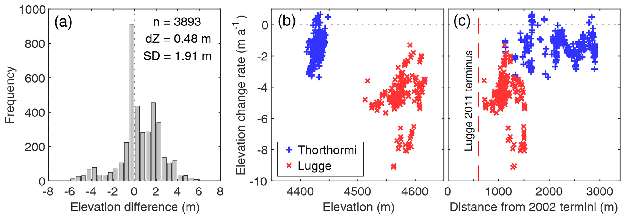
Figure 2 (a) Histogram of elevation differences over off-glacier area at 0.5 m elevation bins. The rate of elevation change for Thorthormi (blue) and Lugge (red) glaciers is compared with (b) elevation in 2011, and (c) distance from the glacier termini in 2002 along the central flow lines (Fig. 1b). The dashed red line in (c) denotes the location of the calving front of Lugge Glacier in 2011.

4.2 Surface flow velocities

Figure 1b shows the surface flow velocity field from 30 January 2007 to 1 January 2008 (337 d). On Thorthormi Glacier, the flow velocities decrease down-glacier, ranging from ∼110 m a⁻¹ at the foot of the icefall to <10 m a⁻¹ at the terminus (Fig. 3a). The flow velocities of Lugge Glacier increase down-glacier, ranging from 20–60 to 50–80 m a⁻¹ within 2000 m of the calving front (Fig. 3b). The flow velocity uncertainty was estimated to be ±12.1 m a⁻¹, as given by the mean off-glacier displacement from 3 February 2006 to 30 January 2007 (362 d) (Fig. S10). If these flow speeds were solely attributed to ice deformation with a frozen bed assumption, ice thickness of the glaciers would be 300 to 800 m, much greater than the bathymetry records (∼100 m), supporting the temperate glacier assumption.

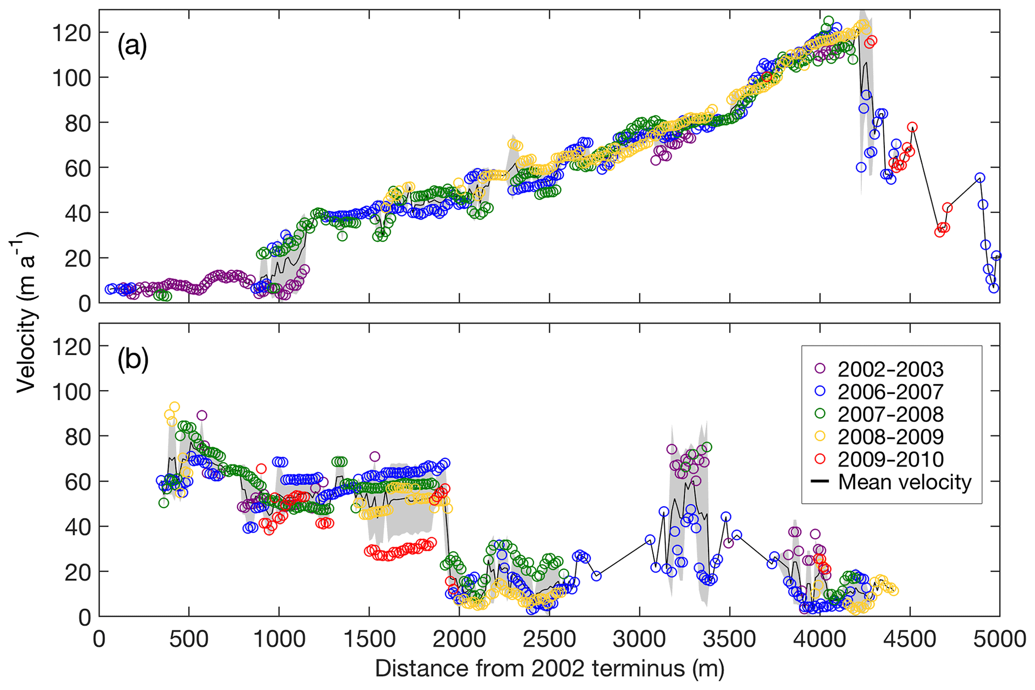
Figure 3 Surface flow velocities along the central flow lines of (a) Thorthormi and (b) Lugge glaciers for the 2002–2010 study period. The black lines are the mean flow velocities from 2002 to 2010, with the shaded grey regions denoting the standard deviation. The distance from each respective 2002 glacier terminus is indicated on the horizontal axis.

4.3 Changes in glacial lake area

The supraglacial pond area near the front of Thorthormi Glacier progressively increased from 2000 to 2011, at a mean rate of 0.09 km² a⁻¹, and Lugge glacial lake also expanded from 2000 to 2011, at a mean rate of 0.03 km² a⁻¹ (Fig. 4). The total area changes from 2000 to 2011 were 1.79 and 0.46 km² for Thorthormi and Lugge glaciers, respectively.

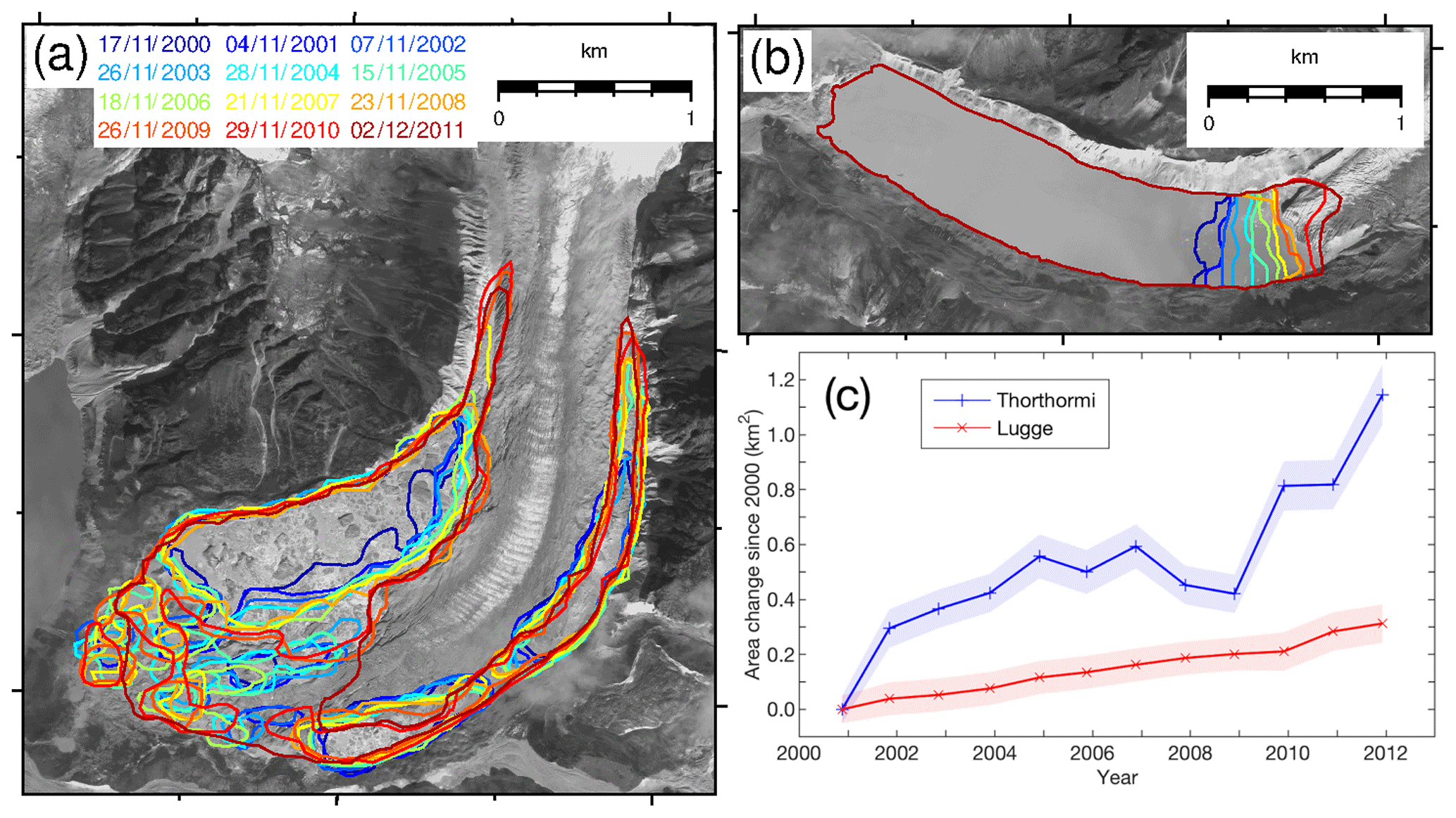
Figure 4 Glacial lake boundaries in (a) Thorthormi and (b) Lugge glaciers from 2000 to 2011 and (c) cumulative lake area changes of the glaciers since 17 November 2000. The background image is an ALOS PRISM image acquired on 2 December 2009.

4.4 Surface mass balance

The simulated mean SMBs over the ablation area were $-\mathrm{7.36}\pm \mathrm{2.92}$ m w.e. a⁻¹ for Thorthormi Glacier and $-\mathrm{5.25}\pm \mathrm{2.41}$ m w.e. a⁻¹ for Lugge Glacier (Fig. 1c, Table 1). The SMB distribution correlates well with the thermal resistance distribution (Fig. S11), with the larger thermal resistance areas suggesting a thicker debris, which results in a reduced SMB. The debris-free surface has a more negative SMB than the debris-covered regions of the glaciers. The mean SMBs of the debris-free and debris-covered surfaces in the ablation area of Thorthormi Glacier are $-\mathrm{9.31}\pm \mathrm{3.08}$ and $-\mathrm{7.30}\pm \mathrm{2.96}$ m w.e. a⁻¹, respectively, while those of Lugge Glacier are $-\mathrm{7.33}\pm \mathrm{2.67}$ and $-\mathrm{5.41}\pm \mathrm{2.53}$ m w.e. a⁻¹, respectively (Table 1). The sensitivity of simulated meltwater in the SMB model was evaluated as a function of the RMSE of each meteorological variable across the debris-covered area (Figs. S12 and S13). Ice melting is more sensitive to solar radiation and thermal resistance. The influence of thermal resistance on meltwater formation is considered to be small since the debris cover is thin over the glaciers. The meltwater uncertainty is estimated to be ∼50 % across most of Thorthormi and Lugge glaciers.

4.5 Numerical experiments of ice dynamics

The ice thinning of Lugge Glacier was 3 times faster than that of Thorthormi Glacier. However, the mean SMB was 1.4 times more negative at Thorthormi Glacier, suggesting a substantial influence of glacier dynamics on ice thickness change. To quantify the contribution of ice dynamics to the ice thickness change, we performed numerical experiments with the present (Experiment 1) and reversed (Experiment 2) glacier geometries.

4.5.1 Experiment 1 – present terminus conditions

Modelled results for the present geometry show significantly different flow velocity fields for Thorthormi and Lugge glaciers (Fig. 5c and d). Thorthormi Glacier flows faster (>100 m a⁻¹) in the upper reaches where the surface is steeper than the other regions (Fig. 5c). Down-glacier of the icefall, where the glacier surface is flatter, the ice motion slows in the down-glacier direction, with the flow velocities decreasing to <10 m a⁻¹ near the terminus (Fig. 5e). Ice flows upward relative to the surface across most of the modelled region (Fig. 5c). In contrast to the down-glacier decrease in the flow velocities at Thorthormi Glacier, the computed velocities of Lugge Glacier are <60 m a⁻¹ within 1000–1900 m of the terminus, and then increase to 90 m a⁻¹ at the calving front (Fig. 5f). Ice flow is nearly parallel or slightly downward relative to the glacier surface (Fig. 5d). The modelled surface flow velocities are in good agreement with the satellite-derived flow velocities within 0–4300 m of the terminus of Thorthormi Glacier (Fig. 5e). The calculated surface flow velocities of Lugge Glacier agree with the satellite-derived flow velocities to ±12 % within 500–1900 m (Fig. 5f).

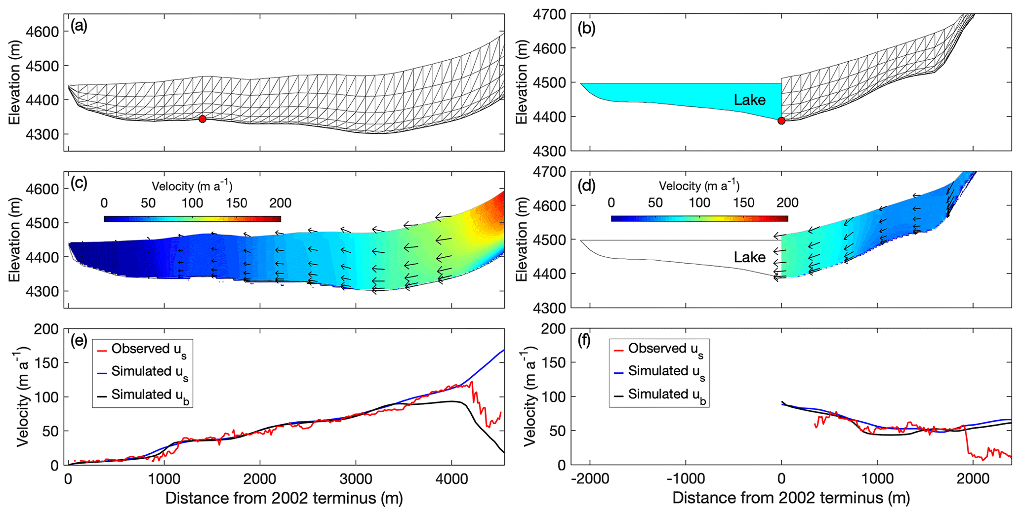
Figure 5 Ice flow simulations in longitudinal cross sections of Thorthormi (a, c, e) and Lugge (b, d, f) glaciers, with the present geometries of the glaciers employed in the models. (a, b) Finite element meshes used for the simulations, with red markers indicating the bedrock elevation based on a bathymetric survey. The light blue shading in (b) indicates Lugge glacial lake. Simulated (c, d) two-dimensional flow vectors (magnitude and direction) and (e, f) horizontal components of the flow velocity. The blue and black curves are the simulated surface (u_s) and basal velocities (u_b), respectively. The red curves are the observed surface flow velocities for 2002–2010.

4.5.2 Experiment 2 – reversed terminus conditions

Figure 6c shows the flow velocities simulated for the lake-terminating boundary condition of Thorthormi Glacier, in which the flow velocities within 200 m of the calving front are 8 times faster than those of Experiment 1 (Figs. 5c and 6c). The mean vertical surface flow velocity within 2000 m of the front is still negative (−11.0 m a⁻¹). The modelled result demonstrates significant acceleration as the glacier dynamics change from a compressive to tensile flow regime after proglacial lake formation. For Lugge Glacier, the flow velocities decrease over the entire glacier in comparison with Experiment 1 (Figs. 5d and 6d). The upward ice motion appears within 2500 m of the terminus. The numerical experiments demonstrate that the formation of a proglacial lake causes significant changes in ice dynamics.

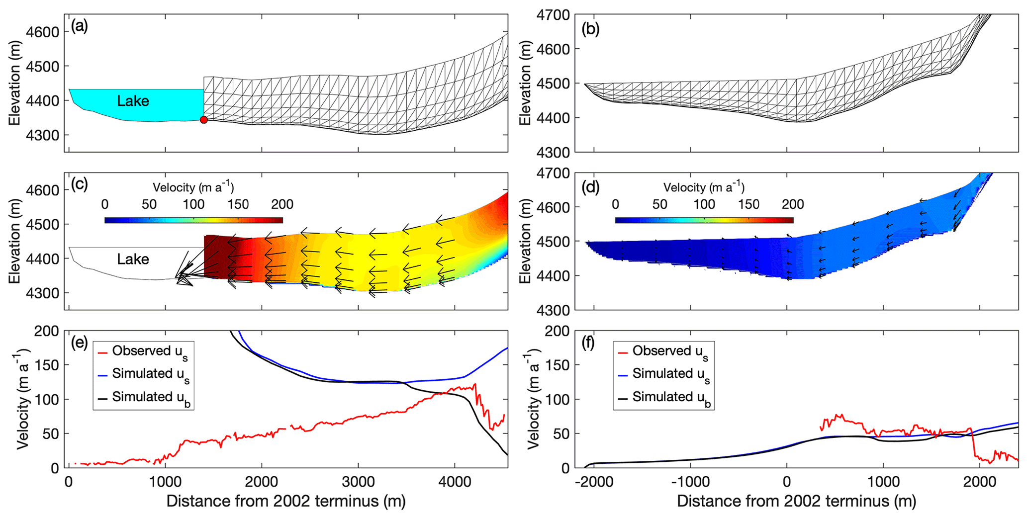
Figure 6 Ice flow simulations in longitudinal cross sections of Thorthormi Glacier under the lake-terminating condition (a, c, e), and Lugge Glacier under the land-terminating condition (b, d, f). (a, b) Finite element meshes used for the simulation. The light blue shading in (a) indicates the proglacial lake in front of Thorthormi Glacier. Simulated (c, d) two-dimensional flow vectors (magnitude and direction) and (e, f) horizontal components of the flow velocity. The blue and black curves are the simulated surface (u_s) and basal velocities (u_b), respectively. The red curves are the observed surface flow velocities for 2002–2010.

4.5.3 Simulated surface flow velocity uncertainty

Basal sliding accounts for 90 % and 91 % of the simulated surface flow velocities in the ablation areas of Thorthormi and Lugge glaciers, respectively (Fig. 5e and f), suggesting that ice deformation plays a minor role in ice dynamics. The standard deviations of the ASTER-derived surface flow velocities are 2.9 and 6.7 m a⁻¹ for Thorthormi and Lugge glaciers, respectively, which are considered to be the interannual variabilities in the measured surface flow velocities (Fig. 3). We performed sensitivity tests of the modelled surface flow velocities by changing the ice thickness and sliding coefficient by ±30 %. The results show that the simulated surface flow velocity of Thorthormi Glacier varies by 33 % and 51 % when the sliding coefficient (C) and ice thickness are varied by ±30 %, respectively (Fig. S14). For Lugge Glacier, the simulated flow velocity varies by 41 % and 39 % when the sliding coefficient and ice thickness are varied by ±30 %, respectively. The mean uncertainty of the simulated surface flow velocity is 7.0 and 6.9 m a⁻¹ for Thorthormi and Lugge glaciers, respectively. Measured surface velocities show step changes at 800–1200 m and 1900–2000 m from the termini of Thorthormi and Lugge glaciers, respectively (Fig. 3). It is likely that these step changes are due to miscorrelation in the feature-tracking process caused by surface ogives along the centre of the glaciers. Consequently, we only interpret the simulated velocities within 500–1900 m of the terminus of Lugge Glacier. For Thorthormi Glacier, we considered a mean value of observed velocities at the area as a reference value of the simulation.

4.6 Emergence velocity

Figure 7 shows the computed emergence velocity and SMB along the central flow lines of the glaciers. Given the computed surface flow velocities from Experiment 1, the emergence velocity of Thorthormi Glacier was 4.65±0.30 m a⁻¹ within 4300 m of the terminus (Fig. 7a). Conversely, the emergence velocity of Lugge Glacier was $-\mathrm{4.41}\pm \mathrm{0.52}$ m a⁻¹ within 500–1900 m of the terminus (Fig. 7a).

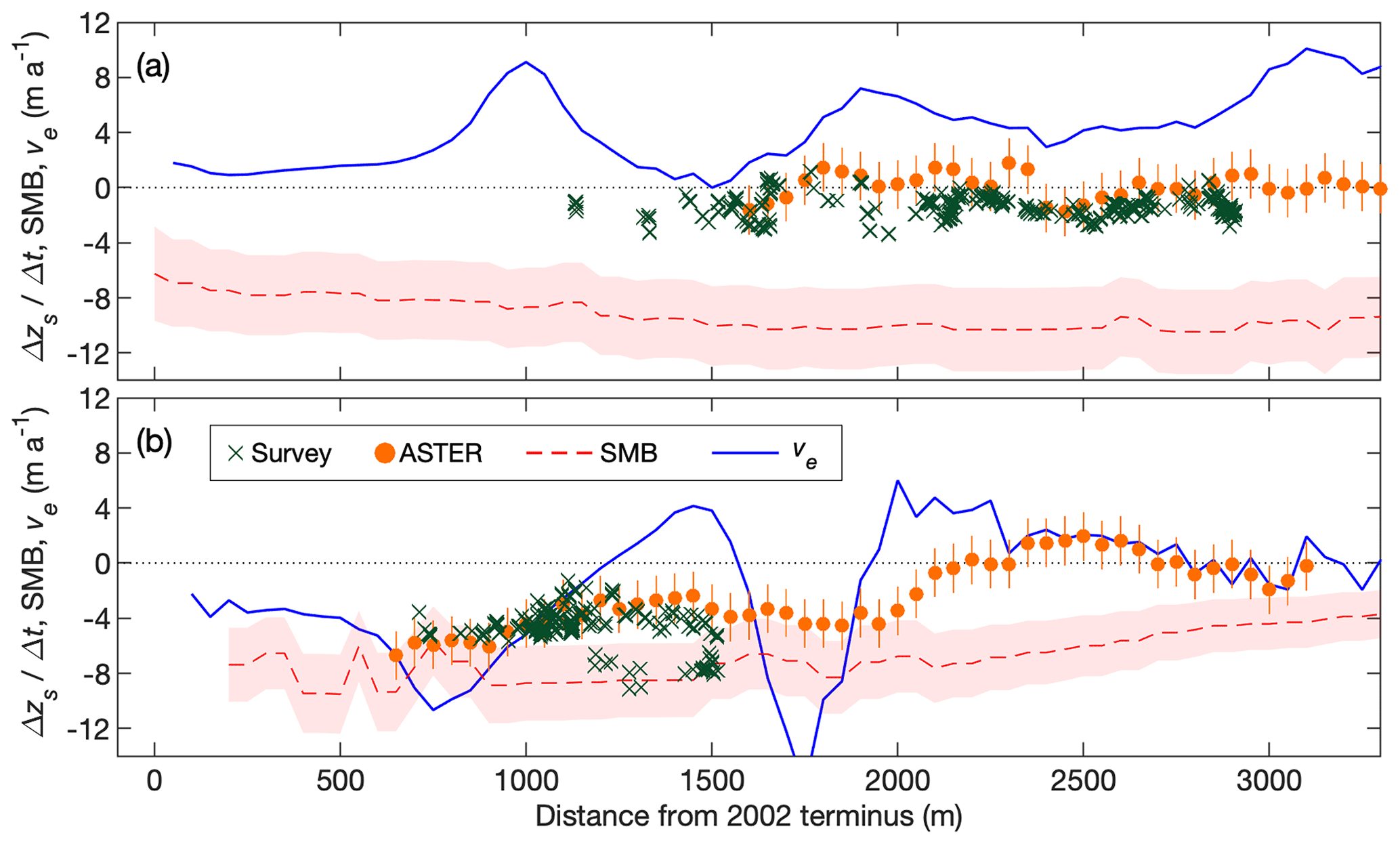
Figure 7 Rate of elevation change (Δz_s∕Δt) from survey and ASTER-DEMs during 2004–2011, simulated surface mass balance (SMB), emergence velocity (v_e) calculations along the central flow lines of (a) Thorthormi and (b) Lugge glaciers. Shaded regions denote the simulated SMB uncertainties.

The emergence velocity computed under reversed terminus conditions (Experiment 2) varies from that computed under the present geometries (Experiment 1) for both Thorthormi and Lugge glaciers (Fig. 8). For the lake-terminating condition of Thorthormi Glacier, the mean emergence velocity becomes negative ($-\mathrm{6.97}\pm \mathrm{0.21}$ m a⁻¹) within 2900 m of the terminus. The mean emergence velocity of Lugge Glacier computed under the land-terminating condition is less negative ($-\mathrm{2.00}\pm \mathrm{0.52}$ m a⁻¹) within 500–1900 m of the present terminus.

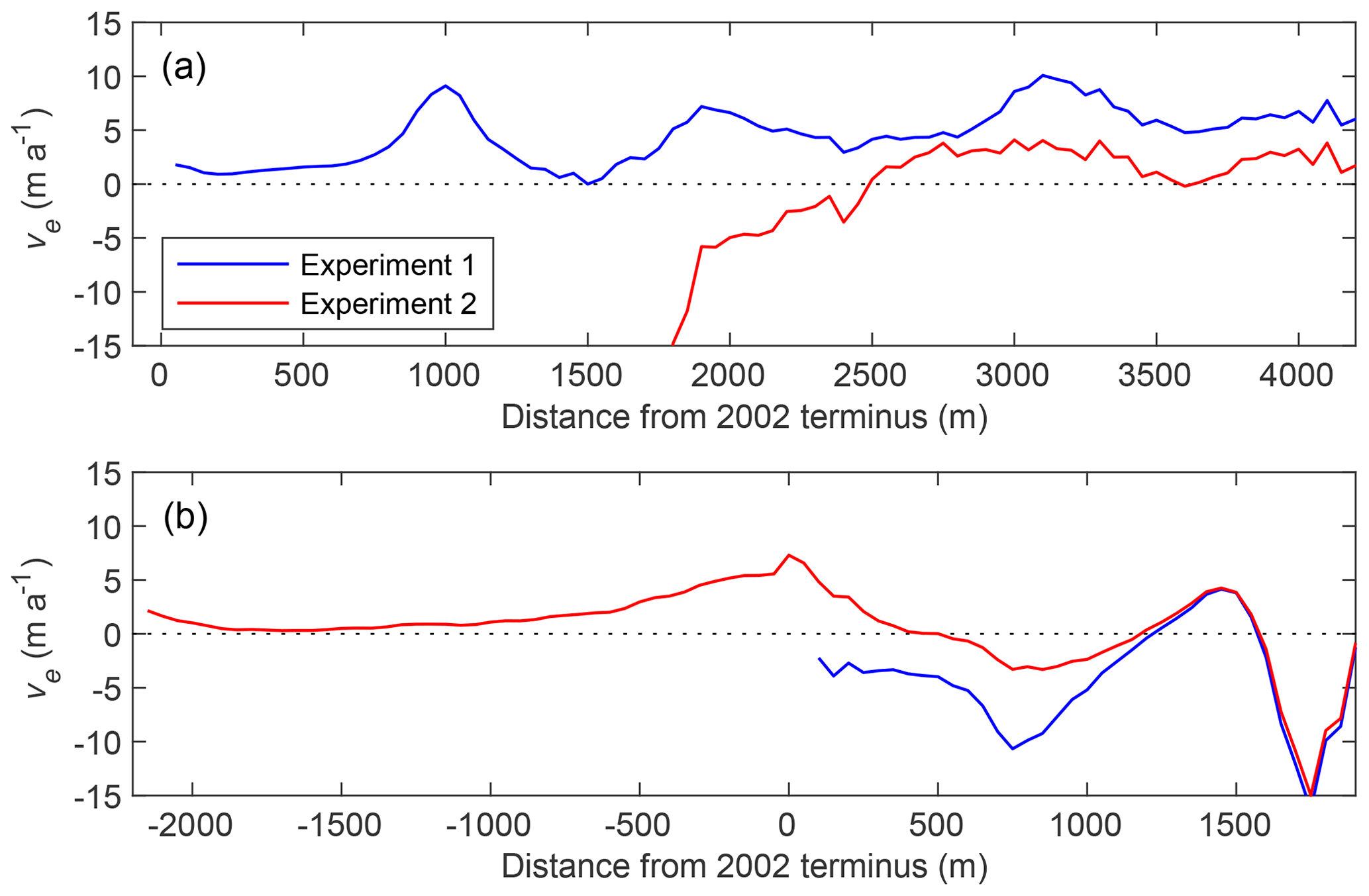
Figure 8 Calculated emergence velocity (v_e) for Experiment 1 and Experiment 2 along the central flow lines of (a) Thorthormi and (b) Lugge glaciers.

5 Discussion

5.1 Glacier thinning

The repeat DGPS surveys revealed rapid thinning of the ablation area of Lugge Glacier between 2004 and 2011. The mean Δz_s∕Δt ($-\mathrm{4.67}\pm \mathrm{0.27}$ m a⁻¹) is comparable to that for the 2002–2004 period (−5 m a⁻¹, Naito et al., 2012), whereas it is more than twice as negative as that derived from the ASTER-DEMs for the 2004–2011 period ($-\mathrm{2.24}\pm \mathrm{2.75}$ m a⁻¹). The results suggest that Lugge Glacier is thinning more rapidly than neighbouring glaciers in the Nepalese and Bhutanese Himalaya. The mean Δz_s∕Δt was $-\mathrm{0.50}\pm \mathrm{0.14}$ m a⁻¹ in the ablation area of Bhutanese glaciers for the 2000–2010 period (Gardelle et al., 2013) and $-\mathrm{2.30}\pm \mathrm{0.53}$ m a⁻¹ for debris-free glaciers in eastern Nepal and Bhutan during 2003–2009 (Kääb et al., 2012). Maurer et al. (2016) reported that the mean Δz_s∕Δt for Lugge Glacier during 1974–2006 ($-\mathrm{0.6}\pm \mathrm{0.2}$ m a⁻¹) was greater than those for other Bhutanese lake-terminating glaciers (−0.2 to −0.4 m a⁻¹). The mean Δz_s∕Δt values of Thorthormi Glacier derived from the DGPS-DEMs ($-\mathrm{1.40}\pm \mathrm{0.27}$ m a⁻¹) and ASTER-DEMs ($-\mathrm{1.61}\pm \mathrm{2.75}$ m a⁻¹) from 2004 to 2011 are comparable with previous measurements, which range from −3 to 0 m a⁻¹ for the 2002–2004 period (Naito et al., 2012). The mean rate across Thorthormi Glacier was $-\mathrm{0.3}\pm \mathrm{0.2}$ m a⁻¹ during 1974–2006 (Maurer et al., 2016), which is a typical rate in the Bhutanese Himalaya.

Lugge Glacier is thinning more rapidly than Thorthormi Glacier, which is consistent with previous satellite-based studies. For example, the Δz_s∕Δt values of the lake-terminating Imja and Lumding glaciers (−1.14 and −3.41 m a⁻¹, respectively) were ∼4 times greater than those of the land-terminating glaciers (approximately −0.87 m a⁻¹) in the Khumbu region of the Nepalese Himalaya (Nuimura et al., 2012). King et al. (2017) measured the Δz_s∕Δt of the lower parts of nine lake-terminating glaciers in the Everest area (approximately −2.5 m a⁻¹), which was 67 % more negative than that of 18 land-terminating glaciers (approximately −1.5 m a⁻¹). The Δz_s∕Δt of lake-terminating glaciers in Yakutat ice field, Alaska (−4.76 m a⁻¹), was ∼30 % more negative than that of the neighbouring land-terminating glaciers (Trüssel et al., 2013).

5.2 Influence of ice dynamics on glacier thinning

The mean SMB of Thorthormi Glacier is 40 % more negative than that of Lugge Glacier. Since there is only a thin debris mantle across the ablation areas of both glaciers (Fig. S1), the more negative SMB of Thorthormi Glacier could be explained by the glacier being situated at lower elevations (Fig. 2b). The modelled SMBs (Thorthormi < Lugge) and observed Δz_s∕Δt values (Lugge < Thorthormi) suggest that the glacier dynamics of these two glaciers are substantially different. The horizontal flow velocities of Lugge Glacier increase toward the terminus along the central flow line (Fig. 5d), and the computed emergence velocity is negative ($-\mathrm{4.41}\pm \mathrm{0.52}$ m a⁻¹), which means the ice dynamics accelerate glacier thinning. Conversely, the flow velocities of Thorthormi Glacier decrease toward the terminus (Fig. 5c), resulting in thickening under a longitudinally compressive flow regime. The emergence velocity of Thorthormi Glacier is positive (4.65±0.30 m a⁻¹), indicating a vertically extending strain regime. This result implies that dynamically induced ice thickening partly compensated for by the negative SMB.

Experiment 1 demonstrates that the difference in emergence velocity between land- and lake-terminating glaciers leads to contrasting thinning patterns. Furthermore, Experiment 2 demonstrates that the emergence velocity was less negative ($-\mathrm{2.00}\pm \mathrm{0.52}$ m a⁻¹) in the absence of a proglacial lake at the front of Lugge Glacier. For Thorthormi Glacier, the emergence velocity under the lake-terminating condition is negative ($-\mathrm{6.97}\pm \mathrm{0.21}$ m a⁻¹). Our ice flow modelling demonstrates that dynamically induced thinning will accelerate with the development of a proglacial lake at the front of Thorthormi Glacier.

Contrasting patterns of glacier thinning and horizontal flow velocities between land- and lake-terminating glaciers are consistent with satellite-based observations over lake- or ocean-terminating glaciers and neighbouring land-terminating glaciers in the Nepalese Himalaya (King et al., 2017) and Greenland (Tsutaki et al., 2016). A decrease in the down-glacier flow velocities over the lower reaches of land-terminating glaciers suggests a longitudinally compressive flow regime, which would result in a positive emergence velocity. Conversely, for lake-terminating glaciers, an increase in the down-glacier flow velocities suggests a longitudinally tensile flow regime, which would yield a negative emergence velocity, resulting in ice thinning. The contrasting flow regimes modelled in this study suggest that the mechanisms would not only be applicable to Thorthormi and Lugge glaciers but also to other lake- and land-terminating glaciers worldwide where contrasting thinning patterns are observed. Quantitative evaluation of ice thickness changes is difficult from simulated emergence velocities and SMB due to the uncertainties in the modelled ice thickness, basal sliding and SMB. Nevertheless, our numerical experiments suggest that dynamically induced ice thickening compensated for by the negative SMB in the lower part of land-terminating glaciers, resulting in less ice thinning compared to lake-terminating glaciers.

5.3 Proglacial lake development and glacier retreat

Lugge glacial lake has expanded continuously and at a nearly constant rate from 2000 to 2017 (Fig. 4). Bathymetric data suggest that glacier ice below the lake level accounted for 88 % of the full ice thickness at the calving front in 2001 (Fig. 5b). If the lake level is close to the ice flotation level, where the basal water pressure equals the ice overburden pressure, calving caused by ice flotation regulates the glacier front position (Van der Veen, 1996), and the glacier could rapidly retreat (e.g. Motyka et al., 2002; Tsutaki et al., 2011). Moreover, retreat could be accelerated when the glacier terminus is situated on a reversed bed slope (e.g. Nick et al., 2009). A recent numerical study estimated overdeepening of Lugge Glacier within 1500 m of the 2009 terminus (Linsbauer et al., 2016), which could cause further rapid retreat in the future. Recent glacier inventories indicate that Lugge Glacier has a smaller accumulation area than Thorthormi Glacier (Nuimura et al., 2015; Nagai et al., 2016), and also suggest that its smaller ice flux cannot counterbalance the ongoing ice thinning.

After progressive mass loss since 2000, the front of Thorthormi Glacier detached from the terminal moraine and retreated further from November 2010 to December 2011 (Fig. 4a). The glacier ice was still in contact with the moraine during the field campaign in September 2011, but the glacier was completely detached from the moraine on the 2 December 2011 Landsat 7 image. Satellite images taken after 2 December 2011 show a large number of icebergs floating in the lake, suggesting rapid calving due to ice flotation. A numerical study suggested that lake water currents driven by valley winds over the lake surface could enhance thermal undercutting and calving when a proglacial lake expands to a certain longitudinal length (Sakai et al., 2009). A previous study estimated that the overdeepening of Thorthormi Glacier extends for >3000 m from the terminal moraine (Linsbauer et al., 2016), which suggests that continued glacier thinning will lead to rapid retreat of the entire section of the terminus as the ice thickness reaches flotation.

Experiment 2 simulates a significant increase in surface flow velocity at the lower part of Thorthormi Glacier when a proglacial lake forms (Fig. 6e). Previous studies reported the speed up and rapid retreat of glaciers after detachment from a terminal ridge or bedrock bump (e.g. Boyce et al., 2007; Sakakibara and Sugiyama, 2014; Trüssel et al., 2015). In addition to the reduction in back stress, thinning itself decreases the effective pressure, which enhances basal ice motion and increases the flow velocity (Sugiyama et al., 2011). A decrease in the effective pressure also reduces the shear strength of the water-saturated till layer beneath the glacier (Cuffey and Paterson, 2010), though little information is available on subglacial sedimentation in the Himalaya. Acceleration near the terminus results in ice thinning and a decrease in effective pressure, which in turn leads to further acceleration of glacier flow (e.g. Benn et al., 2007b). While no clear acceleration was observed at the calving front of the glacier during 2002–2011 (Fig. 3a), it is likely that the thinning and retreat of Thorthormi Glacier will accelerate in the near future due to the formation and expansion of the proglacial lake.

6 Conclusions

To better understand the importance of glacial lake formation on rapid glacier thinning, we carried out field and satellite-based measurements across the lake-terminating Lugge Glacier and the land-terminating Thorthormi Glacier in the Lunana region, Bhutanese Himalaya. Surface elevations were surveyed in 2011 by DGPS across the lower parts of the glaciers and compared with a 2004 DGPS survey. Surface elevation changes were also measured by differencing satellite-based DEMs. The flow velocity and area of the glacial lake were determined from optical satellite images. We also performed numerical experiments to investigate the contributions of surface mass balance (SMB) and ice dynamics in relation to the observed ice thinning.

Lugge Glacier has experienced rapid ice thinning that is 3.3 times greater than that observed on Thorthormi Glacier, even though the modelled SMB was less negative. The numerical modelling results, using the present glacier geometries, demonstrate that Thorthormi Glacier is subjected to a longitudinally compressive flow regime, suggesting that dynamically induced vertical extension compensated for by the negative SMB, and thus results in less ice thinning than at Lugge Glacier. Conversely, the computed negative emergence velocity suggests that the rapid thinning of Lugge Glacier was driven by both surface melt and ice dynamics. This study reveals that contrasting ice flow regimes cause different ice thinning observations between lake- and land-terminating glaciers in the Bhutanese Himalaya.

Thorthormi Glacier has been retreating since 2000, resulting in the detachment of the glacier front from the terminal moraine and the formation of a proglacial lake in 2011. Ice flow modelling with the lake-terminating boundary condition indicates a significant increase in surface flow velocities near the calving front, which leads to continued glacier retreat. This positive feedback will be activated in Thorthormi Glacier with the expansion of the proglacial lake, causing further thinning and retreat in the near future.