Estimating Greenland tidewater glacier retreat driven by submarine melting

The effect of the North Atlantic Ocean on the Greenland Ice Sheet through submarine melting of Greenland's tidewater glacier calving fronts is thought to be a key driver of widespread glacier retreat, dynamic mass loss and sea level contribution from the ice sheet. Despite its critical importance, problems of process complexity and scale hinder efforts to represent the influence of submarine melting in ice-sheet-scale models. Here we propose parameterizing tidewater glacier terminus position as a simple linear function of submarine melting, with submarine melting in turn estimated as a function of subglacial discharge and ocean temperature. The relationship is tested, calibrated and validated using datasets of terminus position, subglacial discharge and ocean temperature covering the full ice sheet and surrounding ocean from the period 1960–2018. We demonstrate a statistically significant link between multi-decadal tidewater glacier terminus position change and submarine melting and show that the proposed parameterization has predictive power when considering a population of glaciers. An illustrative 21st century projection is considered, suggesting that tidewater glaciers in Greenland will undergo little further retreat in a low-emission RCP2.6 scenario. In contrast, a high-emission RCP8.5 scenario results in a median retreat of 4.2 km, with a quarter of tidewater glaciers experiencing retreat exceeding 10 km. Our study provides a long-term and ice-sheet-wide assessment of the sensitivity of tidewater glaciers to submarine melting and proposes a practical and empirically validated means of incorporating ocean forcing into models of the Greenland ice sheet.

1 Introduction

Discharge of ice from marine-terminating glaciers around the margin of the Greenland Ice Sheet is responsible for 9.1 mm of Greenland's 1972–2018 total sea level contribution of 13.7 mm (Mouginot et al., 2019) and, together with increased surface melting, has resulted in Greenland becoming the fastest-growing contributor to global sea level (Chen et al., 2017). Increased discharge from tidewater glaciers is understood to be a response to a warming of the ocean and fjords surrounding the ice sheet that, in concert with increased surface melting and subglacial discharge, has resulted in increased submarine melting and calving at tidewater glacier termini (Straneo and Heimbach, 2013). Given projections of continued atmospheric and oceanic warming in Greenland (Yin et al., 2011; Fettweis et al., 2013), it is clear that capturing the fundamental ocean and ice dynamic processes in models is a basic requirement if we are to produce accurate sea level projections.

Considering first the ocean processes, the Greenland ice sheet interacts directly with the ocean at around 300 tidewater glacier calving fronts that are several kilometers wide and several hundred meters deep (Rignot and Mouginot, 2012). Ocean heat to drive submarine melting of these glaciers is readily available due to the presence of warm subtropical waters around Greenland (Straneo et al., 2012). To reach calving fronts these waters must first cross the continental shelf, a passage that may be promoted by cross-shelf troughs (Fraser et al., 2018), and then travel up fjords, a passage which may be promoted by fjord circulation but impeded by the presence of sills (Motyka et al., 2003; Straneo et al., 2011; Jackson et al., 2014; Carroll et al., 2017). Once at calving fronts, these waters may be entrained into vigorous plumes initiated by subglacial discharge driving rapid melting during the summer (Jenkins, 2011; Mankoff et al., 2016). Away from plumes or outside of the summer season, submarine melting may be driven by wider fjord circulation (Slater et al., 2018) or by self-sustained convection (Magorrian and Wells, 2016).

Many of these ocean processes have been captured by models, yet accurately representing plume dynamics and calving front circulation requires resolution on the order of 10 m (Xu et al., 2012), hence such models are limited to the heads of individual fjords. Through parameterization of plume dynamics (Cowton et al., 2015) it is possible to run regional ocean models of large fjords and the adjacent continental shelf (Cowton et al., 2016; Fraser et al., 2018), but with a resolution on the order of 500 m it remains prohibitively expensive to extend such models to the full ice sheet and surrounding ocean basins. Furthermore, predictions of submarine melt rates from such process-based models have large uncertainties as we still lack reliable observations of submarine melt rates from tidewater glaciers in Greenland (Straneo and Cenedese, 2015; Jackson and Straneo, 2016).

Turning to glacier frontal ice dynamics, calving of solid ice may occur through various styles, processes and magnitudes of events (Benn et al., 2007; How et al., 2019). Some of these processes may respond to submarine melting. For example, focused melting can incise undercut chimneys into calving fronts (Fried et al., 2015; Rignot et al., 2015), which may drive small calving events from ice that has been undermined or large calving events through altering the stress distribution further up-glacier (O'Leary and Christoffersen, 2013; Benn et al., 2017a; Ma and Bassis, 2019). Other processes imply that calving responds primarily to the atmosphere, for example hydrofracture driven by the presence of water in crevasses (Benn et al., 2007). Yet others may be driven primarily by ice dynamics and bed topography, for example the advection of ice into deep water, resulting in a buoyant torque on the terminus (James et al., 2014; Wagner et al., 2016). There is also increasing evidence for the important role played at some glaciers by ice mélange (Amundson et al., 2010; Moon et al., 2015; Robel, 2017), which acts to inhibit calving by producing a backstress on the terminus.

High-resolution models of individual glaciers show promise for capturing calving processes (Åström et al., 2014; Benn et al., 2017a; Todd et al., 2018; Bondzio et al., 2016) and have even been run at a regional scale (Morlighem et al., 2019) but require resolutions of around 100 m or less. This is roughly an order of magnitude finer than the current generation of ice-sheet-scale models (Goelzer et al., 2018). Parameterization of calving processes has furthermore proven difficult due to the diversity of styles and difficulty of collecting the relevant datasets, and there is currently no calving law, which has been extensively validated at tidewater glaciers (Benn et al., 2017b).

For these reasons, which might be summarized as problems of process understanding and scale, inclusion of ice sheet–ocean processes in Greenland Ice Sheet models has proven difficult. A number of ad hoc methods have therefore been used (Price et al., 2011; Goelzer et al., 2013; Nick et al., 2013; Fürst et al., 2015; Golledge et al., 2019), but such approaches often focus on large glaciers and rely on scaling arguments to obtain full ice sheet response and/or are not faithful to the processes now believed to be responsible for terminus position change. There is therefore an urgent need for methods of modeling the influence of the ocean on the Greenland ice sheet, which satisfy the somewhat competing requirements of process fidelity and practical scalability.

To motivate such a method, submarine melting has emerged as the leading forcing amongst the processes described that are driving tidewater glacier retreat (Straneo and Heimbach, 2013; Luckman et al., 2015; Benn et al., 2017b). Submarine melt rates are likely too small to account for all of the observed retreat in most locations; it is instead thought that increased submarine melting initiates a dynamic response involving increased calving and glacier acceleration and retreat (Morlighem et al., 2016). The potential dynamic response is, however, understood to be highly sensitive to topography. Bed topography that shallows or deepens inland is thought to promote stability and retreat, respectively (Schoof, 2007; Catania et al., 2018). Similarly, it is thought that fjords that narrow or widen inland promote stability and retreat, respectively (Enderlin et al., 2013; Carr et al., 2013). Thus, topography lends a large degree of individuality to glacier response to climate forcing, potentially obscuring a simple relationship between terminus position and submarine melting (Murray et al., 2015; Carr et al., 2017).

Conversely, there is a degree of commonality in observed tidewater glacier behavior. For example, the recent acceleration and retreat of tidewater glaciers is widespread; Murray et al. (2015) show that 94 % of Greenland's significant tidewater glaciers retreated between 2000 and 2010. The onset and evolution of the recent response is also similar within regions (Rignot and Kanagaratnam, 2006; Moon et al., 2012; Khan et al., 2010; Catania et al., 2018). Porter et al. (2018) build on such commonality to find a significant correlation between glacier dynamic thinning and nearby ocean heat content for all glaciers in Greenland except those in the west. Jensen et al. (2016) find significant regional correlations of tidewater glacier area change with various climate indices, such as sea surface temperature, sea ice concentration and the North Atlantic Oscillation index. Cowton et al. (2018) showed that, between 1993 and 2012, combined atmospheric and oceanic variability explained 54 % of change in terminus position across 10 tidewater glaciers in eastern Greenland. Thus, while individual glacier response is heterogeneous, more homogeneous behavior may emerge as groupings of glaciers are considered over larger spatial scales and longer timescales, lending promise to simple parameterizations.

Motivated by the urgent need for an ice sheet–ocean coupling approach that respects the key processes but scales to practical applications, and given the leading role of submarine melting in recent tidewater glacier retreat and the commonality of this response, here we propose expressing tidewater glacier retreat as a simple linear function of estimated submarine melt rate. We use the largest assembled dataset to date of past terminus positions and climate to demonstrate the existence of a statistically significant relationship between terminus position and submarine melt at the ice sheet scale and to calibrate and validate the retreat parameterization. We apply the parameterization to generate 21st century retreat projections driven by climate forcing from a single climate model. The resulting parameterization is the standard approach that has been recommended to ice sheet modelers taking part in the Ice Sheet Model Intercomparison Project (ISMIP6, Nowicki et al., 2016; Slater et al., 2019), which aims to produce sea level projections for Greenland for the coming 6th Assessment Report of the Intergovernmental Panel on Climate Change (IPCC AR6).

2 Methods

2.1 Retreat parameterization

We draw on detailed modeling of submarine melting at tidewater glacier calving fronts, together with the observation that tidewater glacier retreat is most frequent in the summer when plumes are active, to suggest estimating submarine melting at each glacier by Q^0.4 TF, where Q is the summer (June–July–August) mean subglacial discharge. TF is the ocean thermal forcing (the temperature of ocean waters above the freezing point), typically considered horizontally homogeneous across an individual calving front and sampled at the grounding line depth or averaged over the deeper part of the water column (Jenkins, 2011; Xu et al., 2013; Sciascia et al., 2013; Cowton et al., 2015; Slater et al., 2016; Rignot et al., 2016). The inclusion of subglacial discharge Q represents the process understanding that plumes become more vigorous and drive more submarine melt as subglacial discharge increases. The thermal forcing (TF) represents the ocean heat available to drive melting. Together with the motivation in the Introduction, we here propose that tidewater glacier retreat ΔL be parameterized as a linear function of the change in submarine melting Δ(Q^0.4 TF) as follows:

$$\begin{array}{}\text{(1)}& \mathrm{\Delta }L=\mathit{\kappa }\mathrm{\Delta }\left(Q^{\mathrm{0.4}}\mathrm{TF}\right).\end{array}$$

The approach is similar to that proposed in Cowton et al. (2018), who suggested parameterizing change in terminus position as $\mathrm{d}L/\mathrm{d}t\propto \mathrm{d}/\mathrm{d}t\left(Q\mathrm{TF}\right)$. The present study builds on their results by significantly expanding the temporal and spatial calibration and validation of the retreat parameterization, by quantifying the uncertainty associated with the parameterization and by providing forward projections.

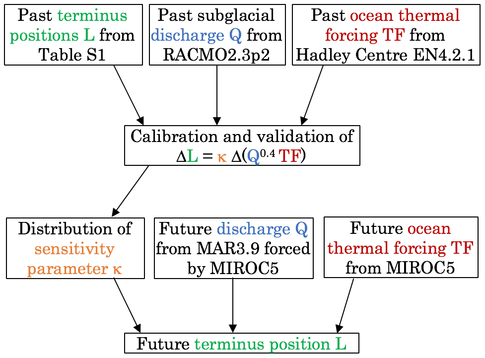
Figure 1 Schematic of approach taken in this study. We use observations and reconstructions of past terminus position, subglacial discharge and ocean temperature to calibrate and validate a simple parameterization for tidewater glacier retreat. We use the resulting parameterization, together with projections of future subglacial discharge and ocean temperature, to project future terminus position.

We develop and test our parameterization as follows. First, past observations or reconstructions of terminus positions, subglacial discharge and ocean temperatures are used to validate and calibrate the parameterization (Fig. 1). These observations span the time period 1960–2018. While we do have terminus position records from well before 1960, the subsurface ocean data coverage pre-1960 is very limited, so that we considered our estimates of ocean thermal forcing to be reliable only post-1960. In order to reduce the temporal bias in the dataset (i.e., more recent years having more terminus positions) and to bring all datasets onto a common time axis, throughout this paper we consider the mean terminus position, subglacial discharge and ocean thermal forcing over 5-year time periods. This also acts as a form of low-pass filter, removing short-term variability, which is not important to the longer-term trends that we aim to capture. Our results are not sensitive to the length of the binning period (Fig. S7 in the Supplement), although the data record is too short for much longer binning periods. Following this exercise, which provides a probabilistic range of values of the sensitivity parameter κ, future glacier retreat can be projected with the use of climate model output to estimate the right-hand side of the parameterization (Fig. 1).

2.2 Past observations

2.2.1 Terminus positions

Terminus positions are taken from a number of published sources (Fig. 2, Table S1 in the Supplement, Andresen et al., 2012; Steiger et al., 2018; Lea et al., 2014; Haubner et al., 2018; Catania et al., 2018; Cowton et al., 2018; Moon and Joughin, 2008; Joughin et al., 2018; Bunce et al., 2018; Carr et al., 2017). Broadly, these records can be organized into long records from a handful of individual glaciers and shorter satellite-era records from almost all of the fastest-flowing tidewater glaciers in Greenland (Fig. 2a and b). Thus, the number of records from before 1992 is rather limited, while coverage from the year 2000 is nearly complete (Fig. 2c). In total the dataset includes 191 of the 211 fastest-flowing tidewater glaciers in Greenland identified by Rignot and Mouginot (2012). We believe that the records we have collated constitute the most complete such dataset to date. We removed three glaciers known to have persistent ice shelves (Petermann, Ryder and 79 N) as the dynamics of ice shelf fronts differ from grounded tidewater glaciers fronts, but we retained other glaciers that may have had a floating terminus for part of the study period (e.g., Jakobshavn). Since ice tongue break-up likely occurs faster than grounding line retreat (Holland et al., 2008), the inclusion of these data could in theory lead to a larger value of κ than would otherwise be obtained, but we do not believe this issue affects a substantial number of glaciers and therefore will not influence our conclusions.

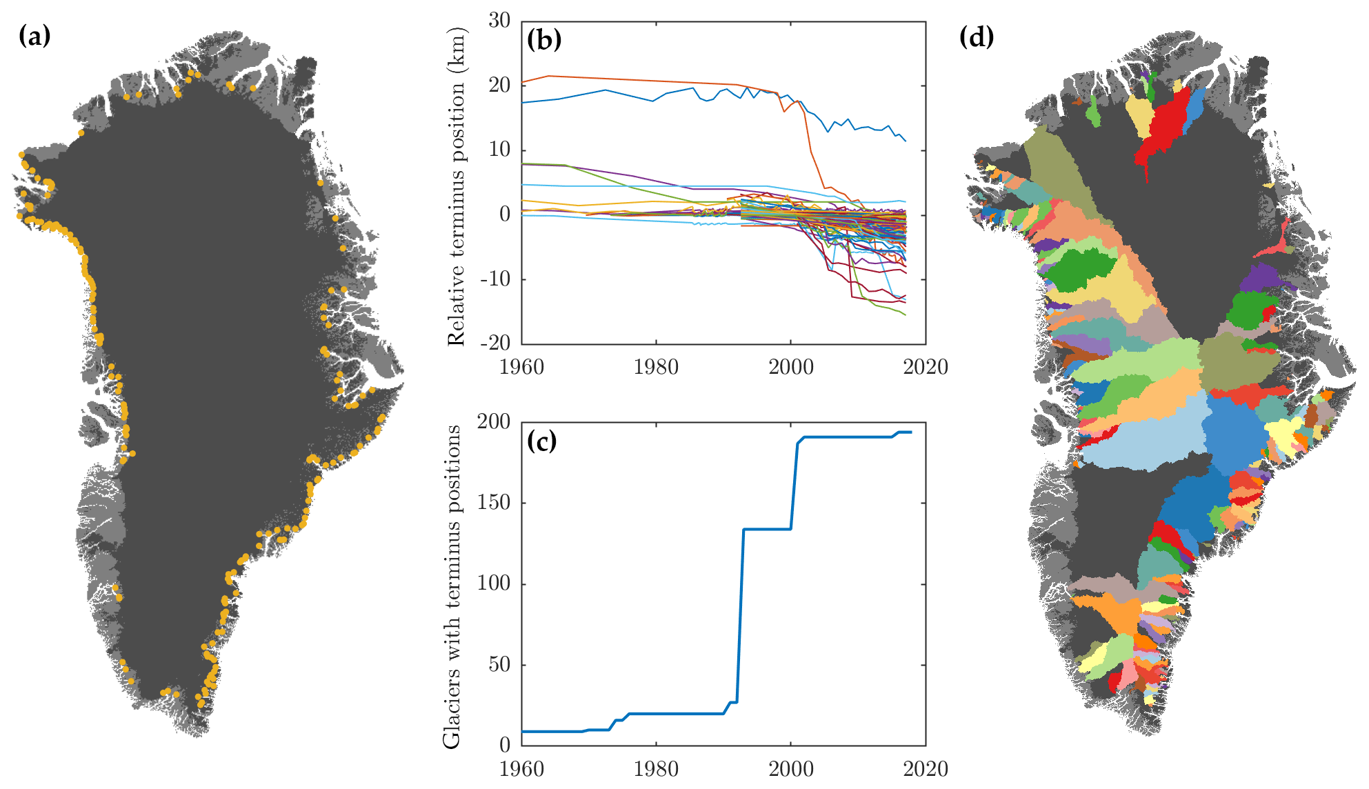
Figure 2 (a) Locations of tidewater glaciers considered, (b) overview of terminus position change at all glaciers, (c) number of glaciers in the dataset as a function of time and (d) hydrological drainage basins for each of the 191 tidewater glaciers in the terminus position dataset, calculated using hydrological flow routing with topography from BedMachine version 3 (Morlighem et al., 2017).

2.2.2 Subglacial discharge

Subglacial discharge for each of the 191 tidewater glaciers is estimated using the regional climate model RACMO (Noël et al., 2018). The surface runoff dataset is statistically downscaled to 1 km from the output of RACMO2.3p2 at 5.5 km horizontal resolution. Compared to the data discussed in Noël et al. (2018), no model physics have been changed. Refined horizontal resolution of the host model, i.e., 5.5 km instead of 11 km, better resolves gradients in SMB components at the ice sheet margins. The simulation is forced at its boundaries by ERA-40 and ERA-Interim and spans the full time period 1960–2018 considered here. Similar simulations using MAR (Fettweis et al., 2017) showed only insignificant differences.

Surface runoff is assumed to access the bed of the ice sheet and to emerge from the glacier grounding line instantaneously as subglacial discharge. It is routed to the ice sheet margins based on the subglacial hydrological potential (Shreve, 1972; Schwanghart and Scherler, 2014). We take surface and bed topography from BedMachine version 3 (Morlighem et al., 2017; Howat et al., 2014) and assume that subglacial water pressure is equal to ice overburden pressure. This process defines a hydrological basin for each tidewater glacier (Fig. 2d), over which surface runoff from the regional climate model is summed to give an estimated subglacial discharge for the tidewater glacier. We assume that the drainage basin is fixed in time. Throughout this paper, we apply a single value of subglacial discharge per glacier per year as at no point in the analysis do we consider timescales shorter than 1 year. Given the strong seasonality in subglacial discharge and since most tidewater glacier retreat is observed to take place during the summer (Fried et al., 2018), the single value of subglacial discharge is taken to be the mean summer subglacial discharge over June, July and August. An analysis of the relationship between annual and summer subglacial discharge (Fig. S3) indicates that no significant differences in results or projections would arise from using annual mean discharge rather than summer mean discharge.

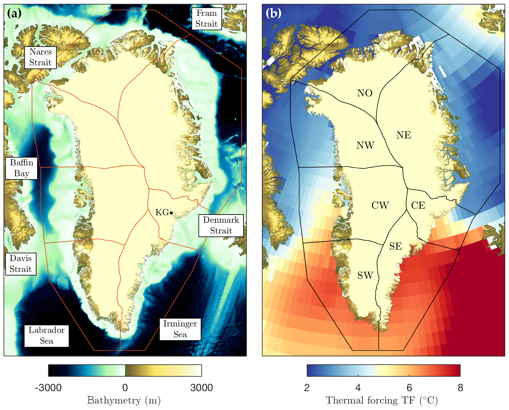
Figure 3 (a) Ocean bathymetry around Greenland (Schaffer and Timmermann, 2016) and (b) 200–500 m depth-average, 1995–2014 time-averaged thermal forcing around Greenland from the EN4 dataset (Good et al., 2013). Red lines in (a) and black lines in (b) show the ice–ocean sectors over which the thermal forcing is averaged. The location of key geographic features mentioned in the text are shown in (a) with “KG” indicating Kangerdlugssuaq Glacier, while the ice–ocean sectors are labeled in (b).

2.2.3 Ocean temperature

Subsurface ocean temperatures around Greenland (Fig. 3) come from the Hadley Centre EN4 dataset version 4.2.1 (Good et al., 2013). Alternative datasets, such as the World Ocean Atlas, or alternative methods, such as ocean reanalysis (e.g., Yang et al., 2017), do not differ significantly from EN4. We use the EN4 monthly objective analyses, which is a 1^∘ latitude by 1^∘ longitude gridded product of temperature and salinity formed from oceanographic profiles. The dataset covers the period 1900 to 2018 at monthly intervals, though profile data are limited in the early part of the time series and in the northern half of Greenland, so that as already described we only consider the time period 1960–2018. An overview of the spatial and temporal coverage of profile data going into the gridded ocean product is shown in Figs. S4 and S5. Ocean thermal forcing is defined as $\mathrm{TF}=T-T_{\mathrm{f}}$, where T is the in situ temperature and T_f the in situ freezing point. Here we use a common linear expression for the freezing point (Jenkins, 2011) to estimate thermal forcing as $\mathrm{TF}=\mathit{\theta }-({\mathit{\lambda }}_{\mathrm{1}}S+{\mathit{\lambda }}_{\mathrm{2}}+{\mathit{\lambda }}_{\mathrm{3}}z)$, where θ is potential temperature, S is practical salinity, z is depth and λ values are as in Jenkins (2011). Note that in situ and potential temperature differ by no more than 0.04 ^∘C for the depths and ocean conditions considered here.

The ocean forcing felt by tidewater glaciers is related to, but not the same as, the ocean forcing available on the continental shelf and in the ocean basins around Greenland. In particular, offshore warm deep waters and their seasonal cycle are modified by fjord circulation processes before reaching calving fronts (Straneo et al., 2011; Mortensen et al., 2011; Jackson et al., 2014; Gladish et al., 2015b). While rapid progress has been made in understanding fjord circulation and in mapping fjord bathymetry, we as yet lack the simple parameterizations and complete datasets required to include fjord effects in this study. As such, we here depth-average the thermal forcing between 200 and 500 m, this being the characteristic grounding line depth range of Greenlandic tidewater glaciers (Morlighem et al., 2017). We also average over each year and spatially average over defined sectors (Fig. 3) to give a thermal forcing (TF) per year and per sector to be used as a proxy for the thermal forcing felt by tidewater glaciers. The use of sector averages means that every glacier in a given sector experiences the same thermal forcing and is justified at present by the sparsity of oceanographic data available around Greenland and our inability to account for the effect of individual fjords.

Sectors are chosen as a compromise between oceanic basins (Fig. 3a), ocean temperature gradients (Fig. 3b) and ice sheet drainage basins, where the boundaries are similar to previous studies (Shepherd et al., 2012; Mouginot et al., 2019). We thus have sector boundaries over Davis Strait, Nares Strait and Fram Strait, and we separate the Irminger Sea from the Labrador Sea with a boundary close to Cape Farewell (Fig. 3a). We separate western Greenland from northwestern Greenland due to the large meridional temperature gradient in Baffin Bay (Fig. 3b). Finally, we create a small central eastern Greenland sector, which includes the whole Denmark Strait region; from the ocean perspective it would be desirable to instead place a sector boundary on the Denmark Strait, but extending this boundary onto the ice sheet is awkward due to the presence of Kangerdlugssuaq Glacier. We extended the ocean sectors beyond the continental shelf towards the center of the ocean basins because oceanographic data coverage improves significantly beyond the shelf (Figs. S4 and S5); we note, however, that the thermal forcing obtained is not sensitive to the exact definition of this boundary.

2.3 Future climate forcing

To generate projections of 21st century terminus position (Fig. 1), we use the global climate model MIROC5 (Watanabe et al., 2010) to estimate future ocean thermal forcing and output from the regional climate model MAR (Fettweis et al., 2013) forced by MIROC5 to estimate future subglacial discharge. Both low (RCP2.6) and high (RCP8.5) greenhouse gas emissions scenarios are considered. We emphasize that these projections are intended as an illustration for a single model rather than a rigorous result, as global climate models can differ significantly in their projected ocean and atmospheric warming (e.g., Yin et al., 2011). We also note that these emissions scenario simulations do not capture past climate variability and so cannot be used in the calibration of the parameterization.

Ice sheet surface mass balance is generally included in only a basic manner in global climate models, including MIROC5, and we therefore estimate future subglacial discharge Q using 1950–2100 simulations in the regional climate model MAR, forced at its boundaries by MIROC5 (Fettweis et al., 2013). With respect to MAR simulations performed in Fettweis et al. (2013), the latest version of MAR (3.9.6) is used here at a resolution of 15 km. The outputs were furthermore downscaled to 1 km to better account for sub-grid-scale topography (Franco et al., 2012; Howat et al., 2014). Finally it should be noted that the MAR simulations use a fixed present-day topography that is acceptable to 2100 according to Le clec'h et al. (2019). Surface melting from MAR is summed over each of the tidewater glacier drainage basins (Fig. 2d) to give a subglacial discharge time series for each glacier extending to 2100. Future thermal forcing is obtained directly from MIROC5 output by following the same procedure as for the observations: we convert potential temperature to thermal forcing, we average the model output over each year, over the depth range 200–500 m, and spatially over the ice–ocean sectors (Fig. 3). The time series are adjusted to eliminate systematic offsets during the period of overlap with past subglacial discharge from RACMO and past thermal forcing from EN4, ensuring the transition from past to future climate forcing is continuous (Appendix A).

2.4 Statistics

We assess the statistical significance of relationships between 5-year binned terminus position and parameterized submarine melt rate as follows. Since trends exist in both time series, which could lead to spurious correlation, the time series are first detrended (Fig. S6) by subtracting a linear trend in time over the full length of the dataset (Santer et al., 2000; Hanna et al., 2013). Linear regression is then performed on the detrended time series to obtain a linear coefficient b and standard error s_b (Fig. S6). We test whether b is significantly different from 0 by forming the ratio τ_b = b∕s_b and performing a two-sided t test on τ_b with N degrees of freedom. To account for temporal autocorrelation in the time series, we reduce the degrees of freedom by defining $N=n(\mathrm{1}-r_{\mathrm{1}}{r}_{\mathrm{2}})/(\mathrm{1}+r_{\mathrm{1}}{r}_{\mathrm{2}})$, where n is the number of values in the time series and r₁ and r₂ are the lag one autocorrelation coefficients for the terminus position and submarine melt time series (Santer et al., 2000; Hanna et al., 2013). If, following this procedure, we find b to be significantly different from 0 (say at the 5 % level), this implies a significant relationship between terminus position and submarine melt. In this study we apply this procedure to assess significance at both an individual glacier and Greenland-wide level.

Note that while we assess statistical significance using detrended time series, we assess the sensitivity κ of terminus position to submarine melt using the original (trended) time series. We consider this necessary because we wish to ensure that the parameterization in Eq. (1) captures past behavior of tidewater glaciers in Greenland as closely as possible and because there is strong process evidence linking increased submarine melting to tidewater glacier retreat. Thus, values of κ and correlation coefficients R² are calculated using the original time series, as we wish to give an indication of how well Eq. (1) captures past behavior, but values of statistical significance p are calculated using detrended time series and reduced degrees of freedom, as described above and illustrated in Fig. S6.

3 Results

3.1 Relationship between submarine melting and terminus position

We begin our analysis by examining two glaciers, Kangiata Nunata Sermia in southwestern Greenland and Store Glacier in central western Greenland, which exemplify the diversity of glacier response to submarine melting (Fig. 4). The terminus of Kangiata Nunata Sermia was stable within ±500 m from 1960 until 2000, before undergoing a rapid retreat of 2 km followed by restabilization (Fig. 4a). Subglacial discharge has increased steadily since 1980 (Fig. 4b), while southwestern Greenland ocean temperatures have warmed since 1995 after approximately 20 years of colder conditions (Fig. 4c). Submarine melting (Fig. 4d), combining subglacial discharge and thermal forcing, was stable from 1960 to 1995 before a rapid increase until 2010 and a small decrease since. Lastly we define anomalies of terminus position and submarine melting as the difference from their respective means over their common time period. Note that the precise definition of this anomaly is not important because it does not affect the slope of best fit (κ) nor the statistics, but the chosen definition allows us to compare different glaciers on the same axes. By considering the relationship between terminus position anomaly and submarine melting anomaly (Fig. 4e) we find a statistically significant relationship between terminus position and submarine melt rate (p=0.01) with variability in submarine melting explaining 83 % of terminus position change and a sensitivity coefficient $\mathit{\kappa }=-\mathrm{0.11}$.

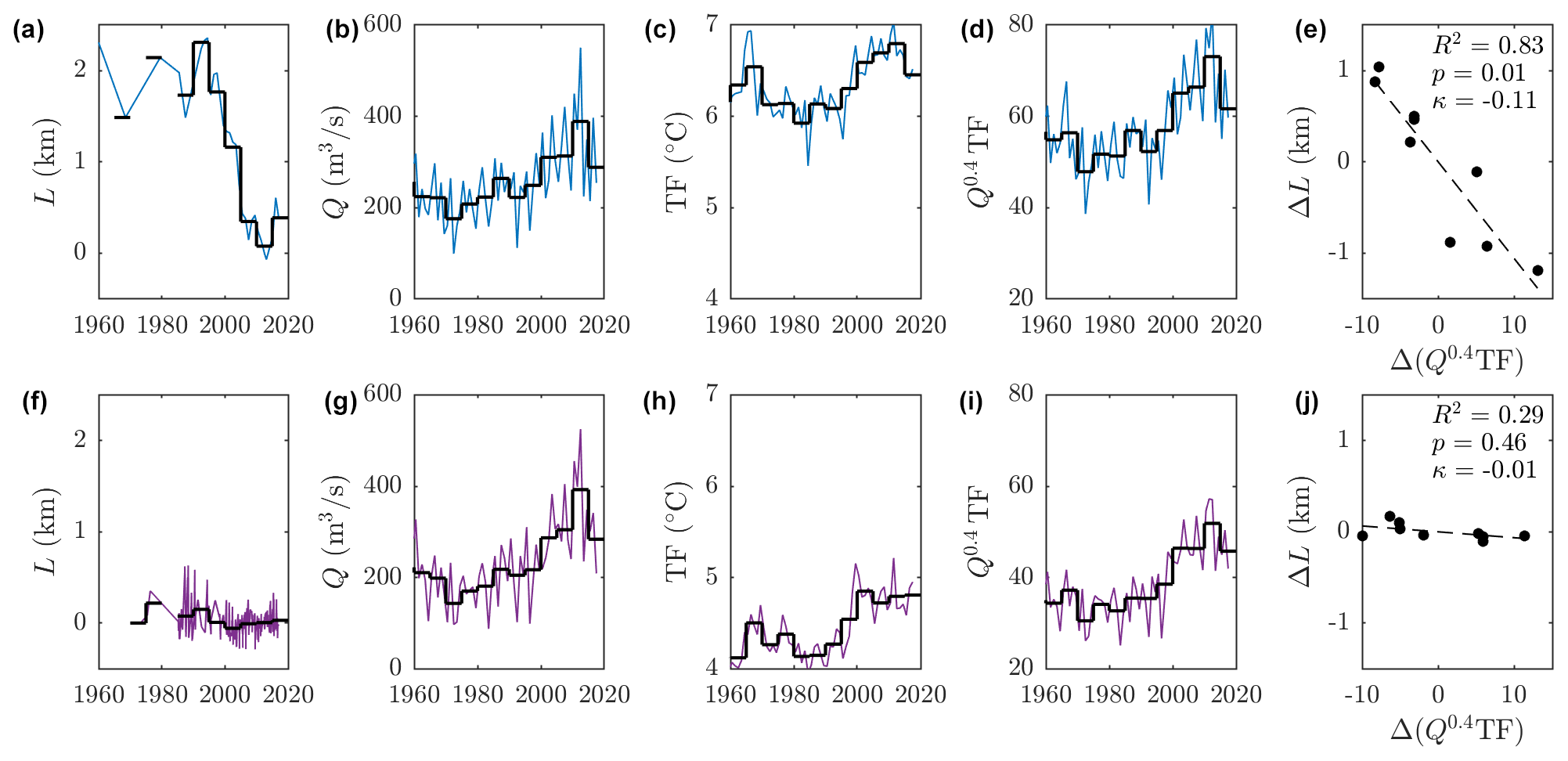
Figure 4 Example calibration of the retreat parameterization for two glaciers: Kangiata Nunata Sermia in southwestern Greenland (top row) and Store glacier in central western Greenland (bottom row). (a, f) Terminus position, (b, g) summer subglacial discharge, (c, h) ocean thermal forcing and (d, i) parameterized submarine melting. Light lines show all values in the datasets, while the heavy black lines show 5-year binning. (e, j) The 5-year binned values of parameterized submarine melt anomaly (x axis) versus terminus position anomaly (y axis). The text in (e) and (j) shows the correlation coefficient (R²), the significance of the regression (p) and the linear coefficient (κ).

Store Glacier has, in contrast, remained stable since at least 1970, with a very moderate retreat of a few hundred meters in the 1990s (Fig. 4f). Subglacial discharge has also increased steadily until the past few years (Fig. 4g), and ocean temperatures in CW Greenland show an increasing trend throughout most of the period (Fig. 4h). Estimated variability in submarine melting (Fig. 4i) explains only 29 % of terminus position change (Fig. 4j). The estimated sensitivity coefficient is $\mathit{\kappa }=-\mathrm{0.01}$, suggesting that Store Glacier is relatively insensitive to submarine melting, a conclusion previously attributed to the particular bed topography of the glacier (Morlighem et al., 2016; Todd et al., 2018). Therefore, unsurprisingly, the relationship between submarine melting and terminus position is not found to be significant at Store Glacier.

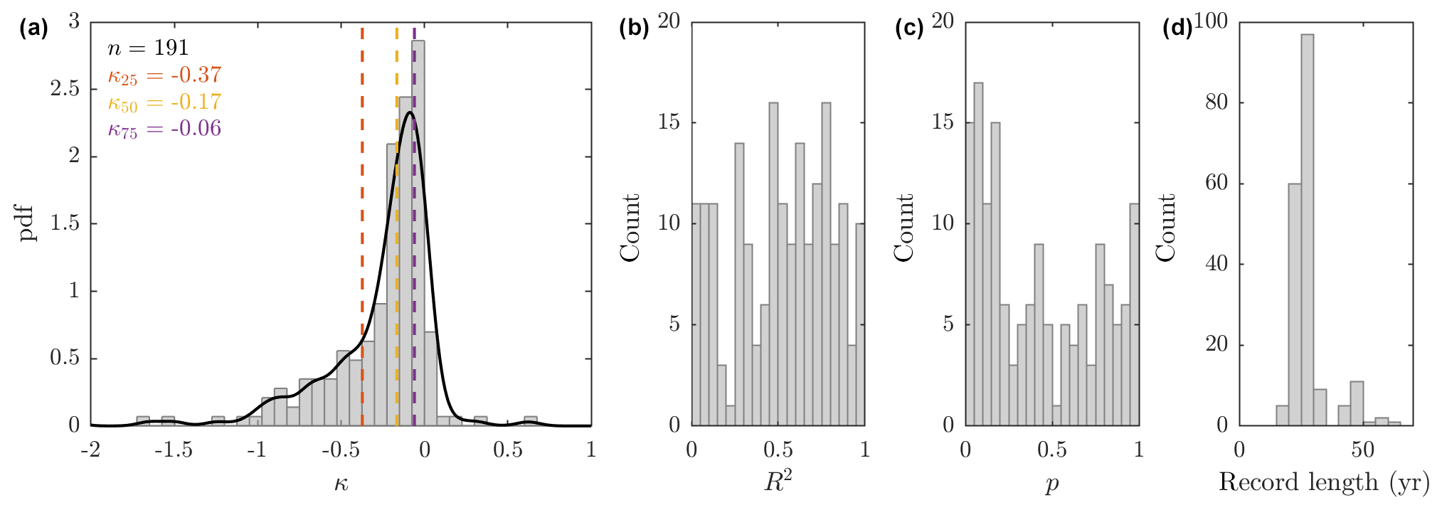
Figure 5 Result of linear regression (as in Fig. 4e and j) for all glaciers. Histograms of (a) sensitivity coefficient κ, (b) correlation coefficient R², (c) statistical significance p and (d) length of record entering the regression. Vertical dashed lines on (a) indicate the quartiles of the distribution, while the solid black line shows a kernel distribution fit to the histogram. Glaciers with a record of length less than 15 years were excluded from all plots.

This procedure can be repeated for every glacier around the ice sheet (Fig. 5). The sensitivity coefficient κ relating submarine melt forcing to change in terminus position forms a skewed distribution with very few positive κ values (increased submarine melting associated with glacier advance) and a long tail of negative κ values (Fig. 5a). The sharply peaked distribution suggests that many glaciers in Greenland show similar order-of-magnitude sensitivity to submarine melting. The median value is ${\mathit{\kappa }}_{\mathrm{50}}=-\mathrm{0.17}$, while the lower and upper quartiles take values ${\mathit{\kappa }}_{\mathrm{25}}=-\mathrm{0.37}$ and ${\mathit{\kappa }}_{\mathrm{75}}=-\mathrm{0.06}$, respectively. Kangiata Nunata Sermia, with $\mathit{\kappa }=-\mathrm{0.11}$ (Fig. 4e), therefore shows fairly average sensitivity to submarine melting, while Store Glacier with $\mathit{\kappa }=-\mathrm{0.01}$ (Fig. 4j) is more insensitive than 90 % of glaciers in Greenland. Variability in submarine melting explains greater than 50 % of the terminus position change at 105 glaciers (Fig. 5b), but the relationship is statistically significant at the 5 % level at only 15 glaciers (Fig. 5c). Finally, although we do have several glaciers for which the regression is performed on a record longer than 50 years, for the majority of glaciers the length of record is less than 30 years (Fig. 5d). This results from a combination of lack of terminus positions before the satellite era and the sparsity of ocean data until the past few decades.

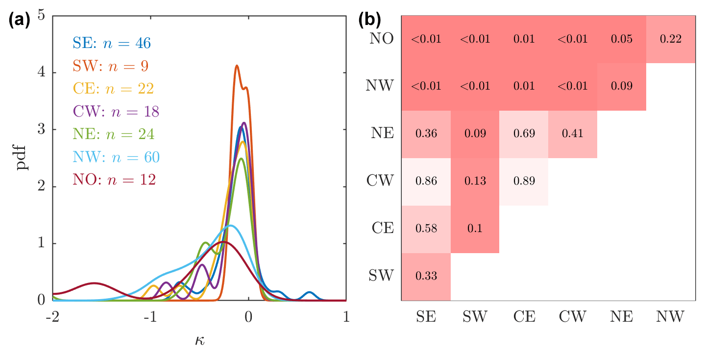
Figure 6 Sector-to-sector differences in sensitivity of glaciers to submarine melting. (a) Equivalent of Fig. 5a by ice sheet sector, where n indicates the number of glaciers entering the probability density function. (b) The p value obtained from a two-sample Kolmogorov–Smirnov test to determine significance of differences between sectors. A value p<0.05 indicates a significant difference between sector distributions in (a) and thus a significant difference in sector sensitivity to submarine melting.

We examine sector-to-sector variability in sensitivity to submarine melting by conducting the same analysis for each sector separately (Fig. 6). The five more southerly and easterly sectors (SE, SW, CE, CW and NE; see Fig. 3b) show remarkably similar sensitivity of terminus position to submarine melting, as indicated by similar distributions for κ (Fig. 6a). The most northerly and westerly sectors (NW and NO) show distributions with peaks shifted to more negative κ values and have longer tails reaching out to larger negative κ values, indicating that these sectors show higher sensitivity of terminus position to submarine melting. We test whether the sector-specific κ distributions are significantly different using a two-sample Kolmogorov–Smirnov test (Fig. 6b). At the 5 % level, the far north sector (NO) is indeed statistically different to all sectors except the northwest (NW), while the NW sector is statistically different to all sectors except the far north (NO) and northeast (NE).

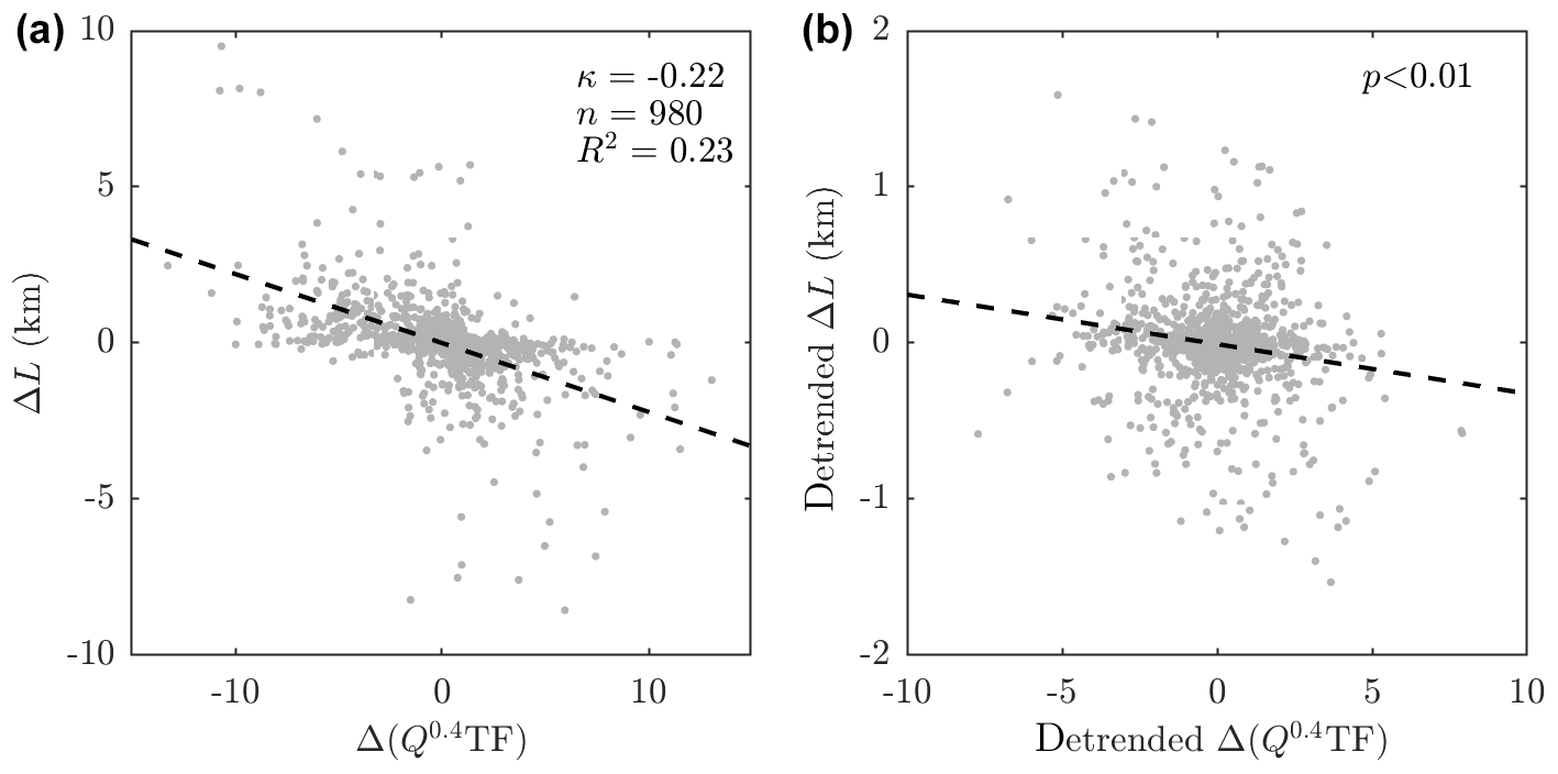
Figure 7 (a) Correlation of submarine melt anomaly versus terminus position anomaly for all glaciers. Each light grey point is a 5-year binned value for an individual glacier. The dashed black line is linear regression on the scatter, and statistics are given in the top right. Panel (b) is the same as panel (a), but a linear trend in time for each glacier has been removed from both the submarine melt and terminus position, outliers have been removed, and the p value also accounts for autocorrelation (Sect. 2.4).

Considering all glaciers together by plotting 5-year binned terminus position anomaly versus submarine melt anomaly, with anomalies again calculated as the difference from the mean, variability in submarine melting explains 23 % of change in terminus position over all glaciers with a best fit linear coefficient $\mathit{\kappa }=-\mathrm{0.22}$ (Fig. 7a). Since p<0.01, the relationship between terminus position and submarine melting is statistically significant after detrending and accounting for autocorrelation and remains so if points lying more than 2 standard deviations from the trend line are removed (Fig. 7b).

Our analysis therefore shows that there is a statistically significant relationship between submarine melting and terminus position at the ice sheet scale and at a minority of individual glaciers. Similarly, the proposed retreat parameterization is able to explain a substantial portion of observed terminus position change at the ice sheet scale and at a majority of individual glaciers. Together with process understanding linking submarine melting to glacier dynamics, this analysis supports our proposed parameterization. We note, however, the substantial proportion of terminus position change, which is not explained by submarine melting (77 % at the ice sheet scale, Fig. 7a), and the wide range of observed glacier sensitivity to submarine melting at both individual and regional levels (Figs. 5a and 6a). As such, we expect that the proposed retreat parameterization should be able to predict the magnitude of retreat of a population of glaciers in response to climate change but may perform poorly at an individual glacier level.

3.2 Validation of the retreat parameterization

Given the observed sensitivity of tidewater glaciers to submarine melting (Fig. 5a), there are a couple of ways in which the retreat parameterization Eq. (1) could be employed. One method would be to project retreat for each glacier using the specific value of κ obtained from the history of that glacier. Thus, for Kangiata Nunata Sermia we would use $\mathit{\kappa }=-\mathrm{0.11}$ (Fig. 4e) and for Store Glacier we would use $\mathit{\kappa }=-\mathrm{0.01}$ (Fig. 4j). Under this approach we would be conditioning each glacier to behave in a similar fashion as it has in the past, so that Kangiata Nunata Sermia would retreat significantly under an increase in submarine melt, while Store Glacier would retreat only slightly. This approach might be considered desirable in some circumstances for some time period. For example, it is thought unlikely that Store Glacier will retreat significantly in the next few decades (Morlighem et al., 2016).

In general, however, we do not think this is the best approach for centennial timescale projections due to the individuality and intermittency of glacier response to climate. A certain glacier might appear highly sensitive to melting (with a corresponding high value of $\left|\mathit{\kappa }\right|$) because it has retreated through an overdeepening during the period of observation. It might now have stabilized on a bed rock ridge, so that retreat over the next few decades will be much slower than in the recent past, and the high value of $\left|\mathit{\kappa }\right|$ would therefore overpredict retreat. Equally, Store glacier may at some point over the next century begin rapid retreat, but if we tune the parameterization to its past behavior this will not be projected. Similarly, one could consider employing a sector-specific value for κ (Fig. 6a), but this suffers from similar limitations. The value of κ becomes more influenced by individual glaciers as the training dataset shrinks (SW has only 9 glaciers and NO has only 12), and thus the future projections become heavily influenced by how individual glaciers have behaved in the past.

Here, we view the distribution of κ as a property of the population of tidewater glaciers in Greenland, encompassing the diversity of glacier behavior and response to climate over the recent past and over the full ice sheet. If we were to apply the retreat parameterization Eq. (1) with κ sampled from the distribution shown in Fig. 5a, then we are conditioning a glacier to behave in the future as the population of glaciers has in the past, rather than as that individual glacier has in the past. In this way we capture the possibility that a glacier will be rather insensitive to climate forcing (because some other glaciers in Greenland experiencing similar climate forcing in the past have retreated only slightly) and the possibility that it will be very sensitive (because some other glaciers have retreated dramatically under similar forcing).

Under the described sampling approach, we cross-validate the parameterization by separating the dataset into training data, on which the parameterization is calibrated as in Fig. 5a, and test data, on which we test the calibration. This allows the parameterization to be evaluated by seeing how well it captures observations of retreat when these observations have not been used to calibrate the parameterization. We consider retreat between 1995–2005 and 2005–2015 as this time period is well covered by observations (Fig. 2c). We calculate the mean terminus position in observations for the two time periods and take the difference to give an observed retreat. We project retreat by sampling κ from its distribution and, according to Eq. (1), multiplying by the difference in submarine melting between the two time periods. Since Eq. (1) is linear in κ, the distribution of projected retreat is the distribution for κ, scaled by the submarine melting anomaly.

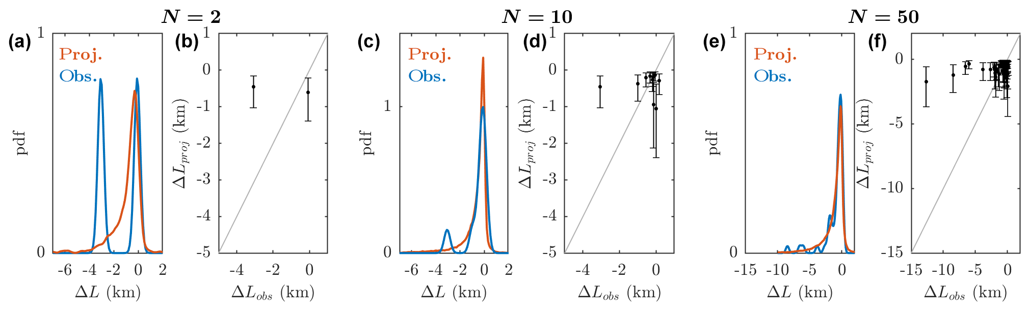
Figure 8 Validation of retreat parameterization on the observed terminus position change between 1995–2005 and 2005–2015. Note that ΔL<0 indicates retreat. In (a) and (b) we select two glaciers at random to be the test dataset and calculate the distribution for κ (as in Fig. 5a) based on all of the remaining glaciers. As described in the text we use the distribution for κ to generate projected retreat. In (a) we compare the distributions of observed (blue) and projected (red) retreat. In (b) we plot observed versus projected retreat, where the projection uses the median and interquartile range of the κ distribution. Panels (c) and (d) are the same but select 10 glaciers at random, while (e) and (f) select 50 glaciers at random.

The result of this procedure for varying choices of training and test data is shown in Fig. 8. We consider first a test dataset of 2 randomly chosen glaciers, leaving 189 glaciers in the training dataset. The distributions of observed and projected retreat are shown in Fig. 8a (we obtain the observed distribution as a kernel distribution with bandwidth 0.25 km). It is clear that the two distributions do not agree well, a fact which is further illustrated in Fig. 8b – the retreat parameterization significantly underestimates retreat for one of the glaciers and slightly overestimates retreat for the other. Increasing the size of the test dataset to 10 randomly chosen glaciers (leaving 181 in the training dataset) results in an improved agreement between observations and projections, illustrated by increased overlap in the observed and projected distributions (Fig. 8c and d). Once the size of the test dataset is increased to 50, agreement between the observed and projected distributions is very good. There remain individual glaciers for which the parameterization performs poorly (Fig. 8f), but the distributions are in very good agreement (Fig. 8e).

These exercises validate the application of the retreat parameterization when κ is sampled from its distribution. They show that given a sufficiently large dataset on which to calibrate the parameterization, we are able to successfully predict the retreat of a population of glaciers (Fig. 8e and f). Although this sampling approach results in a large range of projected retreat for each individual glacier, it is more honest to the diversity of glacier response than using a single value of κ for each glacier. Having justified, calibrated and validated the retreat parameterization, we now proceed to project retreat over the 21st century.

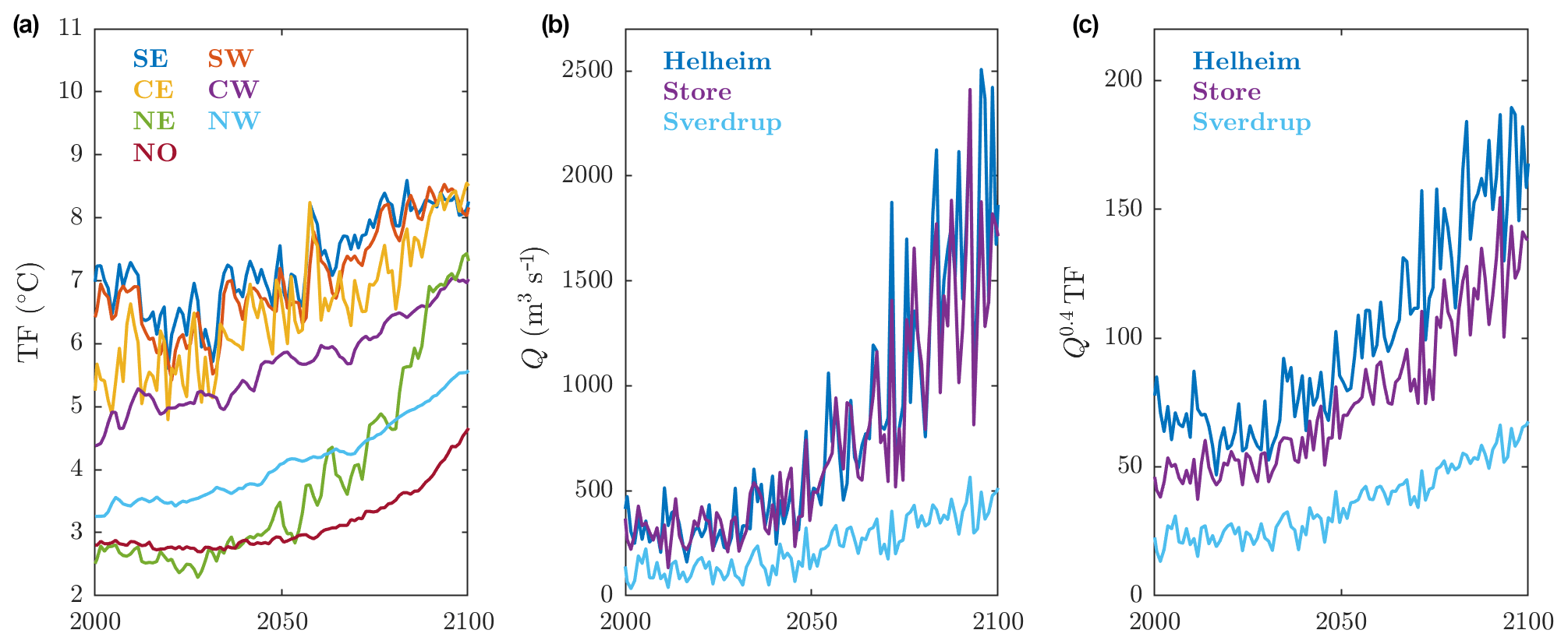
Figure 9 Projected RCP8.5 tidewater glacier climate forcing using the climate model MIROC5 and regional climate model MAR. (a) Thermal forcing (TF) from MIROC5 for each of the ice–ocean sectors. (b) Subglacial discharge (Q) for selected glaciers from a MAR simulation forced by MIROC5. (c) Parameterized submarine melting. The colors in (b) and (c) show the ice–ocean region to which the glacier belongs.

3.3 Projected 21st century tidewater glacier retreat

To demonstrate the use of the parameterization we consider projected tidewater glacier terminus position change over the 21st century under RCP2.6 and RCP8.5 scenarios in the climate model MIROC5 (Watanabe et al., 2010). To illustrate the procedure and to highlight spatial variability, we consider three example glaciers (Fig. 9) but once more emphasize the parameterization is more suited to groups of glaciers, which are considered last of all.

All ice–ocean sectors show significant ocean warming in the MIROC5 RCP8.5 simulation (Fig. 9a), though there is spatial variability with the far north (NO) showing the least warming by the end of the century (1.7 ^∘C) and the northeast (NE) showing the most warming (3.9 ^∘C), more than doubling the thermal forcing in this sector. Three example glaciers also show significant increases in subglacial discharge by the end of the century (Fig. 9b). Subglacial discharge at Helheim glacier in southeastern Greenland, averaging ∼300 m³ s⁻¹ during 1995–2014, increases to ∼1750 m³ s⁻¹ during 2081–2100, an increase of approximately a factor of 6. Making the same comparison for Store and Sverdrup glaciers, subglacial discharge increases by a factor of 5 and 3.5, respectively. Future submarine melt forcing, estimated as Q^0.4 TF, increases by a factor of 2 to 3 by the end of the century in an RCP8.5 scenario (Fig. 9c). In contrast, the climate forcing experienced by tidewater glaciers is projected to change comparatively little under a low greenhouse gas emissions scenario RCP2.6 (Fig. S8).

Tidewater glacier retreat is then estimated by combining the submarine melt forcing for each glacier with the distribution of glacier sensitivity κ. Specifically, and as motivated in Sect. 3.2, we randomly sample 10⁴ values of κ from the distribution (Fig. 5a) and project retreat by multiplying by the Q^0.4 TF time series for the glacier in question (e.g., Fig. 9c). The κ values are taken to be constant in time. This yields 10⁴ retreat projections for each glacier. Retreat is assumed to stop once the glacier becomes land-terminating, as once this happens retreat will be much slower and no longer controlled by submarine melting. For some glaciers this is within 5 km of retreat while others can retreat hundreds of kilometers before becoming land-terminating (Fig. S9). We choose to reference our retreat to the year 2014; thus, we set L=0 in 2014 for all glaciers, and any projected change ΔL is to be understood as relative to this baseline. Finally, we do not expect tidewater glaciers would respond sufficiently rapidly to capture the high interannual variability in the climate forcing, and we therefore smooth the projections using a centered 20-year moving average. Although this is a longer smoothing interval than the 5-year binning applied to the calibration datasets, it targets the century-scale trend, which is the focus of this paper and current ice sheet modeling efforts.

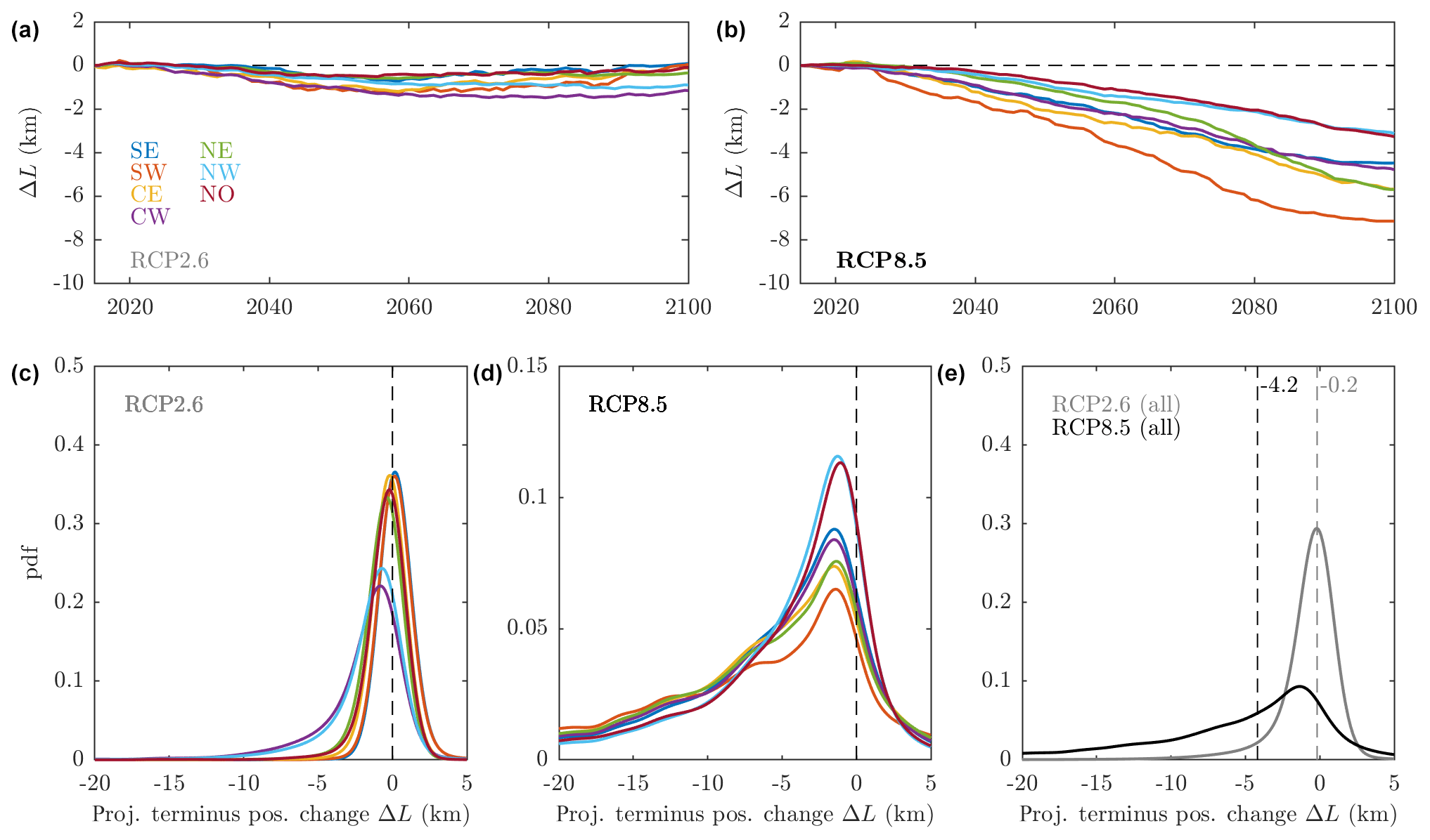
Figure 10 Projected tidewater glacier terminus position change by sector as forced by the climate model MIROC5. (a, b) Time series of median retreat by sector under (a) an RCP2.6 scenario and (b) an RCP8.5 scenario. (c–e) Probability distributions for tidewater glacier terminus position change by 2100. Panel (c) shows the RCP2.6 scenario by sector, panel (d) shows the RCP8.5 scenario by sector, while panel (e) shows full ice sheet distributions for both RCP2.6 and RCP8.5. Colors in (b)–(d) are the same as for the legend in (a). The vertical dashed lines and number labels in (e) indicate the median retreat in kilometers for each emissions scenario.

We then repeat this procedure for each of the 191 glaciers in our dataset and group the glaciers by ice–ocean sector to give projected terminus position change for each sector under both RCP2.6 and RCP8.5 scenarios (Fig. 10). Under an RCP2.6 scenario, the projections show limited retreat until 2060 for all sectors before stabilization or readvance (Fig. 10). Probability distributions of projected change by 2100 are tightly clustered around 0 because MIROC5 predicts little warming of the ocean or atmosphere in an RCP2.6 scenario (Figs. 10c and S8). For most regions, glacier advance (ΔL>0) is as probable as retreat, while in the CW and NW sectors retreat is more probable because MIROC5 does predict significant warming of the ocean in these regions (Fig. S8).

Under an RCP8.5 scenario, substantial retreat is projected in all sectors (Fig. 10b) due to considerable increases in subglacial discharge and ocean temperature (Fig. 9). Sector-to-sector variability in the projections arises both due to regional variability in projected climate and the characteristics of glaciers in a sector, as glaciers with larger hydrological basins tend to retreat further under our parameterization. Retreat is therefore largest for the SW sector because this sector has a small number of glaciers with relatively large basins, while the NW sector has a large number of glaciers with smaller basins. Considering projected retreat by 2100, the probability distributions are much broader than for RCP2.6, with a much larger retreat more probable (Fig. 10d).

At the ice sheet scale, projected terminus position change under RCP2.6 is sharply peaked around 0 with a median retreat of 0.2 km, indicating little change from present levels with a significant number of glaciers predicted to advance (Fig. 10e). Thus, under RCP2.6 we expect that 50 % of glaciers in Greenland would undergo retreat of less than 0.2 km by the end of the century. There is a not insignificant tail of retreat greater than 3 km, which is almost entirely due to significant ocean warming in the CW and NW sectors (Fig. 10a and c), though this may be specific to the climate model MIROC5 (Yin et al., 2011). Under RCP8.5 the distribution shifts leftwards and broadens significantly (Fig. 10e). The peak of the distribution still occurs at a moderate retreat of only ∼1 km because there are a large number of small tidewater glaciers in Greenland, which typically show only small response to climate forcing. The median retreat is now 4.2 km; thus, we are suggesting that 50 % of glaciers will undergo retreat exceeding 4.2 km by 2100. The distribution also suggests that retreat by 2100 will exceed 10 km for 27 % of glaciers and will exceed 20 km for 12 % of tidewater glaciers in Greenland under an RCP8.5 scenario.

4 Discussion

4.1 Philosophy and interpretation of parameterization

We have used past climate and terminus position observations and reconstructions, together with process understanding of submarine melting and tidewater glacier dynamics, to show there is a statistically significant relationship between tidewater glacier terminus position and estimated submarine melt. On this basis we have calibrated and validated a parameterization in which tidewater glacier retreat is linearly related to submarine melting. The parameterization is not intended to capture short-term glacier-to-glacier variability in retreat rate, which is likely driven by bed topography or fjord dynamics. As such the parameterization is essentially asking, given past climate and terminus position variability and projected climate warming, how much should we expect tidewater glaciers to retreat? Our strategy emphasizes distributions of retreat rather than individual glacier retreat trajectories.

Under this approach, we are assuming that glaciers respond to submarine melting in the same way in the future as they have in the past. Over long timescales this assumption may break down if glaciers retreat into very shallow water or even become land-terminating, though the latter is an effect that we take into account by no longer applying the retreat parameterization once a glacier terminus is located on land. Other ways in which glaciers might respond differently would be if their subglacial hydrology changes, which could influence basal lubrication and the distribution of plumes at their calving fronts, or if a region of glaciers retreats into an area of bedrock that is characteristically rougher than before. By parameterizing retreat only in terms of submarine melting, these factors are assumed to remain constant.

We consider the existence of a statistically significant correlation between terminus position and parameterized submarine melting to strengthen the argument for the importance of submarine melting, but it is not inconceivable that the retreat parameterization might be inadvertently accounting for other drivers of calving. For example, the structural integrity of ice mélange and sea ice, thought to be important in some locations for inhibiting calving (Amundson et al., 2010; Christoffersen et al., 2012; Moon et al., 2015), would likely be compromised by increased air temperature (and thus increased subglacial discharge Q) and increased ocean temperature (and thus increased ocean thermal forcing, TF). Furthermore, because the ocean and atmosphere are a coupled system, the time series of subglacial discharge Q and ocean thermal forcing (TF) are not necessarily independent, which further confounds the identification of the key processes driving ice sheet change.

One implication of the form we have assumed for the retreat parameterization is that the terminus position is always in equilibrium with the climate, i.e., if the climate stabilizes then the terminus position stabilizes, and there is no continuing or lagged impact from past climate. The timescale of response of tidewater glaciers to climate is an ongoing topic of research, and through binning terminus positions and climate data in 5-year intervals and smoothing projections with a 20-year moving average, we have here implicitly assumed a terminus position response timescale of 5–20 years, which is supported by the observed rapid changes at tidewater glaciers in recent decades (Straneo and Heimbach, 2013) and by theory (Robel et al., 2018). Stabilization of the terminus position does not, however, imply stabilization of mass loss because thinning can propagate up-glacier for decades after terminus retreat (Price et al., 2011) and this would be captured by an ice sheet model employing our retreat parameterization. But a slower lagged response arising, for example, from atmospheric-driven thinning propagating down-glacier to the terminus and leading to frontal retreat (Robel et al., 2018) would not be captured by our parameterization.

4.2 Use of parameterization

We envisage this retreat parameterization and projections of retreat to be of use primarily to ice sheet modelers looking to simulate ice sheet response to outlet glacier retreat. The principal advantages of the parameterization are its simplicity and context provided via empirical validation, thus the critical interaction of the ice sheet with the ocean can be represented in a manner that is informed by observations and scales to regional and ice-sheet-wide applications. Such an approach is clearly very different in character from simulations which explicitly try to resolve glacier frontal dynamics (e.g., Nick et al., 2013; Morlighem et al., 2016); indeed, terminus positions in such studies typically jump quickly from one stable position to the next, while our projections instead give gradual retreat. The rapid transition between stable positions is evident in observations (e.g., Catania et al., 2018), and certainly accurately projecting mass loss at individual glaciers and over short timescales means accurately modeling these transitions. We posit, however, that imposing gradual retreat, as suggested here (e.g., Fig. 10b) is a reasonable approach for capturing mass loss at an ice sheet scale and over multidecadal timescales, especially since the timing of rapid terminus transitions is hard to capture.

Use of a retreat parameterization does heavily parameterize tidewater glacier frontal processes, but we emphasize that it does not place any constraints on ice thickness or velocity at the ice–ocean boundary, which would still be calculated dynamically by the ice flow model. The total dynamic sea level contribution is then the sum of the ice above flotation removed by the retreat parameterization together with the inland propagation of thinning in response to retreat. The retreat parameterization described in this paper is therefore the standard approach that has been recommended to ice sheet modelers simulating the future of the Greenland ice sheet in the ISMIP6 project (Nowicki et al., 2016; Slater et al., 2019), the results of which will feed into sea level projections in the next IPCC assessment report.

4.3 Comparison to existing projections

Few studies have projected tidewater glacier retreat for comparison to our projections. Nick et al. (2013) used a flow line model to project retreat for four of Greenland's largest glaciers under an RCP8.5 scenario. We compare projections in Fig. S10; for all glaciers the projections in Nick et al. (2013) lie within the interquartile range of our projections (though we do not consider Petermann glacier here as it has a persistent ice shelf). Taking Helheim glacier as an example, Nick et al. (2013) project retreat of 17–26 km between 2014 and 2100 while in our study we project a median of 17 km and an interquartile range of 6–35 km (Fig. S10). Beckmann et al. (2019) used a similar flow line model to project retreat for 12 assorted glaciers under an RCP8.5 scenario; a comparison is shown in Fig. S11 and shows once more that – within the interquartile range – our projections agree with all 12 of those from the flow line model. Lastly, Morlighem et al. (2019) used a state of the art ice flow simulation together with dynamic modeling of frontal processes to project the future evolution of NW Greenland, but their climate forcing is not easily comparable to the RCP scenarios considered here.

Cowton et al. (2018) calibrated a retreat parameterization based on 20 years of evolution of 10 tidewater glaciers in eastern Greenland. Relative to their study, we have substantially greater spatial coverage (including 191 of the largest tidewater glaciers in Greenland) and significantly greater temporal coverage (including 126 glaciers with a record longer than 20 years). This expansion of the dataset allows us to find a statistically significant link between submarine melting and terminus position at the ice sheet scale, to generate projections for every tidewater glacier and region in Greenland and to quantify uncertainties in forward projections by sampling from a large distribution of glacier sensitivity to submarine melting. Nevertheless, if we compare RCP2.6 and RCP8.5 projections using the parameterization from this study and from Cowton et al. (2018), we find they are very similar (Fig. S12). The parameterization in Cowton et al. (2018) would predict a median retreat of 0.1 km under RCP2.6, relative to 0.2 km here (Fig. 10e), and a median retreat of 4.8 km under RCP8.5, relative to 4.2 km here (Fig. 10e).

4.4 Possible improvements

We have assumed a linear relationship between submarine melting and terminus position. While there is significant evidence linking tidewater glacier retreat to increased submarine melting (e.g., Straneo and Heimbach, 2013, and references therein), process studies do not yet indicate a simple relationship between submarine melting and calving, or submarine melting and terminus position (Benn et al., 2017b). Luckman et al. (2015) and How et al. (2019) suggest that at two glaciers in Svalbard calving is largely restricted to failure of ice that has been undercut by submarine melting, so that frontal ablation is linearly paced by submarine melting. This simple relationship may, however, be limited to glaciers where submarine melting can outpace ice flow, which is not thought to be the case for most of Greenland's larger tidewater glaciers (Carroll et al., 2016). At faster-flowing glaciers, studies have been conflicted on the importance of submarine melting (Cook et al., 2014; Krug et al., 2015; Todd et al., 2018) while other studies show a highly nonlinear response of calving to submarine melting (Benn et al., 2017a; Ma and Bassis, 2019). Given this uncertainty, we have here assumed the simplest possible linear relationship, and we indeed find that this is statistically significant (Fig. 7b). We do not, however, rule out the possibility that nonlinear relationships, or different combinations of climate forcing, possibly including additional parameters such as grounding line depth, might provide a closer relationship between forcing and retreat, ultimately feeding through to reduced uncertainty in future projections.

One could also consider a retreat parameterization based on relative, rather than absolute, change in submarine melting. It may be that the apparent increased sensitivity of glaciers in northern and northwestern Greenland to submarine melting (Fig. 6) results from initially low submarine melt rates in those regions, such that a given absolute increase in submarine melting is a larger relative increase in NO and northwestern Greenland than further south. We do, however, suspect that the formulation in terms of absolute melt rate may be key to finding a statistically significant link between submarine melting and terminus position. The absolute formulation encapsulates the fact that, in general, larger glaciers have greater potential to undergo large retreat. Equivalently, the numerous small tidewater glaciers in Greenland, which flow at speeds of a few hundred meters per year (Rignot and Mouginot, 2012), are unlikely to undergo retreat of several kilometers on short timescales. This is captured by an absolute formulation because small glaciers have small hydrological catchments, small subglacial discharge Q, small submarine melt rates and therefore limited absolute variability in submarine melt rate and projected retreat. In this sense, the subglacial discharge Q appearing in the retreat parameterization could be thought of as a “glacier size” parameter, and we speculate that this consideration of glacier size may be critical to finding significant relationships between glacier behavior and climate, which may explain why some studies have found significant relationships (Cowton et al., 2018; Porter et al., 2018; Cook et al., 2019) and others have struggled (Murray et al., 2015; Carr et al., 2017).

Another possibility would be to formulate a parameterization for frontal ablation rate rather than retreat (the two being related by retreat rate is ice velocity minus frontal ablation rate). A parameterization for frontal ablation rate might be considered preferable because then, through an ice sheet model, the ice velocity is allowed to influence the terminus position – that is, one could capture the potential feedback where retreat is stabilized due to an increase in ice velocity. We have nevertheless chosen to form a retreat parameterization for three key reasons. First, there is the pragmatic fact that a longer time series of terminus positions is available than of frontal ablation rate. The latter requires ice velocity, which is, in general, hard to obtain before 2000. Second, because we are tuning our parameterization empirically, the parameterization in some sense includes all potential feedbacks because these feedbacks will have been influencing the terminus positions which enter our calibration. Third, we note that Haubner et al. (2018) showed that by imposing externally specified terminus positions at Upernavik Isstrom, it is possible to capture dynamic mass loss of the glacier upstream, suggesting that specifying terminus position through a retreat parameterization is a feasible approach to modeling ice sheet dynamic response to climate.

As a final alternative parameterization, one could consider parameterizing dynamic thinning at the glacier terminus rather than terminus position, especially since Porter et al. (2018) have noted significant relationships between thinning rates and nearby ocean heat content. Substantial thinning has occurred around the margins of Greenland in recent decades, associated with tidewater glacier retreat (Khan et al., 2014; Csatho et al., 2014). If this thinning is a response to retreat then the thinning would be captured by an ice sheet model employing our retreat parameterization. If this dynamic thinning, however, results in further retreat, or if the thinning is instead driven by surface mass balance or by basal lubrication, then these are factors that are not explicitly accounted for by our retreat parameterization. They might be implicitly accounted for because we have tuned the parameterization to match observed retreat, and so if these processes have contributed to observed retreat, they will have affected our values of κ, but explicitly accounting for these factors could improve the present parameterization.

We assess there to be three key areas in which the current parameterization could be improved. Firstly, the importance of a handful of large glaciers to Greenland's sea level contribution (Enderlin et al., 2014) motivates the need for a retreat parameterization which performs well at an individual glacier level rather than just over a population of glaciers. This requires consideration of bed topography and we therefore place high priority on exploring simple ways of including bed topographic effects in a similar retreat parameterization to that considered in this study, stabilizing glaciers on pinning points and promoting rapid retreat through overdeepenings. Secondly, more long-term observations would be valuable for improving the calibration and validation of the parameterization. Aerial photography (Bjork et al., 2012) is a promising source of long-term terminus position records, but long-term oceanographic observations are sparse; careful use of limited historical records or reanalysis products might prove fruitful. Thirdly, while we expect that our estimates of subglacial discharge Q entering the parameterization are accurate (e.g., Langen et al., 2015; Noël et al., 2018), the thermal forcing (TF) is highly simplified and thus less certain, being based on spatial and depth averaging of ocean temperatures over the continental shelf and beyond. Through fjord dynamics and fjord–shelf exchange, thermal forcing at the calving front may differ from that on the continental shelf (e.g., Gladish et al., 2015a) and may differ at adjacent glaciers (Bartholomaus et al., 2016). There is therefore an urgent need for methods that can translate offshore ocean properties to calving front thermal forcing and a pressing need for sustained oceanographic observations with which to validate these models.

5 Conclusions

We have used surface melt output from a regional climate model, compilations of ocean temperature and records of glacier retreat to examine links between parameterized submarine melting and tidewater glacier terminus position change since 1960 for 191 of Greenland's marine-terminating glaciers. We find a statistically significant relationship between parameterized submarine melt rate and terminus position at the ice sheet scale and that variability in submarine melting can explain more than 50 % of variability in terminus position at 105 of the 191 glaciers considered.

On this basis, we develop a simple parameterization relating tidewater glacier retreat to submarine melt anomaly, providing a method of capturing the critical interaction between the ice sheet and ocean and the dynamic response of the Greenland ice sheet to tidewater glacier retreat, without the computational expense of explicitly resolving calving processes. The parameterization is weakest when applied to an individual glacier over short timescales, when glacier-specific factors such as bed topography play a dominant role in determining whether, when and how much a glacier will retreat in response to a climate forcing. The parameterization is strongest when applied to a population of glaciers, for example an ice sheet region, when it provides an envelope of projected retreat given how sensitive tidewater glaciers have collectively been to climate forcing in the recent past.

We provide example projections under low (RCP2.6) and high (RCP8.5) greenhouse gas emissions scenarios using output from a single global climate model MIROC5. Since significant variability exists between climate models (e.g., Yin et al., 2011), these projections should be considered largely as an illustration. For the low-emission scenario, tidewater glaciers show, in general, little change by the end of the century. Under the high-emission scenario, ocean thermal forcing increases by 2–4 ^∘C and subglacial discharge increases by a factor of 3–6 by 2100. In response, we project a median Greenland tidewater glacier retreat of 4.2 km and suggest that 27 % of glaciers will retreat more than 10 km and 12 % will retreat more than 20 km by the end of the century.

The analysis and parameterization described in this study forms the standard method that has been recommended to ice sheet modelers taking part in the ISMIP6 project (Nowicki et al., 2016; Slater et al., 2019), which aims to project sea level contribution from Greenland for the IPCC AR6. We believe that this simple process-motivated parameterization will prove useful for the projection of dynamic mass loss from Greenland and expect that it will be complemented by more complex approaches as our understanding and modeling of tidewater glacier dynamics continues to improve.

Appendix A: Climate model bias correction

Ideally, we would use the same model for both the calibration of the retreat parameterization from 1960 to 2018 and for the projections from 2014 to 2100. This is unfortunately not possible because the CMIP simulations that are widely used (including in ISMIP6) for climate projections under greenhouse gas emissions scenarios do not accurately capture past climate variability. Therefore, we cannot, for example, use the 1960–2018 output from MIROC5 to calibrate the retreat parameterization. For the calibration we have instead used what we consider to be our best estimates of past subglacial discharge (RACMO2.3p2) and thermal forcing (EN4).

In the absence of a model that can represent both past and present and to ensure a continuous transition from past to future climate forcing, we ensure that the subglacial discharge and thermal forcing coming from the climate model MIROC5 and MAR forced by MIROC5 are roughly correct in the present day by bias-correcting both time series. Specifically, we subtract a constant offset from both time series, which is given by comparing the time series to our best estimates of subglacial discharge and thermal forcing over the period 1995–2014. Thus, the projected forcing time series are defined as

$$\begin{array}{ll}{\displaystyle }X\left(t\right)=& {\displaystyle }{X}_{\mathrm{MIROC}\mathrm{5}}\left(t\right)-\left[X_{\mathrm{MIROC}\mathrm{5}}\left(\mathrm{1995}\text{–}\mathrm{2014}\right)\right.\\ {\displaystyle }& {\displaystyle }\left.-X_{\mathrm{BE}}\left(\mathrm{1995}\text{–}\mathrm{2014}\right)\right],\end{array}$$

where X is either subglacial discharge Q or thermal forcing (TF) and “1995–2014” means taking an average over this time period. Our best estimates of these quantities in the present day (BE), come from the same datasets used for calibrating the retreat parameterization: RACMO2.3.p2 for subglacial discharge (Sect. 2.2.2) and EN4 for thermal forcing (Sect. 2.2.3). As a result of the bias correction, the average of X(t) over the period 1995–2014 will agree with RACMO or EN4 over the same time period. Biases are calculated per glacier for subglacial discharge and per sector for ocean temperature.

Typical subglacial discharge biases are ∼20 m³ s⁻¹, as compared to interannual variability of ∼55 m³ s⁻¹ in the MAR forced by MIROC5 projections (Fig. S13). Thus, the normalized bias, defined as the bias divided by the interannual variability, is typically less than 0.65 and therefore considered small (Fig. S13). In contrast, typical ocean temperature biases are ∼0.5–1.5 ^∘C, compared to interannual variability of ∼0.1–0.4 ^∘C in MIROC5, so that the ocean temperature bias corrections are significant (Table S2).