On the multi-fractal scaling properties of sea ice deformation

In this paper, we evaluate the neXtSIM sea ice model with respect to the observed scaling invariance properties of sea ice deformation in the spatial and temporal domains. Using an Arctic setup with realistic initial conditions, state-of-the-art atmospheric reanalysis forcing and geostrophic currents retrieved from satellite data, we show that the model is able to reproduce the observed properties of this scaling in both the spatial and temporal domains over a wide range of scales, as well as their multi-fractality. The variability of these properties during the winter season is also captured by the model. We also show that the simulated scaling exhibits a space–time coupling, a suggested property of brittle deformation at geophysical scales. The ability to reproduce the multi-fractality of this scaling is crucial in the context of downscaling model simulation outputs to infer sea ice variables at the sub-grid scale and also has implications for modeling the statistical properties of deformation-related quantities, such as lead fractions and heat and salt fluxes.

1 Introduction

The fact that sea ice deformation maps look similar at different scales, with highly localized deformation features intersecting with a wide range of intersection angles (e.g., Hutchings et al., 2005; Wang, 2007; Hutter et al., 2019), suggests scale invariance in the spatial domain (Erlingsson, 1988). We note that scale invariance in space is also observed in sea ice for other deformation-related quantities, such as floe sizes (Rothrock and Thorndike, 1984; Matsushita, 1985) and keel profiles (Rothrock and Thorndike, 1980). Comprehensive datasets of sea ice drift are now available at different spatial and temporal resolutions, from 50 m every 10 min (Oikkonen et al., 2017), 400 m every 2 d (Thomas et al., 2004, 2007, 2009) to 5–10 km every 3 d (Kwok, 2001; Stern and Moritz, 2002). Analyses of these datasets have confirmed the presence of scale invariance and, in particular, have confirmed that sea ice deformation is highly localized in both space and time.

In the spatial domain, deformation is observed as being concentrated along quasi one-dimensional, so-called linear kinematic features (LKFs) organized in “web-like arrays” (Kwok et al., 1998; Thomas et al., 2007) that can be clearly identified over a wide range of space scales (Thomas et al., 2007; Linow and Dierking, 2017; Hutter et al., 2019). Sea ice deformation also appears to be a self-similar, highly localized process in the time domain. Isolated, short-duration fracturing events of various intensities occur over a wide range of frequencies. These events also sustain larger-scale deformation, maintaining the LKFs as “active” for many days (Coon et al., 2007). The reorganization and formation of new LKFs occur in response to changes in the large-scale atmospheric forcing (Kwok, 2001), and permanent deformation with high deformation rates in the ice pack is mainly synchronous with high wind events (Oikkonen et al., 2017).

A quantitative indication of scale invariance in sea ice deformation is given by the shape of the distribution of deformation rate invariants (i.e., shear and divergence) and the total deformation rates, which we refer to here as $\dot{\mathit{\epsilon }}$. These probability density functions (P) have indeed been shown to be “heavy-tailed”, i.e., dominated by extreme values, following a power-law decay of the type

$$\begin{array}{}\text{(1)}& {\displaystyle }P\left(\dot{\mathit{\epsilon }}\right)\sim {\dot{\mathit{\epsilon }}}^{-\mathit{\gamma }},\end{array}$$

where γ is an exponent larger than 1 that depends on the spatial and timescale considered (Lindsay and Stern, 2003; Marsan et al., 2004; Rampal et al., 2008; Hutchings et al., 2011; Bouillon and Rampal, 2015b). This important characteristic expresses scale invariance, as it is impossible from a power-law distribution to determine the scale of a given deformation even by comparing the relative number of deformation events of different sizes.

Localization in the time and space domains is revealed by scaling analysis of the deformation rate invariants. In such analyses, deformation rates are estimated at different spatial and temporal scales, by such methods as “coarse-graining” (see Sect. 3 for more details). The mean deformation rate is estimated using coarse-graining analysis (e.g., Lindsay and Stern, 2003; Marsan et al., 2004; Bouillon and Rampal, 2015b) or dispersion analysis of a pair of buoys (Rampal et al., 2008); the mean has been shown to vary with the spatial scale, L, and temporal scale of observation, T, as

$$\begin{array}{}\text{(2)}& {\displaystyle }\langle \dot{\mathit{\epsilon }}\rangle \sim L^{-\mathit{\beta }},\text{(3)}& {\displaystyle }\langle \dot{\mathit{\epsilon }}\rangle \sim T^{-\mathit{\alpha }},\end{array}$$

respectively, hence following a power law. The scaling exponents, β and α, are both equal to or greater than zero and quantify the degree of localization of the deformation. In the space domain, β=0 characterizes the homogeneous deformation of an elastic solid or viscous fluid, i.e., a deformation that does not depend on the spatial scale, while β=2, i.e., the topological dimension for the 2-D-like sea ice cover, corresponds to a single “point” concentrating all of the deformation in an otherwise undeformed material (Rampal et al., 2008). Conversely, in the time domain, α=0 corresponds to a homogeneous deformation and a single, temporally isolated deformation event corresponds to the limit of α=1 (Rampal et al., 2008). This scaling has been shown to hold over a very wide range of space scales and timescales (Rampal et al., 2008; Oikkonen et al., 2017; Weiss, 2017), with that α and β larger than 0, even for timescales on the order of the winter season and for space scales on the order of the length of the Arctic basin. This result indicates the absence of a characteristic timescale and/or space scale for mean sea ice deformation over these scales and, as a consequence, that sea ice deformation can not be assumed to be homogeneous over timescales or space scales relevant for simulations of the Arctic system.

The fact that sea ice deformation rates are characterized by a heavy-tailed statistical distribution, i.e., dominated by extreme events, also indicates that the mean (moment of order 1) is not a sufficient quantity to describe the distribution of deformation rates at a given timescale or space scale. Higher moments of the distribution of deformation rates, such as the variance (order 2) and skewness (order 3), should indeed be explored to better describe the distribution and the associated process of sea ice deformation and be considered in temporal and scaling analyses, as proposed in this study.

While the value of the scaling exponents β and α for the first moment (the mean) describes the rate at which the magnitude of deformation events decreases with the scale of observation, it is the change in the value of β and α with respect to the moment q of the distribution that indicates how the temporal and spatial localization itself changes with the magnitude of deformation events. This change can be described by so-called structure functions of the form

$$\begin{array}{}\text{(4)}& {\displaystyle }\mathit{\beta }\left(q\right)=a{q}^{\mathrm{2}}+bq,\text{(5)}& {\displaystyle }\mathit{\alpha }\left(q\right)=c{q}^{\mathrm{2}}+dq,\end{array}$$

in space and time, respectively. In the case of a linear structure function, i.e., no curvature or equivalent to a=0 or c=0, the amount of localization of large and small deformation events is the same and the scaling is said to be mono-fractal. In the case where both coefficients a and b or c and d are positive, the structure functions are convex, meaning that the higher-order moments of the distribution therefore increase much faster than the lower-order moments with a decreasing scale of observation. In other words, large deformation events are more localized in time and space than smaller events, corresponding to the definition of a multi-fractal scaling (e.g., Kolmogorov, 1962; Lovejoy and Schertzer, 2007). Note that in the literature multifractality is also called intermittency when present in the time dimension and heterogeneity when present in the spatial dimension. The larger the curvature, the stronger the degree of multifractality of the scaling.

Spatial scaling analysis of sea ice deformation retrieved from radar or buoy drift data show a clear multi-fractal scaling expressed by a power-law scaling of the first, second and third moments, ranging from the resolution of the data up to hundreds of kilometers (e.g., Marsan et al., 2004; Rampal et al., 2008; Hutchings et al., 2011; Bouillon and Rampal, 2015a). Recently, Weiss and Dansereau (2017) suggested, based on the combination of all available data, including the ones of Oikkonen et al. (2017), that this multi-fractality also holds in the time domain over a period of 3 to 160 d. We note that multi-fractality in space has also been observed for open-water densities (Weiss and Marsan, 2004) and lead fractions and in time for shear stress amplitudes (Weiss and Marsan, 2004) and principal stress directions (Weiss, 2008).

These properties of sea ice deformation imply that observations of these quantities available at large scales can be statistically related, i.e., downscaled, to the same quantities at smaller, unresolved scales. In the case of model simulations, downscaling of outputs could be particularly valuable to infer quantities at the sub-grid and/or sub-time-step scale. In this context, the capability of these properties to reproduce in mono-fractal versus multi-fractal manner becomes very important. Indeed, if one was to estimate the distribution of a variable at the sub-grid scale based on a model that would not reproduce the observed multi-fractality but only a mono-fractality, the downscaled distribution of this variable would greatly underestimate extreme values.

The multi-fractal behavior of sea ice has been the subject of a large number of interesting studies and is hypothesized to be of significant importance for sea ice rheology (e.g., Weiss and Dansereau, 2017). Bouillon and Rampal (2015a) and Rampal et al. (2016) showed that previous versions of neXtSIM were capable of reproducing the spatial scaling and multi-fractal behavior of the ice, with a very weak temporal scaling reported by Rampal et al. (2016). Spreen et al. (2017) and Bouchat and Tremblay (2017) have used scaling analysis to investigate their respective viscous plastic models, without going into the full details of a multi-fractal analysis or considering the temporal scaling. Hutter et al. (2018), on the other hand, did a full multi-fractal analysis of the spatial and temporal scaling in a viscous plastic model. Their work shows that with a model running at ∼1 km resolution, they can reproduce reasonably good spatial scaling and multi-fractality down to the 10 km scale and up to 200 km; it is not shown how well the scaling holds down to the actual model resolution, and their spatial scaling does not hold beyond the 200 km scale. Their results for temporal scaling show some inconsistencies: the authors report a reasonably good temporal scaling when considering the full domain (but do not report on multi-fractality); however, in the smaller region covered by the Envisat Geophysical Processor System (EGPS) data, the estimated scaling exponents are significantly smaller than for observations. They also only report temporal scaling for up to 30 d. Hutter and Losch (2019) appear to improve on these results, but as this paper is still under review further detailing of their results is premature.

The observed self-similarity and multi-fractality in the deformation and related characteristics of sea ice actually poses great challenges to the development of sea ice models, in particular in the continuum framework. On the one hand, the momentum and evolution equations for sea ice properties are based on mean variables. On the other hand, however, the observed multi-fractality in sea ice deformation implies that there is not a clear separation of scales between the strain rate due to mesoscale (50–100 m) heterogeneities in the ice (leads, ridges, etc.) and the strain rates at the 10 to 100 km scale. Consequently, no scale appears appropriate for homogenizing sea ice motion and thereby define a mean velocity or deformation rate for model resolutions ranging from 50 to 100 km.

In the absence of a characteristic space scale and timescale for the sea ice deformation, perhaps the best a continuum framework for sea ice modeling can do is to correctly reproduce the statistics of deformation from the smallest scales resolved (the nominal scale) to the largest scale, i.e., from the resolution of the grid in space and the model time step in time to the size of the Arctic basin and the timescale of a season. This is one of the motivation in developing neXtSIM, the numerical model used in the current study. Such localization at the nominal scale is the most faithful representation of the discontinuous nature of sea ice possible in a continuum model. Knowing the importance of essentially discontinuous features, such as leads, for atmosphere–ocean interactions modulated by sea ice (e.g., Smith, 1974; Kozo, 1983; Esau, 2007; Marcq and Weiss, 2012), we can expect the effect of using an ice model that localizes features at the nominal scale to be essential for improving the representation of this interaction in a coupled system.

This paper is the last step in validating neXtSIM against sea ice deformation statistics. While previous works have shown that the model reproduces the observed scaling of sea ice deformation (Bouillon and Rampal, 2015a; Rampal et al., 2016) in space, the temporal scaling and multi-fractality of both types of scaling have not yet been demonstrated for this model. The comparison performed here is based on satellite observations of sea ice deformation and winter-long simulations over the Arctic Ocean.

Section 2.1 and 2.2 discuss the recent developments of neXtSIM, the simulation setup and the observations. Section 3 describes the methodology used to perform the multi-fractal scaling analyses on both the model and observational data. Results of these analyses are presented in Sect. 4 and discussed in Sect. 5.

2 Model and observations

2.1 Model and simulation setup

neXtSIM is a finite elements sea ice model that uses a moving Lagrangian mesh. Its original dynamical component was based on the elasto-brittle (EB) mechanical framework of Amitrano et al. (1999), first implemented in the context of sea ice by Girard et al. (2011), to account for brittle fracturing processes and the associated spatial localization of deformation. This framework was later adapted by Bouillon and Rampal (2015b) and Rampal et al. (2016) for long-term simulations of Arctic sea ice cover, including thermodynamical processes and advection, using a Lagrangian treatment of the equations of motion and a dynamical remeshing scheme. Yearlong simulations were presented in Rampal et al. (2016) and evaluated with respect to sea ice area, extent, volume, drift and deformation. In particular, the simulated deformation rates were demonstrated to be in good agreement with observations on the basis of their scaling properties in space.

However, the elasto-brittle model does not, by definition, include a physical mechanism for irreversible deformations, as it is based on a strictly linear-elastic constitutive law. It therefore cannot represent the transition between the small, elastic deformations associated with the fracturing of the ice cover and the permanent, potentially large, post-fracturing deformation that dissipates internal stresses. It is therefore not suited to represent the dynamical behavior of a fractured ice cover over long (> day) timescales and cannot represent fully the properties of sea ice deformation in time.

The recent Maxwell elasto-brittle (MEB) rheology addresses this limitation of the EB framework by including a mechanism for the relaxation of internal stresses that depend on the degree of fracturing of the sea ice cover (Dansereau et al., 2016). It is implemented in the current version of neXtSIM, which is used for this study. Another addition to the model is the introduction of a three-thickness-category scheme that explicitly represents the thin and newly formed ice. The other model components (thermodynamics, slab ocean, etc.) remain unchanged relative to the version presented by Rampal et al. (2016).

All of the relevant equations of the current version of neXtSIM are presented in the appendices (Sect. A1 for the dynamical core and Sect. A2 for the three-thickness-category scheme and sea ice thermodynamics). The numerics (spatial and temporal discretizations, advection scheme and numerical solvers) are the same as described in Rampal et al. (2016).

The initial mesh is generated in preprocessing over a pan-Arctic region by using the mesh generator presented in Remacle and Lambrechts (2016), with a prescribed mean resolution (i.e., mean length of the edges of the triangular elements) of 10 km. The coasts are defined from the Global Self-consistent, Hierarchical, High-resolution Geography Database (GSHHS_f_L1.shp, downloaded from: https://www.ngdc.noaa.gov/mgg/shorelines/data/gshhg/latest/gshhg-shp-2.3.5-1.zip, last access: 1 February 2017). The domain is restricted to the central Arctic by putting open boundaries on the lines cutting through the Bering Strait from (67.7^∘ N, 166.0^∘ W) to (65.7^∘ N, 170.7^∘ W); cutting through the Canadian Arctic Archipelago from (76.7^∘ N, 59.0^∘ W) to (69.5^∘ N, 121.0^∘ W); and on the two-segment line cutting through the Greenland, Barents, and Kara Seas by joining the coordinates (77.0^∘ N, 19.0^∘ W), (73.0^∘ N, 11.0^∘ E), (72.9^∘ N, 22.0^∘ E), (76.1^∘ N, 43.9^∘ E), (75.7^∘ N, 75.4^∘ E), and (73.6^∘ N, 88.5^∘ E). We checked that using a larger domain with open conditions much further from the zone of interest does not impact the results presented in this paper.

The atmospheric forcing consists of the 10 m wind velocity, 2 m air temperature, mixing ratio, mean sea level pressure, total precipitation amount and snow fraction, and incoming shortwave and longwave radiation. All of these quantities are provided as 3-hourly means and on a 30 km spatial resolution grid from the atmospheric state of the Arctic System Reanalysis¹ (Bromwich et al., 2016).

The ice-ocean surface stress is computed from monthly ocean surface geostrophic currents derived, following Armitage et al. (2017), from the Arctic sea surface height data obtained from altimeters by Armitage et al. (2016). The provided surface height fields have a hole of missing data around the North Pole that we filled using a linear interpolation between the northernmost available points and their mean. A smoother is applied to the ocean velocity components in the filled area to avoid spurious oscillations due to the interpolation method. The final ocean current forcing is at a spatial resolution of 50 km. The slab ocean salinity and temperature are nudged towards the daily sea surface temperature and salinity data provided as daily means and at 12.5 km spatial resolution over the Arctic region by the TOPAZ4 reanalysis (available at: http://marine.copernicus.eu/services-portfolio/access-to-products/, last access: May 2018) (Sakov et al., 2012) with a nudging timescale equal to 30 d. TOPAZ4 is a coupled ocean and sea ice data assimilation system for the North Atlantic and the Arctic that is based on the HYCOM ocean model and the ensemble Kalman filter data assimilation method using 100 dynamical members. A 23-year reanalysis has been completed for the period 1991–2013 and is the multiyear physical product in the Copernicus Marine Environment Monitoring Service. The ocean depth, H, used for the basal stress parametrization comes from the 1 arcmin ETOPO1 global topography (available at: https://www.ngdc.noaa.gov/mgg/global/, last access: May 2018) (Amante and Eakins, 2009).

Our reference simulation starts on 15 November 2006. The level of damage in the ice cover (see Appendix A1) is initially set to zero where sea ice is present. Initial sea ice concentration and thickness are set from a combination of the TOPAZ4 reanalysis and the OSISAF climate data record (Tonboe et al., 2016) and ICESAT (available at: https://icdc.cen.uni-hamburg.de/1/daten/cryosphere/seaicethickness-satobs-arc.html, last access: December 2017) (Kwok et al., 2009) datasets, respectively.

2.2 Satellite observations

We use the Lagrangian displacement data produced by the RADARSAT Geophysical Processor System (RGPS) as described in Kwok et al. (1998). This dataset covers the western Arctic for the period 1996–2008 and provides trajectories of sea ice points initially located on a 10 km regular grid (http://rkwok.jpl.nasa.gov/radarsat/lagrangian.html, last access: December 2017). The positions of these points are updated when two successive synthetic aperture radar (SAR) images are available. The time interval between two updates is typically 3 d. For the present analysis we use the data covering the winter period 3 December 2006 to 30 April 2007 from the reprocessed RGPS Lagrangian displacement product, the so-called RGPS Image Pair Product, introduced and used in Bouillon and Rampal (2015b) (Sect. 2.2).

3 Methodologies for scaling analysis

Scaling analyses of sea ice deformation can be performed using two approaches: a so-called coarse-graining method as in, e.g., Marsan et al. (2004) or buoys dispersion method as in Rampal et al. (2008) (using pairs of buoys) or Oikkonen et al. (2017) (using triplets of buoys). We use a similar method as Oikkonen et al. (2017), i.e., computing velocity gradients from the trajectories of triplets of points. The nominal resolution for a scaling analysis is defined as the square root of the surface area of the polygon considered. For example, the minimal spatial resolution that can be achieved with the RGPS dataset when using the three-sided polygons obtained from a Delaunay triangulation is about 7.5 km. This also set the nominal spatial resolution of the analysis presented in this study.

Drifters in the model are seeded at the location of the RGPS grid points as of 3 December 2016. The RGPS grid for this initialization is undeformed and the points are regularly spaced by 10 km. The positions of the simulated drifters are updated at each model time step until the end of the simulation or until the ice concentration drops to zero (through melting or opening of a lead). Both the RGPS and simulated trajectories are filtered for the presence of coasts, with a proximity threshold of 100 km. Only the trajectories spanning the same time periods in both the simulation and RGPS dataset are considered in the calculation of the deformation and their statistics. This selection led to discarding only about 1 % of the total trajectory dataset and does not affect the results of the analyses presented in this paper. However, we apply this selection in order to make our comparison between model and observations as consistent and clean as possible.

Triplets of drifting points are defined as the result of Delaunay triangulation of the initial positions of the tracked RGPS points, which ensures that the associated polygons are independent, i.e., nonoverlapping. The exact same triplets of points are considered in the model for the analysis, meaning that we follow the exact same set of triplets of trajectories (or triangles) in the model and in the observations. The polygons after initiation are defined by the positions of their three nodes at any given time. We stress the fact that the simulated trajectories are not re-initialized every 3 d to match the RGPS positions; only the initial positions are identical between the RGPS and the model trajectories.

To perform a spatial scaling analysis of sea ice deformation, one needs to consider triplets of points with different spacing, i.e., different sizes of polygons. In order to obtain sets of polygons of different surface areas, we perform successive Delaunay triangulation through the clouds of points defined by the initial positions of the RGPS points, using increasingly subsampled clouds of these points. Each set of contiguous polygons obtained using this process is associated to a spatial scale, L, defined as the mean of the square root of the polygon surface areas obtained from the triangulation, i.e., from 7.5 to 580 km in this study. We note that due to the finite size of the Arctic basin and the largest spatial scale of 580 km considered here, the number of triplets available for the statistical analyses decreases by a factor of (570/7.5)² as the space scale increases from 7.5 to 580 km.

To perform a temporal scaling analysis of sea ice deformation, one also need to consider the positions of triplets of drifters separated by different times T. The number of available triplets for our analysis in the time domain therefore also decreases as the timescale considered increases due to the finite time covered by our simulation (about 5 months), which is constrained by the fact that we wish to limit our analysis to the winter period, i.e., from early December to mid-April.

For each available polygon, the total deformation rate is calculated as follows:

$$\begin{array}{}\text{(6)}& {\displaystyle }{\dot{\mathit{\epsilon }}}_{\mathrm{tot}}{\displaystyle }=\sqrt{{\dot{\mathit{\epsilon }}}_{\mathrm{shear}}^{\mathrm{2}}+{\dot{\mathit{\epsilon }}}_{\mathrm{div}}^{\mathrm{2}}},\end{array}$$

where ${\dot{\mathit{\epsilon }}}_{\mathrm{shear}}$ and ${\dot{\mathit{\epsilon }}}_{\mathrm{div}}$ are the two invariant, shear and divergence, respectively, of the deformation rate. These invariant are estimated using a contour integral calculation as follows: The spatial derivatives of the components u and v of the velocity calculated at a given timescale T are obtained by calculating the contour integrals as in Kwok et al. (2008) and Bouillon and Rampal (2015b) around the boundary of each polygon associated to a given space scale L:

$$\begin{array}{}\text{(7)}& {\displaystyle }{u}_x& {\displaystyle }={\displaystyle \frac{\mathrm{1}}{A}}\oint u\mathrm{d}y,\text{(8)}& {\displaystyle }{u}_y& {\displaystyle }=-{\displaystyle \frac{\mathrm{1}}{A}}\oint u\mathrm{d}x,\text{(9)}& {\displaystyle }{v}_x& {\displaystyle }={\displaystyle \frac{\mathrm{1}}{A}}\oint v\mathrm{d}y,\text{(10)}& {\displaystyle }{v}_y& {\displaystyle }=-{\displaystyle \frac{\mathrm{1}}{A}}\oint v\mathrm{d}x,\end{array}$$

where A is the encompassed area of the polygon approximately equal to L². For example, u_x is approximated by

$$\begin{array}{}\text{(11)}& {\displaystyle }{u}_x={\displaystyle \frac{\mathrm{1}}{A}}\sum _{i=\mathrm{1}}^n{\displaystyle \frac{\mathrm{1}}{\mathrm{2}}}(u_{i+\mathrm{1}}+u_i)(y_{i+\mathrm{1}}-y_i),\end{array}$$

where n=3 and subscript $n+\mathrm{1}=\mathrm{1}$. The shear rates ${\dot{\mathit{\epsilon }}}_{\mathrm{shear}}$ and divergence rates ${\dot{\mathit{\epsilon }}}_{\mathrm{div}}$ are then computed as follows:

$$\begin{array}{}\text{(12)}& {\displaystyle }{\dot{\mathit{\epsilon }}}_{\mathrm{shear}}=\sqrt{{\left(u_x-v_y\right)}^{\mathrm{2}}+{\left(u_y+v_x\right)}^{\mathrm{2}}},\text{(13)}& {\displaystyle }{\dot{\mathit{\epsilon }}}_{\mathrm{div}}=u_x+v_y.\end{array}$$

The distribution of total deformation rates is constructed from each given coupled space scale–timescale (L, T), and their first three moments are calculated as $\langle {\dot{\mathit{\epsilon }}}_{\mathrm{tot}}^q\rangle$, where $q=\mathrm{1},\mathrm{2},\mathrm{3}$ is the moment order.

Below we discuss some issues that are inherent to the data and our method and their impact in terms of the robustness of the statistics calculated here.

• With time, the triangular elements can become too distorted, in which case their length scale, L, is poorly defined. Applying a test for distortion based on the smallest angle of the polygons and discarding the most distorted ones was found to affect the results in terms of the slope of the scaling and the goodness of the fit of the power-law fit of the scaling. Hence, here we discard from the analysis the polygons having a minimum angle of 30^∘ or fewer.

• The RGPS trajectories are not sampled at regular time intervals, contrary to the model, due to the irregular interval between the two satellite orbits. The mean sampling is of about 3 d, and 90 % of trajectories are sampled with a frequency between 2.5 and 3 d. Because sea ice deformation depends on the timescale (see results of Sect. 4.2), one should make sure to use similar sampling times for the observations and the model when computing and comparing deformation rate estimates. To deal with this issue, we performed a subsampling of the RGPS trajectory dataset using a nearest-neighbor interpolation of the original positions at 3 d intervals but only when the RGPS drifter's position is available within ±6 h around the interpolation target time. The positions simulated by the model, which are outputted every 3 h from midnight to midnight each day, are taken to match the subsampled RGPS time series obtained as described above.

• The 3 d RGPS sampling additionally places a lower bound on the timescales one can explore when comparing the simulated and observed deformation rates. In the present analysis, we therefore restrict ourselves to timescales equal to or greater than 3 d.

We find that the relative number of available polygons is what has the largest impact on the deformation statistics. Some facts therefore need to be kept in mind when performing a scaling analysis over a finite period of time. In the time domain in particular this means that sea ice deformation is better sampled, i.e., more triplets are available, for the early than for the late part of the period and for short timescales T than for large timescales. In the present case, the computed statistics are therefore more representative of early than late winter.

4 Results

Figure 1 shows the maps of the 3 d total, shear and absolute divergence deformation rates simulated by the model and estimated from the RGPS data at the same locations. Note that to obtain a better spatial coverage, these maps show all simulated or observed 3 d deformation rates for a period of 7 d centered on 4 February 2007. The probability density functions of the simulated and observed total, shear, and absolute divergence deformation rates from the snapshots of Fig. 1 are shown in Fig. 2. All distributions exhibit a power-law tail with almost identical slopes of about −3, similar to what, e.g., Marsan et al. (2004) found in their study, and with a remarkable agreement between the model and the observations for each invariant of the deformation. From the statistical point of view, this implies that one needs to consider higher moments than the mean of the distributions to fully describe the statistics of the sea ice deformation process (Sornette, 2006). In the scaling analysis presented in the following sections, we thus systematically calculate the three first moments of the distributions of deformation rates.

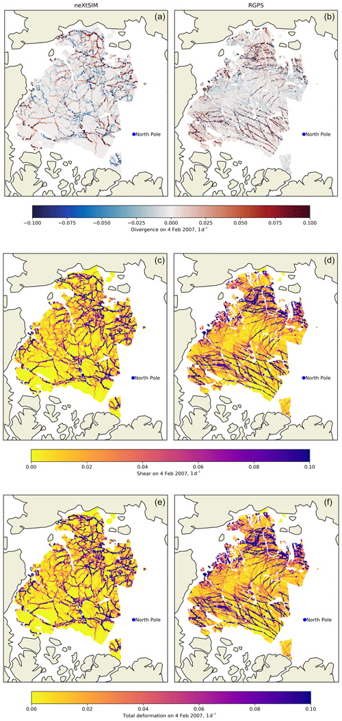
Figure 1 Divergence, shear and total sea ice deformation rates per day (top to bottom), as simulated by the model (a, c, e) and observed from satellite (b, d, f). The deformation rates are calculated over a timescale of 3 d. In order to get a better spatial coverage, we show all the deformation rates calculated within the period of 7 d, centered on 4 February 2007.

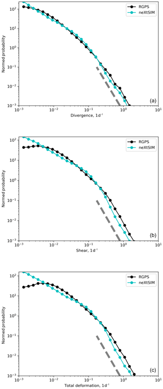
Figure 2 Probability density functions of the absolute divergence, shear and total deformation rates shown in the maps of Fig. 1 for the model (cyan) and the RGPS observations (black). The deformations are calculated over a timescale of 3 d and a spatial scale of 7.5 km (mean of the square root of the triangle's surface area, for which the deformations are calculated). Power-law fits of the tails of the distributions for the model and the RGPS observations and for each invariant give similar exponents ranging from −2.9 and −3.2. The dashed line is shown for reference and corresponds to a power law with an exponent equal to −3.

4.1 Spatial scaling analysis

Figure 3a shows the winter mean of the spatial scaling analysis for the observations and model calculated for a T=3 d temporal scale. We found that both model and observations statistics follow power laws. We used logarithmically spaced bins and applied an ordinary least-squares method to the binned data in log–log space to get a reasonably accurate estimate of the power-law fits (Stern et al., 2018). The deformation rates are very well captured by the model across scales. However, the first and second moments of the distributions are slightly overestimated by the model compared to the observations, whatever the spatial scale considered was. For example, at the nominal scale of 7.5 km, the first and second moments are overestimated by a factor of 2 compared to the observations. This may be due to one or several of the following factors: (1) inaccuracies in the atmospheric forcing, (2) our choice of mechanical parameters values (Weiss and Dansereau, 2017) or (3) the value of the atmospheric drag coefficient (e.g., Bouchat and Tremblay, 2017). It is especially important to note that the simulated deformation rate has not been tuned with respect to the MEB mechanical parameters in the present simulations. We consider such tuning to be out of the scope of this study, which focuses on the ability to reproduce the observed scaling (exponents of the power laws) and, in particular, their multi-fractal properties (nonlinearity of the structure function). The simulated and observed structure functions (i.e., the dependence of the scaling exponents on the moment order) β(q) are shown in Fig. 3b. The spatial scaling obtained for both the model and the RGPS are clearly multi-fractal, as their structure functions can be both approximated by a quadratic function as defined by Eq. (4) with coefficients a=0.11 and 0.13, respectively. These values, corresponding to the curvature of the structure functions, are very close to those reported in previous studies (a=0.13–0.14; Marsan et al., 2004; Rampal et al., 2016). It is important to note that the bars on this graph are estimated from the minimal and maximal local scaling exponent values, as in Bouillon and Rampal (2015a) and hence correspond to upper-bound estimates rather than to error bars. This good agreement is a relevant indication that the scaling in the simulated deformation fields is consistent with that observed between 7.5 and 580 km.

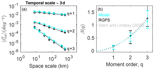
Figure 3 Spatial scaling analysis of the observed (black) and simulated (blue) total deformation rate calculated over a timescale of 3 d from the motion of the same triplets in the model and the RGPS dataset. (a) Moments $\langle {\dot{\mathit{\epsilon }}}_{\mathrm{tot}}^q\rangle$ of order $q=\mathrm{1},\mathrm{2}$ and 3 of the distributions of the total deformation rate ${\dot{\mathit{\epsilon }}}_{\mathrm{tot}}$ calculated at a temporal scale of 3 d and space scales varying from 7.5 to 580 km. The solid lines indicate the associated power-law scaling $\langle {\dot{\mathit{\epsilon }}}_{\mathrm{tot}}^q\rangle \sim L^{-\mathit{\beta }\left(q\right)}$. (b) Corresponding structure functions β(q) for both the model and observation, where β indicates the exponent of the power-law fits and q is the moment order. The bars indicate the deviation from the power law as they correspond to the minimum and maximum power-law exponents obtained for two successive spatial scales, as in Bouillon and Rampal (2015a), and can be viewed as an estimation of the goodness of the fit.

Using successive and contiguous snapshots throughout the winter, a time series of the value of the spatial scaling exponent β obtained for the mean deformation rates (q=1) is calculated and plotted on Fig. 4. It shows that the spatial scaling exponent varies between −0.1 and −0.34. These exponents are in good agreement with the 1-month running means of the scaling exponents calculated by Stern and Lindsay (2009) for the entire period covered by the RGPS dataset (1996–2008). The scaling exponent for the mean is about −0.2 on average over the whole winter period for the simulated and observed total deformation rates, which is also the value found by Marsan et al. (2004) for a snapshot of deformation rates calculated over a 3 d period centered on 6 November 1997. We also note that the model reproduces the observed variability of the scaling exponent throughout the whole period well.

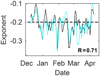
Figure 4 Time series of spatial scaling exponents for the mean total deformation (i.e., q=1) calculated for individual snapshots and at a temporal scale of T=3 d for the model (cyan) and the RGPS observations (black). The dashed line is shown only for reference and corresponds to the value of 0.2 reported in Marsan et al. (2004) for the 3 d deformation calculated over a period centered on 6 November 1997.

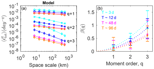
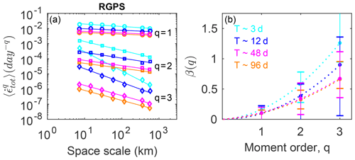
We further characterize the properties of the spatial scaling for both the model and observations by exploring its dependence on the temporal scale, T. We find that the estimated spatial scaling exponent, β, decreases with increasing T, although this behavior is only obvious for the moments of order 2 and 3 (Figs. 5a and 6a). This seems to correspond to the existence of space–time coupling of the scaling properties of sea ice deformation. This property was originally suggested by Rampal et al. (2008) from the result of their scaling analysis of buoy pair dispersion and was further explained in Marsan and Weiss (2010) as being a possible characteristic of brittle deformation at geophysical scales. To our knowledge, this is the first time such coupling is obtained from a sea ice model simulation run at such relatively coarse spatial resolution. The origin of this coupling has been previously proposed to be linked to the complex correlation patterns related to chain triggering of ice-quakes (Marsan and Weiss, 2010). Further study is, however, needed to explore this hypothesis, which is out of the scope of this paper.

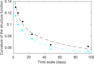
We also note a decrease in the multi-fractal character of the spatial scaling (i.e., the curvature of β(q)) when increasing the timescales from T=3 to T=96 d (Figs. 5b and 6b). For both the model and the observations, we observe that the multi-fractality property is present for all scales considered in this study, although a decrease in the degree of multi-fractality is observed as the scale increases. The curvature values decrease from 0.115 to 0.054 for the model and from 0.13 to 0.063 for the observations following a power law (Fig. 7). While the general behavior of decreasing the degree of multi-fractality of the spatial scaling as the timescale increases is captured by the model, we note that the degree of multi-fractality of the deformation is systematically underestimated by the model compared to the observations. This could either be attributed to an inaccurate position, a lack of extreme events in the atmospheric forcing, or an inadequate or insufficiently tuned parameterization of the damage healing in the model. In any case, the reason for this discrepancy should be further explored but is out of scope of the present paper.

Figure 5 Same as Fig. 3 but for the model at various temporal scales.

Figure 6 Same as Fig. 3 but for the RGPS observations at various temporal scales.

Figure 7 Curvature of the structure function as a function of the timescale T for the model (cyan dots) and the RGPS observations (black dots). The dashed lines are power-law fits (in the least-squares sense) through the data.

4.2 Temporal scaling analysis

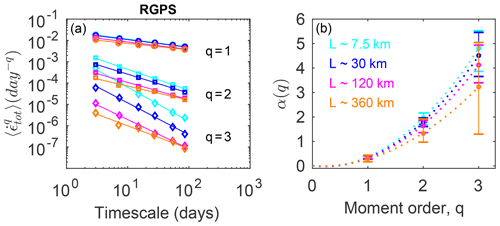
The results of the temporal scaling analysis for L=7.5 km is shown in Fig. 8a. We see a robust and very similar power-law scaling for the two first moments ($q=\mathrm{1},\mathrm{2}$) for both the model and observations between T=3 d (i.e., the temporal resolution of the observations) and T=96 d. In previous studies based on drifting buoy trajectories, whose positions are sampled at higher frequency, it has been suggested that the temporal scaling for the mean total deformation holds down to 1 h (Hutchings et al., 2011). A recent study based on very-high-resolution ship radar measurements has demonstrated that it holds down even to 10 min (Oikkonen et al., 2017). Here, we obtain a perfect agreement between the slope ($\sim -\mathrm{0.3}$) of the temporal scaling for the mean deformation rates estimated by Oikkonen et al. (2017) and those estimated from the RGPS data and the present model simulations.

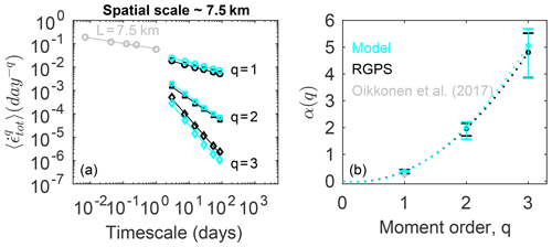
Figure 8 Temporal scaling analysis of the total deformation rate derived from the motion of the same triplets with initial surface area of 7.5 km for the model (cyan) and the RGPS observations (black). (a) Moments $\langle {\dot{\mathit{\epsilon }}}_{\mathrm{tot}}^q\rangle$ of order $q=\mathrm{1},\mathrm{2}$ and 3 of the distributions of the total deformation rate ${\dot{\mathit{\epsilon }}}_{\mathrm{tot}}$ calculated at a spatial scale of 7.5 km and timescales varying from 3 to 100 d. The solid lines indicate the associated power-law scaling $\langle {\dot{\mathit{\epsilon }}}_{\mathrm{tot}}^q\rangle \sim t^{-\mathit{\alpha }\left(q\right)}$. Grey dots correspond to the mean total deformation rates obtained by Oikkonen et al. (2017) at a same spatial scale of 7.5 km and for timescales ranging from 3 h to 1 d. (b) Corresponding structure functions α(q) for both the model and RGPS observations, where α indicates the exponent of the power-law fits and q is the moment order. The bars indicate the deviation from the power law as they correspond to the minimum and maximum power-law exponents obtained for two successive temporal scales and can be viewed as an estimation of the goodness of the fit.

We note, however, that the third moments of the distributions are slightly underestimated by the model at all timescales. This means that the proportion of extreme deformation events compared to lower ones is too small or that their values are too low in the simulation. This may come from the inaccuracy of the relatively coarse (30 km) atmospheric reanalysis we use to force our model and that is known to poorly resolve the most extreme low pressure systems, a common shortcoming of all the available global or regional atmosphere reanalysis to date. Another explanation could be the fact that we have not tuned the MEB rheology parameters to reproduce the proportion of extreme deformation events versus the less extreme events. In this rheology, the coupling between the damage and the mechanical behavior of sea ice is nonlinear and it is therefore expected that varying parameter values can change the proportion of the simulated extreme events, i.e., the skewness of the distribution of deformation rates.

As in the spatial domain, the temporal scaling is found to be multi-fractal for the model and observations, and the match is remarkably good. The curvature values (i.e., the coefficient c in Eq. 5) are 0.67 for the model and 0.62 for the observations. This suggests that the multi-fractal character of the temporal scaling is stronger than the spatial scaling and possibly a robust property of sea ice deformation, at least in the wintertime, independent of the observed change in sea ice cover state and the associated shift of its dynamical regime during the period 1996–2006 (e.g., Rampal et al., 2009a, b). We note that the values of curvature of the structure functions obtained here cannot be directly compared to the one reported in Weiss and Dansereau (2017) since in their paper the authors are plotting the normalized moments $\langle {\dot{\mathit{\epsilon }}}_{\mathrm{tot}}^q{\rangle }^{\mathrm{1}/q}$ of the distribution versus the temporal scale instead of the actual moments $\langle {\dot{\mathit{\epsilon }}}_{\mathrm{tot}}^q\rangle$ as we do here.

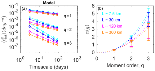
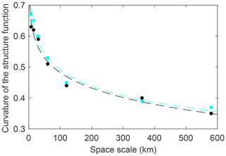
We also investigate the dependence of the temporal scaling on the spatial scale of observation, L, for both the model and RGPS data (Figs. 9a and 10a). We find that the scaling exponent, α, decreases with L. Similar to the spatial scaling analysis performed in Sect. 4.1, we find here the signature of a space-time coupling in the scaling properties of sea ice deformation. The multi-fractal character of the temporal scaling holds at all the spatial scales considered here (L=7.5 to L=580 km) and is similar in the model and observations (Figs. 9b and 10b). The curvature values are going from 0.67 down to 0.37 for the model and from 0.63 to 0.35 for the observations following a power law (Fig. 11). The decrease in the degree of multi-fractality of the temporal scaling as the space scale increases, as seen in the observations, is remarkably well captured by the model.

Figure 9 Same as Fig. 8 but for the model at various spatial scales.

Figure 10 Same as Fig. 8 but for the RGPS observations at various spatial scales.

Figure 11 Curvature of the structure function as a function of the space scale L for the model (cyan dots) and the RGPS (black dots). The dashed lines are power-law fits (in the least-squares sense) to the data.

5 Discussion

Our statistical analyses have shown that the neXtSIM model correctly reproduces the distribution of sea ice deformation rates, its scaling properties in both the space and time domains and its multi-fractal behavior. In particular, it is the first time that multi-fractality in the time domain is shown to be reproduced in a sea ice model.

The MEB rheology was developed with the aim of improving the representation of the physics of sea ice continuum models by including the ingredients hypothesized by Weiss and Dansereau (2017) to possibly play an important role in the emergence of multi-fractal heterogeneity and intermittency of sea ice deformation. This hypothesis is based on the analysis of observational data that have highlighted the existence of multi-fractality of sea ice deformation in space and time (Rampal et al., 2008; Bouillon and Rampal, 2015b; Weiss and Dansereau, 2017) and on a close and arguably sound analogy that can be made with other large-scale solids sharing these properties, such as the Earth's crust (Weiss et al., 2009). According to Weiss and Dansereau (2017) the ingredients are a threshold mechanism for brittle fracturing, some disorder that represents the natural heterogeneity of the material at the mesoscale, long-range elastic interactions within the ice cover that promote avalanches of fracturing events through a cascading mechanism, post-fracturing relaxation of elastic stresses through viscous-like relaxation and a slow restoring or healing mechanism of the sea ice mechanical properties. We argue that the results obtained here are at least a sound demonstration that a model including these ingredients can indeed reproduce complex aspects of sea ice deformation, such as its multifractality.

We show here that the spatial scaling of sea ice deformation simulated in a realistic setup by neXtSIM holds down to the nominal resolution of the mesh, a result that is in agreement with previous analyses of the MEB model in idealized simulations (Dansereau et al., 2016) and realistic ones (Rampal et al., 2016). It means that neXtSIM does not need to be run at higher spatial resolution in order to reproduce the observed scalings, as, e.g., Hutter et al. (2018) do when running at about 1 km resolution in order to resolve sea ice deformation at scale of about 10 km. Localizing the deformation at the nominal model resolution also means that related quantities, such as ridges, leads and linear kinematic features, are better resolved, although this is not investigated directly here. It is also important to note that using a Lagrangian scheme with adaptive remeshing instead of, for instance, a Eulerian finite volume scheme, helps in preserving such features once formed but plays no role in their formation.

We also show that this spatial localization and the multi-fractal character of the simulated mean sea ice deformation is resolution-independent in the model (see Fig. 12). However, despite the fact that the scaling remains multi-fractal when neXtSIM runs at coarser resolutions (e.g., 15 or 30 km), the level of multi-fractality is decreasing with decreasing resolution. Indeed, the second and third moments of deformation rates from the 15 and 30 km runs differ from the results obtained from the 7.5 km run (Fig. 12b), which suggests an underestimation of extreme deformation events at the smaller spatial scales with increasing model resolution. Nevertheless, the representation of multifractality at all resolutions implies that neXtSIM could be adequately used to explore a wider range of space scales and timescales than those covered by the currently available observations of the global Arctic. In particular, it could allow us to “zoom in” and explore the statistical properties of sea ice deformation at subsatellite observation scales, which are of increasing interest for both regional to global climate modeling and operational forecasting. A model that could otherwise not represent the multi-fractal character of sea ice deformation and would only reproduce a mono-fractal scaling would greatly underestimate extreme deformation events and their impact on sea ice conditions, e.g., the presence (or lack thereof) of leads and ridges, at such scales.

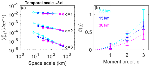
Figure 12 Spatial scaling analysis of the simulated deformation derived from the motion of triplets over a timescale of T=3 d in three different model runs at 7.5, 15 and 30 km resolution, respectively. (a) Moments $\langle {\dot{\mathit{\epsilon }}}_{\mathrm{tot}}^q\rangle$ of order $q=\mathrm{1},\mathrm{2}$ and 3 of the distributions of the total deformation rate ${\dot{\mathit{\epsilon }}}_{\mathrm{tot}}$ calculated at a temporal scale of 3 d and for spatial scales varying from 7.5 to 580 km. The solid lines indicate the associated power-law scaling $\langle {\dot{\mathit{\epsilon }}}_{\mathrm{tot}}^q\rangle \sim L^{-\mathit{\beta }\left(q\right)}$ as in Fig. 3. (b) Corresponding structure functions β(q) where β indicates the exponent of the power-law fits and q is the moment order. The bars indicate the deviation from the power law as they correspond to the minimum and maximum power-law exponents obtained for two successive spatial scales, as in Bouillon and Rampal (2015a), and thus correspond to upper-bound estimates and can be viewed as an estimation of the goodness of the fit.

A model that allows for reproducing sea ice deformation and its scaling properties down to its nominal resolution does not preclude the need for appropriate sub-grid-scale parameterizations. On the contrary, we believe that physically sound parameterizations are indeed required and that the knowledge of the distribution of deformation rates at the sub-grid scale made possible by neXtSIM could be highly valuable in terms of informing these parameterizations. An appropriate sub-grid-scale parametrization should link the deformation simulated at the scale of the grid cell with the scale at which deformation really occurs within the ice cover, which is the size of individual leads and ridges.

Moreover, we argue that, as sea ice deformation is strongly tied to other model variables, such as drift, lead fraction and thickness distribution, a proper simulation of these variables is a necessary prerequisite to using models for investigating various coupled ocean–ice–atmosphere processes, and their impact on their immediate vicinity and on the polar climate system. For example, the accuracy of neXtSIM in reproducing the observed statistical properties of sea ice deformation as demonstrated in this paper is thought to go hand-in-hand with its capability of representing the observed properties of lead fraction. This is the subject of a parallel study that is in preparation.

6 Conclusions

In this study we have compared the deformation rates simulated by neXtSIM to those derived from RGPS observations on the basis of their distributions and have shown how these distributions scale in time and space. The conclusions of our analysis are as follows.

• The neXtSIM model reproduces the first, second and third moments of the statistical distribution of observed sea ice deformation rates and how it scales in space and time well. In particular, this is the first time the observed scaling invariance in the temporal domain (i.e., intermittency) of sea ice deformation is shown to be reproduced by a model on a realistic pan-Arctic setup over such a large range of scales.

• Sea ice deformation rates calculated over a temporal scale of 3 d scale in space from the scale of the model (mesh resolution) and observations up to about 700 km in a multi-fractal manner.

• Sea ice deformation rates calculated over a spatial scale of 7.5 km scale in time over the range of 3 d to 3 months in a multi-fractal manner.

• A space–time coupling in the scaling properties of sea ice deformation is shown to be reproduced by the model. This suggests that neXtSIM could be the proper tool for studying the physical meaning and origin of this coupling, in the context of brittle deformation of geophysical solids.

• The simulated mean sea ice deformation rates and their associated scaling invariance characteristics are resolution-independent, i.e., when running the neXtSIM model at resolutions of 7.5, 15 or 30 km. The most extreme deformation events may be missed, however, if running at coarser resolutions, i.e., the second- and third-order moments may be underestimated compared to the high-resolution run.

• As the mono-fractal versus multi-fractal character of the scaling of deformation rates is the discriminating factor for the heterogeneity and intermittency of the deformation, we suggest that a multi-fractal scaling analysis could be considered a meaningful validation step before further analyzing sea ice model outputs that could be influenced by sea ice dynamics.

• The good agreement between the model and observations motivates the use of neXtSIM as a tool to further investigate physical processes that are highly sensitive to sea ice deformation.

Appendix A: Model description

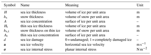
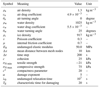
This section presents the dynamical and thermodynamical components of neXtSIM. The wave-in-ice module implemented by Williams et al. (2017) is not included here. Prognostic sea ice variables are listed in Table A1 and all parameter values are listed in Table A2.

Table A1 List of variables used in neXtSIM.

Table A2 Parameters used in the model with their values for the simulation at 7.5 km resolution used for this study.

A1 Dynamical core

The evolution equation for sea ice velocity comes from vertically integrating the horizontal sea ice momentum equation as follows:

$$\begin{array}{}\text{(A1)}& \begin{array}{rl}{\mathit{\rho }}_{i}H{\displaystyle \frac{D\mathit{u}}{Dt}}& =\mathrm{\nabla }\cdot \left(H\mathit{\sigma }\right)+{\mathit{\tau }}_{\mathrm{a}}+{\mathit{\tau }}_{\mathrm{w}}+{\mathit{\tau }}_{\mathrm{b}}-{\mathit{\rho }}_{\mathrm{i}}H\\ & \left(f\mathit{k}\times \mathit{u}+g\mathrm{\nabla }\mathit{\eta }\right).\end{array}\end{array}$$

The parameter ρ_i is the ice density; H is the mean ice thickness per unit grid cell area; σ is the sea ice internal stress tensor; and τ_a, τ_w, and τ_b are the surface wind, ocean, and basal stresses, respectively, as defined in Rampal et al. (2016). The parameter f is the Coriolis frequency, k is the upward pointing unit vector, g is the acceleration due to gravity and η is the ocean surface elevation. In the region with only thin ice or with thick ice thickness lower than a given threshold (defining our ice edge), the momentum equation is replaced by Laplace's equation so that the velocity linearly decreases from the ice edge to the nearest coast (see Samaké et al., 2017). The additional ice pressure term introduced in Rampal et al. (2016) is not included here.

Following Dansereau et al. (2016), the evolution equation for the internal stress takes the form of the Maxwell constitutive law:

$$\begin{array}{}\text{(A2)}& {\displaystyle \frac{D\mathit{\sigma }}{Dt}}+{\displaystyle \frac{\mathit{\sigma }}{\mathit{\lambda }}}=E\mathit{K}:\dot{\mathit{\epsilon }}\left(\mathit{u}\right),\end{array}$$

where λ is the relaxation time for the stress, E, is the elastic modulus and $\dot{\mathit{\epsilon }}$, the strain rate tensor, is defined as

$$\begin{array}{}\text{(A3)}& \dot{\mathit{\epsilon }}\left(\mathit{u}\right)={\displaystyle \frac{\mathrm{1}}{\mathrm{2}}}\left(\mathrm{\nabla }\mathit{u}+(\mathrm{\nabla }\mathit{u}{)}^T\right).\end{array}$$

Plane stress conditions are assumed and the stiffness tensor K reads

$$\begin{array}{}\text{(A4)}& \left[\begin{array}{l}{\left(\mathit{K}:\mathit{\epsilon }\right)}_{\mathrm{11}}\\ {\left(\mathit{K}:\mathit{\epsilon }\right)}_{\mathrm{22}}\\ {\left(\mathit{K}:\mathit{\epsilon }\right)}_{\mathrm{12}}\end{array}\right]={\displaystyle \frac{\mathrm{1}}{\mathrm{1}-{\mathit{\nu }}^{\mathrm{2}}}}\left(\begin{array}{lll}\mathrm{1}& \mathit{\nu }& \mathrm{0}\\ \mathit{\nu }& \mathrm{1}& \mathrm{0}\\ \mathrm{0}& \mathrm{0}& {\displaystyle \frac{\mathrm{1}-\mathit{\nu }}{\mathrm{2}}}\end{array}\right)\left[\begin{array}{l}{\mathit{\epsilon }}_{\mathrm{11}}\\ {\mathit{\epsilon }}_{\mathrm{22}}\\ \mathrm{2}{\mathit{\epsilon }}_{\mathrm{12}}\end{array}\right],\end{array}$$

where ν is Poisson's ratio.

As in Dansereau et al. (2016), both the elastic modulus, E, and the relaxation time are functions of the ice concentration, A, and the level of damage, d. The level of damage is a scalar, grid-scale variable that represents the density of fractures at the sub-grid scale. Its value is 0 for an undamaged and 1 for a “completely” damaged material, which we note is the opposite convention to that of Dansereau et al. (2016). The elastic modulus is a linear function of d:

$$\begin{array}{}\text{(A5)}& E(A,d)=E_{\mathrm{0}}(\mathrm{1}-d)f\left(A\right),\end{array}$$

where E₀ is the undamaged elastic modulus and f(A) introduces a dependence on the ice concentration via the following exponential function:

$$\begin{array}{}\text{(A6)}& f\left(A\right)={\mathrm{e}}^{-c^{\ast }(\mathrm{1}-A)},\end{array}$$

where c^∗ is the ice compactness parameter introduced by Hibler (1979). As in Dansereau et al. (2016), the relaxation time is a power function of d:

$$\begin{array}{}\text{(A7)}& \mathit{\lambda }\left(d\right)={\mathit{\lambda }}_{\mathrm{0}}(\mathrm{1}-d{)}^{\mathit{\alpha }-\mathrm{1}},\end{array}$$

where λ₀ is its undamaged value and α is a constant exponent greater than 1. Here, we use the values α=5 and λ₀=10⁷ s (115 d, as in the realistic Maxwell-EB simulations of Dansereau et al., 2017) to ensure that the relaxation of stresses is virtually zero over an undamaged ice cover but is significant when the ice is damaged.

The evolution of the damage is controlled by the location of the predicted stress state relative to the failure envelope, which is defined in terms of the principal stress components

$$\begin{array}{}\text{(A8)}& {\displaystyle }& {\displaystyle }{\mathit{\sigma }}_{\mathrm{1}}=-{\displaystyle \frac{{\mathit{\sigma }}_{\mathrm{11}}+{\mathit{\sigma }}_{\mathrm{22}}}{\mathrm{2}}}+\sqrt{{\left({\displaystyle \frac{{\mathit{\sigma }}_{\mathrm{11}}-{\mathit{\sigma }}_{\mathrm{22}}}{\mathrm{2}}}\right)}^{\mathrm{2}}+{\mathit{\sigma }}_{\mathrm{12}}^{\mathrm{2}}},\text{(A9)}& {\displaystyle }& {\displaystyle }{\mathit{\sigma }}_{\mathrm{2}}=-{\displaystyle \frac{{\mathit{\sigma }}_{\mathrm{11}}+{\mathit{\sigma }}_{\mathrm{22}}}{\mathrm{2}}}-\sqrt{{\left({\displaystyle \frac{{\mathit{\sigma }}_{\mathrm{11}}-{\mathit{\sigma }}_{\mathrm{22}}}{\mathrm{2}}}\right)}^{\mathrm{2}}+{\mathit{\sigma }}_{\mathrm{12}}^{\mathrm{2}}},\end{array}$$

with the convention that compressive stresses are positive.

Here, the envelope combines a Mohr–Coulomb failure criterion and maximum tensile and compressive stress criteria. These are given by

$$\begin{array}{}\text{(A10)}& {\displaystyle }{\mathit{\sigma }}_{\mathrm{1}}-q{\mathit{\sigma }}_{\mathrm{2}}& {\displaystyle }\le {\mathit{\sigma }}_c\text{(Mohr–Coulomb criterion)},\text{(A11)}& {\displaystyle }-{\displaystyle \frac{{\mathit{\sigma }}_{\mathrm{1}}+{\mathit{\sigma }}_{\mathrm{2}}}{\mathrm{2}}}& {\displaystyle }\le {\mathit{\sigma }}_{T\text{max}}\text{(tensile stress criterion)},\text{(A12)}& {\displaystyle \frac{{\mathit{\sigma }}_{\mathrm{1}}+{\mathit{\sigma }}_{\mathrm{2}}}{\mathrm{2}}}& {\displaystyle }\le {\mathit{\sigma }}_{N\text{max}}\text{(compressive stress criterion)},\end{array}$$

where $q={\left[{\left({\mathit{\mu }}^{\mathrm{2}}+\mathrm{1}\right)}^{\mathrm{1}/\mathrm{2}}+\mathit{\mu }\right]}^{\mathrm{2}}$, ${\mathit{\sigma }}_c=\frac{\mathrm{2}c}{\left[{\left({\mathit{\mu }}^{\mathrm{2}}+\mathrm{1}\right)}^{\mathrm{1}/\mathrm{2}}-\mathit{\mu }\right]}$, μ is the internal friction coefficient, c is the cohesion, σ_T max is the maximal tensile strength and σ_N max the maximum compressive strength (see Table A2). The cohesion, c, is scaled as a function of the model spatial resolution, as described in Bouillon and Rampal (2015a).

When one of the damage criteria is met, d is modified by multiplying (1−d) with Ψ, or

$$\begin{array}{}\text{(A13)}& d\leftarrow \mathrm{1}-\mathrm{\Psi }(\mathrm{1}-d),\end{array}$$

where

$$\begin{array}{}\text{(A14)}& \mathrm{\Psi }=\left\{\begin{array}{ll}\frac{{\mathit{\sigma }}_c}{{\mathit{\sigma }}_{\mathrm{1}}-q{\mathit{\sigma }}_{\mathrm{2}}}& \text{ if }{\mathit{\sigma }}_{\mathrm{1}}-q{\mathit{\sigma }}_{\mathrm{2}}>{\mathit{\sigma }}_c\\ \frac{\mathrm{2}{\mathit{\sigma }}_{T\text{max}}}{-{\mathit{\sigma }}_{\mathrm{1}}+{\mathit{\sigma }}_{\mathrm{2}}}& \text{ if }-\frac{{\mathit{\sigma }}_{\mathrm{1}}+{\mathit{\sigma }}_{\mathrm{2}}}{\mathrm{2}}>{\mathit{\sigma }}_{T\text{max}}\\ \frac{\mathrm{2}{\mathit{\sigma }}_{N\text{max}}}{{\mathit{\sigma }}_{\mathrm{1}}+{\mathit{\sigma }}_{\mathrm{2}}}& \text{ if }\frac{{\mathit{\sigma }}_{\mathrm{1}}+{\mathit{\sigma }}_{\mathrm{2}}}{\mathrm{2}}>{\mathit{\sigma }}_{N\text{max}}\end{array}\right..\end{array}$$

Healing is included here to represent the counteracting effect of refreezing of water within leads on the level of damage of the ice cover. It is implemented via a constant term in the damage evolution equation:

$$\begin{array}{}\text{(A15)}& {\displaystyle \frac{Dd}{Dt}}={\displaystyle \frac{(\mathrm{1}-d)(\mathrm{1}-\mathrm{\Psi })}{T_{\mathrm{d}}}}-{\displaystyle \frac{\mathrm{1}}{T_{\mathrm{h}}}},\end{array}$$

where T_h is the characteristic time for healing and T_d is the characteristic time for damaging (Dansereau et al., 2016).

A2 Ice thickness redistribution and thermodynamics

neXtSIM includes a multi-category model inspired from Stern and Rothrock (1995), i.e., considering three categories: thick ice, thin ice and open water. In our implementation the thin ice is only newly formed ice, so ice will only be transferred from the thin ice category to thick ice but not in the reverse direction. In addition, we do not apply additional open-water source terms or use the formulation of Gray and Morland (1994) to keep the ice concentration less than 1. (We simply redistribute ice and snow volume if this occurs.) Thin ice is described by its concentration, A_t, volume per unit area, H_t, and snow volume per unit area, h_s,t. Thick ice is described by the concentration, A, volume per unit area, H, and snow volume per unit area, h_s. We assume that the thin ice has no mechanical strength and simply follows the motion of the surrounding thick ice.

Note that the total ice concentration and volume per unit area are A+A_t and H+H_t and the total snow volume per unit area is $h_{\mathrm{s}}+h_{\mathrm{s},\mathrm{t}}$.

Thin ice thickness is considered to be uniformly distributed with thickness $h_{\mathrm{t}}=H_{\mathrm{t}}/A_{\mathrm{t}}$ required to be between h_min=5 cm and h_max=27.5 cm. The evolution equations for A, H, h_s, A_t, H_t and h_s,t have the following form:

$$\begin{array}{}\text{(A16)}& {\displaystyle \frac{D\mathit{\varphi }}{Dt}}=-\mathit{\varphi }\mathrm{\nabla }\cdot \mathit{u}+{\mathrm{\Psi }}_{\mathit{\varphi }}+S_{\mathit{\varphi }},\end{array}$$

where ${\displaystyle \frac{D\mathit{\varphi }}{Dt}}$ is the material derivative that is defined for any scalar as

$$\begin{array}{}\text{(A17)}& {\displaystyle \frac{D\mathit{\varphi }}{Dt}}={\displaystyle \frac{\partial \mathit{\varphi }}{\partial t}}+(\mathit{u}\cdot \mathrm{\nabla })\mathit{\varphi }.\end{array}$$

Here ∇⋅u is the divergence of the horizontal velocity, Ψ_ϕ is a sink or source term due to ridging, and S_ϕ is a thermodynamical sink or source term. Volume conservation is imposed by setting ${\mathrm{\Psi }}_H=-{\mathrm{\Psi }}_{H_{\mathrm{t}}}$ and ${\mathrm{\Psi }}_{h_{\mathrm{s}}}=-{\mathrm{\Psi }}_{h_{\mathrm{s},\mathrm{t}}}$ and an additional constraint is that $A_{\mathrm{t}}+A\le \mathrm{1}$.

The evolution of A, H, A_t and H_t is computed following three main steps (variables updated in each step are denoted with a prime):

1. Advection. The scheme solves the equation:

   $$\begin{array}{}\text{(A18)}& {\displaystyle \frac{D\mathit{\varphi }}{Dt}}=-\mathit{\varphi }\mathrm{\nabla }\cdot \mathit{u},\end{array}$$

   for each conserved scalar quantity (A, H, A_t, H_t, etc.). For this paper, we use the purely Lagrangian scheme presented in Rampal et al. (2016). After this step the concentration could be larger than 1.

2. Mechanical redistribution. The scheme imposes the limit $A_{\mathrm{t}}+A\le \mathrm{1}$ on the total ice area by following the steps below.

   1. Compute the new open-water concentration as follows:

      $$\begin{array}{}\text{(A19)}& A_{\mathrm{0}}=max(\mathrm{0},\mathrm{1}-A-A_{\mathrm{t}}),\end{array}$$

      a source term for the open water could be added here (as in Stern and Rothrock, 1995) to represent sub-grid-scale convergence and divergence.

   2. Compute the new thin ice concentration as follows:

      $$\begin{array}{}\text{(A20)}& A_{{\mathrm{t}}^{\prime }}=max(\mathrm{0},min(\mathrm{1},\mathrm{1}-A-A_{\mathrm{0}}\left)\right).\end{array}$$

   3. Compute the transfer of thin ice if $A_{{\mathrm{t}}^{\prime }}<A_{\mathrm{t}}$ by setting the following equations:

      $$\begin{array}{}\text{(A21)}& {\displaystyle }{H}_{{\mathrm{t}}^{\prime }}& {\displaystyle }=H_{\mathrm{t}}{\displaystyle \frac{A_{{\mathrm{t}}^{\prime }}}{A_{\mathrm{t}}}},\text{(A22)}& {\displaystyle }{h}_{\mathrm{s},\mathrm{t}}^{\prime }& {\displaystyle }=h_{\mathrm{s},\mathrm{t}}{\displaystyle \frac{A_{{\mathrm{t}}^{\prime }}}{A_{\mathrm{t}}}},\text{(A23)}& {\displaystyle }{H}^{\prime }& {\displaystyle }=H+(H_{\mathrm{t}}-H_{{\mathrm{t}}^{\prime }}),\text{(A24)}& {\displaystyle }{h}_{{\mathrm{s}}^{\prime }}& {\displaystyle }=h_{\mathrm{s}}+(h_{\mathrm{s},\mathrm{t}}-h_{\mathrm{s},{\mathrm{t}}^{\prime }}),\text{(A25)}& {\displaystyle }\mathrm{\Delta }A& {\displaystyle }={\displaystyle \frac{A_{\mathrm{t}}-A_{{\mathrm{t}}^{\prime }}}{\mathit{\zeta }}}.\end{array}$$

      Here, we have transferred ice and snow volume from thin to thick ice in a conservative manner, but we will not try to conserve ice area; ζ is an aspect ratio parameter (tuned to 10), which causes ridging to preferentially increase ice thickness over ice area.

   4. Compute the new thick ice concentration as follows:

      $$\begin{array}{}\text{(A26)}& A^{\prime }=max(\mathrm{0},min(\mathrm{1},\mathrm{1}-A_{{\mathrm{t}}^{\prime }}-A_{\mathrm{0}}+\mathrm{\Delta }A\left)\right).\end{array}$$

   5. Apply more ridging if $(A^{\prime }+A_{{\mathrm{t}}^{\prime }})>\mathrm{1}$ by setting $A^{\prime }=\mathrm{1}-A_{{\mathrm{t}}^{\prime }}$.

3. Growth and melt. The source and sink terms from the thermodynamics are computed by applying the zero-layer Semtner (1976) vertical thermodynamics to the new ice category and that of Winton (2000) for the thick ice, as if the thickness was uniform and equal to H∕A for the thick ice and H_t∕A_t for the thin ice. Freezing of open water is computed as in Rampal et al. (2016) such that heat loss from the ocean that would cause super cooling is redirected to ice formation. The newly formed ice is transferred to the thin ice category and is assumed to have a thickness equal to h_min. The transfer from the thin ice to the thick ice and the lateral melting of thin ice are computed by applying the bounding limit h_max – if h_t>h_max, then we update the variables as follows:

   $$\begin{array}{}\text{(A27)}& {\displaystyle }{h}_{{\mathrm{t}}^{\prime }}& {\displaystyle }=h_{\max },\text{(A28)}& {\displaystyle }{A}_{{\mathrm{t}}^{\prime }}& {\displaystyle }={\displaystyle \frac{h_{\max }-h_{\min }}{h_{\mathrm{t}}-h_{\min }}}{A}_{\mathrm{t}},\text{(A29)}& {\displaystyle }{H}_{{\mathrm{t}}^{\prime }}& {\displaystyle }=A_{{\mathrm{t}}^{\prime }}*h_{{\mathrm{t}}^{\prime }},\text{(A30)}& {\displaystyle }{h}_{\mathrm{s},\mathrm{t}}^{\prime }& {\displaystyle }={\displaystyle \frac{A_{{\mathrm{t}}^{\prime }}}{A_{\mathrm{t}}}}{h}_{\mathrm{s},\mathrm{t}},\text{(A31)}& {\displaystyle }{H}^{\prime }& {\displaystyle }=H-(H_{{\mathrm{t}}^{\prime }}-H_{\mathrm{t}}),\text{(A32)}& {\displaystyle }{A}^{\prime }& {\displaystyle }=A-(A_{{\mathrm{t}}^{\prime }}-A_{\mathrm{t}}),\text{(A33)}& {\displaystyle }{h}_{{\mathrm{s}}^{\prime }}& {\displaystyle }=h_{\mathrm{s}}-(h_{\mathrm{s},\mathrm{t}}^{\prime }-h_{\mathrm{s},\mathrm{t}}).\end{array}$$

   The form of the reduction in thin ice concentration in (Eq. A28) is a little arbitrary, but we wanted to allow the possibility of the thin ice completely changing into thick ice at some point.