Eemian Greenland ice sheet simulated with a higher-order model shows strong sensitivity to surface mass balance forcing

The Greenland ice sheet contributes increasingly to global sea level rise. Its history during past warm intervals is a valuable reference for future sea level projections. We present ice sheet simulations for the Eemian interglacial period (∼130 000 to 115 000 years ago), a period with warmer-than-present summer climate over Greenland. The evolution of the Eemian Greenland ice sheet is simulated with a 3-D higher-order ice sheet model, forced with a surface mass balance derived from regional climate simulations. Sensitivity experiments with various surface mass balances, basal friction, and ice flow approximations are discussed. The surface mass balance forcing is identified as the controlling factor setting the minimum in Eemian ice volume, emphasizing the importance of a reliable surface mass balance model. Furthermore, the results indicate that the surface mass balance forcing is more important than the representation of ice flow for simulating the large-scale ice sheet evolution. This implies that modeling of the future contribution of the Greenland ice sheet to sea level rise highly depends on an accurate surface mass balance.

1 Introduction

The simulation of the Greenland ice sheet (GrIS) under past warmer climates is a valuable way to test methods used for sea level rise projections. This study investigates ice sheet simulations for the Eemian interglacial period. The Eemian (∼130 000 to 115 000 years ago; hereafter 130 to 115 ka) is the most recent warmer-than-present period in Earth's history and thereby provides an analogue for future warmer climates (e.g., Clark and Huybers, 2009; Yin and Berger, 2015). The Eemian summer temperature is estimated to have been 4–5 ^∘C above present over most Arctic land areas (e.g., Capron et al., 2017) and an ice core record from NEEM (the North Greenland Eemian Ice Drilling project in northwest Greenland; NEEM community members, 2013) indicates a local warming of 8.5±2.5 ^∘C (Landais et al., 2016) compared to pre-industrial levels. In spite of this strong warming, total gas content measurements from the Greenland ice cores at the Greenland Ice Sheet Project 2 (GISP2), Greenland Ice Core Project (GRIP), North Greenland Ice Core Project (NGRIP), and NEEM indicate an Eemian surface elevation no more than a few hundred meters lower than present (at these locations). NEEM data indicate that the ice thickness in northwest Greenland decreased by 400±250 m between 128 and 122 ka with a surface elevation of 130±300 m lower than the present at 122 ka, resulting in a modest sea level rise estimate of 2 m (NEEM community members, 2013). Nevertheless, coral-reef-derived global mean sea level estimates show values of at least 4 m above the present level (Overpeck et al., 2006; Kopp et al., 2013; Dutton et al., 2015). While this could indicate a reduced Antarctic ice sheet, the contribution from the GrIS to the Eemian sea level highstand remains unclear. Previous modeling studies focusing on Greenland (e.g., Letréguilly et al., 1991; Otto-Bliesner et al., 2006; Robinson et al., 2011; Born and Nisancioglu, 2012; Stone et al., 2013; Helsen et al., 2013) used very different setups and forcing, and show highly variable results.

Ice sheets lose mass either due to a reduced surface mass balance (SMB) or accelerated ice dynamical processes. Ice dynamical processes may have contributed to the Eemian ice loss, for example, through changes in basal conditions, similar to what is seen today and what is discussed for the future of the ice sheet. Zwally et al. (2002) associate surface melt with an acceleration of GrIS flow and argue that surface-melt-induced enhanced basal sliding provides a mechanism for rapid, large-scale, dynamic responses of ice sheets to climate warming. Several other studies have attributed the recent and future projected sea level rise from Greenland partly to dynamical responses. Price et al. (2011), for example, use a 3-D higher-order model to simulate sea level rise caused by the dynamical response of the GrIS, and they find an upper bound of 45 mm by 2100 (without assuming any changes to basal sliding in the future). This dynamical contribution is of similar magnitude to previously published SMB-induced sea level rise estimates by 2100 (40–50 mm; Fettweis et al., 2008). Pfeffer et al. (2008) provide a sea level rise estimate of 165 mm from the GrIS by 2100 based on a kinematic scenario with doubling ice transport through topographically constrained outlet glaciers. Furthermore, Robel and Tziperman (2016) present synthetic ice sheet simulations and argue that the early part of the deglaciation of large ice sheets is strongly influenced by an acceleration of ice streams as a response to changes in climate forcing.

In this study, we apply a computationally efficient 3-D higher-order ice flow approximation (also known as Blatter–Pattyn; BP; Blatter, 1995; Pattyn, 2003) implemented in the Ice Sheet System Model (ISSM; Larour et al., 2012; Cuzzone et al., 2018). Including higher-order stress gradients provides a comprehensive ice flow representation to test the importance of ice dynamics for modeling the Eemian GrIS. Furthermore, we avoid shortcomings in regions where simpler ice flow approximations, often used in paleo applications, are inappropriate, especially regions with fast-flowing ice in the case of the shallow ice approximation (SIA; Hutter, 1983; Greve and Blatter, 2009) and regions dominated by ice creep in the case of the shallow shelf approximation (SSA; MacAyeal, 1989; Greve and Blatter, 2009). The higher-order approximation is equally well suited to simulate slow- as well as fast-flowing ice.

Plach et al. (2018) show that the derivation of the Eemian SMB strongly depends on the SMB model choice. Here, we test SMB forcing derived from dynamically downscaled Eemian climate simulations and two SMB models (a full surface energy balance model and an intermediate complexity SMB model) as described in Plach et al. (2018). Furthermore, we perform sensitivity experiments varying basal friction for the entire GrIS, and localized changes below the outlet glaciers.

The aim of this study is to compare the impact of SMB and basal sliding on the evolution of the Eemian GrIS. Furthermore, employing a 3-D higher-order ice flow model, instead of simpler ice dynamical approximations often used in millennial-scale ice sheet simulations, is a novelty of this study. It allows us to evaluate the importance of the ice flow approximation used for Eemian studies.

2 Models and experimental setup

2.1 SMB methods

The SMB forcing is based on Eemian time slice simulations with a fast version of the Norwegian Earth System Model (NorESM1-F; Guo et al., 2019) representing the climate of 130, 125, 120, and 115 ka using respective greenhouse gas concentrations and orbital parameters (details in Plach et al., 2018). In the climate model simulations, the present-day GrIS topography is used. These global simulations are dynamically downscaled over Greenland with the regional climate model Modèle Atmosphérique Régional (MAR; Gallée and Schayes, 1994; de Ridder and Gallée, 1998; Gallée et al., 2001; Fettweis et al., 2006). Subsequently, the SMB is calculated with (1) a full surface energy balance (SEB) model as implemented within MAR (MAR-SEB) and (2) an intermediate complexity SMB model (MAR-BESSI; BErgen Snow SImulator; BESSI; Born et al., 2019). Both models are physically based SMB models including a snowpack explicitly solving for the impact of solar shortwave radiation (this is essential for the Eemian period which has a significantly different solar insolation compared to today, e.g., van de Berg et al., 2011; Robinson and Goelzer, 2014). MAR-SEB is bidirectionally coupled to the atmosphere of MAR (i.e., evolving SEB impacts atmospheric processes; for example, albedo changes impact surface temperature, cloud cover, and humidity), while MAR-BESSI is uncoupled. These two models are selected as the most plausible Eemian SMBs from a wider range of simulations discussed in Plach et al. (2018); they show a negative total SMB during the Eemian peak warming. While MAR-SEB is chosen as the control because it has been extensively validated against observations in previous studies (Fettweis, 2007; Fettweis et al., 2013, 2017), MAR-BESSI is used to test the sensitivity of the ice sheet simulations to the SMB forcing. MAR-SEB and MAR-BESSI employ a different temporal model time step; while MAR-SEB uses steps of 180 s, MAR-BESSI calculates in daily time steps. The longer time steps used by MAR-BESSI imply that extreme temperatures (e.g., lowest temperatures at night can lead to more refreezing) are damped and this is likely the cause for a lower amount of refreezing in MAR-BESSI compared to MAR-SEB. Furthermore, MAR-BESSI uses a simpler albedo representation than MAR-SEB. Lower refreezing and simpler steps in albedo changing from fresh snow to glacier ice are identified as the main reasons for more negative SMB, as calculated by MAR-BESSI. For a detailed discussion of the differences between the models, the reader is referred to Plach et al. (2018). The two different SMB models are employed to test the sensitivity of the ice sheet simulations to the prescribed SMB forcing.

All SMB time slice simulations are calculated offline using the modern ice surface elevation, given the lack of data constraining the configuration of the Eemian GrIS surface elevation. The evolution of the SMB with the changing ice surface elevation is simulated with local SMB–altitude gradients following Helsen et al. (2012, 2013). The SMB gradient method is used to calculate SMB–altitude gradients at each grid point from the surrounding grid points within a default radius of 150 km (linear regression of SMB vs. altitude). Since the SMB–altitude gradients in the accumulation and the ablation zones are very different, they are calculated separately. If the algorithm is unable to find more than 100 grid points (of either accumulation or ablation), the radius is extended until a threshold of 100 data points for the regression is reached. For simplicity, the local gradients are calculated from the respective pre-industrial SMB simulations. Further details on the SMB gradient method are discussed in Helsen et al. (2012).

Between the SMBs calculated for 130, 125, 120, and 115 ka, a linear interpolation is applied, giving a transient SMB forcing over 15 000 years. A more complicated interpolation approach is unnecessary given the smooth climate forcing and the uncertainties related to the Eemian climate and SMB simulations. Plach et al. (2018) give a detailed discussion of the simulated climate evolution and show, for example, an Eemian peak warming of 4–5 ^∘C over Greenland, which is in agreement with proxy reconstructions (NEEM community members, 2013; Landais et al., 2016). The SMBs in the present study (after being corrected for topography) are shown and discussed in Sect. 3.

2.2 The Ice Sheet System Model (ISSM)

The ISSM is a finite-element, thermo-mechanical ice flow model based on the conservation laws of momentum, mass, and energy (Larour et al., 2012) – here, model version 4.13 is used (Cuzzone et al., 2018). ISSM employs an anisotropic mesh, which is typically refined by using observed surface ice velocities, allowing fast-flowing ice (i.e., outlet glaciers) to be modeled at higher resolution than slow-flowing ice (i.e., interior of an ice sheet). Furthermore, ISSM offers inversion methods to ensure that an initialized model matches the observed (modern) ice sheet configuration (i.e., observed ice surface velocities are inverted for basal friction or ice rheology; Morlighem et al., 2010; Larour et al., 2012). While ISSM offers a large range of ice flow representations, in this study, the computationally efficient 3-D higher-order configuration (Cuzzone et al., 2018) is used. This configuration uses an interpolation based on higher-order polynomials between the vertical layers instead of the default linear interpolation which requires a much higher number of vertical layers to capture the sharp temperature gradient at the base of an ice sheet. By using a quadratic interpolation, five vertical layers are sufficient to capture the thermal structure accurately, while a linear vertical interpolation requires 25 layers to achieve a similar result. This lower number of vertical layers reduces the computational demand for the thermal model and the stress balance calculations, and makes it possible to run 3-D higher-order simulations for thousands of years. The simulations over 12 000 years in this study take between 3 and 4 weeks on a single node with 16 cores.

2.3 Experimental setup

All simulations (forced with MAR-SEB and MAR-BESSI) run from 127 to 115 ka following the Paleoclimate Modeling Intercomparison Project (PMIP4; Otto-Bliesner et al., 2017) experimental design and initiating the Eemian simulations at 127 ka with a modern GrIS. The thermal structure is derived using a thermal steady-state simulation with prescribed pre-industrial temperature at the ice surface (from the regional climate model simulations) and an enthalpy formulation (Aschwanden et al., 2012) at the base to determine the basal conditions (cold or temperate ice). At the base of the ice sheet, a prescribed geothermal heat flux (Shapiro and Ritzwoller, 2004) as provided by the SeaRISE dataset (Bindschadler et al., 2013) is imposed. The basal friction coefficients are kept constant over time and are derived from an inversion of spatially varying, observed surface velocities. In this case, an algorithm chooses the basal friction coefficients in a way that the modeled velocities match the observed velocities. In a first inversion, an initial ice viscosity is prescribed. After the thermal steady-state simulation, the ice viscosity is updated as a function of the new thermal profile (Cuffey and Paterson, 2010). In a second inversion, the basal friction coefficients are iterated to minimize three cost functions (Table 1). A map of the basal friction coefficients is provided as the Supplement to this paper. The inversion depends on the chosen ice flow approximation due to the different representations of the stress balance. Hence, simulations with the 2-D SSA and the 3-D higher-order approximation, respectively, use different inversions.

(Blatter, 1995; Pattyn, 2003)Paterson (1994, p. 151)Cuffey and Paterson (2010, p. 75)

Table 1 ISSM model parameters.

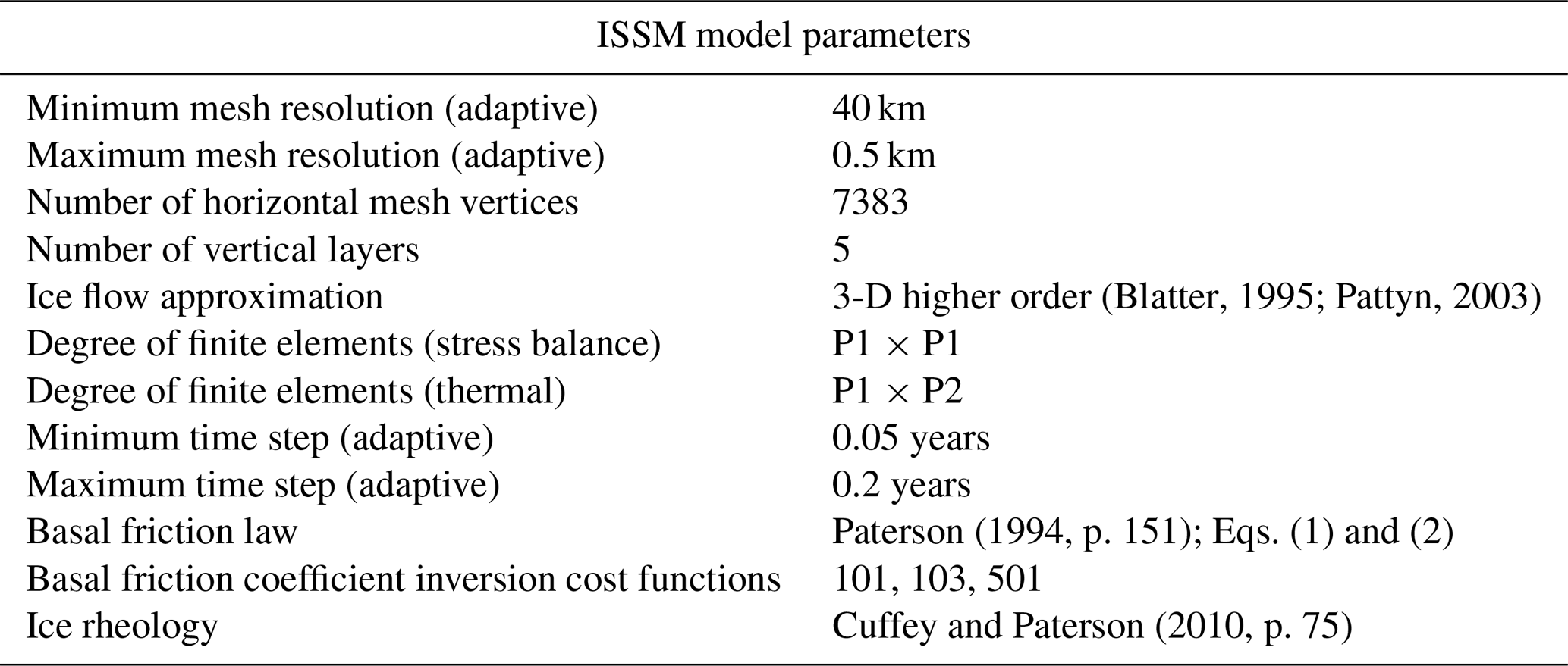
Degree of finite elements: P1 – linear finite elements, P2 – quadratic finite elements, horizontal × vertical; inversion cost functions: 101 – absolute misfit of surface velocities, 103 – logarithmic misfit of surface velocities, 501 – absolute gradient of the basal drag coefficients.

We use the ISSM default friction law (Larour et al., 2012; Schlegel et al., 2013) based on the empirically derived friction law by Paterson (1994, p. 151):

$$\begin{array}{}\text{(1)}& {\mathit{\tau }}_{\mathrm{b}}=-{\mathit{\alpha }}^{\mathrm{2}}{N}_{\mathrm{eff}}{\mathit{v}}_{\mathrm{b}},\end{array}$$

where τ_b is the basal shear stress (vector), α the basal friction coefficient (derived by inversion from surface velocities), N_eff the effective pressure of the water at the glacier base (i.e., the difference between the overburden ice stress and the water pressure), and v_b the horizontal basal velocity (vector). The effective pressure is simulated with a first-order approximation (Paterson, 1994):

$$\begin{array}{}\text{(2)}& N_{\mathrm{eff}}=g{\mathit{\rho }}_{\mathrm{ice}}H+{\mathit{\rho }}_{\mathrm{water}}{z}_{\mathrm{b}},\end{array}$$

where ρ_ice and ρ_water are the densities of ice and water, respectively, H is the ice thickness, and z_b is the bedrock elevation. From these equations, it follows that the initial (modern) basal friction coefficients stay constant, while the basal shear stress evolves over time with the ice thickness and the effective pressure.

Basal sensitivity experiments with changed basal friction are performed to investigate the importance of uncertainties related to basal friction. In order to minimize the number of 3-D higher-order experiments, a number of test experiments are performed with the simpler 2-D SSA configuration of ISSM to identify the range of basal friction coefficients which yield plausible results. For example, if the basal friction coefficients for the entire ice sheet are reduced by factors of 0.8 and 0.5 (in the 2-D SSA test experiments; not shown), the ice surface elevation at the NEEM location shows a late Eemian lowering of 300 and 800 m, respectively. Proxy data indicate a surface lowering of no more than 300 m (NEEM community members, 2013) at this point in time. In order to stay clearly within the proxy reconstructions, the friction for the entire ice sheet is reduced by a factor of 0.9 in the 3-D higher-order ice flow experiments. Two 2-D SSA experiments (forced with MAR-SEB and MAR-BESSI) are discussed in detail here to illustrate the difference of the two ice flow approximations (Table 2). A full list of 2-D SSA experiments is given as the Supplement to this paper.

Table 2 Overview of the experiments.

Due to the high computational demand of the 3-D higher-order model, compromises are necessary. The simulations are initiated with the modern GrIS topography and the bedrock remains fixed at modern values (glacial isostatic adjustment – GIA – is not yet implemented for transient simulations with ISSM). The ice sheet is initialized with observed ice surface velocities from Rignot and Mouginot (v4Aug2014; 2012). The anisotropic ice sheet mesh is refined with these velocities with a minimum resolution of 40 km in the slow interior and a maximum resolution of 0.5 km at the fast outlet glaciers. Since the mesh is based on observed velocities, the resolution of the mesh remains unchanged over time, and the ice sheet domain is fixed to the present-day ice sheet extent. The ice sheet can freely evolve within this domain but is unable to grow outside the present-day limits.

The air temperature prescribed at the ice surface remains fixed at pre-industrial levels. Ice formed during the 12 000-year simulations will only reach several hundred meters deep (not reaching the bottom layers which experience most deformation) and surface air temperature is not influencing the SMB (as it would in a degree-day model; Reeh, 1989) because SMB is computed by either MAR-SEB or MAR-BESSI, models that account for temperature changes over the Eemian (as simulated by NorESM).

The simplified transient ISSM model configuration does not explicitly resolve processes related to basal hydrology, ocean forcing, and calving. The ice rheology is calculated as a function of temperature following Cuffey and Paterson (2010, p. 75). Initial (modern) ice sheet surface, ice thickness, and bed topography are derived from BedMachine v3 (v2017-09-20; Morlighem et al., 2017). The most important parameters of the ice sheet model are summarized in Table 1. Finally, the shortcomings of this simplified configuration are discussed in Sect. 4.

2.4 Control and sensitivity experiments

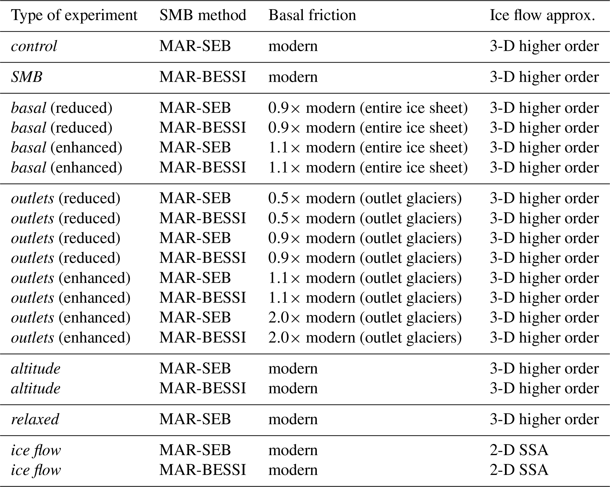
The experiments performed are described below and summarized in Table 2. As discussed in Sect. 2.1–2.3, the experiments test the sensitivity to two different SMB models as well as different representations of the basal friction: the control experiment applies SMB from MAR-SEB and unchanged (modern) basal friction; the SMB experiment tests the simplified but efficient SMB model, MAR-BESSI; the basal experiments test spatially uniform changes to the basal friction for the entire ice sheet; the outlets experiments test the sensitivity to changes of basal friction locally at the outlet glaciers (slowdown/speed-up of outlet glaciers, defined as high velocity regions with >500 m yr⁻¹). For the basal and outlets experiments, the basal friction coefficient is multiplied by factors of 0.9 and 1.1. Furthermore, the outlets experiments are repeated with more extreme factors of 0.5 and 2.0.

In additional experiments, with the more efficient SSA version of the model, a larger range of basal friction for the entire ice sheet is explored (doubling/halving of basal friction similar to Helsen et al., 2013). However, applying factors of 0.5 and 2.0 for the entire ice sheet results in unrealistic surface height changes at the central Greenland ice core locations (not shown). Therefore, these extreme changes of basal friction are only applied to the outlet glaciers in our 3-D higher-order experiments.

The altitude experiments test the impact of the SMB–altitude feedback by ignoring this feedback; which means that the transient SMB forcing is prescribed without correcting for altitude changes. Finally, we perform a relaxed experiment testing the sensitivity to a larger, relaxed initial ice sheet (with the same SMB and ice dynamics as the control experiment). This relaxed experiment starts with a larger ice sheet which is spun up for 10 000 years under constant pre-industrial SMB from MAR-SEB. The differences arising from the different ice flow approximations are illustrated in the ice flow experiments.

3 Results

The importance of the SMB forcing is illustrated in Fig. 1, showing the evolution of the Greenland ice volume in the control experiment (MAR-SEB; bold orange line) and the SMB sensitivity experiment (MAR-BESSI; bold purple line). The corresponding subsets of experiments testing the basal friction (basal, outlets) are indicated in lighter colors. There is a distinct difference between the model experiments forced with the two SMBs: forcing the ice sheet with MAR-SEB SMB (bold orange line) gives a minimum ice volume of 2.73×10¹⁵ m³ at 124.7 ka, corresponding to a sea level rise of 0.5 m – the basal sensitivity experiments give a range of 0.3 to 0.7 m (thin orange lines). On the other hand, the experiments forced with MAR-BESSI (bold purple line) give a minimum of 1.77×10¹⁵ m³ at 123.8 ka (2.9 m sea level rise) with a range from 2.7 to 3.1 m (thin purple lines). The minimum ice volume and the corresponding sea level rise from all experiments are summarized in Table 3.

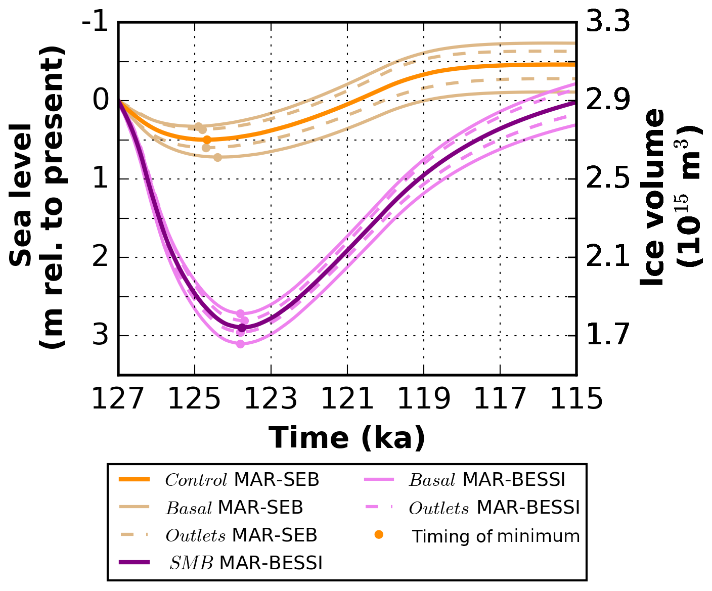
Figure 1 Evolution of the ice volume for the control (MAR-SEB, orange, bold) and the SMB (MAR-BESSI, purple, bold) experiments in comparison with the basal/outlets sensitivity experiments. The basal (friction $\times \mathrm{0.9}/\times \mathrm{1.1}$ for the entire ice sheet) and outlets sensitivity experiments (friction $\times \mathrm{0.5}/\times \mathrm{2.0}$ at the outlet glaciers) are indicated with thin solid and thin dashed lines, respectively. Note that the lower friction experiments give lower volumes. The minimum of the respective experiments is indicated with circles. See Table 3 for the exact values.

Table 3 Summary of the simulated ice sheet minima for all experiments.

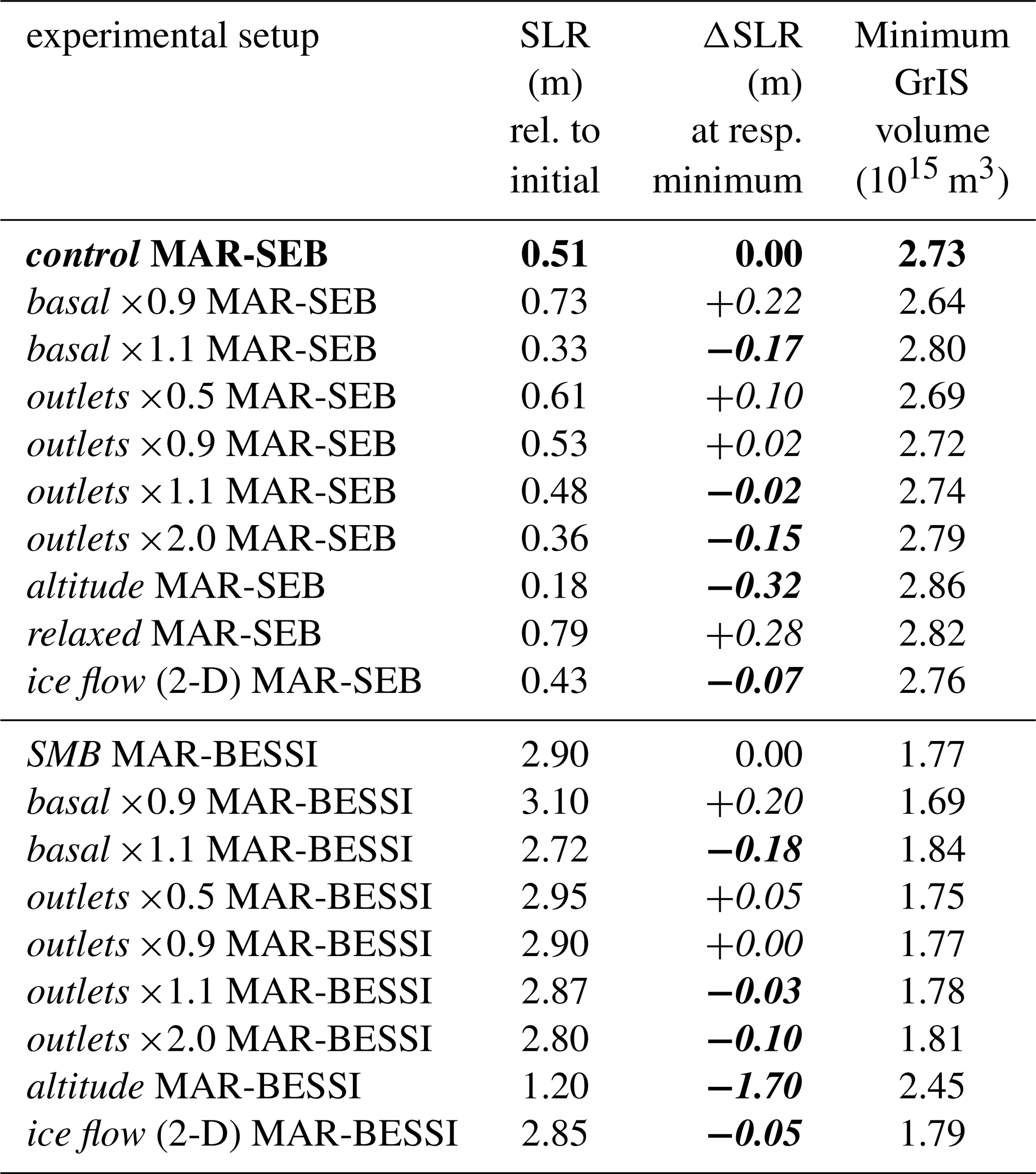
For the outlets sensitivity experiments, the basal friction in regions with >500 m yr⁻¹ is changed. Sea level rise (SLR) values are relative to the initial ice sheet at 127 ka, i.e., the modern ice sheet for all experiments except the relaxed initial ice sheet experiment. The lost ice volume is equally spread over the modern ocean area. ΔSLR refers to anomalies relative to the respective SMB forcing experiments with unchanged friction. Negative ΔSLR values are indicated in bold.

The basal experiments (thin solid lines; Fig. 1; friction $\times \mathrm{0.9}/\times \mathrm{1.1}$ for the entire ice sheet) show a stronger influence on the ice volume than the outlets experiments: changing the basal friction locally at the outlet glaciers (outlets) by factors of 0.9 and 1.1 has very little effect on the integrated ice volume (not shown). However, a halving/doubling of the friction at the outlet glaciers does show a notable effect on the ice volume (0.05 to 0.15 m at the ice minimum; thin dashed lines; Fig. 1).

The importance of the SMB–altitude feedback is illustrated in Fig. 2 which shows the evolution of the ice volume with the two SMB forcings (control, bold orange; SMB, bold purple) and without applying the SMB gradient method (altitude, thin orange/purple). Neglecting the correction of the SMB for a changing ice surface elevation, that is, using the offline calculated SMBs directly, results in significantly less melt. This is particularly pronounced in experiments forced with MAR-BESSI, because the ablation area in these simulations is larger, and therefore larger regions are affected by melt-induced surface lowering. The differences between the 3-D higher-order and the 2-D SSA are surprisingly small, particularly at the beginning of the simulations while the ice volume is decreasing (ice flow, black and gray). The differences between the ice flow approximations become larger as the ice sheet enters a colder state, at the end of the simulations. Finally, in the relaxed experiment (dark green), the volume decrease is more pronounced because the relaxed initial ice sheet is larger and the SMB forcing is negative enough to melt the additional ice at the margins. However, at the end of the simulations, the control and the relaxed experiments become indistinguishable.

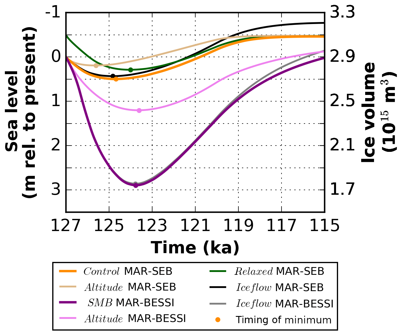
Figure 2 Evolution of the ice volume for the control (MAR-SEB, orange, bold) and the SMB experiments (MAR-BESSI, purple, bold) in comparison with the altitude, relaxed, and ice flow sensitivity experiments. The corresponding altitude (no SMB–altitude feedback) and ice flow (2-D SSA) sensitivity experiments are shown in lighter colors and black/gray, respectively. The relaxed sensitivity experiment (relaxed larger initial ice sheet but otherwise control forcing) is shown in dark green.

Comparing the SMB forcing for the control experiment (MAR-SEB; Fig. 3a–d) and the SMB experiment (MAR-BESSI; Fig. 3e–h) emphasizes the importance of the SMB–altitude feedback. While the offline calculated SMBs (using a modern ice surface) are similar, the surface lowering in combination with the SMB gradient method cause the resulting SMB to become very negative in the southwest (for both MAR-SEB and MAR-BESSI) and in the northeast (particularly for MAR-BESSI). Regions with extremely low SMB at 125 ka are ice free at the time of the simulation (ice margins are indicated with a black solid line).

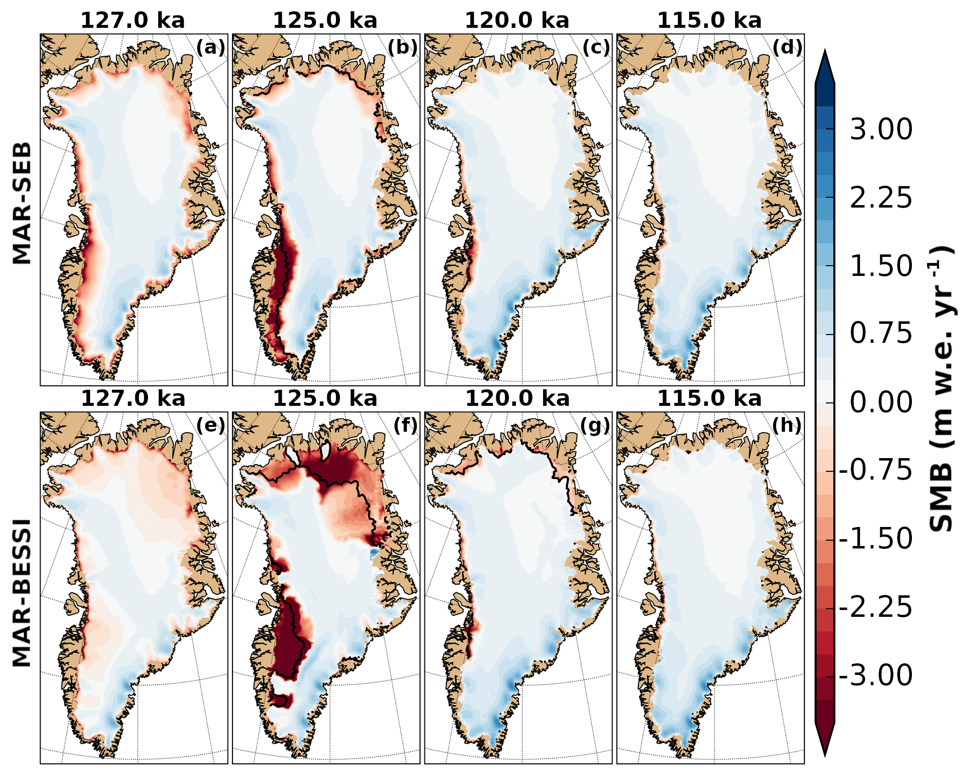
Figure 3 SMB forcing corrected for surface elevation changes at 127, 125, 120, and 115 ka for the control (a–d, MAR-SEB) and the SMB (e–h, MAR-BESSI) experiments. The ice margin is indicated with a solid black line (10 m ice thickness remaining). A nonvisible ice margin is identical to the domain margin. For a consistent comparison, the SMB is shown at 125 ka instead of the individual minimum (control at 124.7 ka and SMB at 123.8 ka).

The simulated ice sheet thickness in the control experiment (Fig. 4a–d; MAR-SEB) shows only moderate changes. However, there is a significant retreat of the ice margin in the southwest at 125 ka (Fig. 4b). The SMB sensitivity experiment (Fig. 4e–h; MAR-BESSI) on the other hand gives a very different evolution of the ice thickness: at 125 ka, the SMB experiment (Fig. 4f) shows an enhanced retreat in the southwest and additionally a particularly strong retreat in the northeast. Furthermore, the ice sheet takes longer to recover in the SMB experiment, giving a smaller ice sheet at 120 ka (Fig. 4g), mainly due to the large ice loss in the northeast.

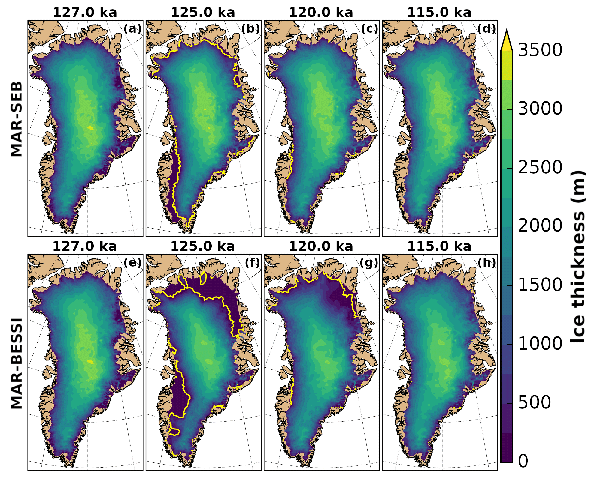
Figure 4 Ice thickness at 127, 125, 120, and 115 ka for the control (a–d, MAR-SEB) and the SMB (e–h, MAR-BESSI) experiments. The ice margin is indicated with a solid yellow line (10 m ice thickness remaining). A nonvisible ice margin is identical to the domain margin. For a consistent comparison, the ice thickness is shown at 125 ka instead of the individual minimum (control at 124.7 ka and SMB at 123.8 ka).

The MAR-SEB forced experiments give only small changes (±200 m) in ice surface elevation at the ice core locations of Camp Century, NEEM, NGRIP, GRIP, Dye-3, and East Greenland Ice-Core Project (EGRIP) (Fig. 5). At most locations, the surface elevation increases due to a positive SMB, which is not in equilibrium with the initial ice sheet. The relaxed experiment (dark green), which is in equilibrium with the initial climate, shows damped elevation changes. Notably, Dye-3 (Fig. 5c) shows the strongest initial lowering due to its southern location affected by the early Eemian warming. The MAR-BESSI-forced experiments show the largest changes in surface elevation, particularly at Dye-3 (Fig. 5c) and NGRIP (Fig. 5b) with a maximum lowering of around 600 m, and at EGRIP (Fig. 5f), where the largest lowering is around 1500 m. In contrast to the ice volume evolution, where differences between the control and the ice flow experiments are small (Fig. 2), there is a larger difference in ice surface elevation changes between the ice flow approximations. The 2-D SSA experiments (Fig. 5, black and gray) show ice surface changes up to 200 m different from the 3-D higher-order experiments (Fig. 5, bold orange and purple).

Figure 5 Ice surface evolution at Greenland ice core locations for the control, SMB, basal, outlets, ice flow, and relaxed experiments – Camp Century, NEEM, NGRIP, GRIP, and Dye-3 are shown on the same scale; EGRIP is shown on a different scale. Same color coding as in Figs. 1 and 2. Surface elevation reconstructions from total gas content at NEEM are indicated with gray shading. Note that the 2-D experiments are plotted in the background and therefore hardly visible in some cases, particularly at NEEM.

The impact of all sensitivity experiments on the ice volume minimum is summarized in Fig. 6. The choice of SMB model (SMB, black) shows the strongest influence with a difference in sea level rise of ∼2.5 m between the control experiment (with MAR-SEB) and the SMB experiment (with MAR-BESSI). Furthermore, the SMB–altitude feedback is particularly important for the MAR-BESSI-forced altitude experiment, due to the large regions affected by melt-induced surface lowering. The basal and outlets sensitivity experiments show a limited effect on the simulated ice volume minimum. Finally, using a larger, relaxed initial ice sheet (relaxed) results in a ∼0.3 m larger sea level rise. A complete summary of the respective ice volume minima is given in Table 3.

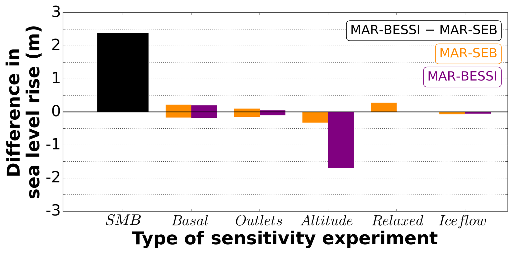
Figure 6 Differences between the minimum Eemian ice sheet simulated by the respective sensitivity experiments: SMB (black): difference between the control and the SMB experiment (MAR-SEB and MAR-BESSI, respectively); basal: experiments with changed friction for the entire ice sheet; outlets: experiments with changed friction at the outlet glaciers; altitude: experiments without the SMB–altitude feedback; relaxed: experiment with a larger, relaxed initial ice sheet; ice flow: experiments with 2-D SSA instead of the default 3-D higher-order ice flow approximation. The different SMB forcing is shown in orange (MAR-SEB) and purple (MAR-BESSI). The basal/outlets experiments show positive and negative values because they are performed with enhanced and reduced friction. The exact values are given in Table 3.

There are small differences between the simulated ice thickness minimum of the control experiment (Fig. 7a; MAR-SEB and 3-D higher-order) and the corresponding ice flow experiment (Fig. 7b; MAR-SEB and 2-D SSA). Only minor differences are visible on the east coast, where the 2-D SSA experiment shows a stronger thickening than the 3-D higher-order experiment.

Figure 7 Ice thickness anomalies simulated with the control (a; 3-D higher-order) and the ice flow (b; 2-D SSA) experiments at the respective ice minimum. Anomalies are relative to the initial modern ice sheet. The respective minimum time is indicated at the top of each panel. The ice margin is indicated with a solid black line (10 m ice thickness remaining). A nonvisible ice margin is identical to the domain margin.

Reducing the friction at the base of the entire ice sheet by a factor of 0.9 (basal ×0.9; Fig. 8b) results in a thinning on the order of 100 m in large parts of the ice sheet relative to the ice sheet minimum in the control experiment (Fig. 8a). The faster-flowing ice sheet leads to a buildup of ice at the margins and the topographically constrained outlet glaciers, particularly visible in the northeast. In contrast, reducing the basal friction only at the outlet glaciers by a factor of 0.5 (outlets ×0.5; Fig. 8c) leads to a regional thinning of several hundred meters focused around the outlet glaciers. Note that the thinning also affects ice thickness upstream from the outlet region.

Figure 8 Ice thickness of the control experiment (a), the basal ×0.9 (b; reduced friction of the entire ice sheet), and the outlets ×0.5 (c; reduced friction at outlet glaciers) experiments at their respective ice sheet minimum (time indicated at the top of the panels). Anomalies are relative to the control experiment. The ice margin is indicated with a solid yellow/black line (10 m ice thickness remaining). A nonvisible ice margin is identical to the domain margin. The outlet regions are indicated with bright green contours (c).

The ice velocities in the basal ×0.9 experiments indicate that a Greenland-wide reduction of basal friction by a factor of 0.9 leads to a speed-up of the outlet glaciers by up to several 100 m yr⁻¹ (Fig. 9b) relative to the control experiment. Furthermore, reducing the friction at the outlet glaciers by a factor of 0.5 (outlets ×0.5) results in a regional speed-up of several 100 m yr⁻¹ (Fig. 9c). Although the outlets ×0.5 experiment also shows a speed-up further upstream (on the order of several meters per year), in combination with the local ice thinning (Fig. 8c), the effects of halving the friction at the outlet glaciers show a minimal effect on the total ice volume (see also Fig. 1).

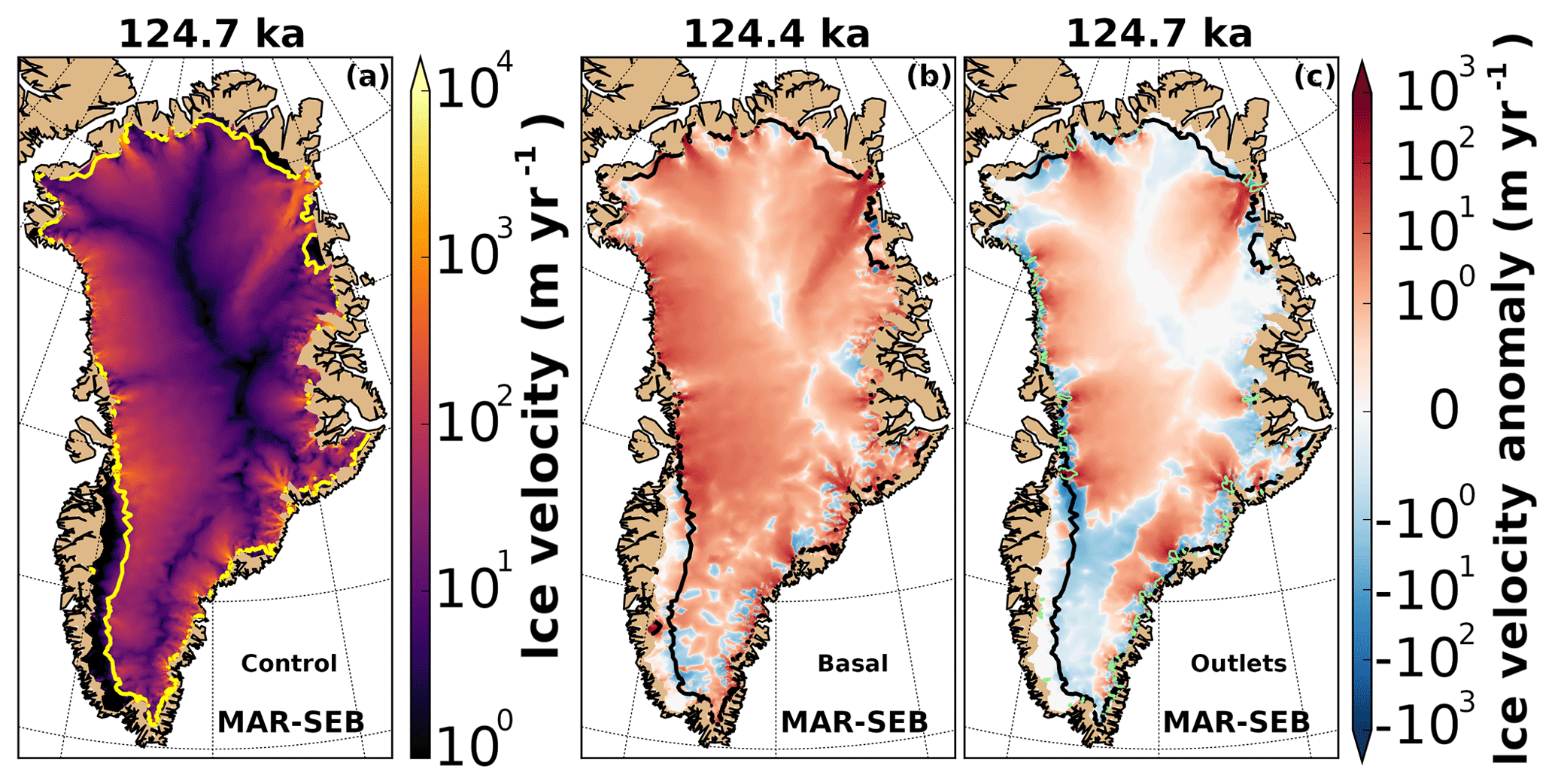
Figure 9 Ice velocity of the ice sheet in the control experiment (a) and the basal ×0.9 (b; reduced friction of the entire ice sheet), and the outlets ×0.5 (c; reduced friction at outlet glaciers) experiments at their respective ice sheet minimum (time indicated at the top of the panels). Anomalies are relative to the control experiment. The ice margin is indicated with a solid yellow/black line (10 m ice thickness remaining). A nonvisible ice margin is identical to the domain margin. The outlet regions are indicated with bright green contours (c).

4 Discussion

Changing the SMB forcing – between a full surface energy balance model (MAR-SEB) and an intermediate complexity SMB model (MAR-BESSI) – gives the largest difference in our simplified simulations of the Eemian ice sheet evolution (Fig. 6). Compromises such as the lack of ocean forcing and GIA, and limited changes of basal friction are necessary to keep 3-D higher-order millennial-scale simulations feasible and are discussed in this section.

MAR-SEB and MAR-BESSI are two estimates of Eemian SMBs selected from a wider range of simulations analyzed in Plach et al. (2018). The same Eemian global climate simulations from NorESM, downscaled over Greenland with the regional climate model MAR, are used as forcing for the SMB models. Since only one global climate model is used in this study, uncertainties related to the Eemian climate cannot be evaluated here. Instead, the reader is referred to the discussion in Plach et al. (2018).

Our control experiment with the 3-D higher-order ice flow model with modern, unchanged basal friction coefficients, and forced with MAR-SEB SMB shows minor melting (equivalent to 0.5 m sea level rise), while the SMB sensitivity experiment with MAR-BESSI SMB causes a much larger ice sheet retreat (2.9 m sea level rise; Fig. 1). The basal sensitivity experiments (basal/outlets) give an uncertainty of ±0.2 m sea level rise on top of the SMB simulations (Fig. 1); with the Greenland-wide basal friction change (basal) showing the largest influence on the minimum ice volume. Reducing/enhancing the friction at the outlet glaciers (outlets) by a factor of 0.9/1.1 shows mainly local thinning/thickening at the outlets (Fig. 8c) with limited effect on the total ice volume (Fig. 1, Table 3). However, doubling the friction at the outlet glaciers reduces the sea level rise contribution by 0.15 and 0.10 m for MAR-SEB and MAR-BESSI SMB forcing, respectively (relative to the control experiment; Table 3).

The basal friction sensitivity experiments (basal/outlets) are non-exhaustive and further experiments could be envisioned, including a lower velocity threshold to define the outlet glaciers, continuous identification of outlet regions, and combining basal ×0.9 and outlets ×0.5 experiments. In such experiments, the impact on the ice sheet evolution might be larger than in the experiments discussed. Regardless of the specific formulation of the anomalous basal friction, the sensitivity experiments shown here represent a substantial change in basal properties and they illustrate the magnitude of the uncertainties related to the basal conditions, implying that caution is required when deriving the basal friction. Finding appropriate basal conditions of past ice sheets is challenging. We show that after applying a large range of frictions it is unlikely that friction at the base has a stronger influence than changing the SMB forcing. This might be different if subglacial hydrology fed by SMB is dynamically included.

The importance of coupling climate (SMB) and ice sheet has been demonstrated in previous studies, e.g., recently for regional climate models in a projected future climate assessment by Le clec'h et al. (2019). However, running a high-resolution regional climate model over several thousand years is presently unfeasible due to the exceedingly high computational cost. This is even more true when the goal is to run an ensemble of long sensitivity simulations as presented here. Although the presented simulations are lacking the ice–climate coupling, the SMB–altitude feedback is accounted for by applying the SMB gradient method. The SMB is significantly lowered as the ice surface is lowered: neglecting the SMB–altitude feedback gives less than half the volume reduction (MAR-SEB: 0.2 vs. 0.5 m; MAR-BESSI: 1.2 vs. 2.9 m; Figs. 2 and 6).

Towards the end of the simulations, all model experiments develop a new ice sheet state which is larger than the initial state (Figs. 1 and 2). This development towards a larger ice sheet is likely related to a relaxation of the initial pre-industrial ice sheet (initial ice sheet is not in equilibrium with the initial SMB forcing) and the colder-than-present 115 ka climate. A simulation over 10 000 years with constant pre-industrial SMB gives a ∼10 % larger relaxed modern ice sheet. The relaxed sensitivity experiments with this relaxed initial ice sheet (∼0.5 m global sea level equivalent larger initial state) result in a ∼0.3 m larger sea level rise (at the minimum) compared to the control experiment. Although the 127 ka GrIS is not expected to be in equilibrium with pre-industrial forcing, the relaxed experiment demonstrates the impact of a larger initial ice sheet on our estimates of the contribution of Greenland to the Eemian sea level highstand. Furthermore, the relaxed experiment illustrates the strong, but slow, impact of the SMB forcing. Even when starting with a different initial ice sheet configuration, the final size is similar to the control experiment, because late Eemian SMB results in a steady state of the ice sheet.

Furthermore, the simplified initialization implies that the thermal structure of the simulated ice sheet is lacking the history of a full glacial–interglacial cycle; i.e., the ice rheology of our ice sheet is different from an ice sheet which is spun up through a glacial cycle. Helsen et al. (2013) demonstrate the importance of the ice rheology for the pre-Eemian ice sheet size. They find differences of up to 20 % in initial ice volume after a spin-up forced with different glacial temperatures (in simulations with basal conditions not based on assimilation of surface velocities as is the case here). In our approach, a biased thermal structure is partly compensated by basal friction optimized so that the simulated surface velocities represent the observed modern velocities. A viable way to test the influence of the thermal structure on the ice rheology would be to perform additional sensitivity experiments using a 3-D higher-order model (the 2-D SSA setup neglects vertical shear).

Starting the simulations with a smaller ice sheet would influence the simulated maximum sea level contribution. A smaller ice sheet, in combination with the SMB–altitude feedback, would result in a more negative SMB at the lower surface regions. This could potentially lead to smaller differences between the MAR-SEB and MAR-BESSI results because large regions in the MAR-BESSI simulations melted away completely, and a more negative SMB would show limited effect in such regions. However, the MAR-SEB simulations are more likely to be affected by the lower initial ice elevation. Note that neglecting GIA could counteract the effect of a lower initial ice sheet as well as a negative SMB, as the isostatic rebound of the regions affected by melt would partly compensate for the height loss.

The ice flow experiments (2-D SSA) show very similar results to the corresponding 3-D higher-order experiments (control and SMB experiments; Fig. 7). The minor differences in the east, a stronger thickening in the 2-D SSA experiments, might be explained by the complex topography in this region. The differences in ice volume between 3-D higher-order and 2-D SSA experiments (Fig. 2) become larger towards the end of the simulations under colder climate conditions (less negative SMB). Furthermore, the ice surface evolution at the ice core locations shows a similar behavior with both ice flow approximations, differences are less than ∼150 m (at most locations). The strong similarities between the 3-D higher-order and the 2-D SSA, also noted by Larour et al. (2012) using ISSM for centennial simulations are likely related to the inversion of the friction coefficients from observed velocities. The dynamical deficiencies of the 2-D SSA ice flow are partly compensated by the inversion algorithm. This algorithm chooses basal conditions such that the model simulates surface velocities as close to the observations as possible. The relatively small difference between the 3-D higher-order and 2-D SSA experiments emphasizes the controlling role of the SMB forcing and the SMB–altitude feedback in our simulations. However, ice-flow-induced thinning (for example, due to increased basal sliding) could initiate or enhance the SMB–altitude feedback.

Basal hydrology is neglected in the simulations because it is not well understood and therefore difficult to implement in a robust way. However, it is recognized that basal hydrology might have been important for the recent observed acceleration of Greenland outlet glaciers (e.g., Aschwanden et al., 2016). Therefore, the impact of changing basal conditions is tested by varying the friction at the bed of the outlet glaciers. Although basal hydrology is not explicitly simulated, its possible consequences in form of a slowdown or speed-up of the outlet glaciers is assessed (Figs. 8 and 9).

The focus of this study is on the minimum Eemian ice sheet, which has likely been land based. Our Greenland-wide simulations neglect ocean forcing and processes such as grounding line migration. Although ocean interaction is deemed an important process for marine-termination glaciers in observations (Straneo and Heimbach, 2013), a recent study presenting ocean forcing sensitivity experiments for the Eemian GrIS indicates that the Eemian minimum is governed by the atmospheric forcing, due to a lack of ice–ocean contact (Tabone et al., 2018). In contrast, the size of the glacial pre-Eemian ice sheet in their simulations is strongly influenced by the ocean heat flux and submarine melting parameter choice, implying a large impact of ocean forcing on the magnitude of ice loss over the transition into the Eemian. Our simulations, however, are initiated at 127 ka with the observed modern GrIS geometry, not with a large glacial ice sheet (following the PMIP4 protocol; Otto-Bliesner et al., 2017). Similar to Tabone et al. (2018), we therefore do not expect our smaller-than-present Eemian minimum ice sheet to be strongly sensitive to ocean forcing and conclude that the disregard of ocean forcing and processes such as grounding line migration only represents a negligible error in the magnitude of ice loss and our sea level rise estimates.

The choice of starting the simulations with the observed modern GrIS geometry is based on the fact that the present-day ice sheet is relatively well known, whereas the configuration of the pre-Eemian ice sheet is highly uncertain. Since global sea level went from a glacial lowstand to an interglacial highstand, during the course of the Eemian interglacial period, it is a fair assumption that the Eemian GrIS, at some point during this transition, resembled the present-day ice sheet. In this study, this point is chosen to be at 127 ka. One advantage of this initialization procedure is that it allows for a basal friction configuration based on inverted observed modern surface velocities. A spin-up over a glacial cycle without adapting basal friction would be unrealistic. Furthermore, a spin-up would require ice sheet boundary migration, i.e., implementation of calving, grounding line migration, and a larger ice domain. This would be challenging, as the mesh resolution is based on observed surface velocities and the domain therefore limited to the present-day ice extent. Additionally, a time-adaptive mesh, to allow for the migration of the high-resolution mesh with the evolving ice streams, would be necessary. Unfortunately, a realistic spin-up with all these additions is presently unfeasible due to the high computational cost of the model. Moreover, the lack of a robust estimate of the pre-Eemian GrIS size and the climate uncertainties over the last glacial cycle would introduce many more uncertainties to the initial ice sheet configuration.

The Eemian GrIS sea level contribution of ∼0.5 m in the control experiment is low compared to previous Eemian model studies (Fig. 10). Proxy studies based on marine sediment cores (Colville et al., 2011) and ice cores (NEEM community members, 2013) provide a sea level rise estimate of 2 m from the Greenland ice sheet during the Eemian, while assuming no contribution from the northern part of the ice sheet where no proxy constraints are available. However, scenarios with larger contributions from the north could be possible as in the MAR-BESSI-forced experiments. Although the SMB sensitivity experiment forced with SMB from MAR-BESSI shows a larger global sea level contribution of ∼3.0 m, which is closer to previous model estimates, this does not necessarily mean that the MAR-BESSI SMB is more realistic. The low sea level contribution of the control experiment could indicate systematic biases in the experimental setup, causing a general underestimation of the Eemian sea level contribution in all simulations.

Figure 10 Simulated sea level rise contributions from this study and previous Eemian studies. For this study, the results of the control (MAR-SEB; lower bound) and the SMB experiments (MAR-BESSI; upper bound) are shown (the ranges show the results of the respective basal/outlets fraction sensitivity experiments). Previous studies are color coded according to the type of climate forcing used. More likely estimates are indicated with darker colors if provided in the respective studies. A common sea level rise conversion (distributing the meltwater volume equally on Earth's ocean area) is applied to Greve (2005), Robinson et al. (2011), Born and Nisancioglu (2012), Quiquet et al. (2013), Helsen et al. (2013), and Calov et al. (2015). Tendencies of a GIA inclusion are indicated by blue arrows. The simulations of Greve (2005) were repeated with an updated ice sheet model version in 2016 (Ralf Greve, personal communication, 2016).

No GIA processes are currently included in the transient mode of ISSM. However, including rebound of the solid Earth would have the tendency to counteract the surface melting. Especially, the MAR-BESSI experiments are affected by considerable melt-induced surface lowering. The solid Earth responds in timescales of several thousand years and therefore can oppose part of the extreme surface lowering during the warmest part of the Eemian, resulting in a reduced GrIS contribution to global sea level rise. The MAR-SEB experiments show less extensive melting and less surface lowering and as a result the potential for GIA to influence the MAR-SEB SMBs is smaller. The tendencies of how the sea level rise estimates could be influenced by an inclusion of GIA are indicated by blue arrows in Fig. 10.

Both SMB models are forced with a regionally downscaled climate based on simulations with the global climate model NorESM. NorESM, as other climate models, has biases, which end up in the SMBs through downscaling procedures. This present study can be seen as a sensitivity study to SMB forcing for millennial-scale ice sheet simulations. While the simplified setup has its limits, the study emphasizes the importance of the accurate SMB forcing in general, independent of how well the presented SMBs describe the Eemian SMB. Furthermore, it is important to keep in mind that an accurate SMB forcing not only depends on the choice of SMB model but also the climate simulations used as input.

5 Conclusions

This study emphasizes the importance of an accurate surface mass balance (SMB) forcing over a more complex ice flow approximation for the simulation of the Greenland ice sheet during the Eemian. Experiments with two SMBs – a full surface energy balance model and an intermediate complexity SMB model – result in different Eemian sea level contributions (∼0.5 to 3.0 m) when forced with the same detailed regional climate over Greenland. In contrast, the comparison of experiments with 3-D higher-order and 2-D SSA ice flow gives only small differences in ice volume (<0.2 m). Furthermore, the importance of the SMB–altitude feedback is shown; neglecting this feedback reduces the simulated sea level contribution by more than 50 %. A non-exhaustive set of basal friction sensitivity experiments, affecting the entire ice sheet and only the outlet glacier regions, indicates their limited influence on the total ice volume (maximum difference of ∼0.2 m compared to experiments with default friction). While basal friction sensitivity experiments with larger impacts on the ice configuration could be envisioned, it is unlikely that such experiments would exceed the magnitude of uncertainty related to SMB. While it is challenging and arguably unfeasible at present to perform an exhaustive set of sensitivity experiments with 3-D higher-order ice flow models, cost-efficient hybrid models (SIA + SSA) could be an option to further investigate the ice dynamical processes (such as ocean forcing or basal hydrology) neglected here.

In conclusion, simulations of the long-term response of the Greenland ice sheet to warmer climates, such as the Eemian interglacial period, should focus on an accurate SMB estimate. Moreover, it is important to note that uncertainties in SMB are not only a result of the choice of SMB model but also the climate simulations used as input. Climate model uncertainties and biases are neglected in this study. However, they should be included in future Eemian ice sheet model studies in an effort to provide reliable estimates of the Eemian sea level contribution from the Greenland ice sheet.