Modelling the Antarctic Ice Sheet across the mid-Pleistocene transition – implications for Oldest Ice

The international endeavour to retrieve a continuous ice core, which spans the middle Pleistocene climate transition ca. 1.2–0.9 Myr ago, encompasses a multitude of field and model-based pre-site surveys. We expand on the current efforts to locate a suitable drilling site for the oldest Antarctic ice core by means of 3-D continental ice-sheet modelling. To this end, we present an ensemble of ice-sheet simulations spanning the last 2 Myr, employing transient boundary conditions derived from climate modelling and climate proxy records. We discuss the imprint of changing climate conditions, sea level and geothermal heat flux on the ice thickness, and basal conditions around previously identified sites with continuous records of old ice. Our modelling results show a range of configurational ice-sheet changes across the middle Pleistocene transition, suggesting a potential shift of the West Antarctic Ice Sheet to a marine-based configuration. Despite the middle Pleistocene climate reorganisation and associated ice-dynamic changes, we identify several regions conducive to conditions maintaining 1.5 Myr (million years) old ice, particularly around Dome Fuji, Dome C and Ridge B, which is in agreement with previous studies. This finding strengthens the notion that continuous records with such old ice do exist in previously identified regions, while we are also providing a dynamic continental ice-sheet context.

1 Introduction

The middle Pleistocene transition (MPT) is characterised by a shift from obliquity-driven climate cycles (∼41 000 years, 41 kyr) to the signature sawtooth ∼100 kyr cycles typical for the late Pleistocene. The drivers behind the MPT are still under debate and touch on the basic understanding of the climate system. The absence of any clear disruptive change during the MPT in orbital forcing makes the transition especially puzzling. Several theories have been put forth, striving to explain the enigmatic MPT (Raymo and Huybers, 2008). They include a shift in subglacial conditions underneath the Laurentide Ice Sheet (regolith hypothesis by Clark and Pollard, 1998), the inception of a large North American Ice Sheet (Bintanja and van de Wal, 2008) or marine East Antarctic Ice Sheet by Raymo et al. (2006), ice bedrock climate feedbacks (Abe-Ouchi et al., 2013), the buildup of large ice sheets between MIS24 and 22 identified by Elderfield et al. (2012), or the combination of changes in ice-sheet dynamics and the carbon cycle (Chalk et al., 2017). Ultimately, it seems likely that an interplay of the various proposed processes culminated in the MPT. To illuminate the potential role of these different processes and thus to solve one of the grand challenges of climate research, the recovery of a continuous ice core spanning at least beyond the MPT (in the following termed as “Oldest Ice”) is crucial. An expansion of the currently longest ice core record from the EPICA Dome C project (Jouzel et al., 2007) to and beyond the MPT would provide the necessary atmospheric boundary conditions (i.e. atmospheric greenhouse gases and surface temperature) to revisit the current theories (Fischer et al., 2013). It would provide a direct record of global atmospheric CO₂ and CH₄ concentrations and local climate during the MPT and beyond. A transient record of CO₂ concentrations would provide a key piece of the puzzle in answering the question of whether greenhouse gases were the main culprit behind the MPT, while proxies of climate conditions in Antarctica would illuminate the evolution of the Antarctic Ice Sheet leading to the MPT. However, retrieval of such an ice core is a challenging task, as a multitude of prerequisites must be met to recover an undisturbed ice core reaching more than a million years into the past (Fischer et al., 2013; Van Liefferinge and Pattyn, 2013; Parrenin et al., 2017). The European ice core community has identified a most promising target for an Oldest Ice drill site to be close to a secondary dome in the vicinity of Dome C, usually referred to as “Little Dome C” (LDC) (Parrenin et al., 2017). Also, other potential locations are targeted around Dome Fuji. The selection of sites is motivated by a series of recent studies based on radar observations of the internal ice-sheet stratigraphy and underlying bedrock topography (Young et al., 2017; Karlsson et al., 2018), local paleo-climate conditions (Cavitte et al., 2018), and 1-D and 3-D ice flow modelling (Van Liefferinge et al., 2018; Parrenin et al., 2017; Passalacqua et al., 2017). These studies provide a detailed view on the regional properties such as ice flow, thermal conditions and bedrock topography, enabling a localised assessment of promising drill sites. The only component missing so far in the analysis is the transient, continental paleo-ice-sheet dynamics perspective, which allows for the assessment of large-scale reorganisations of ice-sheet flow and geometry during glacial and interglacial cycles, their impact on divide migration, ice thickness changes along the East Antarctic ice divide and basal melt. There are many studies focussing on the transient evolution of the Antarctic Ice Sheet (AIS) during specific climate episodes in the past such as the Last Interglacial (LIG) (Sutter et al., 2016; DeConto and Pollard, 2016) or the Last Glacial Maximum (LGM) (e.g. Golledge et al., 2014). However, so far only a few studies cover the waxing and waning of the AIS during the MPT (Pollard and DeConto, 2009; de Boer et al., 2014) or late Quaternary (Tigchelaar et al., 2018) in transient model simulations with an evolving climate forcing. We build on these efforts by carrying out ensemble simulations of the Antarctic Ice Sheet across the last 2 Myr to investigate the MPT and the effect of glacial–interglacial variations in ice thickness and basal melting on potential Oldest Ice drill sites.

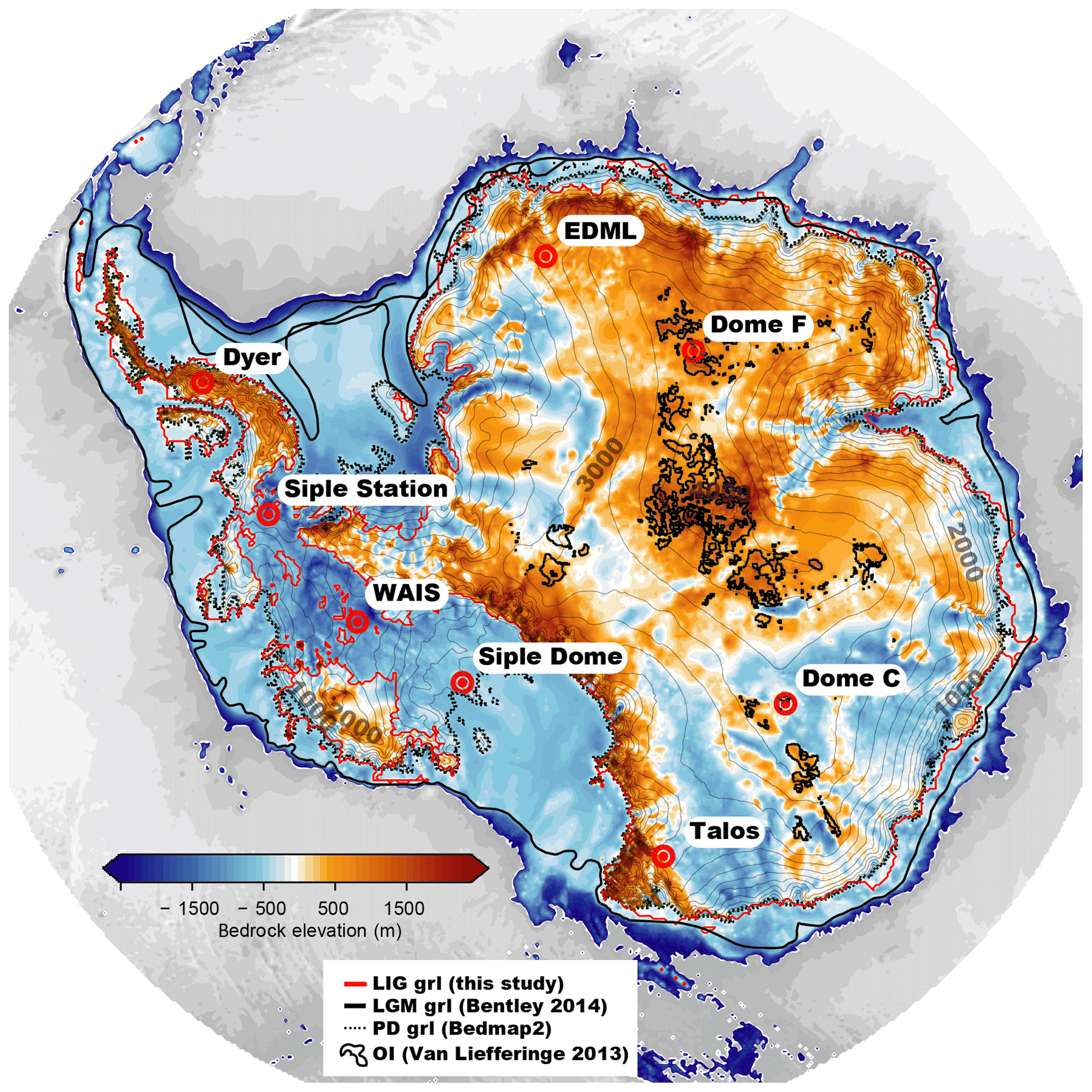
Figure 1 Antarctic bedrock topography overlain by surface contours (grey lines). The present-day (PD) grounding line (grl) from BEDMAP2 (Fretwell et al., 2013) depicted by the dashed black line. The Last Glacial Maximum (LGM) grounding line reconstruction from Bentley et al. (2014) (thick black lines) is compared to simulated grounding line retreat in one of the ensemble members for the Last Interglacial (LIG, red line). Regions previously identified as potentially viable sites for Oldest Ice (Van Liefferinge and Pattyn, 2013) are outlined by thick black lines. Eight ice core locations are highlighted, which are used as tuning targets with respect to ice core thickness and analysed in Figs. 9 (West Antarctica) and 10 (East Antarctica), respectively.

2 Methods

2.1 Ice-sheet model

We employ the 3-D thermomechanical Parallel Ice Sheet Model (PISM) (Bueler and Brown, 2009; Winkelmann et al., 2011) in the hybrid shallow-ice/shallow-shelf mode (SIA+SSA) with a subgrid grounding line parameterisation (Gladstone et al., 2010; Feldmann et al., 2014) to allow for reversible grounding line migration despite using a relatively coarse resolution. Basal sliding is calculated with a pseudo-plastic sliding law (Schoof, 2010) in which the yield stress (τ_c) is determined by the pore water content and the strength of the sediment, which is set by a linear piecewise function dependent on the ice–bedrock interface depth relative to sea level. The relevant parameter for this approach is introduced in PISM via the till-friction angle (see Winkelmann et al., 2011 Eq. 12), which is scaled linearly between till_min and till_max, depending on the bedrock elevation (see Table 2). Through this heuristic parameterisation marine-based ice has a more slippery base as compared to ice above sea level, allowing for faster flowing marine outlet glaciers. The parameter space used here yields a basal friction coefficient (e.g. underneath Thwaites glacier) on the lower end compared to Yu et al. (2018). Since the simulations presented here span a long time period (of 2 Myr), we abstain from the derivation of basal friction by inversion (optimisation problem) as we want to prevent over-tuning of present-day flow patterns. All simulations are carried out on a 16×16 km² grid and 81 vertical levels with refined resolution near the base (≈18 m at the ice–bedrock interface). The grid resolution resolves the major ice streams while allowing for reasonable computation times (ca. 100 model years per processor hour on 144 cores, i.e. ca. 5–7 d for 2 Myr depending on the supercomputer load), yet small outlet glaciers such as in the Antarctic Peninsula cannot be simulated adequately on this resolution.

The initial topography used for the simulations consists of a 200 kyr thermal spinup of the BEDMAP2 (Fretwell et al., 2013, see Fig. 1) data set (present-day steady-state simulation with fixed ice-sheet geometry), refined around LDC and Dome Fuji by the new radar-derived topographies published in Young et al. (2017) and Karlsson et al. (2018). As basal heat flux is crucial for the existence of 1.5 Myr old ice (Fischer et al., 2013; Van Liefferinge and Pattyn, 2013) as well as for ice dynamics, especially in the interior of the ice sheet (Larour et al., 2012), we consider four different geothermal-heat-flux (GHF) data sets (Shapiro and Ritzwoller, 2004; Purucker, 2013; An et al., 2015; Martos et al., 2017) in our simulations to account for uncertainties in GHF and to illustrate their impact on ice dynamics and potential Oldest Ice candidate sites.

Sea level plays an important role in the stability of marine ice sheets as it affects the position of the grounding line via the floatation criterion. We employ three different sea level reconstructions (see Sect. 2.3) to account for different glaciation patterns in the Northern Hemisphere and different sea level highstands in interglacials. PISM does not account for self-gravitational effects yet, which can have a stabilising effect on the ice sheet locally in interglacials (e.g. Konrad et al., 2014). Ice-shelf melt rates are calculated based on the parameterisation in Beckmann and Goosse (2003) (Eq. 1), with a square dependency on the temperature difference between the pressure-dependent freezing point and the ambient ocean temperature as used in Pollard and DeConto (2012),

$$\begin{array}{}\text{(1)}& M=m_{\mathrm{b}}\mathrm{0.005}{\displaystyle \frac{{\mathit{\rho }}_{\mathrm{w}}{c}_{\mathrm{pw}}}{L_i{\mathit{\rho }}_{\mathrm{i}}{\mathit{\gamma }}_{\mathrm{T}}}}\left|\right(T_{\mathrm{ocean}}^{\mathrm{3}\text{-}\mathrm{D}}-T_{\mathrm{f}}\left)\right|(T_{\mathrm{ocean}}^{\mathrm{3}\text{-}\mathrm{D}}-T_{\mathrm{f}}),\end{array}$$

where M is the melt rate in metres per second (m s⁻¹); m_b is a scaling factor; ρ_w and ρ_i are ocean water and ice-shelf density, respectively; c_pw is ocean water heat capacity; γ_T is the heat transfer coefficient; L_i is latent heat; T_f is the freezing point at depth of ice; and $T_{\mathrm{ocean}}^{\mathrm{3}\text{-}\mathrm{D}}$ is the ambient ocean temperature. The ambient ocean temperature $T_{\mathrm{ocean}}^{\mathrm{3}\text{-}\mathrm{D}}$ is derived from simple extrapolation of the 3-D ocean temperature into the ice-shelf cavity. Recently, there have been developments towards more realistic representations of basal shelf melt in stand-alone continental ice-sheet models, incorporating sub-shelf ocean circulation (e.g. Reese et al., 2018; Lazeroms et al., 2018), which improve the representation of basal ice-shelf melt rates, but they have not been included in this study. To better match present-day observed sub-ice-shelf melt rates (Rignot et al., 2013; Depoorter et al., 2013), we had to multiply the computed present-day melt rates in the Amundsen and Bellingshausen Sea by a factor of m_b=10, around the Antarctic Peninsula by 5 and underneath the Filchner Ice Shelf by a factor of 1.5. Shelf melt rates adjacent to Wilkes, Terre Adélie and George V Land in East Antarctica are also multiplied by factor of 10 in a subset of the simulations. These scaling factors are kept constant throughout the paleo-simulations. Ice-shelf calving and therefore the dynamic calving front is derived via two heuristic calving parameterisations as follows. (1) Thickness calving (cH) sets a minimum spatially uniform ice thickness (75 or 150 m) at the calving front. If the ice thickness drops below this threshold, ice in the respective grid node is purged (2) independently of 1. We additionally employ eigencalving (cE), which calculates a calving rate from the ice-shelf strain rates (Albrecht and Levermann, 2014). Both calving parameterisations are active simultaneously throughout the simulations.

2.2 Climate forcing

To adequately capture continental ice-sheet dynamics on multi-millennial timescales, in principle, a coupled modelling approach which resolves climate–ice-sheet interactions is required. First efforts to tackle multi-millennial timescales via a fully coupled modelling approach are promising and currently being developed (e.g. Ganopolski and Brovkin, 2017). However, coupled climate–ice-sheet models which resolve ice-shelf–ocean interactions are mostly limited to applications on the centennial timescale due to computational limitations. To bridge this shortcoming, we construct a transient climate forcing over the last 2 Myr by expanding time-slice snapshots from the Earth system model (ESM) COSMOS (Lunt et al., 2013) with a climate index method as applied in Sutter et al. (2016). The climate snapshots are based on Pliocene (Stepanek and Lohmann, 2012), LIG (Pfeiffer and Lohmann, 2016), LGM and pre-industrial orbital, atmospheric and topographic conditions. For each climate snapshot, anomaly fields with respect to the pre-industrial control run are calculated and added to a mean Antarctic climatology (1979–2011), derived from the regional climate model RACMO (van Wessem et al., 2014), or the extrapolated World Ocean Atlas 2009 (Locarnini et al., 2010) to provide the climate forcing for the individual climate epoch. The intermediate climate states between the snapshots are calculated by interpolating the anomaly fields with a climate index approach, utilising either of two climate indices derived from the Dome C deuterium record from Jouzel et al. (2007) which is expanded to the last 2 Myr by a transfer function (Michel et al., 2016) using the benthic oxygen isotope stack from Lisiecki and Raymo (2005) (LR04) or the global surface temperature data set from Snyder (2016). To obtain an Antarctic surface temperature record from the far field benthic oxygen isotope stack, the LR04 isotope values are scaled via

$$\begin{array}{}\text{(2)}& \begin{array}{rl}\mathrm{LR}{\mathrm{04}}_T& =-(\mathrm{LR}\mathrm{04}-\stackrel{\mathrm{‾}}{\mathrm{LR}{\mathrm{04}}_{\mathrm{810}}}){\displaystyle \frac{\mathit{\sigma }\left(\mathrm{EDC}\mathrm{2007}\right)}{\mathit{\sigma }\left(\mathrm{LR}{\mathrm{04}}_{\mathrm{810}}\right)}}\\ & +\stackrel{\mathrm{‾}}{\mathrm{EDC}\mathrm{2007}}-\mathrm{55}\mathrm{K}.\end{array}\end{array}$$

LR04_T is the new surface temperature record, LR04 is the benthic isotope stack data (time corrected to match the AICC2012 timescale; Bazin et al., 2013; Veres et al., 2013) and $\stackrel{\mathrm{‾}}{\mathrm{LR}{\mathrm{04}}_{\mathrm{810}}}$ is the mean LR04 isotope data for the last 810 kyr; standard deviations of the EDC and LR04₈₁₀ record are denoted by σ(EDC2007) and σ(LR04₈₁₀), respectively; mean Dome C surface temperature record is denoted by $\stackrel{\mathrm{‾}}{\mathrm{EDC}\mathrm{2007}}$. The forcing variables (surface temperature T_s, ocean temperature T_o) can then be calculated at every grid point in time by

$$\begin{array}{}\text{(3)}& {\displaystyle }{T}_{\mathrm{s}}^{i,j}\left(t\right)=T_{\mathrm{spd}}^{i,j}+\sum _{x=\mathrm{ig},\mathrm{g},\mathrm{p}}{\mathit{\omega }}_x\left(t\right)\mathrm{\Delta }{T}_{\mathrm{s},\mathrm{x}}^{i,j},\text{(4)}& {\displaystyle }{T}_{\mathrm{o}}^{i,j,z}\left(t\right)=T_{\mathrm{opd}}^{i,j,z}+\sum _{x=\mathrm{ig},\mathrm{g},\mathrm{p}}{\mathit{\omega }}_x\left(t\right)\mathrm{\Delta }{T}_{\mathrm{o},\mathrm{x}}^{i,j,z},\end{array}$$

where indices i,j denotes the grid point; z denotes the depth of the ice–ocean interface at grid point (i,j); $T_{\mathrm{s}}^{i,j}\left(t\right)$ is the surface temperature at grid point i,j at time t; $T_{\mathrm{spd}}^{i,j}$ is the surface temperature at present day (mean climatology from 1979–2016); and $\mathrm{\Delta }{T_{\mathrm{s}i\mathrm{g}}}^{i,j}$, $\mathrm{\Delta }{T_{\mathrm{sg}}}^{i,j}$ and $\mathrm{\Delta }{T_{\mathrm{sp}}}^{i,j}$ are the climate anomalies for the LIG, the LGM and the Pliocene, respectively. Ocean temperatures are derived in the same way (Eq. 4). The linear scaling ω_x(t) derived from the climate index (CI) interpolates the climate forcing at any given time between the respective climate states. The scaling ω_x(t) is computed by

$$\begin{array}{}\text{(5)}& {\mathit{\omega }}_{\mathrm{g}}\left(t\right)=\mathrm{1.0}-{\displaystyle \frac{\min (\mathrm{CI},{\mathrm{CI}}_{\mathrm{pd}})}{{\mathrm{CI}}_{\mathrm{pd}}}}\left\{\begin{array}{c}\mathrm{1.0}\mathrm{for}\mathrm{CI}=\mathrm{0.0}\\ \mathrm{0.0}-\mathrm{1.0}\mathrm{for}\mathrm{0.0}<\mathrm{CI}<{\mathrm{CI}}_{\mathrm{pd}}\\ \mathrm{0.0}\mathrm{for}\mathrm{CI}\mathit{⩾}{\mathrm{CI}}_{\mathrm{pd}}\end{array}\right.,\end{array}$$

$$\begin{array}{}\text{(6)}& {\mathit{\omega }}_{\mathrm{ig}}\left(t\right)={\displaystyle \frac{\left(\max \right(\mathrm{CI},{\mathrm{CI}}_{\mathrm{pd}})-{\mathrm{CI}}_{\mathrm{pd}})}{(\mathrm{1.0}-{\mathrm{CI}}_{\mathrm{pd}})}}\left\{\begin{array}{c}\mathrm{1.0}\mathrm{for}\mathrm{CI}=\mathrm{1}\\ \mathrm{0.0}-\mathrm{1.0}\mathrm{for}{\mathrm{CI}}_{\mathrm{pd}}\mathit{⩽}\mathrm{CI}\mathit{⩽}\mathrm{1.0}\\ \mathrm{0.0}\mathrm{for}\mathrm{CI}\mathit{⩽}{\mathrm{CI}}_{\mathrm{pd}}\end{array}\right.,\end{array}$$

$$\begin{array}{}\text{(7)}& {\mathit{\omega }}_{\mathrm{p}}\left(t\right)={\displaystyle \frac{\left(\max \right(\mathrm{CI},\mathrm{1.0})-\mathrm{1.0})}{({\mathrm{CI}}_{\mathrm{p}}-\mathrm{1.0})}}\left\{\begin{array}{c}\mathrm{1.0}\mathrm{for}\mathrm{CI}={\mathrm{CI}}_{\max }\\ \mathrm{0.0}-\mathrm{1.0}\mathrm{for}\mathrm{1.0}\mathit{⩽}\mathrm{CI}\mathit{⩽}{\mathrm{CI}}_{\mathrm{pd}}\\ \mathrm{0.0}\mathrm{for}\mathrm{CI}\mathit{⩽}\mathrm{1.0}\end{array}\right.,\end{array}$$

where the subscripts g, ig and p stand for glacial, interglacial and Pliocene respectively and CI_pd refers to the present-day climate index. The respective values of the climate indices are CI_lgm=0.0, CI_pd=0.70, CI_lig=1.0 and CI_p=1.13.

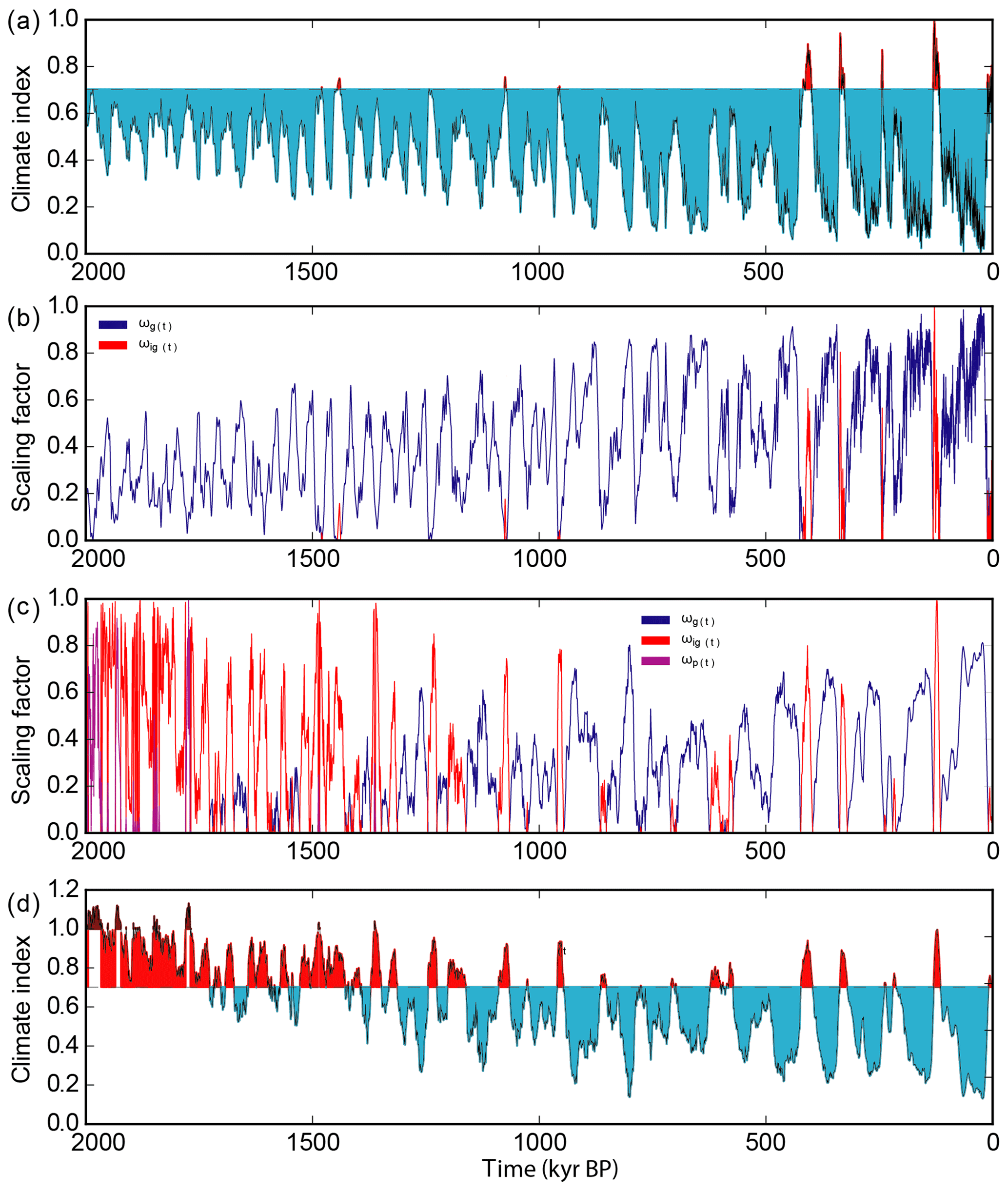
Figure 2 Climate index derived from the Dome C deuterium record (a) and corresponding scaling factors ω_x in (b). Times colder than present are shaded in cyan and times warmer than present in red. (d) same as (a) but for the climate index derived from the Snyder global surface temperature record and scaling factors ω_x in (c). Times warmer than the Last Interglacial are shaded in dark red. The lines in (b) and (c) vanish when scaling factors are zero.

The climate index is normalised with respect to the warmest climate period in the Dome C temperature record; therefore the LIG has index 1.0 in ensemble B1 and B2. The climate is linearly scaled between present day and LIG if the climate index surpasses the mean present-day climate index CI_pd and between LIG and the Pliocene if the index is larger than 1.0. The major difference between the two glacial indices is the warmer overall climate state recorded in Snyder (2016) before the MPT (see Fig. 2b). The present-day forcing derived from van Wessem et al. (2014) matches the present-day climatology in Antarctica (compared to in situ measurements) very well, with biases in the high Antarctic plateaus of less than 5 %.

We apply a temperature-dependent scaling of precipitation (P), using a scaling factor (percent precipitation change per degree Celsius) of α_P of 3 % and 5 %, respectively, motivated by central East Antarctic paleo-precipitation changes (Frieler et al., 2015; Werner et al., 2018):

$$\begin{array}{}\text{(8)}& P\left(t\right)=P_{\mathrm{pd}}+(T_{\mathrm{spd}}^{i,j}-T_{\mathrm{s}}^{i,j}(t\left)\right){\mathit{\alpha }}_{\mathrm{P}}.\end{array}$$

The precipitation is linearly dependent on the temperature anomaly with respect to present-day temperature. Note that this scaling underestimates the sensitivity of coastal mass balance to temperature changes.

In this stand-alone approach, the AIS is responding to the external forcing; thus no feedbacks are acting between the ice sheet and the climate system. However, the climate index approach implicitly incorporates the integrated climate response to changes in orbital configuration and atmospheric CO₂ archived in the Dome C (Jouzel et al., 2007), the marine sediment core (Lisiecki and Raymo, 2005) or the global surface air temperature (Snyder, 2016) record. This allows one to investigate the dynamical response of the AIS to a shifting climate regime across the MPT, with the caveat that ice-sheet–climate interactions which are not included in the GCM time-slice approach might have also played a significant role in the evolution of the AIS during the MPT.

2.3 Model ensemble approach

We choose a model ensemble approach to address the multitude of uncertainties regarding the paleo-climate state during the last 2 million years, the applied boundary conditions and the physics of ice flow. The aim of the ensemble design (Fig. 3) is to investigate the impact of different climate forcings, the response of the AIS to different geothermal-heat-flux signatures (Fig. 4) and the impact of sea level on the transient configuration of marine ice sheets. Ultimately, different manifestations of ice-sheet flow and climate response are investigated via a set of ice-sheet model parameterisations. The model parameters are preselected in equilibrium simulations under present-day forcing (1979–2011 climatology from van Wessem et al., 2014, and World Ocean Atlas Locarnini et al., 2010, ocean temperatures) trying to fit the current sea level equivalent ice-sheet volume, geometry, ice flow, ice thickness at selected ice core locations (Fig. 1) and the Antarctic sea level contribution during the last two glacial cycles. The ensemble is built around two main branches of ensemble runs consisting of a set of boundary conditions (Table 1) and ice-sheet model parameterisations (Table 2).

Figure 3 Schematic flow chart of the model ensemble. The ice-sheet model (PISM) is forced via the transient forcing derived by linear interpolation with glacial indices from Michel et al. (2016) and Snyder (2016) forming ensemble branch B1 and B2. Prescribed input data consist of sea level (SL) data and geothermal-heat-flux (GHF) data sets. Both ensemble B1 and B2 are constructed with 12 different forcing combinations (three SL data sets and four geothermal-heat-flux fields). The parameter suite is derived from sensitivity studies in which the present-day Antarctic Ice Sheet and its sea level contribution during the last two glacial cycles were the main tuning targets.

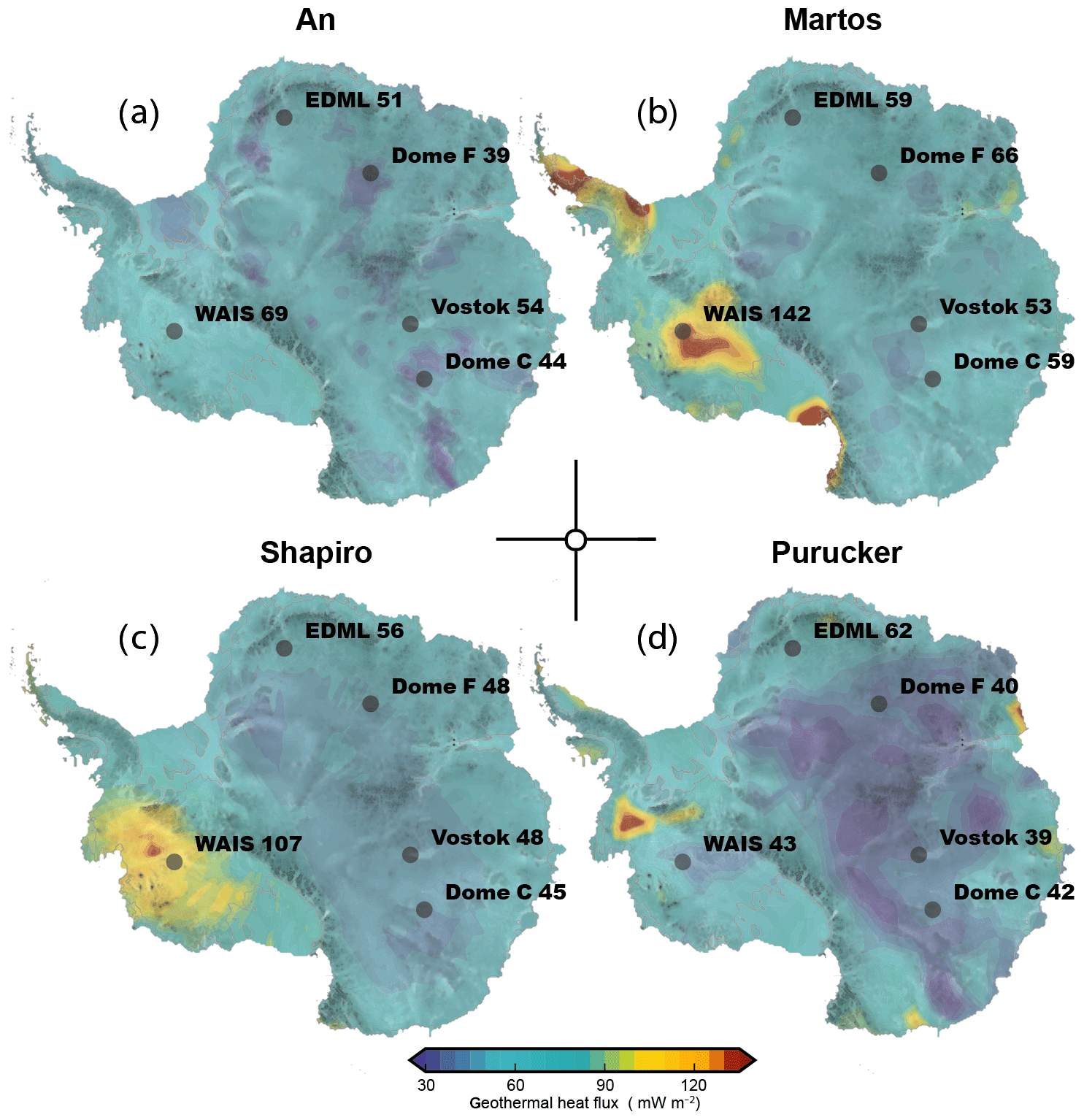
Figure 4 The four panels illustrate the four GHF input data sets (Shapiro and Ritzwoller, 2004; Purucker, 2013; An et al., 2015; Martos et al., 2017) used in this study. As a reference the rounded GHF (in mW m²) at selected ice core locations is provided.

Table 1 Available choices of selected forcing fields for the model ensemble. B1 and B2 stand for the two glacial indices derived from Michel et al. (2016) and Snyder (2016); SL data from Lisiecki and Raymo (2005) (LR05), de Boer et al. (2014) (dB14) and Rohling et al. (2014) (R14); and GHF data from Shapiro and Ritzwoller (2004) (S04), Purucker (2013) (P13), An et al. (2015) (A15) and Martos et al. (2017) (M17).

Table 2 Selected ISM parameters for the model ensemble. The first and second line show the main parameter sets used in the ensemble (P1 and P2). The third line lists additional parameters tested but not further used and discussed in this study (VP). cH stands for thickness calving limit (in metre); cE is a parameter in the eigencalving equation; sia_e and ssa_e stand for the so-called SIA and SSA enhancement factors; till_min and till_max modify basal friction in the sliding law. γ_EAIS is a dimensionless scaling factor for basal shelf melt for selected East Antarctic ice-shelf regions (George V Land, Wilkes Land). Parameter changes between P1 and P2 are highlighted in bold.

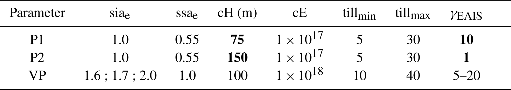
In the first ensemble branch (B1) the climate index is derived from an extrapolation of the EPICA Dome C temperature record (Jouzel et al., 2007) via correlation to the Lisiecki and Raymo (2005) time series to span the last 2 million years (Michel et al., 2016). In the second branch (B2) the climate index is derived from the global temperature record in Snyder (2016). Major differences between 2 and 0.9 Myr BP can be identified in the two resulting glacial indices. B2 exhibits much warmer climate conditions between 2 and 1.2 Myr ago. The warmest climate state in B1 is the ESM time slice centred in the LIG (MIS5) (Pfeiffer and Lohmann, 2016), while in B2 the interglacials between 2 and 1.7 Myr BP are the warmest, represented by a middle Pliocene climate time slice (Stepanek and Lohmann, 2012) (see Fig. 2). We explore two main parameter sets (P1 and P2) highlighted in Table 2. While we do take into account all sea level variations for ensemble B1, we only look at the sea level forcing derived from Lisiecki and Raymo (2005) (LR05) in ensemble B2. We also experimented with other parameter choices based on Table 2 (VP) but do not cover all individual forcing sets for these; thus they are not discussed in this study. In total we carried out 186 individual simulations. The ensemble members discussed in this paper consist of eight experiments for each ensemble B1 and B2 with sea level forcing from LR05.

3 Results and discussion

The main objective of this work is to assess the existence of 1.5 Myr old ice along the East Antarctic ice divide. We simulate the evolution of the AIS throughout the last 2 Myr, focussing on ice volume changes specifically across the MPT (see Figs. 5 and 6), as well as on ice-sheet configurations in glacials (focussing on marine isotope stage 2) and interglacials (with a focus on marine isotope stage 11 and 5; see Figs. 7 and 8). We further investigate ice thickness changes at ice core locations in West and East Antarctica (see Figs. 9 and 10). We conclude with a map of promising sites providing suitable conditions for an Oldest Ice ice core around Dome Fuji, Dome C and Ridge B, following the approach of Fischer et al. (2013) and Van Liefferinge and Pattyn (2013) (Fig. 11).

3.1 Antarctic ice volume changes

We divide our discussion of the evolution of the AIS volume into three time frames: pre-MPT (2–1.2 Myr BP), MPT (1.2–0.9 Myr BP) and post-MPT (0.8–0 Myr BP). To put our results into perspective, we compare them to two published transient ice-sheet model studies which cover the time interval considered here (Pollard and DeConto, 2009; de Boer et al., 2014) as well as Tigchelaar et al. (2018), which spans the last 0.8 Myr. Figures 5 and 6 depict the transient evolution of AIS volume as simulated by the whole ensemble and a representative subset of our model ensemble in comparison to Pollard and DeConto (2009), de Boer et al. (2014) and Tigchelaar et al. (2018) and with respect to different choices of GHF and climate index. In Fig. 6, we present two clusters of the model ensemble from branch B1 (ice/marine sediment core climate index) and branch B2 (surface air temperature climate index). Depicted are three simulations from both B1 and B2 with two model parameterisations (P1 and P2, respectively; see Table 2) using three different GHF data sets (Shapiro and Ritzwoller, 2004; Purucker, 2013; Martos et al., 2017).

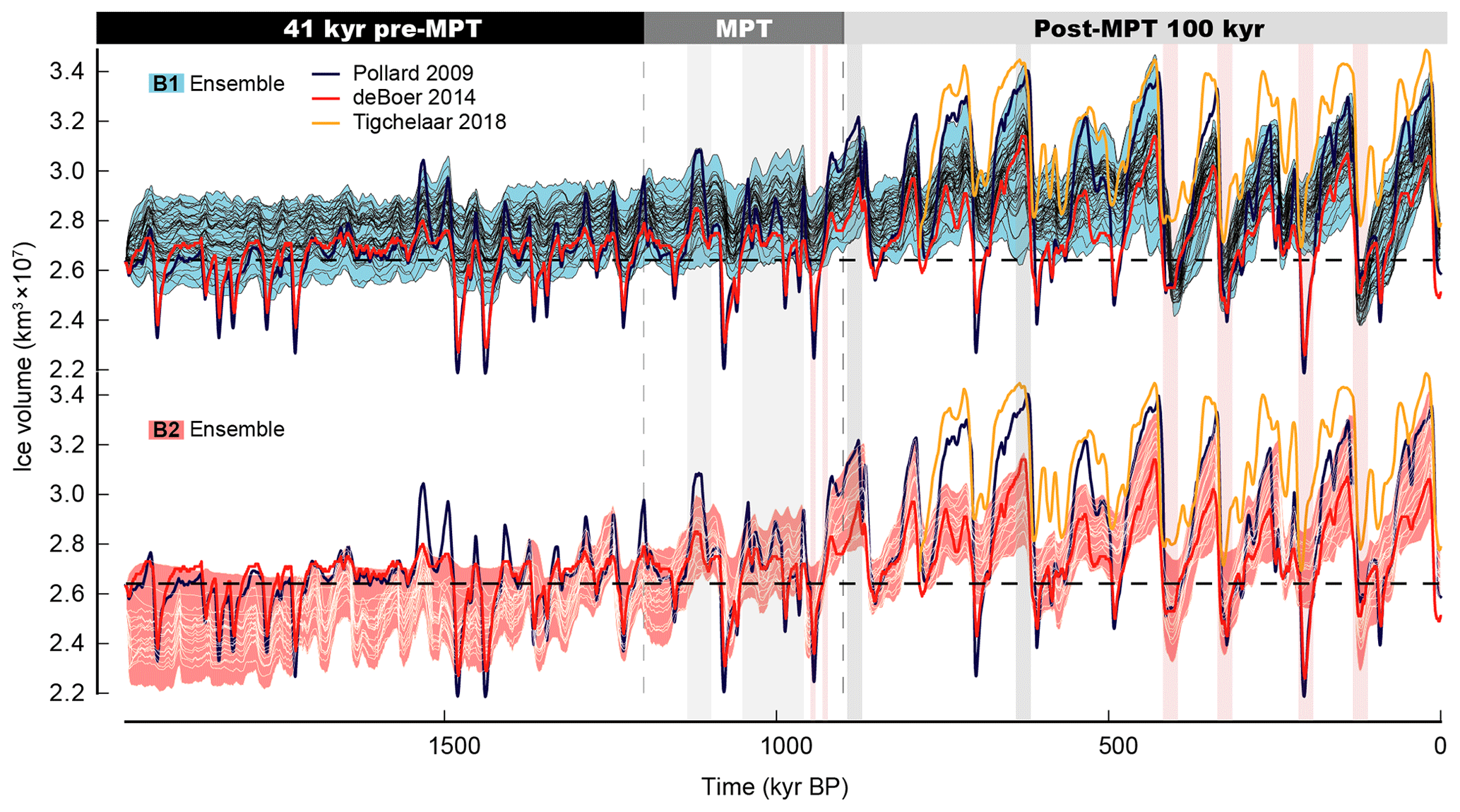
Figure 5 Antarctic ice volume as simulated in the full model ensemble (excluding simulations with either present-day ice volume larger than 2.8×10⁷ km³ or Last Glacial Maximum ice-sheet volume smaller than 3.0×10⁷ km³). The horizontal black dashed line denotes present-day ice volume derived from BEDMAP2 (Fretwell et al., 2013).

3.1.1 Pre-MPT Antarctic ice-sheet evolution

Simulated ice volume changes before the MPT are characterised by a strong obliquity (≈41 kyr) cycle resembling the climate index forcing which is formed by the integrated planetary response to orbital variations. The two clusters in the upper panel of Fig. 6 show an ice-sheet configuration similar to present day (B1 branch) and a strong interglacial configuration (B2 branch) in which the West Antarctic Ice Sheet (WAIS) has collapsed. Note that most of the ensemble members do not allow a significantly increased glaciation as encountered during the last 800 kyr. The increase in glacial AIS volume during the pre-MPT phase is limited to less than 2–4 m sea level equivalent ice volume throughout the model ensemble. Variability in the B2 branch (red) is higher than in B1 (blue), due to the waxing and waning of the marine WAIS and stronger glacial–interglacial surface mass balance variability. Ice volume in the B1 branch is predominantly driven by surface mass balance and sea level. The comparison to Pollard and DeConto (2009) and de Boer et al. (2014) illustrates the imprint of the different forcing approaches. While Pollard and DeConto (2009) and de Boer et al. (2014) both follow a combined approach using far field proxies as well as austral summer insolation (80^∘ S), we construct a transient climate forcing by combining Antarctic ESM snapshots from the Pliocene, LIG and LGM with two glacial indices derived from far field proxies. One of the main differences in our approach and the forcing applied in Pollard and DeConto (2009) and de Boer et al. (2014) is the handling of basal melting underneath the ice shelves. This forcing component arguably exerts the strongest influence on grounding line migration of the AIS in interglacials. Our calculation of basal melt rates is very similar to de Boer et al. (2014), with smaller differences between assumed peak interglacial and present-day uniform ocean temperature. Peak interglacial ocean temperatures for ensemble B1 are approximately 2 ^∘C (Last Interglacial) warmer than present day and 3 ^∘C warmer (Pliocene) in B2 (3.7 ^∘C in de Boer et al., 2014, with −1.7^∘ circum-Antarctic ocean temperatures at present day and +2^∘ at peak interglacial). Additionally, we increase the sensitivity of the basal melt rate to ocean temperature changes in certain ocean basins (see method section). Pollard and DeConto (2009) prescribe basal melt rates directly, scaling them via the far field benthic isotope record (Lisiecki and Raymo, 2005) and austral summer insolation. Ultimately, this scaling leads to larger bulk ice-shelf melt rates and smaller melt rates close to the grounding line compared to the ones calculated in our approach. Overall, this leads to a more muted ice-loss response to warmer interglacial conditions during the pre-MPT in our ensemble and a generally lower variability in ice volume (sea level equivalent of ca. 4–8 m), while the growth and retreat phases are more or less synchronous to the variations in Pollard and DeConto (2009) and de Boer et al. (2014). Interestingly, the differences in interglacial AIS volume between the three studies are largest in pre-MPT times, while they are rather similar for the last four interglacials (see Fig. 6). Evidently, the strongest interglacial AIS retreat is found in MIS7 for both Pollard and DeConto (2009) and de Boer et al. (2014), while in our ensemble it is MIS11 and MIS5, with MIS5 producing a slightly stronger response. A coherent result of our study and the results from Pollard and DeConto (2009) and de Boer et al. (2014) is that the East Antarctic Ice Sheet (EAIS) margins are relatively stable throughout the pre-MPT.

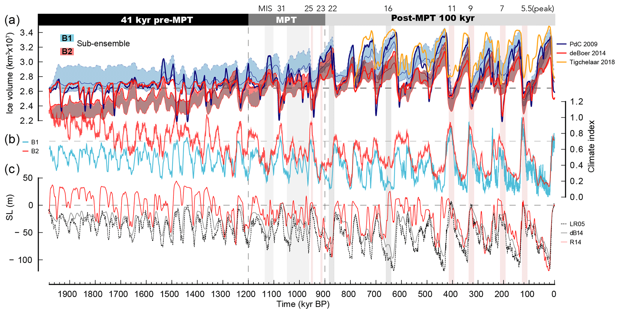
Figure 6 Panel (a) depicts the ice volume evolution of a subset of the model ensemble. Blue and light blue curves depict ensemble branch B1 with parameter set P2 (see Table 2) and sea level forcing LR04. Geothermal heat flux is depicted with the blue line (Shapiro and Ritzwoller, 2004), upper light blue dashed line (Purucker, 2013) and lower light blue line (Martos et al., 2017). The red curves show B2 with parameter set P1 and using the climate index from Snyder (2016). The red line refers to (Shapiro and Ritzwoller, 2004), the dashed maroon line refers to (Martos et al., 2017) and the maroon line refers to (Purucker, 2013). The simulated ice volume from Pollard and DeConto (2009), de Boer et al. (2014) and Tigchelaar et al. (2018) is shown for comparison (black, grey and black dashed line). (b) shows the climate index used in B1(dark grey) and B2 (light grey) with the horizontal grey dashed line depicting the average Holocene index. (c) shows the sea level reconstructions used in the model ensembles (Lisiecki and Raymo, 2005, LR04; de Boer et al., 2014, dB14; and Rohling et al., 2014, R14).

3.1.2 MPT Antarctic Ice Sheet evolution

Commonly, the onset of the MPT is put at 1.2 Myr BP and the MPT ends at about 0.9 Myr BP, culminating in extended cold conditions between marine isotope stages 24 and 22 (ca. 940–880 kyr BP). Two pronounced interglacials (MIS31 and MIS25) and several colder-than-present interglacials (between 1050 kyr and 950 kyr BP) separated by moderate glacial conditions throughout the MPT can be identified in the climate index forcing (Fig. 6b). The AIS response during the MPT is dominated by two proto-glacial states between 1.1 and 1.0 Myr BP separated by interglacial MIS31, which can be interpreted as a first expression of a 100 kyr cycle. However, obliquity pacing still dominates ice volume changes at this stage. The second proto-glacial state after MIS31 is interrupted by MIS25 followed by an extended cold period, allowing for the formation of marine ice sheets in the Weddell and Ross Sea similar to what is observed during late Quaternary glacials, marking the end of the MPT and the onset of unperturbed 80–120 kyr cycles in AIS volume. Our ice-sheet model results are in line with the notion of a 900 kyr event by Elderfield et al. (2012), which is centred around MIS25–22, manifesting itself in a qualitative difference in the formation of glacials: a long buildup phase ended by a sharp decline of the ice volume into interglacials (late Quaternary sawtooth pattern) during the last 800 kyr and a more symmetric glaciation/deglaciation before the MPT. This finding is robust across all tested sea level forcing data sets. We find no evidence of large changes in the EAIS margin during the MPT as hypothesised by Raymo et al. (2006), where a transition from a mostly land based EAIS to a marine EAIS similar to today's configuration is proposed. However, most simulations from B2, which include warm Pliocene climate conditions, show a major reorganisation of West Antarctica into a present-day ice-sheet configuration at the end of the MPT (see Fig. 9). This might represent a West Antarctic analogue to the theory that the EAIS transitioned to a marine configuration during the MPT (Raymo et al., 2006), which does not require significant changes in the EAIS margin during the MPT. Such a configurational WAIS shift would potentially implicate strong climate feedback mechanisms due to the formation of an ocean gateway between the Weddell, Ross and Amundsen Sea (Sutter et al., 2016) affecting climate dynamics across the MPT. This transition is not simulated in B1 and calls for a more crucial analysis outside the scope of this publication, e.g. incorporating a fully coupled ESM with a dynamical ice-sheet component. Accordingly, the climate state in B1 does not allow a waxing and waning of the WAIS for pre-MPT interglacial conditions. We note that other modelling studies either focussing on warmer Pliocene stages (DeConto and Pollard, 2016) or regional sensitivity studies (Mengel and Levermann, 2014) show large-scale retreat of the grounding line into the Wilkes and Aurora subglacial basins; therefore a potential reorganisation of the EAIS across the MPT cannot be excluded using all model experiments. The end of the MPT is marked by a pronounced glacial state at MIS22 akin to the Last Glacial Maximum reflecting a strong growth of the AIS at the end of the MPT. This result is robust across all ensemble members for both branch B1 and B2. It is interesting to note that the glaciations in the MPT interval become progressively stronger and reach a full late Quaternary glaciation state in MIS22.

3.1.3 Post-MPT Antarctic Ice Sheet evolution

The simulated Quaternary AIS volume evolution can be roughly divided into two parts, the first spanning the window from 900 to 420 kyr BP (MIS11) and the second from MIS11 to today. After MIS11, ice volume variability increases with smaller interglacial and bigger glacial ice sheets compared to the preceding 500 kyr. This pattern mostly reflects the stronger interglacial atmospheric and ocean temperature forcing from MIS11 onwards. MIS11 is the first late Quaternary interglacial in which the WAIS recedes to a land-based ice-sheet configuration in B1, with the second major interglacial being MIS5e. The ensemble mean sea level contribution in MIS5e amounts to ≈2.5–3 m with a full ensemble range between 1 and 4.5 m (see Fig. 8).

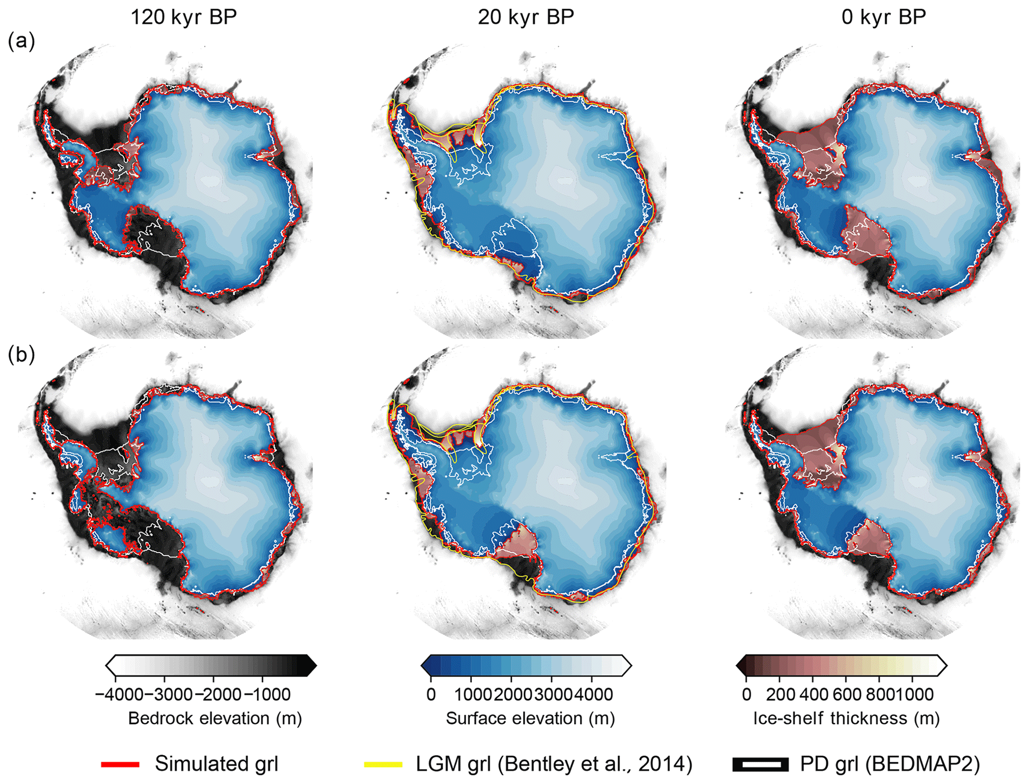
Figure 7 Panels (a–b) illustrate simulated ice-sheet configurations for the LIG, LGM and PD, respectively. Both simulations are carried out with forcing B1, using a different ice thickness calving limit (a: cH = 75 m, b: cH = 150 m). Reconstructed grounding line positions for the LGM (Bentley et al., 2014) are depicted in yellow. Both grounding line and ice-shelf front from BEDMAP2 (Fretwell et al., 2013) are depicted in white.

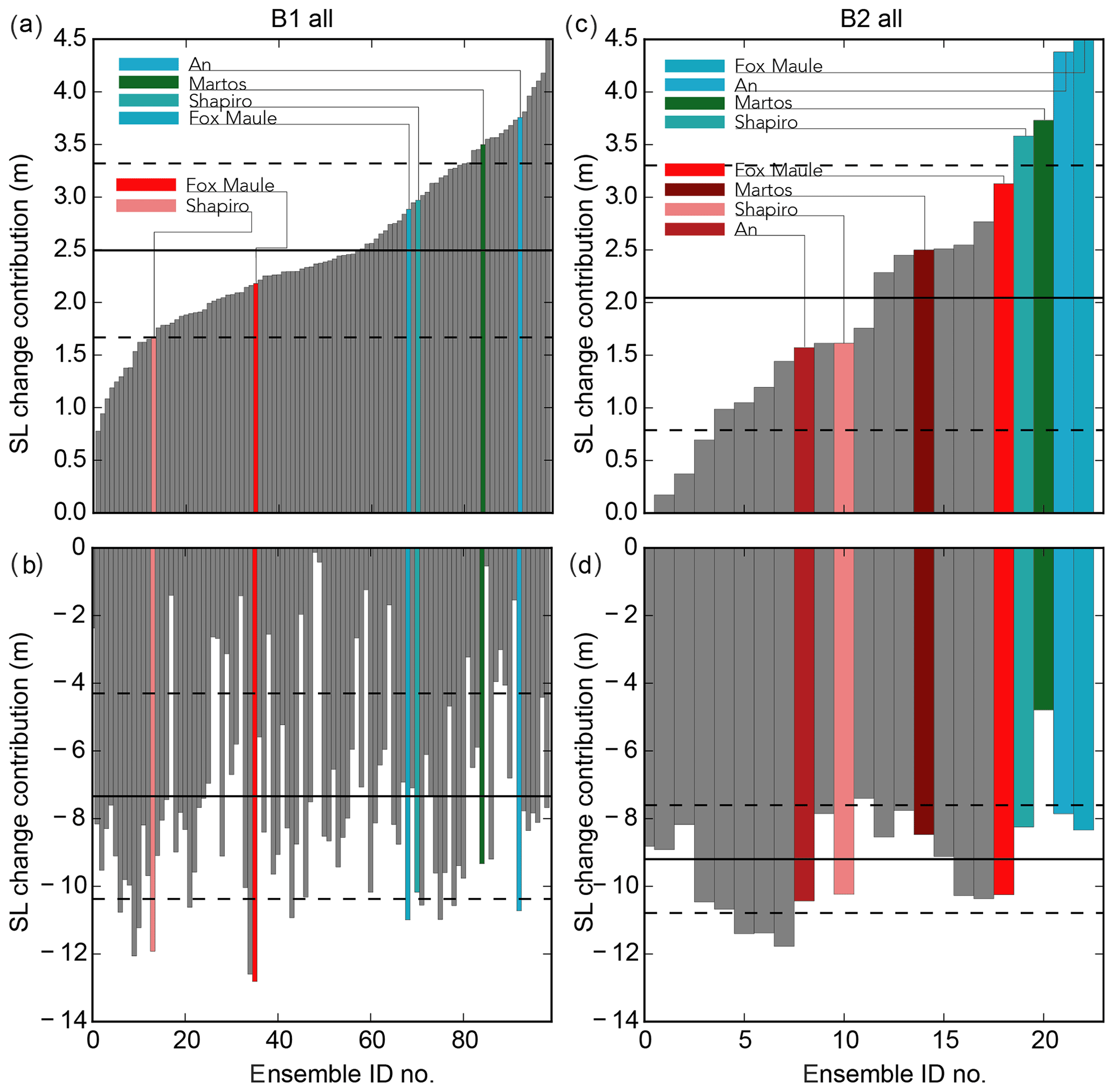
Figure 8 Sea level contribution in the LIG (a and c) and LGM (b and d) for the full ensemble forced with climate index B1 and B2. The ensemble members focused on in this paper are highlighted by colours (P1, red colours; P2, blue/green colours). Horizontal black lines depict the full ensemble means and the dashed lines the standard deviations. The x axis shows the individual ensemble IDs in ascending order of LIG SL contribution.

Glacial ice volume in the late Quaternary grows by ca. −8 to −10 m sea level equivalent ice volume (see Fig. 8), with strongest glacials represented by MIS16 and 2. In general, the glacial extent of the AIS matches reconstructed LGM grounding margins rather well, with the notable exception of the Amundsen and Bellingshausen Sea sectors. In this region, the ocean forcing seems to be too warm to allow for an advance of the ice margin to the continental shelf edge in the model. LGM ice growth in the whole ensemble is strongly dependent on the SIA enhancement factor sia_e, with values larger than 1.5 leading to an underestimation of ice thickness, albeit not necessarily ice extent. In the Ross Sea, ice thickness calving exerts a strong influence on grounding line advance. A calving thickness of 75 m generally leads to a good representation of LGM ice margin reconstructions (Bentley et al., 2014) (Fig. 7b), while simulations with a thickness limit of 150 m underestimate Ross Sea LGM grounding line advance. Furthermore, the parameterisation of ice-shelf calving can play a preeminent role in interglacials, which underlines the dire need for a physical rather than heuristic representation of calving in ice-sheet models. The different forcing approaches of our study and Pollard and DeConto (2009), de Boer et al. (2014) and Tigchelaar et al. (2018) are apparent, for example, in the largest ice-sheet retreat occurring in our ensemble at MIS5e while occurring during MIS7 (ca. 210 kyr BP) for both Pollard and DeConto (2009) and de Boer et al. (2014), whereas in Tigchelaar et al. (2018) Quaternary ice-sheet volume never drops below the present AIS volume.

3.2 The role of geothermal heat flux

It is a well established fact that the heat flux at the ice–bedrock interface can be a major driver of ice-sheet evolution. However, the GHF for the AIS is poorly constrained (Martos et al., 2017) and the few published continental data sets available differ substantially (see Fig. 4 and Martos et al., 2017). We can analyse the impact of GHF in our model ensemble by gauging the fit of diagnostic variables (ice thickness, basal melt, basal temperature, ice volume) in comparison to observed data. Both data sets from Purucker (2013) and An et al. (2015) show relatively low heat flux along the East Antarctic ice divide and overall for the WAIS. In consequence, potential Oldest Ice candidate sites indicated by the model ensemble and using those two data sets are unrealistically large, due to the absence of basal melting (see Fig. 11), specifically for the Dome Fuji region. This is the case regardless of the model parameterisation and climate forcing or sea level input data. The choice of geothermal-heat-flux imprints on both East and West Antarctic ice thickness. Modulating ice thickness (leading to thickness changes of up to 20 %) in East Antarctica also impacts the simulated ice divide along the transect of Dome A–Ridge B–Vostok–Dome C (see Fig. 11). The impact of heat flux in West Antarctica can be drastic, as it acts as a major control on the marine ice-sheet instability. All simulations with the GHF field from Purucker (2013) exhibit a collapse of the WAIS in the LIG with a much smaller percentage for both Martos et al. (2017) and Shapiro and Ritzwoller (2004). A thorough analysis of this result is beyond the scope of this paper, but it could be caused by larger glacial ice cover caused by the colder basal conditions in Purucker (2013). This would lead to an overdeepened bedrock and larger surface gradients along the coast at the onset of interglacials and therefore to favourable conditions for the marine ice-sheet instability. Overall ice-sheet variability between ensemble members (for identical parameter settings) due to different choices of GHF is consistently larger than due to the choice of different sea level forcing. This emphasises the strong role of GHF in modulating Antarctic Ice Sheet dynamics and overall evolution of ice volume.

3.3 Ice thickness variability in WAIS and EAIS

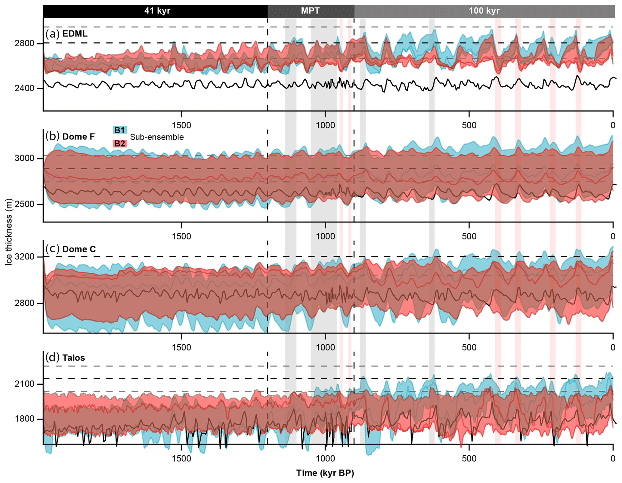
Ice thickness is an important parameter controlling the availability of a continuous 1.5-million-year-old ice core record at a given location. If the ice is too thick, its insulating properties lead to melting at the ice–bedrock interface; if it is too thin, the layering might be too thin to decipher a meaningful transient climate signal. Figures 9 and 10 show the ice thickness change at the four East and West Antarctic ice core locations which are depicted in Fig. 1.

Figure 9 Ice thickness evolution during the last 2 Myr as simulated in our model ensemble for the four West Antarctic ice core locations (see Fig. 1). Blue lines are from ensemble B1 (as in Fig. 6) and red lines from B2. Sampling rate is 1 kyr. For comparison, the ice thickness evolution simulated in Pollard and DeConto (2009) is plotted in black (sampling rate 10 kyr). The observed present-day ice thickness, derived from BEDMAP2 (Fretwell et al., 2013), is shown by the horizontal black dashed line, with 5 % variation illustrated by grey dashed lines. The ice thickness simulated in Pollard and DeConto (2009) is based on a 5 Myr transient simulation using BEDMAP1 (Lythe et al., 2001) as the initial ice-sheet configuration.

Figure 10 Same as Fig. 9 but for the four East Antarctic ice cores.

In the simulations with a collapsed late Pliocene WAIS (ensemble B2), the MPT leads to the advance of the WAIS into a present-day configuration going along with a closure of the open ocean connection between the Weddell, Amundsen/Bellingshausen and Ross Sea. However, in those simulations with no early Pleistocene WAIS, the WAIS remains relatively small throughout the Quaternary, which is likely to be an indication that the climate forcing is too warm. The ensemble members with a stable interglacial pre-MPT WAIS transition to a higher variability during the MPT with no major reorganisation of ice flow and grounding line dynamics.

Changes in the EAIS manifest in an increase in ice thickness across the MPT by ca. 30 % (mean ice thickness at ice core locations calculated for pre-MPT, 1.8–1.2 Myr BP; and Quaternary, 0.8–0.0 Myr BP) time intervals alongside an increase in variability in glacial–interglacial ice volume (standard deviation of ice thickness of individual ensemble members) of ca 50 %. The shift to larger glacial–interglacial ice thickness changes in individual ensemble members is evident at all ice core locations and mostly due to the more pronounced climate cycles following the MPT. The temporal evolution of ice thickness changes for the different East Antarctic ice core locations follows a similar pattern with muted variability during the pre-MPT and a gradual increase completed by ca. 900 kyr BP. Note that we find different points in time regarding ice thickness maxima for the central dome positions Dome C and Dome Fuji compared to positions away from the central domes such as around the EDML and Talos Dome ice core sites. While the former generally show ice-sheet maxima during mid-interglacials, the latter show maxima generally at the onset of interglacials and declining ice thicknesses during the interglacial. This and the higher glacial–interglacial variability for the two locations (EDML and Talos) can be explained by the impact of grounding line migration and larger glacial–interglacial surface mass balance differences. Mean ice thickness variability for Dome Fuji and Dome C during the late Quaternary is 165 and 195 m, respectively (105 and 140 during pre-MPT). Overall, the simulated present-day ice thickness after 2 Myr at the highlighted ice core locations in East Antarctica is in good agreement with the ice thickness derived from the BEDMAP2 (Fretwell et al., 2013) data set (within ≈5 % discrepancy in ice thickness for the selected ensemble members in B1 and B2). A notable exception is the Talos Dome ice thickness, which is too thin in all discussed B1 and B2 ensemble members except for the runs simulated with the relatively cold (Purucker, 2013) or intermediate (Shapiro and Ritzwoller, 2004) GHF data set. The applied model resolution of 16 km is generally too coarse to accurately reconstruct smaller outlet glaciers and therefore might overestimate advection away from coastal ice domes.

3.4 Mapping potential Oldest Ice sites

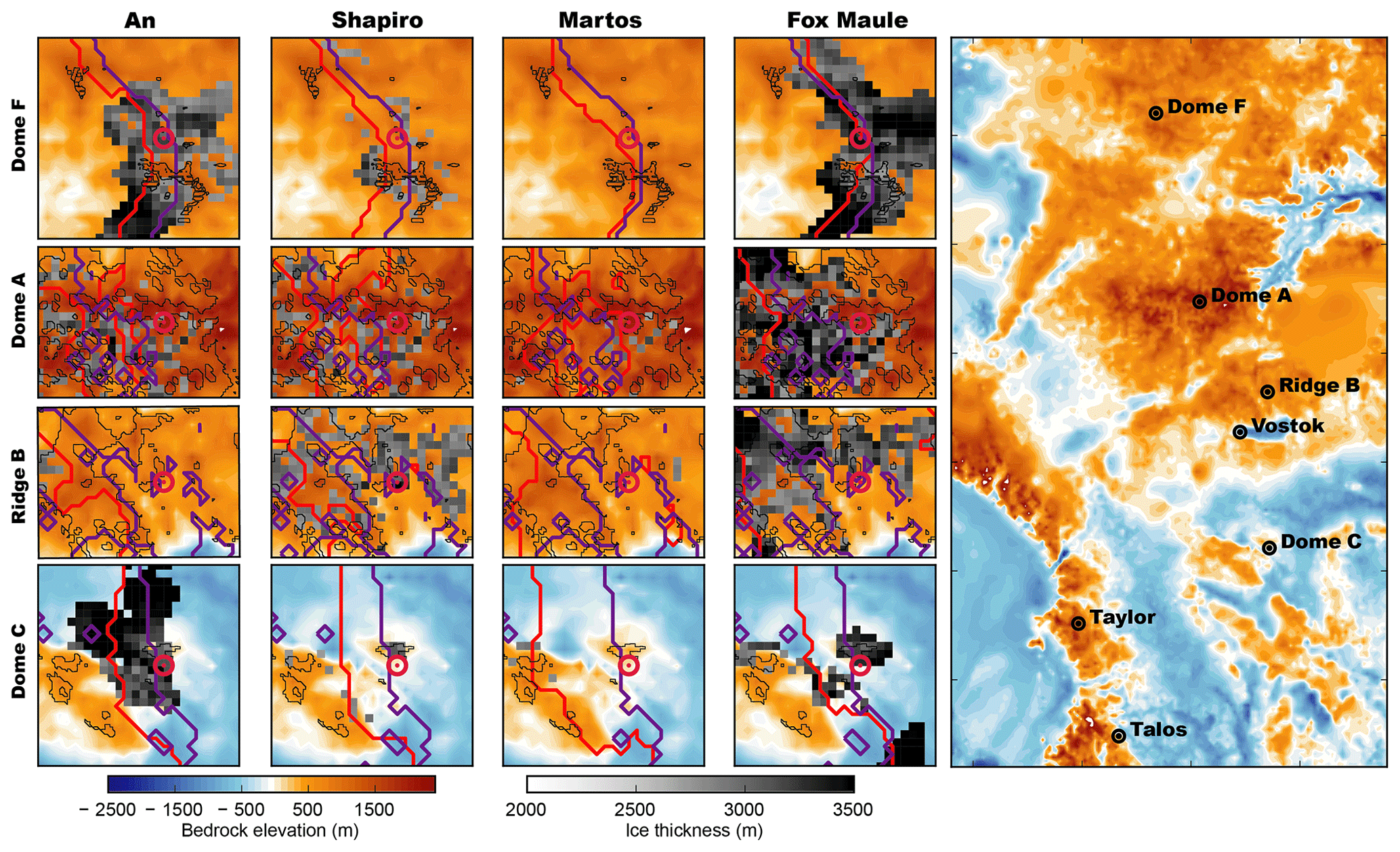
Figure 11 Comparison between regions of Oldest Ice identified in this study and in Van Liefferinge and Pattyn (2013) (Ridge B, Dome A) and Van Liefferinge et al. (2018) (Dome C, Dome Fuji) outlined by thick black lines. Regions of Oldest Ice are defined as grid nodes where ice thickness is larger than 2000 m, basal melting is zero and surface ice velocity slower than 1 m a⁻¹ (respective boxes coloured in greyscale). The left four columns show magnified sections centred at Dome Fuji, Dome A, Ridge B and Dome C for identical parameter sets and forcing but different geothermal heat flux. The respective GHF forcings used in the experiments depicted in the enlarged regions are from (left to right) An et al. (2015), Shapiro and Ritzwoller (2004), Martos et al. (2017) and Purucker (2013). The red line in enlarged regions depicts the simulated present-day ice divide (defined as position where surface elevation gradient switches direction), while the purple line depicts the present-day ice divide as computed from BEDMAP2.

We apply the conditions for the existence of 1.5 Myr old ice derived in Fischer et al. (2013) (ice thickness larger than 2000 m, basal melting zero and surface ice velocity slower than 1 m a⁻¹) to our simulations in order to investigate the impact of the transient paleo-climate forcing, GHF and different model parameterisations on the sites Dome Fuji, Dome C, Dome A and Ridge B (Fig. 11). Overall, we identify similar Oldest Ice regions as in Van Liefferinge and Pattyn (2013), Van Liefferinge et al. (2018), Parrenin et al. (2017) and Passalacqua et al. (2017). This gives us confidence in the robustness of our model results and shows that the transient forcing and continental setup used here does not change the general conclusions in Van Liefferinge et al. (2018). The regions with major overlaps to Van Liefferinge et al. (2018) are thus promising sites from a paleo-ice-climate evolution viewpoint as well as from the detailed dissection of the present-day conditions. Overall, applying the GHF from the data set by Shapiro and Ritzwoller (2004) yields the best agreement with the findings of Van Liefferinge and Pattyn (2013), Van Liefferinge et al. (2018), Parrenin et al. (2017) and Passalacqua et al. (2017). However, the geothermal-heat-flux data set from Martos et al. (2017) matches the observed/derived heat flux at Dome C to a better degree. In the simulations with the Martos et al. (2017) data set, the present-day ice divide around Dome C is shifted strongly (ca. 160 km) in the direction of the Ross Sea/Belgica Subglacial Highlands compared to the other three data sets due to the low geothermal heat flux south-west of the Dome C region contrasting with the high heat flux around Dome C (see Fig. 11). Simulations using the Martos et al. (2017) data set show almost no viable conditions for the existence of Oldest Ice in East Antarctica (with the exception of Oldest Ice patches around Dome A, Ridge B and in the Belgica Subglacial Highlands west of Dome C), as basal temperatures are relatively high due to the large heat flux at the base of the ice leading to sustained basal melting. This is the case despite the relatively low ice thickness (and therefore insulation) simulated with the Martos et al. (2017) data set. Simulations with the Purucker (2013) and An et al. (2015) GHF reconstruction overestimate the Oldest Ice area substantially (showing viable conditions also for the Dome Fuji and Dome C ice core location where subglacial melting is observed). Interestingly, however, the Purucker (2013) data sets yields the best agreement between the simulated and observed present-day ice divide for Dome Fuji as well as Dome C. The effect of the geothermal-heat-flux forcing is not limited to the basal temperature of the ice but also has a substantial impact on overall ice thickness (up to 20 % change between forcing sets; see Fig. 10, comparing the difference between simulations with different GHF in the same ensemble).

Our findings indicate that the existence of Oldest Ice is not only dependent on the choice of GHF but can also be influenced by the applied climate forcing or ice flow parameterisation modulating the regions illustrated in Fig. 11. Despite regional differences, all three sites (Dome Fuji, Dome C, Vostok/Ridge B) show suitable conditions for an Oldest Ice core throughout the last 1.5 Myr. This accounts for ensemble members using either the GHF from Shapiro and Ritzwoller (2004) or Purucker (2013) and An et al. (2015) (see Fig. 11). However the latter two show unreasonably large Oldest Ice patches. While previously identified regions of Oldest Ice (e.g. in the Dome C area; Parrenin et al., 2017) are also identified in our model results, the regions of Oldest Ice at Dome Fuji are somewhat shifted in comparison to the findings in Van Liefferinge and Pattyn (2013) and Van Liefferinge et al. (2018). This might be due to the different employed input data or ice dynamics simulated, or affected, by differences in model resolution or the thermal state at the base of the ice. However, the generally robust agreement between high-resolution studies (Van Liefferinge et al., 2018; Parrenin et al., 2017; Passalacqua et al., 2017) and our coarse-resolution paleo-dynamics approach strengthens the notion of viable conditions for Oldest Ice both at Dome Fuji and Dome C as well as Ridge B.

4 Conclusions

The search for the major drivers of the mid-Pleistocene transition is ongoing, with ice sheets acting as a crucial component of climate system rearrangement. Our model ensemble simulations indicate both rapid transitions and gradual growth of the Antarctic Ice Sheet during the MPT, featuring the buildup of a large glacial ice mass in West Antarctica driven by extended glacial conditions and muted interglacials between 1.2 and 0.9 Myr BP. These findings fit well to the notion of a significant expansion of the Antarctic Ice Sheet around 0.9 Myr BP by Elderfield et al. (2012). However, we do not find a major reorganisation of the EAIS grounding line across the MPT, which is in contrast to the theory that the EAIS transitioned from a mostly land based ice sheet to a marine configuration in this interval (Raymo et al., 2006). However, such a reorganisation cannot be excluded at this point, as several other modelling studies show potential phases of major EAIS grounding line retreat in the Pliocene or under strong interglacial conditions (DeConto and Pollard, 2016; Mengel and Levermann, 2014), and proxy reconstructions indicate large-scale EAIS grounding line retreat in the late Pleistocene (Wilson et al., 2018). While we do not simulate a transition to a marine-based EAIS in the Wilkes and Aurora basins, such a process would certainly imprint on ice flow around LDC due to proximity alone. We do find a clear transition of the WAIS configuration around 0.9 Myr in model runs where warm boundary conditions led to a collapse of the WAIS in the late Pliocene but allowed for glaciation during the colder interglacials in the MPT. We argue that such a transition between an ice-free and a present-day WAIS configuration around 900 kyr BP would have a potentially stronger influence on the global climate system (compared to an advance of the EAIS grounded ice margin) via the closing of the gateway between the Ross, Amundsen and Weddell Sea. Additionally, climate conditions favourable for a retreated configuration of the EAIS ice margin (Raymo et al., 2006) would imply a collapsed WAIS according to ice-sheet modelling studies (Golledge et al., 2015; DeConto and Pollard, 2016; Sutter et al., 2016). Our study confirms a strong contribution of the Antarctic Ice Sheet to the LIG sea level highstand, with a mean contribution of 2.5–3 m (depending on the climate index record used and the applied boundary conditions) and a maximum contribution of ca. 4.5 m, which is in line with previous studies by Golledge et al. (2015), Sutter et al. (2016) and DeConto and Pollard (2016). This corroborates the major impact of the Antarctic Ice Sheet on LIG global sea level (Dutton et al., 2015). The spatial pattern of GHF can be decisive in modelling dynamics of the WAIS. Despite this uncertainty, we identify promising candidate sites at Dome Fuji, Dome C and Ridge B which provide favourable conditions for the existence of old ice throughout the last 2 Myr. This study illustrates that uncertainties in climate forcing and boundary conditions have a large impact on paleo-climate ice-sheet simulations and therefore the assessment of Oldest Ice sites. Accordingly, the successful retrieval of an ice core spanning the last 1.5 Myr would provide a transient data benchmark and proxy horizons against which ice-sheet models can be calibrated.