the Creative Commons Attribution 4.0 License.
the Creative Commons Attribution 4.0 License.
 | 29 Mar 2019
Baffin Bay sea ice inflow and outflow: 1978–1979 to 2016–2017
Haibo Bi
Zehua Zhang
Yunhe Wang
Xiuli Xu
Yu Liang
Jue Huang
Yilin Liu
Min Fu
Baffin Bay serves as a huge reservoir of sea ice which would provide the solid freshwater sources to the seas downstream. By employing satellite-derived sea ice motion and concentration fields, we obtain a nearly 40-year-long record (1978–1979 to 2016–2017) of the sea ice area flux through key fluxgates of Baffin Bay. Based on the estimates, the Baffin Bay sea ice area budget in terms of inflow and outflow are quantified and possible causes for its interannual variations and trends are analyzed. On average, the annual (September–August) inflows through the northern gate and Lancaster Sound are on the order of km2 and km2. In particular, a comparison with published results seems to suggest that about 75 %–85 % of the inflow through the northern gates is newly formed ice produced in the recurring North Water Polynya (NOW), in addition to the inflow via Nares Strait and Jones Sound. Meanwhile, the mean outflow via the southern gate approaches km2. The distinct interannual variability for ice area flux through the northern gate and southern gate is partly explained by wind forcing associated with cross-gate sea level pressure difference, with correlations of 0.62 and 0.68, respectively. Also, significant increasing trends are found for the annual sea ice area flux through the three gates, amounting to 38.9×10³, 82.2×10³, and 7.5×10³ km2 decade−1 for the northern gate, southern gate, and Lancaster Sound. These trends are chiefly related to the increasing ice motion, which is associated with thinner ice owing to the warmer climate (i.e., higher surface air temperature and shortened freezing period) and increased air and water drag coefficients over the past decades.
- Article
(10406 KB) - Full-text XML
-
Supplement
(433 KB) - BibTeX
- EndNote


Baffin Bay is a semi-enclosed ocean basin that connects the Arctic Ocean and the northwestern Atlantic (Fig. 1). It covers an area of 630 km2 and is bordered by Greenland to the east, Baffin Island to the west, and Ellesmere Island to the north. From the north to the south, the bay spans approximately 1280 km. In the north, it connects the Arctic Ocean through Nares Straits and the channels of the Canadian Arctic Archipelago (CAA). In the south, the bay is separated from the Labrador Sea by Davis Strait (∼350 km in width). The width of the bay varies greatly, with a range of approximately 100 to 600 km.
The mean circulation of Baffin Bay is characterized by a cyclonic pattern (Fig. 1) (Melling et al., 2001; Dunlap and Tang, 2006). On the eastern side of the bay, a northward flowing West Greenland Current (WGC) along the Greenland coast carries warm and salty water from the North Atlantic. On the western side, the Baffin Current (BC) flows southward along the coast of Ellesmere and Baffin Island, bringing cold and fresh Arctic water and sea ice through Baffin Bay to Labrador Sea. Therefore, Baffin Bay serves as an important sea ice reservoir and is an important freshwater source to Labrador Sea downstream (Curry et al., 2014; Yang et al., 2016; Cuny et al., 2002). A direct potential consequence of sea ice outflow is the formation of lighter seawater that will strengthen the stratification of Labrador Sea through stabilizing the water column (Goosse et al., 1997; Rudels, 2010; Curry et al., 2014; Yang et al., 2016). These changes will potentially influence the strength of the meridional overturning circulation mechanism of the North Atlantic Ocean, which ultimately affects global deepwater circulation and exchanges (Aagaard and Carmack, 1989; Holland et al., 2001; Jahn et al., 2010; Hawkins et al., 2011; Cimatoribus et al., 2012; Yang et al., 2016).
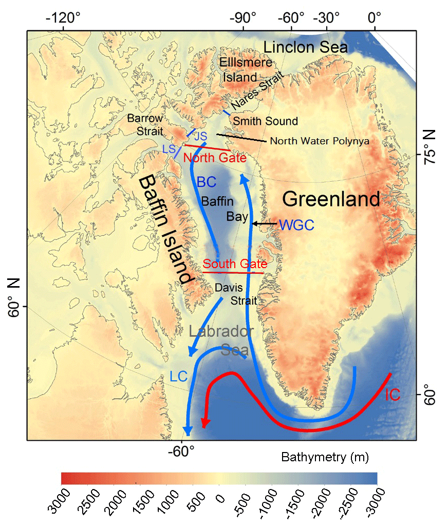
Figure 1The mean circulation pattern in Baffin Bay (blue and red arrows) and the locations of the key fluxgates to assess sea ice area flux through the bay. The West Greenland Current (WGC), Baffin Current (BC), and Labrador Current (LC) are marked with blue arrows. The Iriminger Current (IC) is represented by the red arrow. The key fluxgates through which sea ice floats into the bay includes Nares Strait, Jones Sound (JS), and Lancaster Sound (LS). Area flux through a defined northern gate together with the LS flux is used to quantify the sea ice area inflow to the bay. The outflow fields are depicted using flux via the southern gate.
Sea ice inflow and outflow have been considered to be important variables for interpreting the sea ice area balance of the Arctic Ocean (Kwok et al., 2005, 2010, 2013; Spreen et al., 2006; Kwok, 2007, 2009; Smedsrud et al., 2011; Krumpen et al., 2013, 2016; Bi et al., 2016a, b; Smedsrud et al., 2017; Zhang et al., 2017). For instance, satellite-derived sea ice export has been investigated in some key water fluxgates around the periphery of the Arctic Basin, with Fram Strait being the primary focus of study owing to its significant contribution to the changes of the Arctic sea ice extent (Smedsrud et al., 2011, 2017). In Baffin Bay, sea ice loss due to outflow through Davis Strait can be largely replenished by the inflows from the north through to the Lancaster Sound (LS), Jones Sound (JS), and Nares Strait (Fig. 1). Additionally, North Water Polynya (NOW), approximately located between Smith Sound and the northern gate (Figs. 1 and S1 in the Supplement), is deemed an important source of newly formed sea ice to the bay.
Baffin Bay sea ice inflow and outflow have significant implications for understanding the current radical climate change, because a strong atmospheric warming trend has been widely noted in the northern high latitudes (Serreze et al., 2009; Stroeve et al., 2014, 2018; Graham et al., 2017). In Baffin Bay, surface air temperature has increased by 2 to 3 ∘C decade−1 since the late 1990s (Peterson and Pettipas, 2013), resulting in prolonged days of sea ice melting there (i.e., earlier melting onset and delayed ice-freezing startup) (Stroeve et al., 2014). Accordingly, a rapid decline of sea ice coverage in all seasons has been clearly identified in the bay (Comiso et al., 2017b; Parkinson and Cavalieri, 2017). Within the context of such a pronounced climate change, examining the variability and trends in sea ice outflow through Baffin Bay over a long time series is of particular interest. Although interannual variability in sea ice inflow and/or outflow components in Baffin Bay has been reported in several studies (Cuny et al., 2005; Kwok, 2007; Curry et al., 2014), robust knowledge of their trends is necessary to predict future changes and validate model results. This study attempts to provide an extended record of the satellite-derived sea ice inflow and outflow over nearly four decades (1978–1979 to 2016–2017) through the key fluxgates of Baffin Bay and to examine the possible causes of the trends.
2.1 Data
2.1.1 Sea ice motion
The Polar Pathfinder Daily 25 km EASE-Grid Sea Ice Motion Vectors product was provided by the National Snow and Ice Data Center (NSIDC) (Tschudi et al., 2016). This product has been widely used by the modeling and data assimilation communities (http://nsidc.org/data/NSIDC-0116, last access: 27 May 2018). It is derived from a variety of sensors on satellite platforms, including the Advanced Very High Resolution Radiometer (AVHRR), Scanning Multichannel Microwave Radiometer (SMMR), Special Sensor Microwave Imager (SSM/I), Special Sensor Microwave Imager Sounder (SSMIS), and Advanced Microwave Scanning Radiometer-Earth Observing System (AMSR-E), and merged with buoy measurements from the International Arctic Buoy Program (IABP) to obtain estimates determined from the reanalyzed wind data. This study focuses on the period from November 1978 to February 2017 (Tschudi et al., 2016).
To assess the NSIDC data, a reference product of sea ice motion is employed, which is retrieved from high-resolution (∼100 m) Envisat wide-swath (∼450 km) SAR observations following methods in Kwok et al. (1990) that tracks the common ice features on image in sequence. Sea ice motion is mostly 0 %–1 % of the wind in the Arctic Ocean (Thorndike and Colony, 1982). Therefore, sea ice motion that is larger than 5 % of wind (NCEP reanalysis surface wind) is removed, since it is likely related to the tracking of weather features. A visual inspection is further conducted to identify the possible remaining erroneous ice motion fields that are not discriminated by the wind rule. Then, if the sea ice speed or direction value of a grid lying out of mean ±2 standard deviation of those of the surrounding eight grids in a 3×3 matrix, it is treated as an invalid estimate. The inverse distance interpolation method is then used to give an valid estimate for the grid.
The Envisat estimates, sampled on a 10 km grid cell, have an overall uncertainty of ∼300 m (Kwok, 2007). To facilitate a direct comparison, the spatial resolution of the derived Envisat estimates are degraded to a 25 km grid consistent with the NSIDC grids. NSIDC sea ice motion and SAR ice motion vectors in terms of drift speed (UNSIDC, USAR, in unit of km d−1) and angle (or direction) are obtained at a given location and compared. The quality of the NSIDC is examined by the following scale: sea ice speed bias (UNSIDC-USAR) (Fig. 3a) and angular (directional) difference in the sea ice drift vector (Fig. 3b). Furthermore, IABP buoy measurements of daily mean sea ice motion from January 1979 to December 1994 (http://iabp.apl.washington.edu/, last access: 1 June 2018) are used to assess the consistency of NSIDC-based sea ice area flux between 1978–1987 and later periods. There are at least 10 buoys in operation during the 1979–1994 period in the Arctic Ocean. Overall comparisons in Fig. 2 suggest that no significant difference is found with respect to the UNSIDC-USAR fields at different speed ranges between the two periods 1979–1987 (Fig. 2a) and 1988–1994 (Fig. 2b).

Figure 2Sea ice motion difference between IABP and NSIDC products at different ice drift speeds during (a) 1979–1987 and (b) 1988–1994 periods. The mean (red line) and standard deviation (error bar) of the difference at different speed ranges (from 0–6 km d−1 with a bin interval of 1 km d−1) are shown. N is the data pair number in comparison.
Two examples of Envisat ice motion fields, acquired on February 2007, are shown in Fig. 3. One example covers a cyclonic circulation along the western coast of Greenland (blue arrow, Fig. 3a) and the other is located in the area next to Davis Strait (blue arrow, Fig. 3b). Overall, comparative results (Fig. 4a) present a mean bias of −0.68 km day−1 in ice speed between the two records (i.e., slightly slower NSIDC) but a relatively large standard deviation of difference (3.11 km day−1). Furthermore, there is a small average difference of 3.4∘ in vector angle (Fig. 4b), indicating that the NSIDC motion is likely biased to the right. A large standard deviation exists in the difference in motion vector angle (38∘), which is mostly caused by data pairs for the slower Envisat motions of less than 3 km day−1 (Fig. 4b). Despite these phenomena, the two estimates agree well as a whole, as indicated by the high correlation between them (R=0.87).
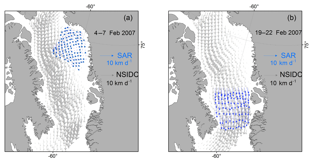
Figure 3Sea ice motion examples from NSIDC and Envisat. Gray arrows corresponds to the NSIDC data. The superimposed blue arrows, one for 4–7 February 2007 (a) and the other for 19–22 February 2007 (b), denote the corresponding Envisat estimates.
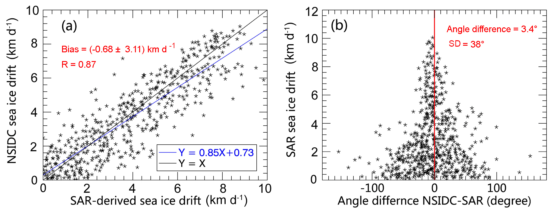
Figure 4Comparison between NSIDC ice motion and Envisat SAR estimates in terms of (a) drifting speed and (b) angular direction.
2.1.2 Sea ice concentration
Satellite-derived daily sea ice concentration records (1978–2017) were obtained from NSIDC (http://nsidc.org/data/NSIDC-0079, last access: 27 May 2018). These data are derived from the passive microwave observations from SMMR on board the Nimbus-7, the SSM/I on board the Defense Meteorological Satellite Program (DMSP) -F8, F11 and F13, and SSMIS aboard DMSP-F17 by the application of the bootstrap algorithm (Comiso et al., 2017a). For the period November 1978 to July 1987 the ice concentration is available every other day. The data gap is filled using a temporal interpolation from the data of the two adjacent days (i.e., the previous and subsequent days). The concentration field utilized here is an up-to-date version (v3.1), offering improved consistency among the estimates from the different sensors through the use of daily varying tie points. Furthermore, the product has been optimized to provide enhanced removal of weather and land contamination (Cho et al., 1996). The data are available with an equal-area grid cell structure (25 km×25 km) on a polar stereographic projection.
2.1.3 Sea ice map of the Canadian Ice Service
Weekly sea ice maps were provided by the Canadian Ice Service (CIS). As shown in Fi. S1, sea ice classification and concentration in Baffin Bay are depicted in detail on the CIS map. The CIS ice map benefits this study in the following three aspects. First, it is useful for identifying sea ice location and coverage for the NOW. Second, it enables the separation of fast ice from floating sea ice. The retrieved CIS fast ice extents are useful for detecting those coastal grid cells where ice motion should be set to zero before the calculation of sea ice area flux. As shown in Fig. 5, the eastern and western endpoint grids of the northern and southern gates, which are possibly covered by fast ice, are expected to have zero motion (see the zoomed regions marked as A, B, and C in Fig. 5). This verification serves to reduce possible systematic errors in the estimation of total area flux. In addition, the fast ice extent identified from CIS can be used to interpret the slower ice motions adjacent to the western coast of Greenland (around 75∘ N, Fig. 3). Third, the CIS map facilitates the identification of ice bridges (or ice arches), which typically form in the Nares Strait (Fig. S1). The formation of ice bridge is a common scenario during the cold freezing period in the strait and the CAA channels, which can substantially restrain Arctic sea ice inflow into Baffin Bay. Typically, two distinct bridges form: one at the northern entrance of Nares Strait adjacent to Lincoln Sea (the northern bridge) and one near the southern exit of the strait (the southern bridge, Fig. S1a). The formation of the southern bridge can fully restrict the sea ice inflow into northern Baffin Bay, as indicated by the recurring low-concentration regime just downstream of the southern bridge (Fig. S1b).

Figure 5Monthly mean fast ice extent obtained from the CIS map for the period from December 2016 to June 2017. Typical fast ice regions (a, b, and c) in Baffin Bay are zoomed to distinguish the fast ice extent during different periods. The fluxgates are also presented.
2.1.4 Reanalysis data
The reanalysis data of sea level pressure (SLP) and surface air temperature (SAT) used to analyze the impacts of climate changes on ice area flux were provided by the National Centers for Environmental Prediction/National Center for Atmospheric Research (NCEP/NCAR) (Kalnay et al., 1996). The data are available with a spatial resolution of 2.5∘ × 2.5∘.
2.2 Sea ice area flux estimation
2.2.1 Methods to estimate sea ice area flux and its uncertainty
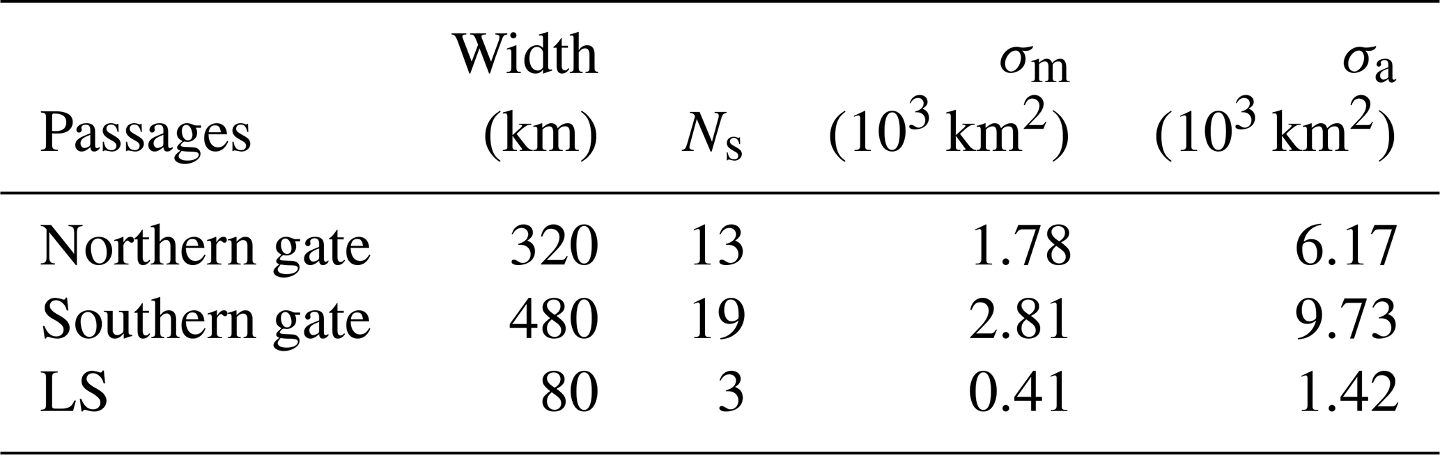
Sea ice area flux is estimated by taking the integral of the product between the gate-perpendicular component of the sea ice motion and concentration across one fluxgate (Kwok, 2007). The area fluxes through the northern gate and the Lancaster Sound (Fig. 1) are deemed the two sea ice inflow components for Baffin Bay. The northern gate (Fig. 1), spanning ∼320 km in width, is positioned at ∼75∘ N between 79 and 68∘ W, where sea ice inflow originates from three components: Jones Sound, Nares Strait, and ice produced from the NOW. Another important source of sea ice inflow is Lancaster Sound, which has a gate width of ∼80 km and can be computed with the 25 km NSIDC sea ice fields. In contrast, reliable estimates of sea ice area flux for Jones Sound and Smith Sound are not practical due to their small widths (∼40 km) with respect to the 25 km pixel resolution of the NSIDC data. Therefore, the results of several studies of the two gates are used to analyze the possible ice inflow contributions to northern Baffin Bay (see Sect. 5.1 for more details). For the outflow component, sea ice area flux is estimated across the southern gate. The gate spans ∼480 km and is located at ∼68∘ N between 63 and 53∘ W, close to Davis Strait (Figs. 1 and 5).
Before computing the area flux, the NSIDC ice motion is first interpolated to a gate to retrieve the gate-perpendicular component of ice motion. Sea ice concentration is used to weight the influences of the open water fractions on the area flux estimates. Following the trapezoidal rule, sea ice area flux (F) integrated across a fluxgate is derived as
where N is the number of along-gate grids. G corresponds to the width of a grid cell (25 km), ui is the perpendicular component of the sea ice motion, and ci is the sea ice concentration at the ith grid cell. As mentioned above, prior to the calculation, the sea ice motion fields at the endpoints of the fluxgate should be set to zero if they are covered by fast ice as recognized in the CIS maps.
The monthly sea ice area flux is calculated as the cumulative daily flux over a calendar month. Similarly, the annual flux denotes the sum of the monthly area flux of 1 year (September–August). The errors in the daily area flux estimate can be calculated as follows (Kwok, 2009): , where L is the width of the defined gate, σu is the uncertainty in daily motion and Ns is the number of independent grid cells across the gate (Table 1). For σu, we use the derived empirical error functions of mean Arctic sea-ice drift (Sumata et al., 2015). The uncertainty function is associated with sea ice concentration and speed variations, and it varies in different seasons. The uncertainty of monthly area flux is calculated as , where ND is the number of days over the month of interest. The annual flux uncertainty is calculated as , where Nm=12, i.e., the number of calendar months from September to the following August, representing a complete seasonal cycle of sea ice growth and decay. The mean uncertainties for different temporal intervals are summarized in Table 1. On average, the annual uncertainties for the northern gate, the southern gate, and LS correspond to small proportions (3.0 %, 2.5 %, and 2.6 %) of the corresponding annual mean flux estimates (provided in Sect. 4).
Table 1Mean uncertainty estimates for sea ice area flux in terms of daily (σD), monthly (σm), and annual (σa) fields for the period of 1978–1979 to 2016–2017. Ns is the number of grid cells covered by the corresponding gate.
2.2.2 Comparisons with published results
Based on SSM/I estimates of sea ice motion, Cuny et al. (2005) obtained the sea ice area flux from November to May across Davis Strait over the period 1991–1992 to 1999–2000 (Fig. 6, cyan line). During that period, sea ice area outflow was estimated to be 496×103 km2. By comparison, our NSIDC-derived flux through the southern gate (close to Davis Strait) for the same winter months of the same period is on average approximately 380×103 km2. This large difference can be mainly attributed to the distinct contrast in spatial resolution between the two sea ice motion data sets (∼70 km for the SSM/I motion data based on 37 GHz observations vs. 25 km pixels for the NSIDC data), since a larger uncertainty is expected in flux estimates based on a spatially coarser motion. The expected uncertainty in monthly flux based on SSM/I observations was computed as 6.52×10³ km2, whereas the uncertainty based on NSIDC motion is 2.27×10³ km2 (Table 1). However, the similarity of interannual behavior between the two sets of records is relatively high (R=0.56).
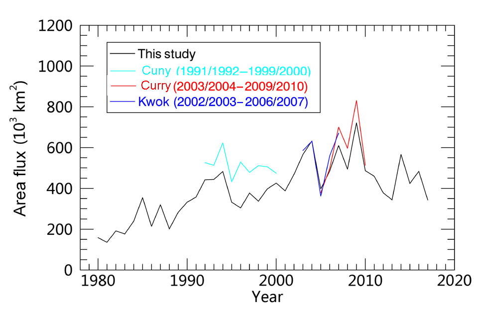
Figure 6Comparison of sea ice area flux (November to the following May) with estimates from Cuny et al. (2005), Curry et al. (2014), and Kwok (2007).
Kwok (2007) used AMSR-E data to examine sea ice drift and export in Baffin Bay over the period 2002–2003 to 2006–2007 (Fig. 6, blue). These estimates were extended to 2009–2010 in Curry et al. (2014) (Fig. 6, red). On average, our estimate of the sum of ice area flux for the November-to-May period through the southern gate is −24.3 ( km2 lower than that provided by Kwok (2007), and km2 lower than Curry's estimate (Fig. 5). Quantities after “±” are the standard deviation of the difference. Possibly, the differences are primarily caused by the differences in data inputs and are slightly due to the small differences in the locations of the defined gates among the different studies. In percentages, the biases are rather small, corresponding to small proportions (4.5 % and 8.9 %) of the average winter (November–May) estimate based on NSIDC data (511×103 km2) for the time range between 2002–2003 and 2009–2010. Moreover, good agreement between the interannual variations of the NSIDC-based results and the AMSR-E-based estimates is identified (Fig. 6). There is a high correlation of 0.93 between the NSIDC results and the AMSR-E estimates provided by Curry et al. (2014). Overall, the good consistency with the higher-resolution AMSR-E estimates suggests that the results of this study are credible.
Note that the location of the southern gate is slightly different between our study and some previous studies (Cuny et al., 2005; Curry et al., 2014) . To investigate the estimates due to the different locations of the gate, we derived the area flux through a gate further south as used in the previous studies, near to the Davis Strait (Cuny et al., 2005; Curry et al., 2014). Although the previously used gate is narrower compared to the southern gate used in this study, we found the faster ice drift there compensates for the difference in the sea ice area flux due to the flux width changes. Indeed, the NSIDC-based area flux in the southern gate (this study) and the Davis Strait gate (previous study) is quite similar (not shown).
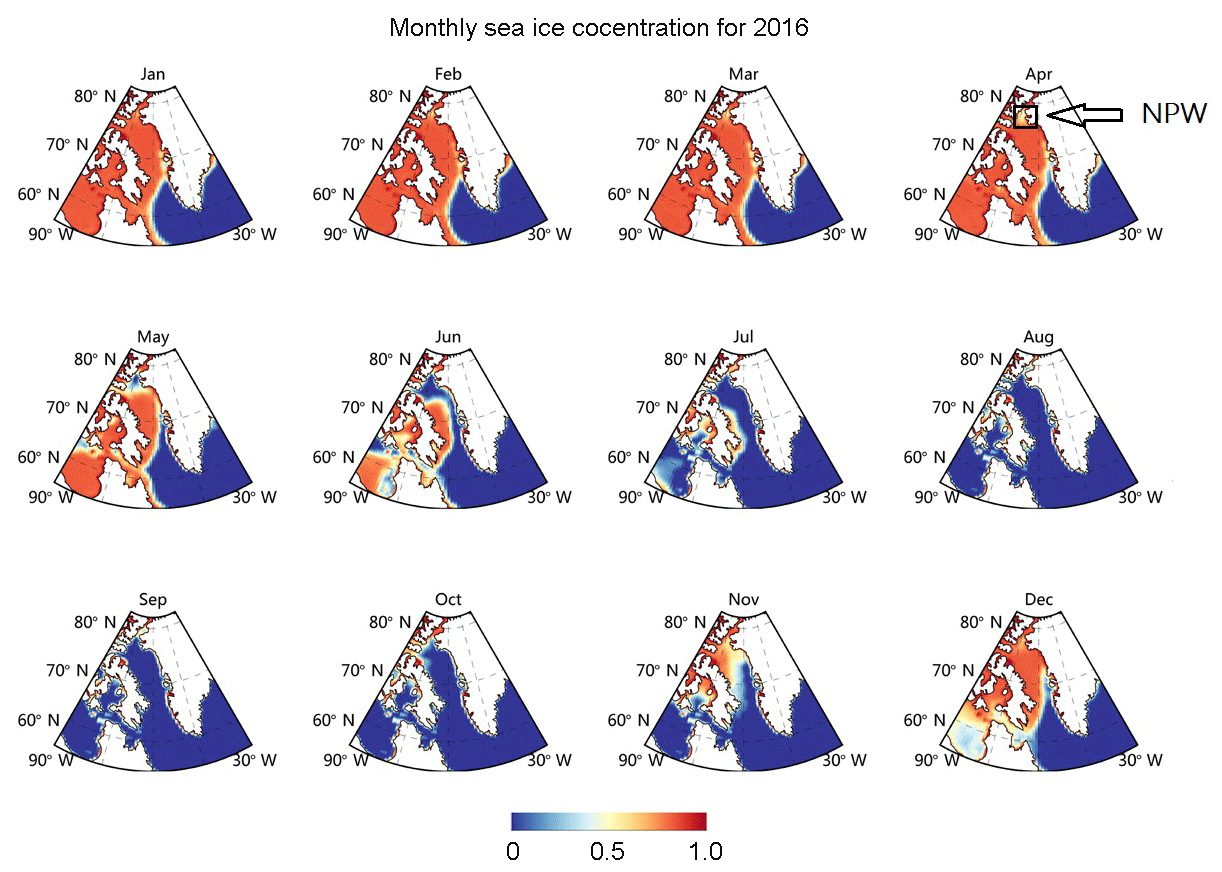
Figure 7Spatial variations of mean sea ice concentration fields for the calendar months in 2016. In the panel for April, NOW is outlined.
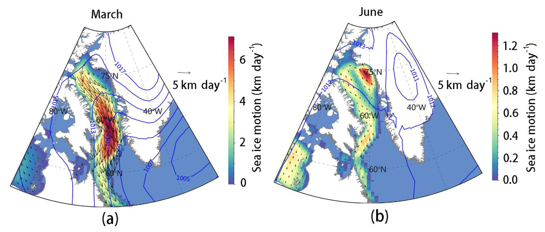
Figure 8Sea ice drift patterns (arrows) in (a) March and (b) June 2016. Background color denotes the magnitudes of sea ice speeds. Thick superimposed curves represent the SLP distribution patterns of the corresponding month.
2.3 Methods to simulate ice thickness changes and investigate the impacts on ice motion
Based on the Zubov ice growth model (, where θ is CFd−3CMd, where CFd and CMd are the cumulative degrees of SAT for freezing and melting days; for the ice growth period, CMd is set to 0), we obtain preliminary estimates of the ice thickness changes in Baffin Bay. The value of CFd for an ice growth period can be derived from the NCEP/NCAR reanalysis SAT product. To define a freezing day, we follow Stroeve et al. (2014).
Changes in sea ice thickness impact the sea ice motion fields. To assess the ice motion changes when ice thickness is altered, the standard quadratic drag laws (Eq. 2) are used to examine the ice floe acceleration due to wind (τa) and current forcing (τw) as follows:
where ρa is air density, Ca is the air–ice drag coefficient, Va is the wind velocity vector, ρa is the seawater density, Cw is the water–ice drag coefficient, Vw is the surface ocean velocity vector, ρi is the sea ice density, and hi is the ice floe thickness.
2.4 Sea ice divergence approximation
To gain further insight into the sea ice production due to the ice dynamics in Baffin Bay (see Sect. 4.2 for more details), the divergence (∇⋅V) of the sea ice motion vector field is calculated. The derivative of the ice motion field in the x and y direction is calculated by use of the Sobel operator. The Sobel operator is convolved with the x and y components Vx and Vy of the ice motion field to calculate the divergence,
where × is the convolution operator. G is the grid cell size of 25 km. The Sobel operator smoothes the field perpendicular to the derivation direction.
3.1 Sea ice coverage
The characteristic features (2016) of annual sea ice coverage of Baffin Bay are shown in Fig. 7. The bay is generally ice-free between July and October. From November, the coverage advances rapidly from the west to the east and from the north to the south. It reaches maximum coverage in late winter (March). The retreat westward around the southern gate starts in April. The southerly circulation and the warm WGC are responsible for the lower ice cover in the east of the southern gate (Fig. 1). The identifiable low sea ice concentration fields in the northern part during the cold months are associated with the occurrence of NOW (such as in April in Fig. 7).
3.2 Sea ice drift pattern
Two selected examples of sea ice drift in Baffin Bay are shown in Fig. 8. The March and June cases in 2016 are chosen to represent ice circulation under cold and warm conditions, respectively. Overall, sea ice drift in Baffin Bay is characterized by a cyclonic pattern. To the west, the sea ice motion (Fig. 8a) is connected to the northerly Baffin Current (BC, Fig. 1). To the east, the slower drift (Fig. 8a) and even southerly drift (Figs. 8b and 3), especially in the northeastern corner of the bay (around 75∘ N), are associated with the southerly West Greenland Current (WGC, Fig. 1).
In March, the prevailing drift pattern in the bay is southward (Fig. 8a). Sea ice starts from Smith Sound and the southern end of Nares Strait and extends southward along the coast of Baffin Island. From the northern end of the bay to Davis Strait, the sea ice motion gradually accelerates, reaching maximum speeds around Davis Strait (Fig. 8a). The mean sea ice speed in the northern gate is 3.2 km day−1, whereas sea ice in the southern gate attains a speed of 8.5 km day−1. Moreover, the CIS map demonstrates that the thicker multiyear ice from the Arctic through either the Nares Strait (Fig. S1a) or Lancaster Sound (Fig. S1b) is mostly confined to the west of the bay. In contrast, most of the ice motion fields in June have decreased sharply to less than 0.8 km day−1, but the basin-scale cyclonic pattern is still observable (Fig. 8b).
The general cyclonic sea ice movement pattern can be attributed to the wind forcing associated with the SLP distribution (blue curved lines in Fig. 8). The associated denser isobars in the bay imply a stronger geostrophic wind flow in March (Fig. 8a). The deep SLP trough (as apparent in March, Fig. 8a) begins to emerge in October (not shown) and is gradually enhanced until the end of March. The trough enters a weak stage from April to the end of summer, as evident in June in Fig. 8b. The spatial distribution of the trough in June is responsible for the remarkable features of ice circulation, such as the southeasterly flows in the northeastern part of the bay and the northwesterly flows in Davis Strait (Fig. 7b). Owing to modulation by the structure of the coastline, the actual sea ice drift direction in the bay tends to be on the right of the isobars (Fig. 8a).
3.3 Trends in sea ice motion and concentration fields
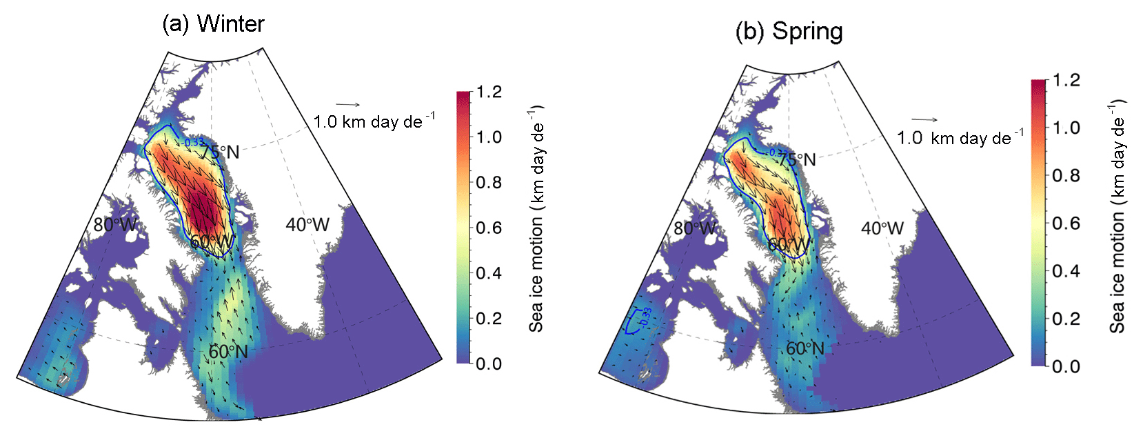
During cold seasons over the period 1978–1979 to 2016–2017, the sea ice concentration fields in Baffin Bay show a basin-scale average declining trend ranging from −1.2 % decade−1 (winter, December–February, Fig. 9a) to −3.1% decade−1 (spring, March–May, Fig. 9b). During the warm seasons (summer: June–August; autumn: September–November), the sea ice decrease is stronger, with an average change rate of −10.4 % (not shown). Clear regional variations in the trend fields are apparent in Fig. 9. Around the southeastern edge during the winter period, sea ice retreats northward and eastward, with a significant decreasing trend in ice concentration, in excess of −10 %, relative to the 2.8 % decade−1 decline reported earlier along this edge for the period 1951–2001 (Stern and Heide-Jørgensen, 2003). However, sea ice concentration in other regions of the bay shows a quite declining trends weaker than −2.0 % decade−1 (Fig. 9a).
A small enclosed area of the NOW region at the northern end of the bay also displays a declining trend in sea ice concentration fields (Fig. 9a and b). In the NOW region, there is an average sea ice concentration decrease in winter (−3 % decade−1) and a stronger decrease during spring (−8 % decade−1). This seasonal difference is primarily associated with the appearance of the ice bridge near the Smith Sound in late winter or early spring (February or March). More new ice can be produced from NOW during the spring period than the winter, and the recurring ice bridge can largely recede into the ice inflow from the Nares Strait into Baffin Bay. Therefore, higher fractions of the sea ice inflow component originating from NOW production seem to occur in spring than in winter. The more recently produced ice thus contributes to the observed fields of lower concentration in the NOW region in spring (Fig. 9b). Additionally, the decline in sea ice concentration in the NOW seems to be partially associated with the southward sea ice motion (Fig. 10a and b). In the broad regions just south of the NOW, the increased southward ice advection provides more chances for the creation of newly formed ice in polynyas. Therefore, the enhanced southward ice advection through Baffin Bay (∼1.0 km d−1 decade−1) may also have contributed to the decrease in ice concentration over the NOW regime.
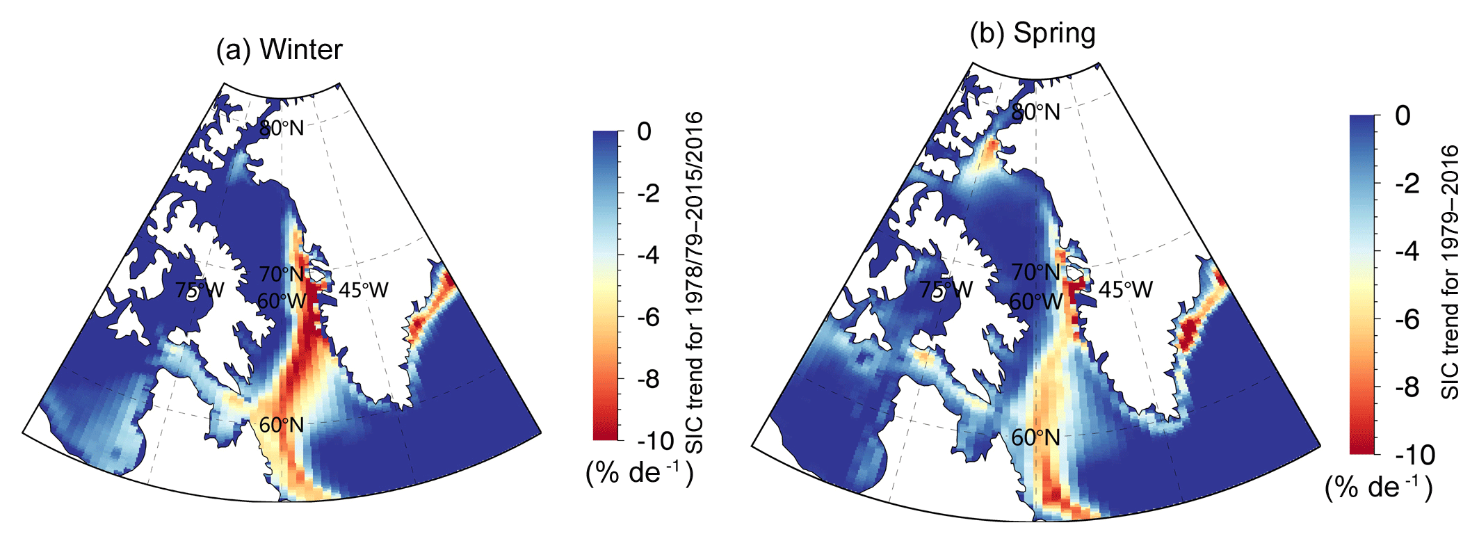
Figure 9Sea ice concentration trends during (a) winter and (b) spring over the period 1978–1979 to 2016–2017.
In this study, sea ice area flux across three gates is obtained. Sea ice inflows to the bay are measured across the northern gate and Lancaster Sound, and the sea ice outflow is estimated across the northern gate (Fig. 5). The obtained sea ice flow budget (outflow-inflow) provides knowledge of sea ice production or loss associated with the dynamic and thermodynamic processes in the regions between the northern and southern gates.
4.1 Monthly variability of sea ice area flux
Figure 11 shows the monthly mean sea ice area export at the three gates over the period 1978–1979 to 2016–2017. Large monthly variations in sea ice area flux are observed. The average monthly inflow through the northern gate is 17.2×10³ km2, with monthly inflow ranging between km2 (August) and 39.4×10³ km2 (January) (Fig. 11a). The sea ice flux across the southern gate is greater (Fig. 11b). For this gate, the mean monthly export is 32.9×10³ km2, nearly twice of that the northern gate, and varies from km2 (August) to 80.0×10³ km2 (January). In comparison, the sea ice area flux across Lancaster Sound is smaller than that of either gate, with an average of 4.6×10³ km2 and a range of zero flux (August) to km2 (December) (Fig. 11c).
The seasonal behaviors of monthly flux for the three gates are similar. In general, the sea ice area flux for the warm period from June to October is low and sometimes reaches zero. For the cold period from November to the following May, it is much larger and varies significantly. Furthermore, there are clear decadal changes as observed for the cold months (November–May). Relative to monthly sea ice flux during the cold months in the first decade (1978–1987), enhanced monthly sea ice flux is observed for the subsequent three decades (since 1988), with average flux values of km2 through the northern gate (Fig. 11a), km2 through the southern gate (Fig. 11b), and km2 through Lancaster Sound (Fig. 11c). Among the three recent decades, the monthly sea ice flux remains high and does not show significant interdecadal variation.
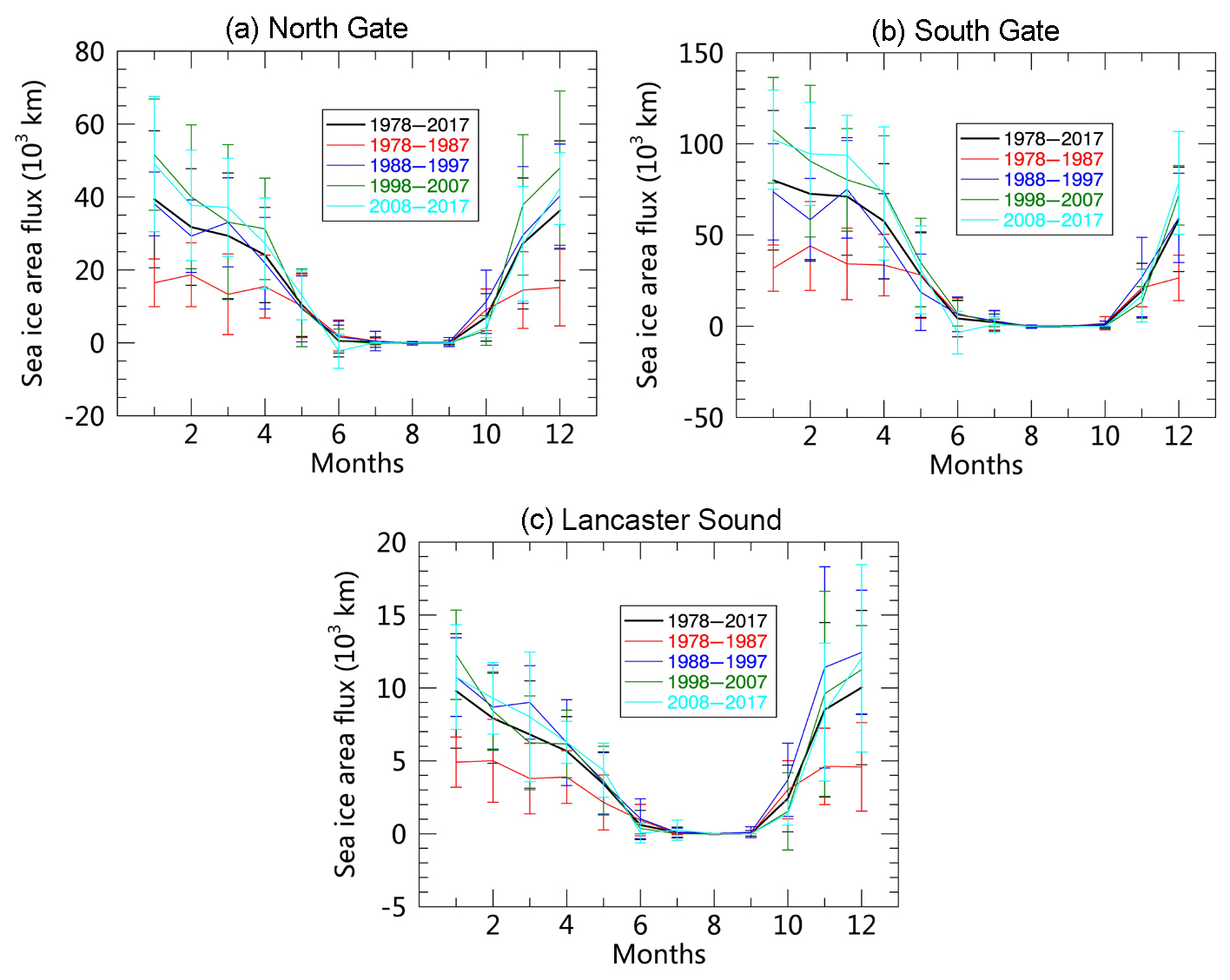
Figure 11Monthly mean sea ice area export in (a) the northern gate, (b) the southern gate, and (c) Lancaster Sound. Both the climatology (1978–1979 to 2016–2017) and decadal mean fields are given in the panels.
4.2 Variability and trends of seasonal and annual inflow and outflow
Figure 12 shows the seasonal and annual sea ice area flux across the three gates. The seasonally accumulative flux fields are obtained for the months of spring (March–May), summer (June–August), autumn (September–November), and winter (December–February). The annual sea ice flux refers to the sum of monthly flux from September to the following August.
Distinct interannual variation is evident in the annual sea ice flux fields as well as in the winter and spring fluxes (Fig. 12). Table 2 shows that the average annual inflow across the northern gate is 205.8 ( km2, with minimum annual inflow in 1980–1981 (64.1×10³ km2) and maximum annual inflow (414.8×10³ km2) in 2006–2007. The southern gate shows a mean annual outflow of 394.3 ( km2, with annual outflow ranging between 140.6×10³ km2 (1980–1981) and 727.4×10³ km2 (2008–2009). The mean annual inflow through Lancaster Sound is 55.2 ( km2, with outflow varying between 20.7×10³ km2 (1978–1979) and 94.3×10³ km2 (2014–2015). The difference between the inflow (through the northern gate and Lancaster Sound) and outflow (through the southern gate), km2, is suggestive of annual net loss of sea ice area in the regions between ∼65 and ∼75∘ N in Baffin Bay.
We obtain a total sea ice inflow of 214.7×10³ km2 during the cold seasons (winter and spring) through the northern gate and Lancaster Sound and an outflow of 368.0×10³ km2 via the southern gate. The difference of 153.3×10³ km2 is largely balanced by newly formed ice within the bay, revealing Baffin Bay itself as an important source regime of sea ice. Using km2 as the area of Baffin Bay, this newly formed ice within the bay represents a noteworthy fraction of 22.2 % of the coverage of Baffin Bay. As mentioned above, the sea ice motion fields in the bay gradually increase from north to south (Fig. 8a), resulting in a distinct ice speed gradient and possibly the occurrence of new leads (not shown). Therefore, the sea ice dynamics of the central and western regions of the bay are dominated by a sea ice diverging pattern (as exemplified in Fig. 13), where new ice can form from the freezing process in leads. For the warm period (summer and autumn), both sea ice inflow (46.3×10³ km2) and outflow (26.3×10³ km2) are small. The difference of km2 represents net sea ice loss that is likely due to enhanced melting in the bay. This finding emphasizes that Baffin Bay serves as an important ice sink area during the warm seasons.
Table 2Seasonal and annual mean sea ice area flux across different gates (103 km2).
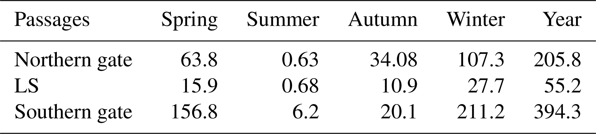
Note that spring is March–May, summer is June–August, autumn is September–November, winter is December–February, and a year is September–August.
Figure 12 shows that all three gates experienced significant positive trends in annual flux over the past four decades, with the major contributions originating from the flux increases during the cold seasons (winter and spring). The trend for the northern gate, approximately 38.9×10³ km2 decade−1 (or 19.0 % decade−1), is significant (Fig. 12a). The percentage trend denotes the fractional change relative to the climatological estimate of flux for 1978–1979 to 2016–2017. A larger annual increase of 82.2×10³ km2 decade−1 (or 21.1 % decade−1) is observed for the southern gate (Fig. 12b). The increase in ice flux through Lancaster Sound, 7.5×10³ km2 decade−1 (or 13.6 % decade−1), is small but significant (Fig. 12c). All these trend estimates have passed the 99 % confidence test. Therefore, the increased sea ice outflow across the southern gate has been partly compensated for by the enhanced inflows via the northern gate and Lancaster Sound. The increased outflow across this gate is also partially compensated for by the increased occurrence of new ice area formed within the bay.
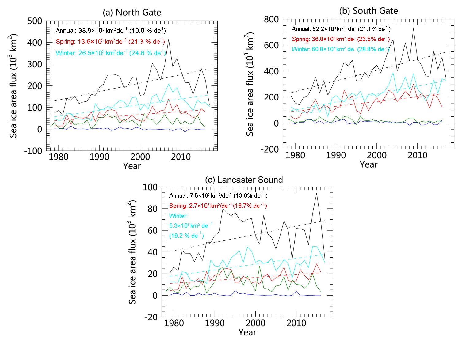
Figure 12Time series of annual (September–August) sea ice area flux (thick black line) across (a) the northern gate, (b) the southern gate, and (c) Lancaster Sound. Seasonal flux is estimated for winter (December–February, cyan line), spring (March–May, red line), summer (June–August, green line), and autumn (September–November, blue line). The dashed lines represent the linearly fitted trends. The annual and cold-season (winter and spring) trends are all significant at the 99 % level. However, for the warm seasons (summer and autumn), the trends are not statistically significant and are not shown in the panels.
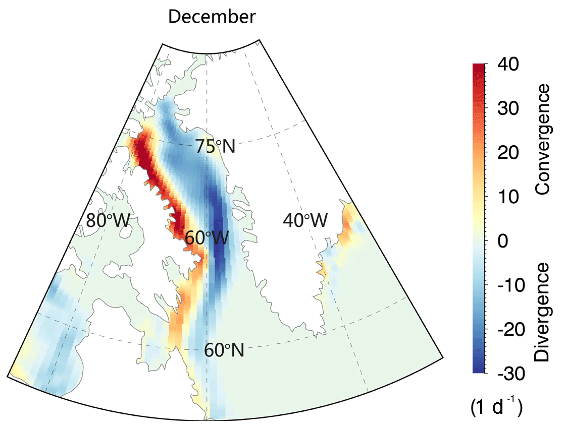
Figure 13Divergence and convergence fields derived from the climatological (1978–1979 to 2016–2017) sea ice motion vector fields in December using Eq. (3).
5.1 Possible sources of sea ice inflow into northern Baffin Bay
The sources that contribute to the ice area changes in the north of Baffin Bay, i.e., the area flux through the northern gate, include (1) inflow from the Arctic Ocean through Nares Strait, (2) inflow from the Canadian Arctic Archipelago (CAA) across Lancaster Sound and Jones Sound (JS), and (3) ice production in NOW in the bay.
5.1.1 Nares Strait sea ice inflow through Smith Sound
Sea ice transport in Nares Strait is controlled by the formation of ice bridges in Nares Strait. As reported based on RADARSAT SAR imagery by Kwok (2007), ice bridges form due to increases in the strength of ice arches in middle to late winter and collapse due to warm temperatures in early summer. Arching is commonly observed in Kane Basin at the southern end of Nares Strait and another occurs at the northern end. Over a 13-year period (1997–2009), the southern arch formed in all years except 2009, whereas half of the winters lacked the northern arch (Kwok, 2007). The formation of the southern arch may depend on upstream ice conditions, and the formation of the northern arch in the northern inlet of Nares Strait may be favored by the creation of the southern arch. The locations of the two ice arches are shown in Fig. S1a.
It is clear that when the southern arch forms, there exist conditions under which sea ice inflow through Nares Strait into Baffin Bay is strongly restricted. Seasonal stoppages of Nares Strait ice flux into Baffin Bay are associated with the formation of the southern arch. The immediately mitigating effects due to the formation of ice bridges are apparent from the cases in 2007. During that winter, no locations had conditions suitable for the formation of ice bridges, and area flux through Nares Strait reached a record high (87×103 km2). This large outflow accounted for 21.0 % of the annual ice flux (414.8×10³ km2) through the northern gate of Baffin Bay in 2006–2007.
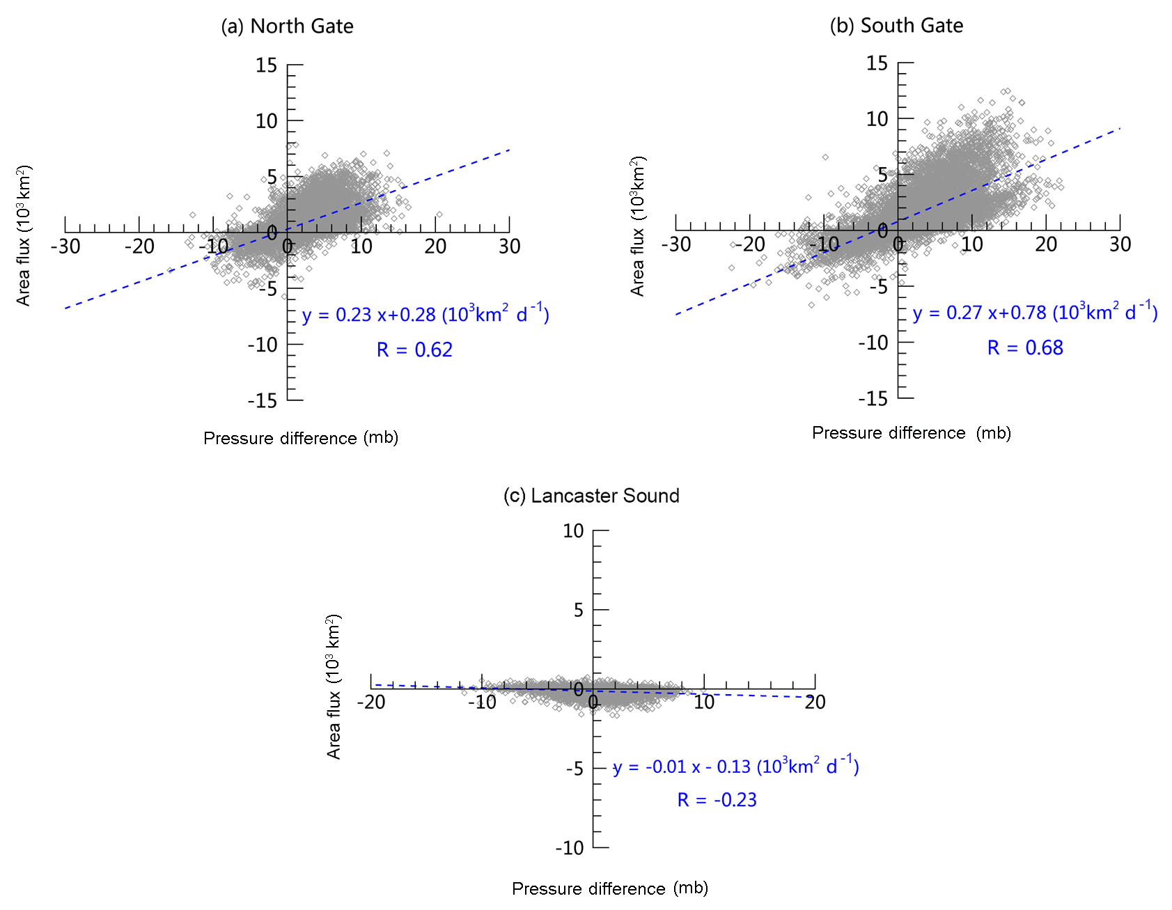
Figure 14Scatterplot of daily sea ice area flux and cross-gate pressure differences for (a) the northern gate, (b) the southern gate, and (c) Lancaster Sound.
Owing to the small width of Smith Sound (∼30 km), the sea ice area flux through Nares Strait cannot be accurately estimated using the coarse NSIDC drift data (25 km resolution), which may be subject to coastal contamination. With high-resolution SAR ice motion data (sampled on a 5 km grid), Kwok (2005) and Kwok et al. (2010) obtained Arctic sea ice inflow through Nares Strait. They estimated an average annual (September–August) ice area flux of 33×103 km2 for a 6-year period (1996–2002) and an annual average area flux of 42×103 km2 for a longer 13-year period (1996–2009). Therefore, sea ice area export via Nares Strait into the north of Baffin Bay between 1996–1997 and 2008–2009 may contribute a notable fraction (23.3 %) of the total ice area flux via the northern gate for the same period (280.2×10³ km2).
5.1.2 Sea ice inflow from the Canadian Arctic Archipelago
The sea ice exchange between the CAA and northern Baffin Bay was mainly through Lancaster Sound and the Jones Sound. However, sea ice inflow from the two sounds to Baffin Bay is difficult to quantify. In an early study for the 1970s, Dey (1981) roughly estimated the average annual inflows of 170×103 and 20×103 km2 for the Lancaster Sound and Jones Sound. The sea ice motion fields used were derived from diverse sources, including coarse satellite imagery and airborne observations measurements, as well as field measurements. Therefore, their estimates only correspond to a rough estimate.
In a recent study, Agnew et al. (2008) applied a spatially enhanced AMSR-E sea ice motion (13.5 km) to assess the sea ice area flux across CAA for the period from 2002–2003 to 2006–2007. During the 5-year period, sea ice is exported 68×103 km2 for each year across the Lancaster Sound into Baffin Bay. By contrast, the average sea ice inflow across Jones Sound approaches zero. The Lancaster Sound sea ice inflow is estimated to be 58.2×10³ km2 for the same period, which is comparable to the Agnew's results based on the AMSR-E imagery. Therefore, the Lancaster Sound constitutes one of the important ice sources for the sea ice into the north of Baffin Bay.
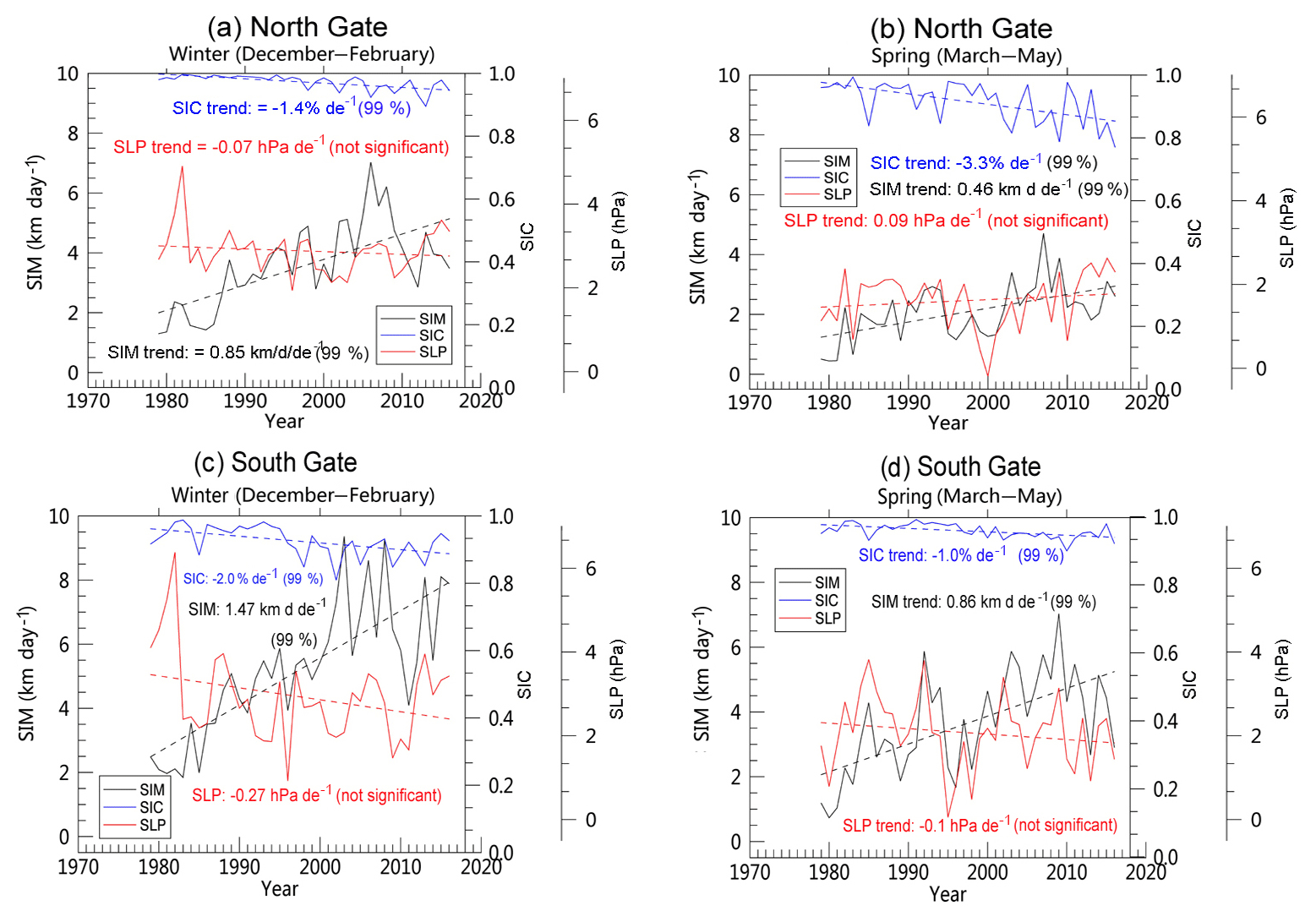
Figure 15Trends and variability of cross-gate mean sea ice motion (thick black line) and concentration (thick blue line) for the (a, b) northern gate and (c, d) southern gate. The linear fit line for each parameter is shown as a dashed line. Cross-gate sea level pressure (SLP) difference (red) is shown to facilitate the analysis of causes of the significant trends in sea ice motion.
5.1.3 Sea ice production in the North Water Polynya
The NOW is a distinct feature in northern Baffin Bay. As shown in Fig. 6, it usually occupies an area at the northern end of Baffin Bay (north of 75∘ N) and serves as a large ice production area during freezing periods. As mentioned above, its emergence is largely attributable to the formation of an ice bridge at the southern end of Nares Strait (Fig. S1a), which controls the sea ice inflow. Maintained by strong northerly winds and ocean currents, this large polynya is frequently exposed and so are new sea ice grows within it; this new ice is then transported southward. Based on previously reported CAA inflow through Smith Sound (42×103 km2) and Jones Sound (0–20×103 km2), we obtain a preliminary estimate of annual mean area production in the NOW (218–238×103 km2) for the period 1996–1997 to 2008–2009. To obtain this estimate, sea ice from the two inflow sources are subtracted from the mean annual ice flux of the northern gate (280.2×10³ km2) of the corresponding period. The results suggest the major part (approximately 78–85 %) of the sea ice entering via the northern gate is likely produced in the polynya.
5.2 Connections to cross-gate sea level pressure gradient
If free drift conditions are allowed, sea ice motion is mainly wind-driven and parallel to the sea level pressure isobars (Thorndike and Colony, 1982). In this study, the response of daily sea ice flux to the cross-gate pressure gradient was investigated. The gradient is defined as the difference in mean sea level pressure (SLP) between the eastern and western endpoints of each fluxgate. The positive (negative) gradient corresponds to positive (negative) sea ice flux. The data pairs of SLP gradient difference and ice area flux for each gate are shown in Fig. 14. Clearly, the cross-gate SLP difference is a good predictor of the variance of sea ice flux for the north (Fig. 14a) and southern gates (Fig. 14b), with correlations of 0.62 and 0.68. These correlations are statistically significant at the 99 % confidence level. The stronger slope in the southern gate (0.27) is suggestive of an ice condition that is thinner and perhaps closer to free drift than that of the northern gate (0.23). Lancaster Sound, however, reveals an overall counter gradient ice motion (), although it is not significant (Fig. 14c). Sea ice in this narrow channel is largely controlled by internal ice stresses caused by local sea ice interactions and orographic conditions. As a consequence, sea ice floes in the sound can not move as freely as those in the interior part of Baffin Bay.
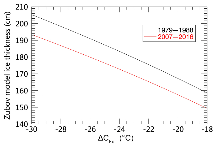
Figure 16Modeled sea ice thickness change as a function of freezing degree (daily average, ΔCFd) for early (1979–1987) and recent (2007–2016) decades.
5.3 Causes of the enhanced sea ice area flux
5.3.1 Potential contribution of geostrophic winds?
According to Eq. (1), sea ice motion and concentration are the two essential input parameters used to estimate area flux. Potentially, their changes would be reflected in the variations of flux. Figure 15 depicts the interannual variations and trends of the two relevant sea ice parameters for the cold seasons (winter and summer) at the northern and southern gates. As mentioned above and shown in Fig. 12, all three fluxgates show significant increases in sea ice area flux during the cold seasons. This is mainly caused by the increasing trend in sea ice motion (Fig. 15). On the other hand, the decreasing trend in sea ice concentration may have contributed negatively to ice area flux. The trends are all significant at the 99 % level. The increasing or decreasing trends of different parameters at each fluxgate in the context of the entire bay are illustrated in Figs. 9 and 10.
Figure 15 displays the records of cross-gate SLP difference (thick red line), a proxy for the strength of geostropic winds. Although the SLP difference is a good predictor of the interannual variability in ice motion (see Sect. 5.2 for more details), it does not show any significant trend over the nearly 40-year period. This observation eliminates wind force as a main driver of the positive trends in ice motion and area flux fields.
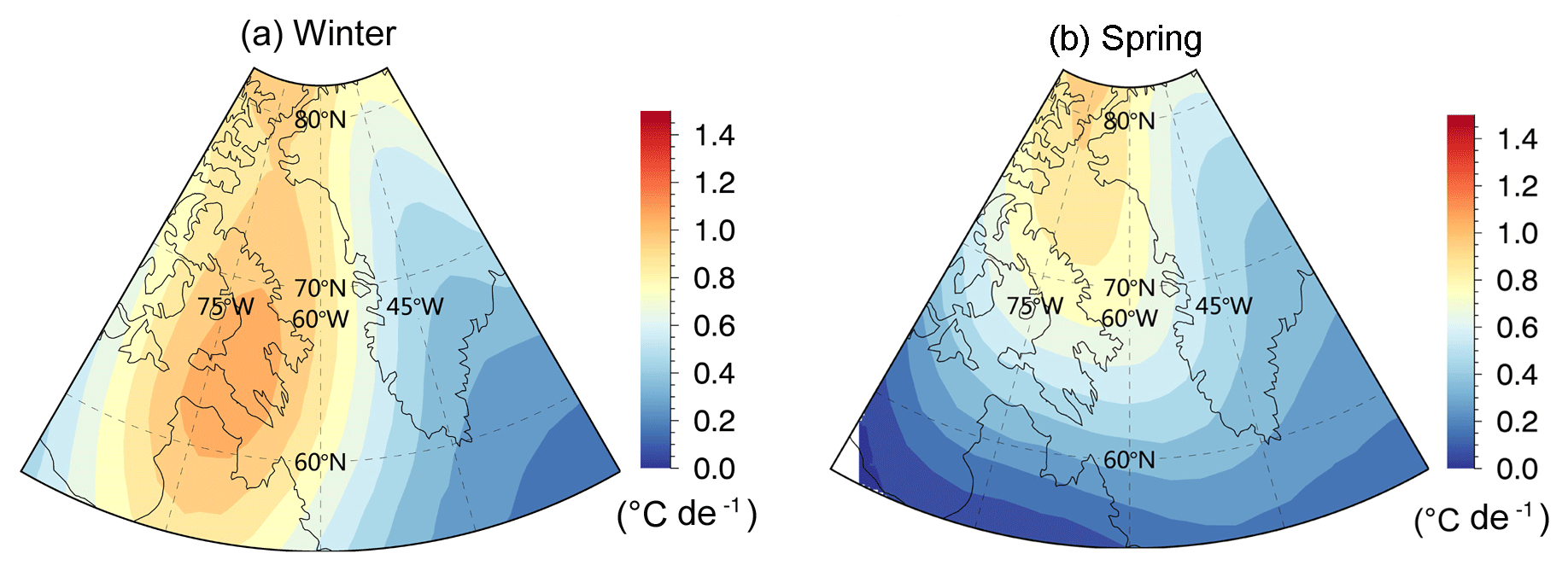
Figure 17Surface air temperature trends for the period 1978–1979 to 2016–2017 during (a) winter and (b) spring.
5.3.2 Changes in sea ice
Here we examine the changes in sea ice itself, specifically (1) the changes in sea ice concentration and (2) the changes in sea ice thickness. A reduced sea ice concentration is expected to cause a decreased area flux across the fluxgates. On the other hand, it implies a less compacted ice pack and facilitates sea ice drift and, perhaps, an increase in area flux. Despite the decline in sea ice concentration at each gate during the cold periods, the sea ice generally remains at a compact level above 90 % (Fig. 15), at which large ice internal ice stress is still expected. Therefore, sea ice concentration changes cannot be a primary driver of the enhanced ice motion and area flux.
Due to the scarcity of direct ice thickness measurements, we obtain an approximation of ice thickness changes with time following the Zubov ice growth model. The associated cumulative freezing degree (CFd) is derived from surface air temperatures. This variable is directly related to the level of sea ice growth. Modeled ice thickness fields for different periods are shown in Fig. 16 as a function of ΔCFd, where ΔCFd denotes the average daily freezing degree (∘C) of the whole growth period. That is, , where Fd is the total days of an ice growth period.
The downward slope of each line in Fig. 16 (−3.83 and −3.75 cm ∘C−1 for early and recent decades) represents the changes in thickness with freezing air temperature. There is an increasing trend in SAT in the bay of 0.95 ∘C decade−1 (Fig. 17). Based on estimates displayed in Fig. 16, this air temperature enhancement implies a SAT increase in the bay of 3.8 ∘C in the recent decade, which can be expected to cause thickness declines of 14.6 cm and 14.3 cm (i.e., multiplying slope by 3.8 ∘C) for the early and recent decades.
The systematic bias between the two lines in Fig. 16, one for each decade, corresponds to the ice thickness change in association with the change in the length of the freezing period. Due to warmer surface air in the recent decade, a difference in ice growth period of approximately 20 days is observed between the two decades (i.e., approximately −5 days decade−1), which is consistent with the delayed freezing and earlier melting dates in Baffin Bay (Stroeve et al., 2014). When taking into account the freezing period changes, a further ∼10 cm decline is identified due to the shortened days of freezing (Fig. 11). Therefore, the increased SAT, together with the shortened length of the ice-freezing period, can be expected to cause an average reduction in sea ice thickness of 24.6 cm.
According to Eq. (2), sea ice motion acceleration due to air and current dragging force (τa and τw) is proportional to the inversion of thickness change (i.e., 1 h). Therefore, the recent ice thickness decline of 24.6 cm for ice with a typical thickness of 1.8 m would lead to enhanced ice motion, 1.16 times that of the early decade. A recent study indicates that air–ice (water–ice) drag coefficient in Baffin Bay could have a trend of approximately of yr−1 ( yr−1) (Tsamados et al., 2014). Taking into account these trends, an air (water) dragging force would have accelerated the sea ice motion by approximately 1.27 (1.48) times. Now, recent sea ice speed can be enhanced by 1.47–1.72 times in comparison with that in the earlier period, when thicker ice and small drag coefficients prevailed.
Although the ice growth model used here is simple, it can reflect the basic trend in declining ice thickness over past decades. As indicated by the field measurements (Kurtz and Farrell, 2011), recent snow depth over first-year ice in the Arctic Ocean seems to be reduced by a half. Another study suggests that decreased snow depth and ice thickness will increase the sea ice thickness growth rate and delay (but not reverse) the sea ice thickness decline trend (https://www.sciencedaily.com/releases/2018/12/181206114700.htm, last access: 1 February 2019). Therefore, using Eq. (2) to estimate sea ice thickness changes without considering the effects of snow changes may overestimate the declining trend in sea ice thickness. However, our estimates suggest that winter and spring sea ice motion in Baffin Bay in the recent decade are on average 1.6 times greater than those in the early decade. This is comparable in magnitude to the ice motion changes (our calculations) that are dependent on the changes with respect to decreased thickness and increased drag coefficients. To summarize this section, the sea ice motion and area flux increases in Baffin Bay over the past four decades are mainly attributable to a thinner sea ice thickness, which is primarily associated with the increase in surface air temperature. This is consistent with findings in the Arctic Ocean (Rampal et al., 2009; Spreen et al., 2011; Kwok et al., 2013). Also, air and water drag coefficient changes also contribute an significant part to the sea ice motion increases.
With satellite-derived sea ice parameters, we estimated the sea ice inflow and outflow through the key fluxgates of Baffin Bay. The record of sea ice area flux was extended to span a nearly 40-year period from 1978–1979 to 2016–2017. On the basis of the estimates, the variability and trends of sea ice area flux through the three fluxgates are examined in detail (northern gate, Lancaster Sound, and southern gate) for different timescales (monthly, seasonal, and annual flux). Large interannual variations are detected for the different flux fields. Moreover, significant increasing trends are identified for the annual ice flux for the three gates, with the primary contributions from those during winter (December–February) and spring (March–May).
The spatiotemporal differences are obvious for the sea ice flux through different gates. On average, there is an inflow through the northern gate (205.8×10³ km2) and Lancaster Sound (55.2×10³ km2) and an outflow via the southern gate (394.3×10³ km2). During cold seasons (winter and spring), the difference between inflow and outflow (i.e., inflow minus outflow) amounts to km2 and is largely replenished by new ice formed within the bay that is likely associated with the divergence mechanism. For the warm period (summer and autumn), the sea ice inflows (46.3×10³ km2) and outflows (26.3×10³ km2) are small, pointing to a net ice area loss of 20.0×10³ km2 that is connected to melting processes in the bay. This emphasizes that Baffin Bay serves as not only as an area of ice source during cold periods but also as an area of ice sink during warm periods. The sea ice growth and melting processes could influence the ocean current properties in Baffin Bay. With regard to the diverse ice inflow sources into the north of Baffin Bay through the northern gate, the comparisons with published results seem to tally well with the fact that the majority (about 75 %–85 %) of the ice area originates from ice growth in NOW, in addition to the ice inputs via Nares Strait, Lancaster Sound, and Jones Sound.
The interannual variability of ice flux across the northern and southern gates is in part linked to wind forcing associated with the cross-gate SLP differences, while the ice flow through Lancaster Sound is largely determined by orographic conditions. The trends for the three gates (northern gate: 38.9×10³ km2 decade−1; southern gate: 82.2×10³ km2 decade−1; Lancaster Sound: 7.5×10³ km2 decade−1) are significant and are primarily explained by the increasing ice motion and to a small fraction by the decreasing ice concentration. The preliminary simulation demonstrates that the sea ice motion, which has been accelerated over the past four decades, is mainly attributable to the decline in ice thickness and the increase in the air and water drag coefficients in Baffin Bay. Furthermore, modeling results unveiled that the warmer climate plays a decisive role in generating thinner ice in the bay.
Sea ice motion data are available at http://nsidc.org/data/NSIDC-0116 (Tschudi et al., 2019). IABP sea ice drift data used to assess the NSIDC product are available at http://iabp.apl.washington.edu/ (last access: 20 March 2019). Sea ice concentration data employed to calculate sea ice area flux are available at http://nsidc.org/data/NSIDC-0079 (Comiso, 2017). The CIS map used to analyze the sea ice conditions in Baffin Bay is available at https://www.canada.ca/en/environment-climate-change/services/iceforecasts-observations/latest-conditions.html. The reanalysis data of SLP and SAT are available at https://www.esrl.noaa.gov/psd/cgi-bin/db_search/DBListFiles.pl?did=195&tid=72450&vid=676 (last access: 20 December 2018) and https://www.esrl.noaa.gov/psd/cgi-bin/db_search/DBListFiles.pl?did=195&tid=72451&vid=3083 (last access: 20 March 2018).
The supplement related to this article is available online at: https://doi.org/10.5194/tc-13-1025-2019-supplement.
HB led the analysis and integrated the data. ZZ, YW, XX, YL, and JH processed the sea ice motion data. YL and MF performed the area flux calculations. HB, ZZ, and YW drafted the paper. All authors discussed the results and commented on the paper.
The authors declare that they have no conflict of interest.
The authors would like to thank the data providers as follows. NSIDC provided the satellite-derived ice motion and concentration data, and National Centers for Environmental Prediction/National Center for Atmospheric Research (NCEP/NCAR) provided the reanalysis product. We are grateful for the suggestions from Jinlun, Zhang, Mike Steel, Axel Schweiger (University of Washington). Also, we appreciate the constructive comments from the three anonymous reviewers. This work was supported by the National Natural Science Foundation of China under grants 41406215 and 41706194, a fund provided by the Qingdao National Laboratory for Marine Science and Technology, and the NSFC-Shandong Joint Fund for Marine Science Research Centers (U1606401).
This paper was edited by John Yackel and reviewed by three anonymous referees.
Aagaard, K. and Carmack, E. C.: The role of sea ice and other fresh water in the Arctic circulation, J. Geophys. Res.-Oceans, 94, 14485–14498, 1989.
Agnew, T., Lambe, A., and Long, D.: Estimating sea ice area flux across the Canadian Arctic Archipelago using enhanced AMSR-E, J. Geophys. Res., 113, C10011, https://doi.org/10.1029/2007JC004582, 2008.
Bi, H., Huang, H., Fu, M., Fu, T., Zhou, X., and Xu, X.: Estimating sea-ice volume flux out of the Laptev Sea using multiple satellite observations, Polar Res., 35, 1–13, https://doi.org/10.3402/polar.v35.24875, 2016a.
Bi, H., Sun, K., Zhou, X., Huang, H., and Xu, X.: Arctic Sea Ice Area Export Through the Fram Strait Estimated From Satellite-Based Data:1988–2012, IEEE J. Select. Top. Appl. Earth Observ. Remote Sens., 9, 3144–3157, 2016b.
Cho, K., Sasaki, N., Shimoda, H., Sakata, T., and Nishio, F.: Evaluation and improvement of SSM/I sea ice concentration algorithms for the Sea of Okhotsk, J. Remote Sens. Soc. JPN, 16, 47–58, 1996.
Cimatoribus, A. A., Drijfhout, S. S., Toom, M. D., and Dijkstra, H. A.: Sensitivity of the Atlantic meridional overturning circulation to South Atlantic freshwater anomalies, Clim. Dynam., 39, 2291–2306, 2012.
Comiso, J. C.: Bootstrap Sea Ice Concentrations from Nimbus-7 SMMR and DMSP SSM/I-SSMIS, Version 3, Boulder, Colorado USA, NASA National Snow and Ice Data Center Distributed Active Archive Center, https://doi.org/10.5067/7Q8HCCWS4I0R, 2017.
Comiso, J. C., Gersten, R., Stock, L., Turner, J., Perez, G., and Cho, K.: Positive trends in the Antarctic sea ice cover and associated changes in surface temperature, J. Climate, 30, 2251–2267, https://doi.org/10.1175/JCLI-D-0408.1, 2017a.
Comiso, J. C., Meier, W. N., and Gersten, R.: Variability and trends in the Arctic Sea ice cover: Results from different techniques, J. Geophys. Res., 122, 6883–6900, https://doi.org/10.1002/2017JC012768, 2017b.
Cuny, J., Rhines, P. B., and Kwok, R.: Davis Strait volume, freshwater and heat fluxes, Deep Sea Res. Part I, 52, 519–542, 2005.
Cuny, J., Rhines, P. B., and Niiler, P. P.: Labrador Sea Boundary Currents and the Fate of the Irminger Sea Water, J. Phys. Oceanogr., 32, 627–647, 2002.
Curry, B., Lee, C. M., Moritz, R. E., and Kwok, R.: Multiyear Volume, Liquid Freshwater, and Sea Ice Transports through Davis Strait, 2004-10, J. Phys. Oceanogr., 44, 1244–1266, 2014.
Dey, B.: Monitoring winter sea ice dynamics in the Canadian Acctic with NOAA-TIR images, J. Geophys. Res.-Oceans, 86, 3223–3235, 1981.
Dunlap, E. and Tang, C. L.: Modelling the mean circulation of Baffin Bay, Atmosphere, 44, 99–109, 2006.
Goosse, H., Fichefet, T., and Campin, J. M.: The effects of the water flow through the Canadian Archipelago in a global ice-ocean model, Geophys. Res. Lett., 24, 1507–1510, 1997.
Graham, R. M., Cohen, L., Petty, A. A., Boisvert, L. N., Rinke, A., Hudson, S. R., Nicolaus, M., and Granskog, M. A.: Increasing frequency and duration of Arctic winter warming events, Geophys. Res. Lett., 44, 6974–6983, 2017.
Hawkins, E., Smith, R. S., Allison, L. C., Gregory, J. M., Woollings, T. J., Pohlmann, H., and Cuevas, B. D.: Bistability of the Atlantic overturning circulation in a global climate model and links to ocean freshwater transport, Geophys. Res. Lett., 38, 415–421, 2011.
Holland, M. M., Bitz, C. M., Eby, M., and Weaver, A. J.: The Role of Ice-Ocean Interactions in the Variability of the North Atlantic Thermohaline Circulation, J. Climate, 14, 656–675, 2001.
Jahn, A., Tremblay, B., Mysak, L. A., and Newton, R.: Effect of the large-scale atmospheric circulation on the variability of the Arctic Ocean freshwater export, Clim. Dynam., 34, 201–222, 2010.
Kalnay, E., Kanamitsu, M., Kistler, R., Collins, W., Deaven, D., Gandin, L., Iredell, M., Saha, S., White, G., and Woollen, J.: The NCEP/NCAR 40-Year Reanalysis Project, B. Am. Meteorol. Soc., 77, 437–472, 1996.
Kurtz, N. T and Farrell, S. L.: Large-scale surveys of snow depth on Arctic sea ice from Operation IceBridge, Geophys. Res. Lett., 38, L20505, https://doi.org/10.1029/2011GL049216, 2011.
Krumpen, T., Janout, M., Hodges, K. I., Gerdes, R., Girard-Ardhuin, F., Hölemann, J. A., and Willmes, S.: Variability and trends in Laptev Sea ice outflow between 1992–2011, The Cryosphere, 7, 349–363, https://doi.org/10.5194/tc-7-349-2013, 2013.
Krumpen, T., Gerdes, R., Haas, C., Hendricks, S., Herber, A., Selyuzhenok, V., Smedsrud, L., and Spreen, G.: Recent summer sea ice thickness surveys in Fram Strait and associated ice volume fluxes, The Cryosphere, 10, 523–534, https://doi.org/10.5194/tc-10-523-2016, 2016.
Kwok, R., Curlander, J. C., and Pang, S. S.: An ice-motion tracking system at the Alaska SAR facility, IEEE J. Ocean. Eng., 15, 44–54, 1990.
Kwok, R.: Variability of Nares Strait ice flux, Geophys. Res. Lett., 32, 1064–1067, 2005.
Kwok, R.: Baffin Bay ice drift and export: 2002–2007, Geophys. Res. Lett., 34, 2002–2007, 2007.
Kwok, R.: Outflow of Arctic ocean sea ice into the Greenland and Barents Seas: 1979–2007, J. Climate, 22, 2438–2457, 2009.
Kwok, R., Maslowski, W., and Laxon, S. W.: On large outflows of Arctic sea ice into the Barents Sea, Geophys. Res. Lett., 32, 45–81, 2005.
Kwok, R., Toudal, P. L., Gudmsen, P., and Pang, S. S.: Large sea ice outflow into the Nares Strait in 2007, Geophys. Res. Lett., 37, 93–101, 2010.
Kwok, R., Spreen, G., and Pang, S.: Arctic sea ice circulation and drift speed: Decadal trends and ocean currents, J. Geophys. Res.-Oceans, 118, 2408–2425, 2013.
Melling, H., Gratton, Y., and Ingram, G.: Ocean circulation within the North Water polynya of Baffin Bay, Atmosphere, 39, 301–325, 2001.
Parkinson, C. L. and Cavalieri, D. J.: A 21 year record of Arctic sea-ice extents and their regional, seasonal and monthly variability and trends, Ann. Glaciol., 34, 441–446, 2017.
Peterson, I. K. and Pettipas, R.: Trends In air temperature and sea ice in the Atlantic Large Aquatic Basin and adjoining areas, Canadian Technical Report, Hydrography, Ocean Science, 290, 3–8, 2013.
Rampal, P., Weiss, J., and Marsan, D.: Positive trend in the mean speed and deformation rate of Arctic sea ice, 1979–2007, J. Geophys. Res.-Oceans, 114, C05013, https://doi.org/10.1029/2008JC005066, 2009.
Rudels, B.: The outflow of polar water through the Arctic Archipelago and the oceanographic conditions in Baffin Bay, Pol. Res., 4, 161–180, 2010.
Serreze, M. C., Barrett, A. P., Stroeve, J. C., Kindig, D. N., and Holland, M. M.: The emergence of surface-based Arctic amplification, The Cryosphere, 3, 11–19, https://doi.org/10.5194/tc-3-11-2009, 2009.
Smedsrud, L. H., Sirevaag, A., Kloster, K., Sorteberg, A., and Sandven, S.: Recent wind driven high sea ice area export in the Fram Strait contributes to Arctic sea ice decline, The Cryosphere, 5, 821–829, https://doi.org/10.5194/tc-5-821-2011, 2011.
Smedsrud, L. H., Halvorsen, M. H., Stroeve, J. C., Zhang, R., and Kloster, K.: Fram Strait sea ice export variability and September Arctic sea ice extent over the last 80 years, The Cryosphere, 11, 65–79, https://doi.org/10.5194/tc-11-65-2017, 2017.
Spreen, G., Kern, S., Stammer, D., Forsberg, R., and Haarpaintner, J.: Satellite-based estimates of sea-ice volume flux through Fram Strait, Ann. Glaciol., 44, 321–328, 2006.
Spreen, G., Kwok, R., and Menemenlis, D.: Trends in Arctic sea ice drift and role of wind forcing: 1992–2009, Geophys. Res. Lett., 38, L19501, https://doi.org/10.1029/2011GL048970, 2011.
Stern, H. L. and Heide-Jørgensen, M. P.: Trends and variability of sea ice in Baffin Bay and Davis Strait, 1953–2001, Pol. Res., 22, 11–18, 2003.
Stroeve, J. C., Markus, T., Boisvert, L., Miller, J., and Barrett, A.: Changes in Arctic melt season and implications for sea ice loss, Geophys. Res. Lett., 41, 1216–1225, 2014.
Stroeve, J. C., Schroder, D., Tsamados, M., and Feltham, D.: Warm winter, thin ice?, The Cryosphere, 12, 1791–1809, https://doi.org/10.5194/tc-12-1791-2018, 2018.
Sumata, H., Gerdes, R., Kauker, F., and Karcher, M.: Empirical error functions for monthly mean Arctic sea-ice drift, J. Geophys. Res., 120, 7450–7475, 2015.
Thorndike, A. S. and Colony, R.: Sea ice motion in response to geostrophic winds, J. Geophys. Res., 87, 5845–5852, 1982.
Tsamados, M., Feltham, D. L., Schroeder, D., Farrell, S. L., Krutz, N. T., Laxon, S. W., and Flocco, D.: Impact of Variable Atmospheric and Oceanic Form Drag on Simulations of Arctic Sea Ice, J. Phys. Oceanogr., 44, 1329–1353, 2014.
Tschudi, M., Fowler, C., Maslanik, J., Stewart, J. S., and Meier, W.: Polar Pathfinder Daily 25 km EASE-Grid Sea Ice Motion Vectors, Version 3, NSIDC, Boulder, Colorador, https://doi.org/10.5067/O57VAIT2AYYY, 2016.
Tschudi, M., Meier, W. N., Stewart, J. S., Fowler, C., and Maslanik, J.: Polar Pathfinder Daily 25 km EASE-Grid Sea Ice Motion Vectors, Version 4, Boulder, Colorado USA, NASA National Snow and Ice Data Center Distributed Active Archive Center, https://doi.org/10.5067/INAWUWO7QH7B, 2019.
Yang, Q., Dixon, T. H., Myers, P. G., Bonin, J., Chambers, D., van den Broeke, M. R., Ribergaard, M. H., and Mortensen, J.: Recent increases in Arctic freshwater flux affects Labrador Sea convection and Atlantic overturning circulation, Nat. Commun., 7, 10525, https://doi.org/10.1038/ncomms10525, 2016.
Zhang, Z., Bi, H., Huang, H., Liu, Y., and Yan, L.: Arctic sea ice volume export through the Fram Strait from combined satellite and model data: 1979–2012, Acta Oceanol. Sin., 36, 44–55, 2017.