the Creative Commons Attribution 4.0 License.
the Creative Commons Attribution 4.0 License.
 | 10 Jan 2018
Using satellite laser ranging to measure ice mass change in Greenland and Antarctica
Don P. Chambers
Minkang Cheng
A least squares inversion of satellite laser ranging (SLR) data over Greenland and Antarctica could extend gravimetry-based estimates of mass loss back to the early 1990s and fill any future gap between the current Gravity Recovery and Climate Experiment (GRACE) and the future GRACE Follow-On mission. The results of a simulation suggest that, while separating the mass change between Greenland and Antarctica is not possible at the limited spatial resolution of the SLR data, estimating the total combined mass change of the two areas is feasible. When the method is applied to real SLR and GRACE gravity series, we find significantly different estimates of inverted mass loss. There are large, unpredictable, interannual differences between the two inverted data types, making us conclude that the current 5×5 spherical harmonic SLR series cannot be used to stand in for GRACE. However, a comparison with the longer IMBIE time series suggests that on a 20-year time frame, the inverted SLR series' interannual excursions may average out, and the long-term mass loss estimate may be reasonable.
- Article
(3362 KB) - Full-text XML
-
Supplement
(2940 KB) - BibTeX
- EndNote


Since the Gravity Recovery and Climate Experiment (GRACE) was launched in 2002 (Tapley et al., 2004), it has provided an excellent time series of mass change integrated over Greenland and Antarctica's ice sheets (Jacob et al., 2012; Luthcke et al., 2013; Schrama and Wouters, 2011; Shepherd et al., 2012; Velicogna and Wahr, 2013). However, GRACE data go back to just mid-2002, and only a few other data series exist before then to study longer-term mass change. These include satellite altimetry (Howat et al., 2008; Johannessen et al., 2005; Shepherd et al., 2012) and the input–output method's combination of surface mass balance models and glacier flow speeds from interferometry (Rignot et al., 2011; Sasgen et al., 2012; Shepherd et al., 2012). Due to the paucity of data and their limited resolution in both space and time, estimates of ice mass change before GRACE are necessarily more uncertain. A high-quality satellite laser ranging (SLR) tracking data set (Cheng et al., 2011, 2013) for geodetic satellites is one possible additional data set that could be exploited to compute variability in ice mass before 2002, as it has existed for over a decade before GRACE.
Although SLR tracking data can be used to infer time-variable mass change (e.g., Nerem et al., 2000), it can only do so over a much longer wavelength. The resolution of SLR-based gravity fields is 8000 km at the equator (based on 5×5 spherical harmonic Stokes coefficients or a maximum degree/order of 5) compared to 660 km for GRACE (based on 60×60 spherical harmonics or a maximum degree/order of 60). This difference in resolution has resulted in few ice mass studies having been completed with SLR data. For example, Nerem and Wahr (2011) compared an SLR C20 Stokes coefficient time series with a time series from GRACE-based estimates of Greenland and Antarctica mass loss. This led them to suggest that the two ice sheets could explain the increase in the rate of change of C20 in the late 1990s. However, this analysis is not the same as our goals, as it used GRACE observations to explain SLR signals rather than determining mass change directly from the SLR data. More recently, Matsuo et al. (2013) used a 4×4 SLR-based gravity series to demonstrate the similarities between SLR and GRACE data in a general sense. They noted a similar mass loss over the entire Arctic and showed that the center of that mass loss occurred over roughly the same spatial extent. These two examples are promising and suggest that SLR and GRACE may be seeing comparable signals. However, as Matsuo et al. acknowledged, the low spatial resolution of the SLR data makes it “not feasible to obtain definitive estimates of the total amount of the mass change… even for an area as “large” as Greenland.”
To better resolve the SLR signal and obtain a more definitive estimate than Matsuo et al.'s direct method, we will utilize a least squares inversion technique to localize the SLR signal over Greenland and Antarctica. This technique provides us with time series of interannual variability as well as decadal-scale trends and accelerations over Greenland and Antarctica. We have two ultimate goals in this. First, to extend the time series of polar mass change backwards in time, before GRACE. And second, to serve as a gap-filler between GRACE and the future GRACE Follow-On mission. The original GRACE mission's last month of data was June of 2017, after several years of slowly degrading data quality and increasing gaps between monthly solutions. The Follow-On mission will not launch until at least March of 2018, leaving perhaps a year's gap in which no science data can be collected. Having a trusted gap-filling series which could also verify the quality of the later-mission GRACE data would be of benefit.
Data and methods are described in Sects. 2 and 3, and in the Supplement. In Sect. 4, we compare inversions of the SLR and GRACE data over Greenland and Antarctica during GRACE's 2003–2014 time frame and compare their trends and interannual signals. The implications of the results of our experiments, as well as the extension of the SLR data back to 1994, are discussed in Sect. 5.
The primary data series used here are a set of maximum degree/order 60 (60×60) monthly averaged spherical harmonic Stokes coefficients from GRACE (dates: 2003–2016) and a set of 5×5 monthly averaged spherical harmonic coefficients from SLR to a series of geodetic satellites (dates: 1994–2016). A second, more limited, set of 10×10 SLR coefficients is also tested for comparison (dates: 2000–2014).
The GRACE series used here is the standard CSR Release-05 spherical harmonic version (ftp://podaac.jpl.nasa.gov/allData/grace/L2/CSR/RL05/) (Bettadpur, 2012), with no constraints applied during processing. We apply the following standard post-processing steps: (1) C20 is replaced with the estimate derived from SLR tracking (ftp://podaac.jpl.nasa.gov/allData/grace/docs/TN-07_C20_SLR.txt) due to GRACE's known weakness in resolving that harmonic (Chambers, 2006), (2) a pole-tide correction is applied to harmonics C21 and S21 (Wahr et al., 2015), and (3) a GIA (global isostatic adjustment) model is removed. The GIA model is composed of the W12a GIA model (Whitehouse et al., 2012) south of 62∘ S, and the A et al. (2013) model north of 52∘ S, using a smoothed combination of the two between 52 and 62∘ S. No smoothing or destriping (e.g., Swenson et al., 2006; Chambers and Bonin, 2012) is applied, nor are any geocenter (degree 1) coefficients utilized. In addition to using the full 60×60 GRACE coefficients for 2003–2014, we also truncate down to 5×5 and 10×10 subsets to compare them more directly to the SLR data.
The primary SLR series used here (Cheng, 2017; Cheng et al., 2011, 2013) is a variant of the weekly, 5×5 SLR product created at the University of Texas Center for Space Research (CSR) and released alongside the GRACE series ftp://podaac.jpl.nasa.gov/allData/tellus/preview/L2/deg_5/CSR.Weekly.5x5.Gravity_Harmonics.txt). We use a version that is averaged monthly, rather than weekly, to make it more directly comparable to the monthly GRACE data. This version contains an estimate of C61∕S61 (but no other degree-6 harmonics) to avoid skewing the C21 harmonic due to a lack of sufficient degrees of freedom during the creation of the SLR gravity product (Cheng and Ries, 2017). The same GIA model is removed as with GRACE. Though the Cheng 5×5 SLR series exists from 1993 onwards, prior to November 1993, only four satellites were used in its creation (Starlette, Ajisai, and Lageos 1 and 2), whereas after that point, Stella was added as well. Because this change in satellite geometry could create possible jumps in the time series, we have only used data from 1994 onwards. The geocenter (degree 1) SLR terms are removed, both for the sake of comparison (because GRACE cannot perceive them) and because the SLR C10 term is suspected to have an incorrect trend caused by nonuniform ground network coverage (Collilieux et al., 2009; Wu et al., 2012). The geocenter terms commonly added to GRACE (Swenson et al., 2008) are expected to be more accurate, but they cannot be created for months in which GRACE does not exist and thus cannot be used at all before 2002. We found that using no geocenter at all brought our results closer to the results using GRACE-derived geocenter terms than using the original SLR geocenter terms did.
A pair of secondary SLR series (Sośnica et al., 2015), created at the Astronomical Institute at the University of Bern, are also considered for comparison, though they do not extend as far back in time as GRACE. Like the primary Cheng 5×5 SLR series, the two Sośnica SLR series were created from the combination of multiple-satellite SLR tracking data – mostly the five used in the Cheng 5×5 series but also including BLITS, Larets, Beacon-C, and LARES, over the time spans in which they exist. These series exist over the years 2000–2014 at monthly resolution. Two versions exist: an unconstrained case to a maximum degree/order of 6×6, and a constrained case to 10×10. Again, the geocenter terms are not included and the same GIA correction used in the GRACE processing is removed.
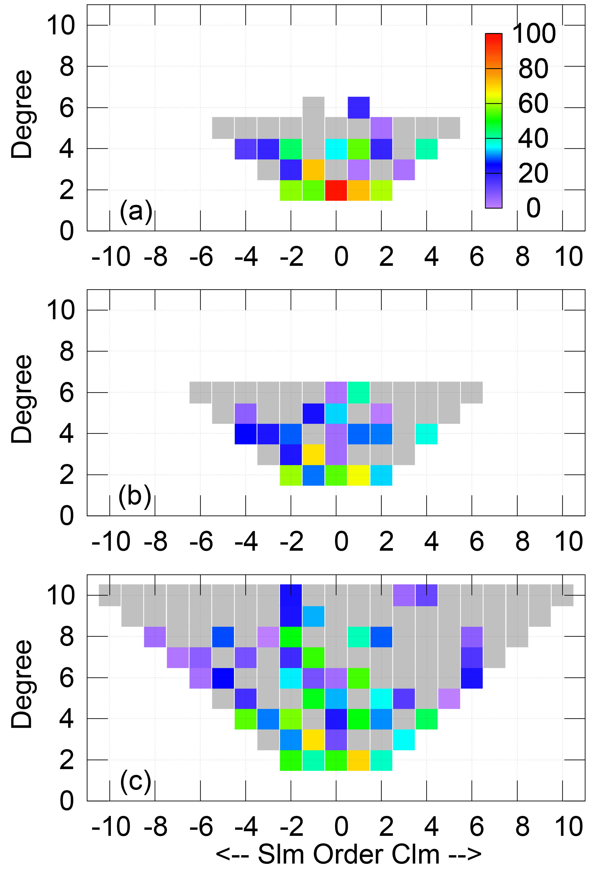
Figure 1Percent of GRACE variance explained by three SLR time series, after a 200-day smoother has been applied. SLR series are (a) Cheng et al's 5×5 series, (b) Sośnica et al's 6×6 unconstrained series, and (c) Sośnica et al's 10×10 constrained series. Harmonics with negative percent variance explain are shaded in grey. The C20 term in (a) is a perfect 1.0, because the GRACE C20 has been replaced by the SLR value. S harmonics are denoted as negative orders along the x axis, while C terms are listed as positive ones.
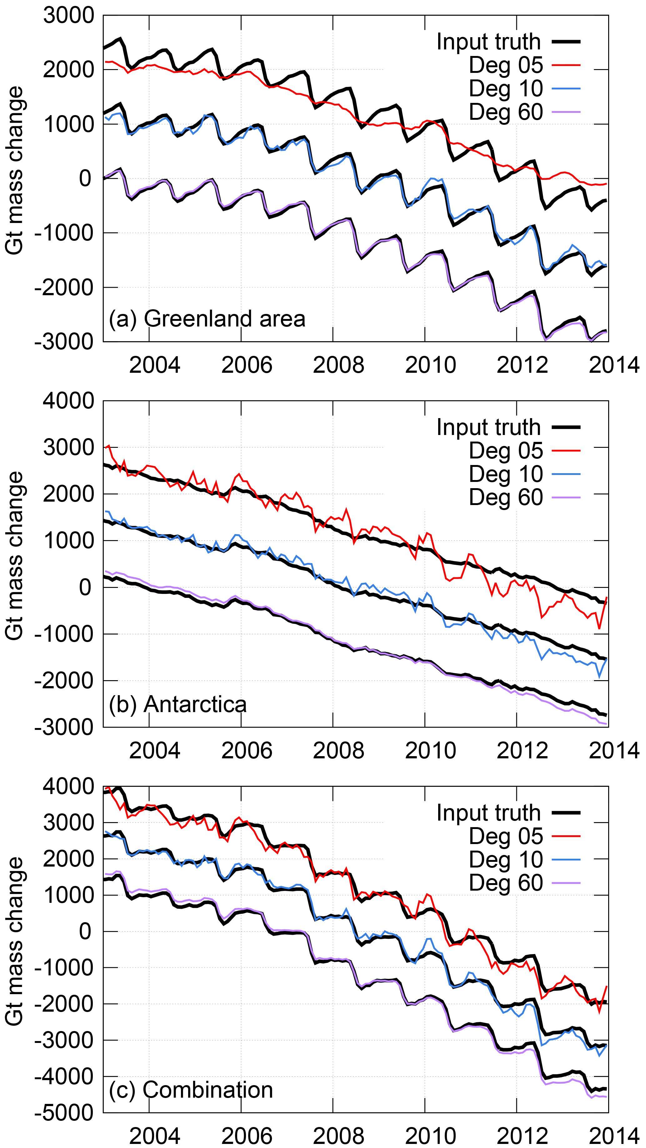
Figure 2Simulated inversion results by maximum degree/order, relative to input “truth” signal. Regions considered are (a) Greenland and surrounding islands, (b) Antarctica, and (c) the sum of Greenland and Antarctica. Each inversion was run using correlation-based constraints. Time series are offset for clarity.
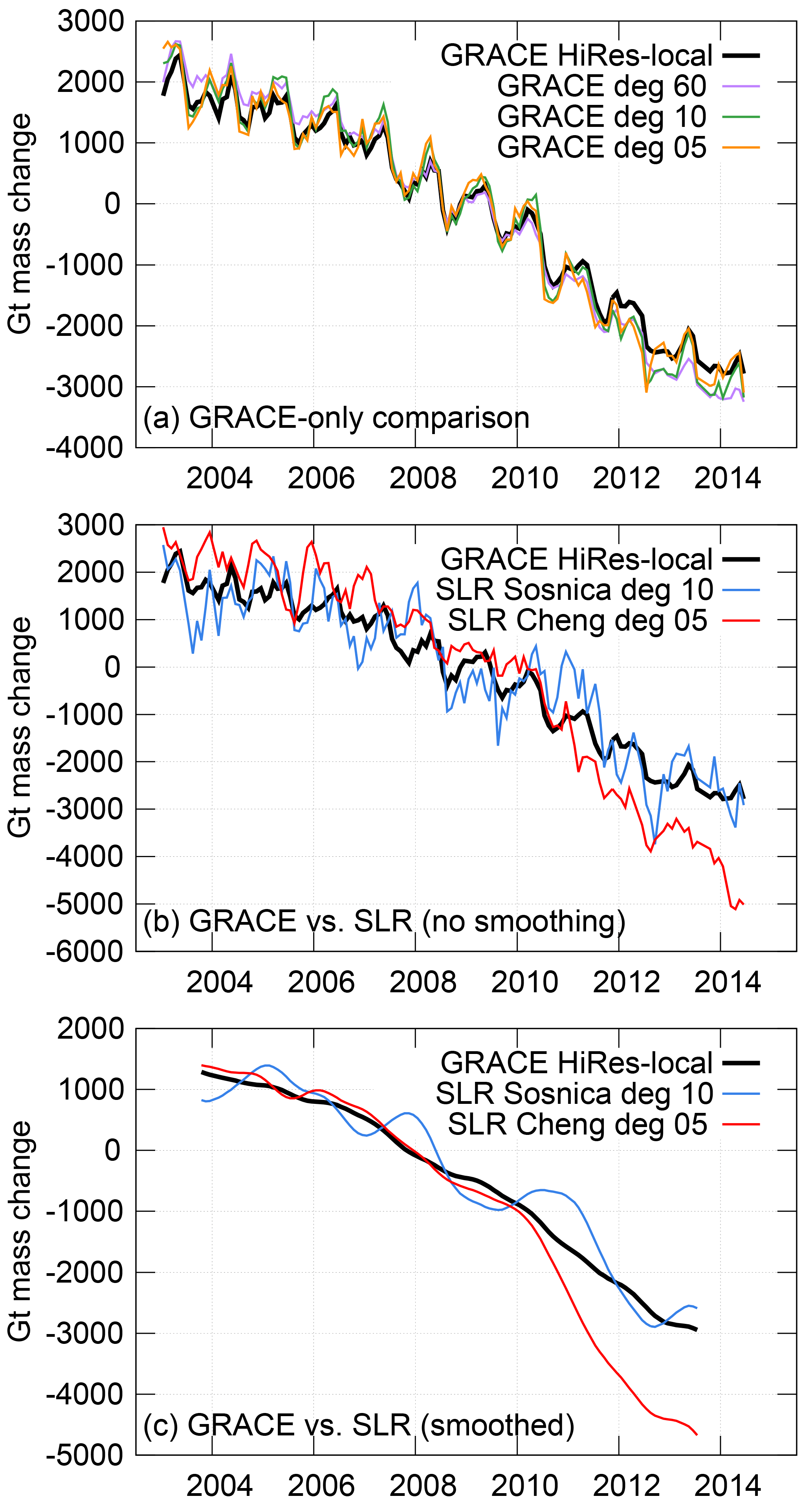
Figure 3Comparisons of inverted GRACE and SLR mass signals, over Greenland and Antarctica combined. (a) GRACE-only comparison, for different maximum degree/orders, relative to the high-resolution, local GRACE inversion. (b) SLR comparison. (c) Low-pass SLR comparison, after applying a 400-day (13 month) smoother.
Before enacting any inversion in the spatial domain, we wish to understand how similar these three SLR series are to the GRACE series, over the limited spherical harmonics they contain. To demonstrate this, we first smooth all time series for each gravity coefficient with a 200-day window, thus removing signals with semi-annual and shorter periods, which are likely to be noisy in both SLR and GRACE. We have plotted the GRACE, Cheng 5×5 SLR, and Sośnica 10×10 SLR series harmonic by harmonic in the Supplement. We then compute the percent of the smoothed GRACE variance that is explained by each SLR series (Fig. 1) via the equation:
where var denotes the variance of either the GRACE series or the residual once SLR is subtracted. A percent variance explained (PVE) of one means perfectly matching signals, a PVE of zero means that removing SLR does not reduce the GRACE variance, and a negative PVE means that the residual actually has more variability than the original GRACE series did. Ideally, we would want our PVEs to be above zero for all harmonics and near to one for the largest and most important harmonics.
We find that around half of the GRACE signal is explained by SLR for the degree-2 harmonics, but that skill rapidly decreases with wavelength. Above degree 4, none of the three modern SLR series explain a large percentage of the GRACE signal. Many of the harmonics of degrees 3 and above have negative PVEs, demonstrating SLR's known low sensitivity to them. Additionally, while low-degree harmonics from truncated GRACE series are well separated from the higher-degree coefficients, lower-degree SLR harmonics will inherently contain aliased errors from the unsolved-for higher-degrees.
The Sośnica 10×10 and Cheng 5×5 series have generally comparable PVEs at the lower degrees. While the Sośnica 6×6 data are similar to the Sośnica 10×10 data at degrees 2–3, it explains significantly less of the GRACE variance for degrees 4–6. For that reason, we focus on the other two series in this paper. The Cheng 5×5 series is particularly useful in this study because of its much longer record, but the independent nature of the Sośnica 10×10 makes it valuable for comparison.
To localize the mass signal from the low-resolution GRACE and SLR series to areas near Greenland and Antarctica, we use a modified version of the inversion technique described in Bonin and Chambers (2013). In that paper, a series of regions are defined ahead of time, and a least squares approach constrained by process noise is used to estimate the amount of mass change arising in each region. We attempted to use the same approach here, but quickly found that what can be done with 60×60 data sets cannot be accomplished with lower-resolution 5×5 data (see Supplement).
Instead, we use a correlation-based approach to constrain the least squares inversion. We first separate the world into three main areas: Antarctica, the ice-covered area near and including Greenland, and everything else. We divide each large area into multiple subregions, then tie those subregions loosely together with spatial and temporal constraints. This allows different subregions, such as eastern vs. western Antarctica, to vary at different times, while still keeping the number of observations significantly greater than the number of independent parameters solved for, thus giving a stable solution. The constraints are based on the JPL (Jet Propulsion Lab) mascon GRACE data (Watkins et al., 2015) from 2003 to 2014, after GIA has been removed. We compute cross-correlations between subregions within each area from the mascon data and use them to constrain the subregions so that they vary in expected spatial patterns. We also use lag-1 auto-correlations of each subregion to force each month's solution towards the neighboring months. The derivation of the constrained inversion process is given in the Supplement.
We first tested the process on a completely simulated data set, similar to the one used in Bonin and Chambers (2013). The details of the simulated data are given in the Supplement. The results suggest using a correlation-constrained least squares inversion that allows for accurate estimates of the Greenland and Antarctic mass change when using 60×60 or even 10×10 simulated data. However, a 5×5 resolution proves insufficient to invert the subannual signals correctly (Fig. 2a and b). We believe that this inaccuracy comes about because both Greenland and Antarctica are polar areas, and thus heavily dependent upon the same very low-degree spherical harmonics. Without higher-degree harmonics to clarify the situation, the mathematics cannot always determine which region to place which signal in.
We can eliminate this problem by summing the time series of the two areas and looking at the total mass loss over Antarctica and the near-Greenland area combined (Fig. 2c). Using SLR-like 5×5 harmonics for the simulation results in a negligible simulated trend error (7±18 Gt yr−1). The 60×60 simulated inversion produces a small trend error of 36±8 Gt yr−1 (6.5 % of the simulated “truth” trend). After removing these trends, the remaining RMS error of the correlation-constrained simulation inversion is 202±10 Gt for 5×5 data, 131±10 Gt for 10×10 data, and just 37±5 Gt for 60×60 data, which demonstrates that higher-resolution series are much better able to track the month-to-month variability within the data. (All errors given have 95 % confidence levels, based on a Monte Carlo simulation of random noise with a known red spectrum, after fitting for a bias, trend, annual, and semi-annual signals. The Monte Carlo simulation values are generated using the same RMS and lag-1 autocorrelation as the inverted data.)
Based on the results of the simulation, we applied the least squares inversion technique with correlation-based constraints to the real SLR and GRACE data and summed over all of Antarctica and the near-Greenland area. The resulting mass change time series are shown in Fig. 3. For a comparison truth signal, we use a combination of two higher-resolution inversions of the 60×60 GRACE data, which invert over only Antarctica and Greenland individually, and places each local signal into more, smaller regions. This technique estimates the mass trends and higher-resolution signals more accurately than the larger-region correlated technique can, since its regions and parameters are tuned for the full 60×60 data rather than 5×5 data (see Supplement). This allows for a more realistic estimate of the SLR errors. Also, since part of our goal is to match up the SLR time series with a high-quality GRACE one, learning the mismatch between them is important on its own.
We first consider the errors implicit in reducing the locally defined, high-resolution GRACE inverted series (black line in Fig. 3a) to a 5×5 truncated series (orange line). We find an error of 31.7 Gt yr−1 in trend (7.0±2.5 % of the high-resolution GRACE trend), such that between 2003 and 2014, the 5×5 GRACE inversion estimates 380 Gt greater total polar mass loss. Over that same time, the remaining RMS difference between the 5×5 and high-resolution GRACE inverted signals after the trends are removed is 220 Gt (63.7 %). These numbers are fairly comparable to our 5×5 simulation-based errors of 1.3±1.6 % for the trend and 75.1 % for the RMS. We should thus expect to see errors on this level from any SLR series, simply due to the signal truncation effect.
Table 1Differences relative to GRACE 60×60 high-resolution, local inversion, over the combined Greenland/Antarctica region during 2003–2014. Residual RMS errors are those after the trend has been removed, relative to the GRACE 60×60 detrended RMS. The final column is the residual RMS error after a 13-month Gaussian filter has been applied to all series. Errors given are at purely statistical 95 % confidence levels after fitting for a bias, trend, annual, and semi-annual signals, based on a Monte Carlo simulation of random red noise with the given RMS and lag-1 autocorrelations. They do not include the intrinsic errors of the satellites themselves or the effects of the inversion method. Errors are computed on series including only those months estimated by GRACE.
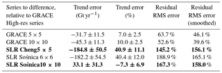
Figure 3b shows the inversion of the SLR series compared to GRACE, over only those months in which both SLR and GRACE data exist. The trend differences between GRACE and the Cheng 5×5 SLR series are particularly startling (40.9±11.1 % error), especially considering that the Sośnica 10×10 time series has a trend error of similar size to that caused by simple truncation to 5×5 harmonics (7.3 %). However, when the trend is removed, large and variable RMS errors (145–167 %) remain in both. We smoothed both the GRACE and SLR time series with a Gaussian smoother that cuts off periods shorter than 13 months (Fig. 3c; final column of Table 1) to remove month-to-month jitter and get a better view of what is causing the differences.
From 2003 to 2010, the Cheng 5×5 series sees very similar trends to the high-resolution GRACE series; the difference between their trends is statistically indistinguishable from zero. Then, from 2010 to 2014, the Cheng SLR and GRACE trends diverge suddenly and significantly (106.1±28.6 % trend difference). Collectively, this results in a 40.9 % error from 2003 to 2014. The Sośnica 10×10 inversion shows no such sudden change in behavior. This divergence in the Cheng SLR data seems so sudden that we initially believed it might have been caused by the pole-tide error discussed by Wahr et al. (2015). Their correction is a two-piece affair, treating the C21 and S21 harmonics differently before and after 2010, and its impact is largely linear. However, after applying the correction to our GRACE data, we realized that no pole-tide correction is large enough to explain the differences we see between GRACE and the Cheng SLR series. As Wahr et al. noted, the impact of their correction is on the order of 0.5 cm yr−1 equivalent water thickness in trend throughout the world. Trends in Greenland and Antarctica are 2 or 3 orders of magnitude greater than that.
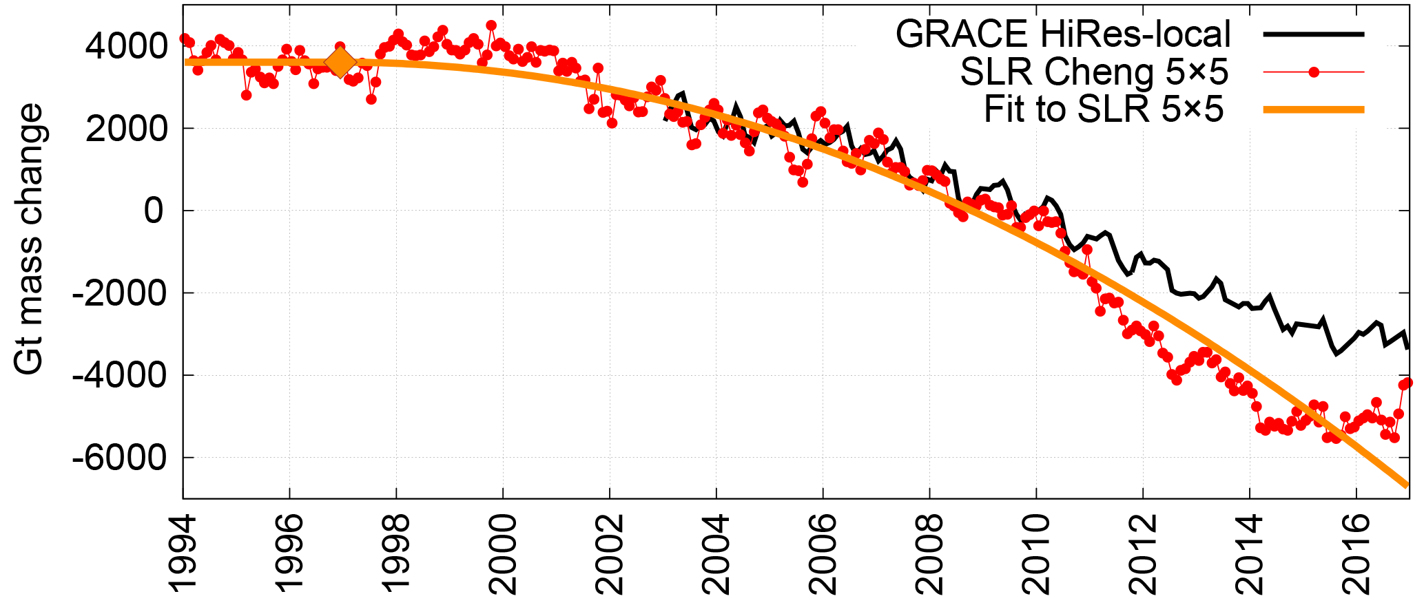
Figure 4Mass loss over Greenland and Antarctica combined, carried back to 1994, from the Cheng 5×5 SLR inversion. Monthly results are shown as red dots with the best-fit accelerating curve sketched in orange. The orange diamond represents the point at which acceleration begins. The high-resolution, local GRACE inversion beginning in 2003 is shown (black) for comparison.
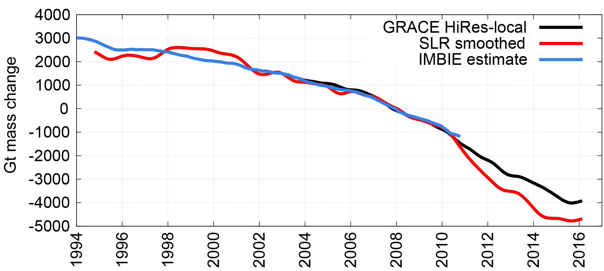
Figure 5The high-resolution localized GRACE (black), Cheng 5×5 SLR (red), and IMBIE (blue) estimates of Greenland and Antarctica's mass change. A 13-month smoother has been applied to the GRACE and SLR results, and they are scaled to include only the areas of Antarctica and Greenland, not the islands surrounding Greenland, to duplicate the IMBIE approach.
So instead of representing a true, long-term error in trend, the large interannual differences between GRACE and the Cheng 5×5 SLR series are probably indicative of a systematic interannual-scale error in the SLR inversion, which cannot be well quantified given the relatively short length of the GRACE record. This is most likely an indication of real differences in the SLR vs. GRACE data, not something caused by the processing technique itself, as trend errors from the inversion method are expected to be just 1.3±1.6 % (see Table S1 in the Supplement). Continuing the series past 2014 (Fig. 4) encourages us in this belief, since the SLR series measures effectively zero trend in mass change for 2014–2016, bringing it back towards the GRACE series. The Sośnica 10×10 series also differs significantly from GRACE on the interannual scale, despite the good agreement in trend. Its pattern of difference is more sinusoidal, with 2- to 3-year periods on top of a small but more-or-less constant trend difference. On an even shorter scale, the Cheng and Sośnica SLR series both resolve large annual-scale and shorter fluctuations that GRACE does not see. Since the SLR series do not see the same changes in either annual or multiyear signals as either each other or GRACE, we presume that the differences are most likely errors in SLR, though it is possible that GRACE contains unsuspected large interannual errors as well.
We did consider the impact of replacing the GRACE C20 term with that from a series related to the Cheng 5×5 SLR data. To test whether this unfairly biased the Cheng 5×5 SLR results towards GRACE, we removed the C20 terms completely from all of the GRACE and SLR series, then inverted each of them again. Removing the impact of the equatorial bulge greatly reduced the trend of each Greenland and Antarctica inverted series, but it did not significantly impact the interannual differences between GRACE and any SLR series. We thus conclude that the replacement of GRACE's C20 values is not a large contributing factor to these results.
It is disappointing but not a tremendous surprise that the SLR series cannot fully resolve the varying nature of the polar mass signal. GRACE is a rather high-resolution data set, while as Fig. 1 demonstrates, only the lowest-degree part of the SLR estimates are likely to be highly accurate. Our simulation showed that we are already pushing at the bounds of our spatial resolution to try localizing 5×5 data into even a single Greenland and Antarctic region, so one presumes that combining that difficulty with incorrect higher-degree values in SLR results in the large interannual errors that we see. Certainly, those errors mean that a 5×5 SLR field cannot be used to fill in gaps in the GRACE/GRACE Follow-On record.
However, in a longer-term sense and bearing in mind the limitations of the data, SLR does a fair job of estimating ice mass change. The Sośnica 10×10 series is not available much before GRACE or after 2014, but we can compute the Cheng 5×5 SLR inversion back to 1994 and through to the beginning of 2017 (Fig. 4). The most recent years of data show that the sharp divergence beginning in 2010 is recovering by 2017. (The lack of other satellite or in situ evidence for an increased mass loss from 2010 to 2014, and a stable mass state since then, makes us certain that SLR is less accurate than GRACE over this time span.) If this recovery continues, it will not represent a trend error, but an interannual error with a divergent period of around 5 years. Given that suggestive evidence, it is possible that the Cheng SLR series is broadly accurate on the 1994–2017 timescale, even though any individual year's estimate could be fairly far off.
The Cheng 5×5 SLR series' constant 23-year trend is Gt yr−1 for the combination of Greenland and Antarctica. However, a single line is an extremely poor approximation for this longer, sharply curving data set. If we instead assume that the ice sheets are in a long-term stable state at the beginning of 1994, then we can determine a constantly accelerating curve at an optimal point along the 1994–2017 SLR data (orange line in Fig. 4). The best two-piece fit to the data involves a constant (zero mass change) part until December of 1996 (±5 months) followed by a constant acceleration of Gt yr−2 thereafter. As Fig. 4 shows, even this model exaggerates the amount of mass that SLR sees lost after 2016 – an effect which would not occur if the Cheng SLR series did not diverge from GRACE beginning in 2010.
The obvious question we need to answer is how often SLR takes such multiyear excursions, and whether it really does get back on track afterwards. One way to get a feel for the pre-GRACE accuracy of the SLR inversion is via a comparison with an additional data set. The Ice-sheet Mass Balance Inter-comparison Exercise (IMBIE) for Greenland and Antarctica (http://imbie.org/data-downloads) (Shepherd et al., 2012) is a time series of mass change created from a combination of different techniques and data sources. This ensemble average includes radar altimetry over the whole timespan, and laser altimetry and GRACE after 2003. It also includes time series made with the model-based input–output method (estimates of precipitation minus runoff, sublimation, and ice discharge). It does not exist over the islands near Greenland which we included in our estimate, principally including Iceland, Svalbard, Ellesmere Island, and Baffin Island. To make a fair comparison, we mask out these neighboring islands from our final gridded solution, so that they are compared across the same area, then compute the summed mass change over Antarctica and Greenland. For visual purposes, we also smooth both GRACE and SLR with a 13-month Gaussian smoother to duplicate what was done with IMBIE. One significant difference remaining is that IMBIE naturally includes the impact of the geocenter terms, while we have excluded those from our SLR estimate because of their large expected errors.
As Fig. 5 demonstrates, IMBIE's mass change estimate aligns neatly with GRACE during its 6-year overlapping time span, but also approximates a similar long-term signal to SLR before GRACE. During the overlapping 15-year period (1994–2009), the Cheng 5×5 SLR inversion estimates an average mass loss rate of Gt yr−1, while IMBIE sees a statistically identical trend of Gt yr−1. (The IMBIE uncertainty here is based on the variance of the smoothed residuals about the fit, but also accounts for temporal correlation due to the 13-month smoothing already applied to the IMBIE data. This reduces degrees of freedom from 186 to 14, so inflates the error from the least squares fit by .) Assuming IMBIE is correct, the SLR inversion sees multiyear errors before 2002, as it does from 2010 to 2017. However, over the long-term, these errors have averaged out in previous similar cases, as they seem to be in the process of doing now.
We compared two unrelated SLR series to the GRACE data in the hope that one or the other would prove capable of reliably matching GRACE and estimating mass change over Greenland and Antarctica on its own. The Sośnica 10×10 series contains significant shorter-period discrepancies with GRACE, but estimates the 10-year trend with reasonable accuracy. Unfortunately, the Sośnica series does not exist before 2000 or after 2014, so it cannot currently be tested over longer scales. It would potentially be possible to use the Sośnica method to extend the series – but with a caveat. The creators of this series included not only the five long-running geodetic satellites in their solution, but also BLITS, Larets, Beacon-C, and LARES over the time spans in which they have existed. Beacon-C is the only one of those satellites which has existed before 2000, and it has been heavily downweighted. Larets first enters into the solution in September of 2003, BLITS in September of 2009, and LARES not until February of 2012. So, we expect the signal quality to be degraded prior to 2003, leading to pre-GRACE estimates of mass change which may be of low accuracy. On the other hand, since 2012, the Sośnica technique should have produced a solution comparable to or better than what is shown in Fig. 3 and Table 1. An extended Sośnica-like series might, therefore, be useful for filling the gap between GRACE and GRACE Follow-On.
The Cheng 5×5 series already exists for the full 1994–2017 time period. However, because of the large uncertainty on interannual periods, we do not believe the Cheng 5×5 inverted SLR data series should be used to estimate mass loss over Greenland and Antarctica on its own. Certainly, we cannot use it to fill short-term gaps in the GRACE record or between the GRACE and the future GRACE Follow-On missions. Nonetheless, over longer time spans (∼20 years), the inverted Cheng 5×5 SLR series appears to measure real mass change signal, similar to the more extensive IMBIE estimates. It (or an extended Sośnica-like series) thus ought to be considered in combination with other data sources in the future. In an attempt to make SLR more useful for this effort, our future work will include the creation of a new SLR series, created in the same manner as the Cheng 5×5 series, but including a year of data in each estimate, rather than a month. The hope is that, by sacrificing the subannual signal, we can gain better accuracy for interannual periods, thus reducing the variability which stymies us here and creating a more useful pre-GRACE estimate of total mass change over Greenland and Antarctica.
The monthly Cheng 5×5 SLR data are available as part of the Supplement and are online at https://doi.org/10.5281/zenodo.831745. All other data series are publicly available at the websites listed in the text. The numerical inversion results or mapped regional definitions are available from the authors upon request.
The supplement related to this article is available online at: https://doi.org/10.5194/tc-12-71-2018-supplement.
We would like to deeply thank John Ries at the University of Texas Center for Space Research for his kind assistance in the preparation of this paper. Thank you so much for sharing your generous SLR background knowledge and advice with us.
This research was conducted under a New (Early Career) Investigator Program
in Earth Science NASA grant (NNX14AI45G). We are most appreciative of NASA's
funding and support.
Edited by: Etienne Berthier
Reviewed by: Kosuke HEKI and one anonymous referee
A, G., Wahr, J., and Zhong, S.: Computations of the viscoelastic response of a 3-D compressible earth to surface loading: an application to glacial isostatic adjustment in Antarctica and Canada, Geophys. J. Int., 192, 557–572, https://doi.org/10.1093/gji/ggs030, 2013.
Bettadpur, S.: UTCSR Level-2 Processing Standards Document (for Level-2 Product Release 0005), GRACE 327–742, CSR Publ. GR-12-xx, Rev. 4.0, University of Texas, Austin, 2012.
Bonin, J. and Chambers, D.: Uncertainty estimates of a GRACE inversion modelling technique over Greenland using a simulation, Geophys. J. Int., 194, 212–229, https://doi.org/10.1093/gji/ggt091, 2013.
Chambers, D. P.: Observing seasonal steric sea level variations with GRACE and satellite altimetry, J. Geophys. Res.-Oceans, 111, C03010, https://doi.org/10.1029/2005JC002914, 2006.
Chambers, D. P. and Bonin, J. A.: Evaluation of Release-05 GRACE time-variable gravity coefficients over the ocean, Ocean Sci., 8, 859–868, https://doi.org/10.5194/os-8-859-2012, 2012.
Cheng, M.: Laser ranging in 5×5 spherical harmonics, Zenodo, https://doi.org/10.5281/zenodo.831745, 2017.
Cheng, M. and Ries, J.: The unexpected signal in GRACE estimates of C20, J. Geodesy, 91, 897–914, https://doi.org/10.1007/s00190-016-0995-5, 2017.
Cheng, M., Ries, J. C., and Tapley, B. D.: Variations of the Earth's figure axis from satellite laser ranging and GRACE, J. Geophys. Res.-Sol. Ea., 116, B01409, https://doi.org/10.1029/2010JB000850, 2011.
Cheng, M. K., Ries, J. C., and Tapley, B. D.: Geocenter Variations from Analysis of SLR data, from Reference Frames for Applications in Geosciences, International Association of Geodesy Symposia, Springer-Verlag, Berlin Heidelberg, vol. 138, 19–36, 2013.
Collilieux, X., Altamimi, Z., Ray, J., Van Dam, T., and Wu, X.: Effect of the satellite laser ranging network distribution on geocenter motion estimation, J. Geophys. Res.-Sol. Ea., 114, 1–17, https://doi.org/10.1029/2008JB005727, 2009.
Howat, I. M., Smith, B. E., Joughin, I., and Scambos, T. A.: Rates of southeast Greenland ice volume loss from combined ICESat and ASTER observations, Geophys. Res. Lett., 35, 1–5, https://doi.org/10.1029/2008GL034496, 2008.
Jacob, T., Wahr, J., Pfeffer, W. T., and Swenson, S.: Recent contributions of glaciers and ice caps to sea level rise., Nature, 482, 514–518, https://doi.org/10.1038/nature10847, 2012.
Johannessen, O. M., Khvorostovsky, K., Miles, M. W., and Bobylev, L. P.: Recent ice-sheet growth in the interior of Greenland, Science, 310, 1013–1016, https://doi.org/10.1126/science.1115356, 2005.
Luthcke, S. B., Sabaka, T. J., Loomis, B. D., Arendt, A. A., McCarthy, J. J., and Camp, J.: Antarctica, Greenland and Gulf of Alaska land-ice evolution from an iterated GRACE global mascon solution, J. Glaciol., 59, 613–631, https://doi.org/10.3189/2013JoG12J147, 2013.
Matsuo, K., Chao, B. F., Otsubo, T., and Heki, K.: Accelerated ice mass depletion revealed by low-degree gravity field from satellite laser ranging: Greenland, 1991–2011, Geophys. Res. Lett., 40, 4662–4667, https://doi.org/10.1002/grl.50900, 2013.
Nerem, R. S. and Wahr, J.: Recent changes in the Earth's oblateness driven by Greenland and Antarctic ice mass loss, Geophys. Res. Lett., 38, 1–6, https://doi.org/10.1029/2011GL047879, 2011.
Nerem, R. S., Eanes, R. J., Thompson, P. F., and Chen, J. L.: Observations of annual variations of the earth's gravitational field using satellite laser ranging and geophysical models, Geophys. Res. Lett., 27, 1783–1786, https://doi.org/10.1029/1999GL008440, 2000.
Rignot, E., Velicogna, I., van den Broeke, M. R., Monaghan, A., and Lenaerts, J. T. M.: Acceleration of the contribution of the Greenland and Antarctic ice sheets to sea level rise, Geophys. Res. Lett., 38, L05503, https://doi.org/10.1029/2011GL046583, 2011.
Sasgen, I., van den Broeke, M., Bamber, J. L., Rignot, E., Sørensen, L. S., Wouters, B., Martinec, Z., Velicogna, I., and Simonsen, S. B.: Timing and origin of recent regional ice-mass loss in Greenland, Earth Planet. Sc. Lett., 333–334, 293–303, https://doi.org/10.1016/j.epsl.2012.03.033, 2012.
Schrama, E. J. O. and Wouters, B.: Revisiting Greenland ice sheet mass loss observed by GRACE, J. Geophys. Res.-Sol. Ea., 116, B02407, https://doi.org/10.1029/2009JB006847, 2011.
Shepherd, A., Ivins, E. R., A, G., Barletta, V. R., Bentley, M. J., Bettadpur, S., Briggs, K. H., Bromwich, D. H., Forsberg, R., Galin, N., Horwath, M., Jacobs, S., Joughin, I., King, M. A., Lenaerts, J. T. M., Li, J., Ligtenberg, S. R. M., Luckman, A., Luthcke, S. B., McMillan, M., Meister, R., Milne, G., Mouginot, J., Muir, A., Nicolas, J. P., Paden, J., Payne, A. J., Pritchard, H., Rignot, E., Rott, H., Sørensen, L. S., Scambos, T. A., Scheuchl, B., Schrama, E. J. O., Smith, B., Sundal, A. V., van Angelen, J. H., van de Berg, W. J., van den Broeke, M. R., Vaughan, D. G., Velicogna, I., Wahr, J., Whitehouse, P. L., Wingham, D. J., Yi, D., Young, D., and Zwally, H. J.: A reconciled estimate of ice-sheet mass balance, Science, 338, 1183–1189, https://doi.org/10.1126/science.1228102, 2012.
Sośnica, K., Jäggi, A., Meyer, U., Thaller, D., Beutler, G., Arnold, D., and Dach, R.: Time variable Earth's gravity field from SLR satellites, J. Geodesy, 89, 945–960, https://doi.org/10.1007/s00190-015-0825-1, 2015.
Swenson, S., Chambers, D., and Wahr, J.: Estimating geocenter variations from a combination of GRACE and ocean model output, J. Geophys. Res.-Sol. Ea., 113, B08410, https://doi.org/10.1029/2007JB005338, 2008.
Talpe, M. J., Nerem, R. S., Forootan, E., Schmidt, M., Lemoine, F. G., Enderlin, E. M., and Landerer, F. W.: Ice mass change in Greenland and Antarctica between 1993 and 2013 from satellite gravity measurements, J. Geodesy, 91, 1283–1298, https://doi.org/10.1007/s00190-017-1025-y, 2017.
Tapley, B. D., Bettadpur, S., Ries, J. C., Thompson, P. F., and Watkins, M. M.: GRACE measurements of mass variability in the Earth system, Science, 305, 503–505, https://doi.org/10.1126/science.1099192, 2004.
Velicogna, I. and Wahr, J.: Time-variable gravity observations of ice sheet mass balance: precision and limitations of the GRACE satellite data, Geophys. Res. Lett., 40, 3055–3063, https://doi.org/10.1002/grl.50527, 2013.
Wahr, J., Nerem, R. S., and Bettadpur, S. V: The pole tide and its effect on GRACE time-variable gravity measurements: implications for estimates of surface mass variations, J. Geophys. Res.-Sol. Ea., 120, 4597–4615, https://doi.org/10.1002/2015JB011986, 2015.
Watkins, M. M., Wiese, D. N., Yuan, D., Boening, C., and Landerer, F. W.: Improved methods for observing Earth's time variable mass distribution with GRACE using spherical cap mascons, J. Geophys. Res.-Sol. Ea., 120, 1–24, https://doi.org/10.1002/2014JB011547, 2015.
Whitehouse, P. L., Bentley, M. J., Milne, G. A., King, M. A., and Thomas, I. D.: An ew glacial isostatic adjustment model for Antarctica: calibrated and tested using observations of relative sea-level change and present-day uplift rates, Geophys. J. Int., 190, 1464–1482, https://doi.org/10.1111/j.1365-246X.2012.05557.x, 2012.
Wu, X., Ray, J., and van Dam, T.: Geocenter motion and its geodetic and geophysical implications, J. Geodyn., 58, 44–61, https://doi.org/10.1016/j.jog.2012.01.007, 2012.