Decadal changes of surface elevation over permafrost area estimated using reflected GPS signals

Conventional benchmark-based survey and Global Positioning System (GPS) have been used to measure surface elevation changes over permafrost areas, usually once or a few times a year. Here we use reflected GPS signals to measure temporal changes of ground surface elevation due to dynamics of the active layer and near-surface permafrost. Applying the GPS interferometric reflectometry technique to the multipath signal-to-noise ratio data collected by a continuously operating GPS receiver mounted deep in permafrost in Barrow, Alaska, we can retrieve the vertical distance between the antenna and reflecting surface. Using this unique kind of observables, we obtain daily changes of surface elevation during July and August from 2004 to 2015. Our results show distinct temporal variations at three timescales: regular thaw settlement within each summer, strong interannual variability that is characterized by a sub-decadal subsidence trend followed by a brief uplift trend, and a secular subsidence trend of 0.26 ± 0.02 cm year⁻¹ during 2004 and 2015. This method provides a new way to fully utilize data from continuously operating GPS sites in cold regions for studying dynamics of the frozen ground consistently and sustainably over a long time.

1 Introduction

Over permafrost terrains the ground surface undergoes seasonal vertical deformation due to the water/ice-phase changes occurring in annual freeze–thaw cycles. Superimposed on the seasonal cycle, interannual and long-term changes of ground surface elevation may occur due to permafrost degradation/aggradation and subsurface water migration. Measuring and monitoring surface elevation changes at various timescales is critical to (1) improving our understanding of the dynamics of the integrated system of permafrost and the active layer (i.e., the seasonally freezing/thawing layer on top of permafrost), (2) studying the impacts of permafrost changes on hydro-ecological systems, and (3) assessing the risk of permafrost changes to infrastructure such as buildings and roads.

Measurements of surface elevation changes over permafrost areas have been largely based on conventional benchmark-based surveys. The classical method is to use vertical tubes or pipes anchored deep in permafrost as datum benchmarks of the ground surface for repeat leveling surveys (e.g., Mackay and Burn, 2002). Mackay also developed a few instruments such as the “heavemeter” (also called heave tube), magnet probe, and access tube, specifically for measuring frost heave (Mackay, 1983; Mackay and Leslie, 1987). Using linear variable differential transformers, Harris et al. (2007) designed an instrument for monitoring solifluction movement, including surface elevation changes, in Svalbard.

Advancing from conventional to space geodetic methods, Little et al. (2003) carried out one of the first differential Global Positioning System (GPS) campaigns on tundra surface over permafrost areas. Placing the GPS antenna on the top of specially designed tubes, they measured the surface vertical positions in the summers of 2001 and 2002 at two sites in the Kuparuk River basin, Alaska. The Circumpolar Active Layer Monitoring (CALM) program adopted the same protocol and conducted decade-long GPS campaigns at the end of thaw seasons in three continuous permafrost areas in northern Alaska (Shiklomanov et al., 2013; Streletskiy et al., 2017). However, these campaigns have been only conducted annually in mid- or late August, and thus do not allow one to measure seasonal changes.

In recent years, modern remote sensing methods have been utilized for mapping vertical deformation over permafrost areas. Interferometric synthetic aperture radar (InSAR) has been used to quantify permafrost subsidence at both seasonal and decadal timescales (Liu et al., 2010, 2014, and 2015). However, InSAR suffers from relatively long repeat intervals (6 to 46 days, depending on the satellite platforms) and loss of interferometric coherence for mapping multiple-year changes over permafrost areas. Moreover, InSAR measurements are fundamentally relative and need to be tied to a reference point, where the deformation is known or can be assumed to be zero. Furthermore, it is difficult to locate stable reference points in permafrost areas where bedrock outcrops are absent. Differential digital elevation models constructed from stereographic images or lidar have revealed subsidence due to permafrost degradation (Lantuit and Pollard, 2005; Jones et al., 2013, 2015; Günther et al., 2015). However, these measurements were conducted at annual or multi-year intervals, and the accuracy of elevation changes are on the order of sub-meters. Ground-based remote sensing tools, such as terrestrial laser scanning and ground-based InSAR, are emerging methods for measuring permafrost-related deformation within close ranges (Strozzi et al., 2015; Liu et al., 2016; Luo et al., 2017). However, most of these field campaigns have focused on slope movements such as rock glacier flow and retrogressive thaw slumps.

In this study, we apply the GPS interferometric reflectometry (GPS-IR) technique (Larson et al., 2008, 2009) to the signal-to-noise ratio (SNR) data collected by a continuously operating GPS receiver in Barrow, Alaska. This technique can retrieve the vertical distance between the antenna and reflecting surface. We will demonstrate that such a GPS-IR observable directly reflects the surface elevation changes due to dynamics of the frozen ground. We generate a time series of daily surface elevation changes on snow-free days over 12 summers. We will show that our observed interannual and decadal elevation changes match well with the GPS campaign observations from Streletskiy et al. (2017) at a nearby site.

2 Key processes for vertical surface movement over flat terrains in continuous permafrost

In areas underlain by continuous permafrost, vertical movement at the ground surface is largely related to the phase and volumetric change of ground ice. Here we briefly summarize the key processes for gradual vertical movement over flat terrains in continuous permafrost areas at annual, sub-decadal, and multi-decadal timescales.

At annual timescales, the active layer freezes and thaws. In the early freezing stage, water in the pore space freezes locally to pore ice. Such a phase change causes a volume expansion, resulting in surface uplift. Due to the cryosuction processes, liquid water (soil moisture) migrates towards the freezing front near the base of the active layer, freezes and forms ice lens, termed segregated (or segregational) ice (Smith, 1985; French, 2007). Ice segregation near the base of the active layer results in total frost heave that exceeds the potential 9 % volume expansion of all the water in the active layer. Conversely, in the following thaw season, pore and segregated ice within the active layer melts, volume decreases, and thaw consolidation causes the ground to settle.

At sub-decadal timescales, vertical movements are controlled by ice conditions just beneath the active layer. Numerous permafrost studies suggest the existence of an ice-rich transition layer located between the base of the active layer and the top of the permafrost (Shur et al., 2005). In the literature, some call the top of the transition layer the “transient layer”, which can alter its status between seasonally thawing and freezing and perennially frozen at sub-decadal scales (e.g., Shur et al., 2005; French, 2007). We use “transition layer” in this paper without further distinguishing the transient layer from it. At the end of an exceptionally warm summer, the active layer deepens beyond its normal thickness and the ice-rich transition layer may thaw. As a result, enhanced surface subsidence can occur. Conversely, during the years when segregated ice grows within the transition layer, it becomes thicker and causes surface uplift.

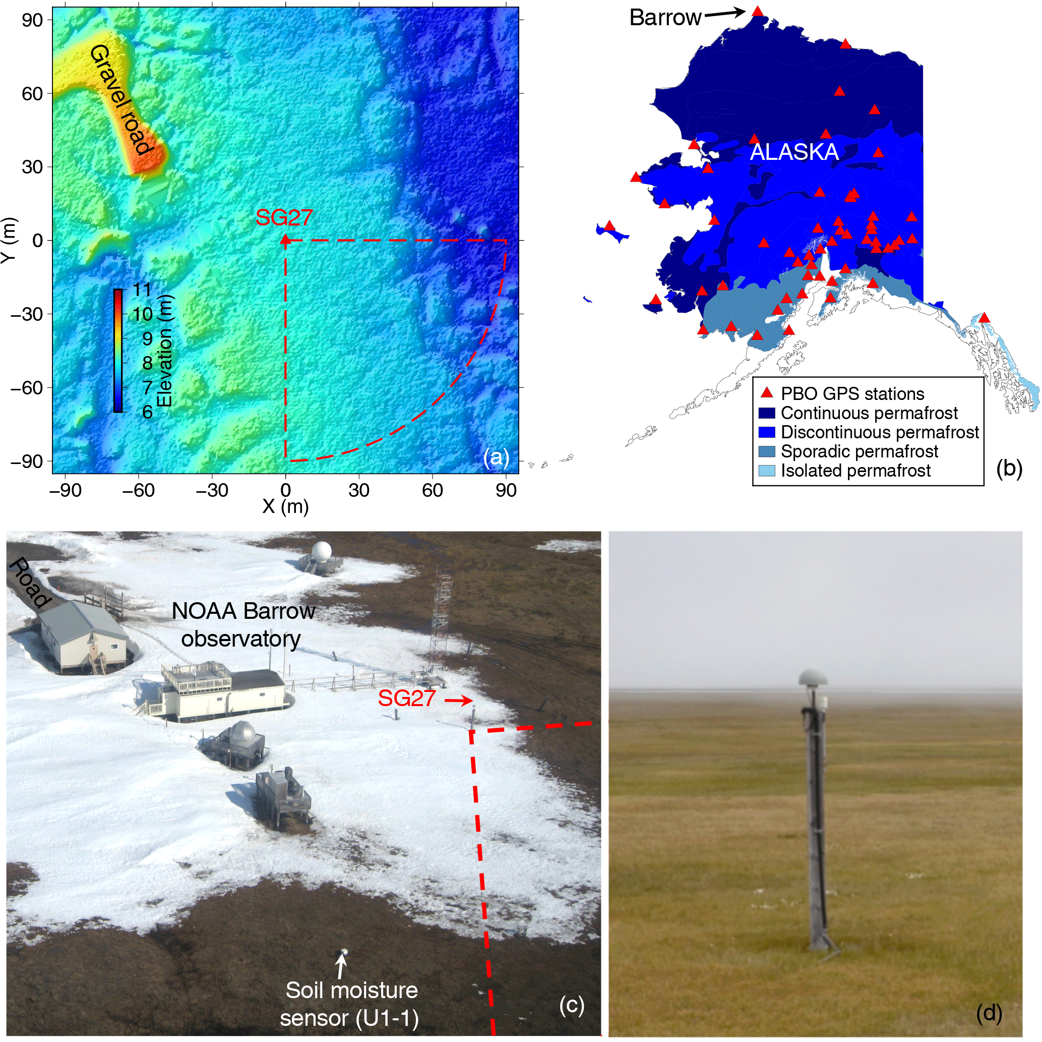
Figure 1 (a) Relief map of the area surrounding the GPS station SG27, produced using a lidar data set collected in August 2012 (Wilson et al., 2014). The x and y axes show horizontal and vertical positions relative to SG27 in UTM Zone 4N. The red dashed fan shape outlines the estimated footprint of the GPS reflected signals (see Sect. 4.2). (b) Permafrost extent in Alaska (after Brown et al., 1997). The red triangles denote the PBO GPS stations located in the permafrost areas. (c) Aerial photograph over the facilities of the NOAA Barrow Observatory and SG27 (photo: NOAA). The red dashed lines denote the western portion of the footprint. (d) A close-up photograph of SG27, viewing from the north (photo: Elchin Jafarov, August 2013).

Table 1 History of equipment changes at SG27. The equipment codes follow the International GNSS Service convention (ftp://ftp.igs.org/pub/station/general/rcvr_ant.tab).

If warming conditions persist for several decades or strong disturbances occur, the ice-rich transition layer could largely thaw, and permafrost degradation would begin. In areas where the near-surface permafrost is ice-rich, thermokarst processes could initiate at local scales upon thawing, causing abrupt and deep thaw as well as strong and irregular surface subsidence (Jorgenson, 2013). Recent observations from campaign GPS and InSAR reveal that thaw subsidence due to permafrost degradation can also occur gradually (a few millimeters per year) and relatively homogenously at regional scales (Liu et al., 2010; Shiklomanov et al., 2013; Streletskiy et al., 2017).

3 GPS station SG27 and permafrost conditions

The GPS station SG27 (156^∘36^′37${}^{\prime \prime }$ W, 71^∘19^′22${}^{\prime \prime }$ N) is in northern Barrow, next to the NOAA Barrow Observatory (Fig. 1). The GPS receiver is attached to a wooden monument that is ∼ 3.8 m above the ground surface. The bottom of the monument is about 5 m beneath the surface. The station has been continuously operating and receiving L1 GPS signals since May 2002. It started receiving L2C signals in 2013. SG27 underwent two major instrumental changes, first on 1 June 2004 and second on 26 August 2010 (Table 1). The vertical shift in the GPS antenna phase center in 2010 was only 2 mm, having negligible effects on our data analysis and interpretation. SG27 is part of the Plate Boundary Observatory (PBO) network (http://pboweb.unavco.org). The main objective of this network is to support the study of solid earth movement, especially plate tectonics. According to the circumpolar permafrost map of Brown et al. (1997), 58 Alaska PBO stations are located in permafrost zones (Fig. 1b). Among these, 14 and 19 sites are underlain by continuous and discontinuous permafrost, respectively.

The broad Barrow area is a flat coastal plain underlain by continuous permafrost. The upper part of the permafrost is ice-rich, with ice content of up to 75 % in the top 2 m (Brown and Sellmann, 1973). Characterized by Arctic maritime climate, the summer is cool and moist. The thaw season lasts from early June to early August (Shiklomanov et al., 2010). According to the 1987–2016 climatological mean, the snow-free period typically lasts from July to mid-August (Cox et al., 2017). The active layer is dominantly organic-rich soil that is nearly saturated during the thaw seasons (Shiklomanov et al., 2010).

Within 90 m of SG27 (the footprint of the reflected GPS signals; see Sect. 4.2), the ground surface is flat, homogenous, polygon-free upland, and unaffected by thermokarst processes (Fig. 1). The vegetation is mostly moist acidic tundra, typical for this region. The active layer thickness (ALT) in 2016 was 53 cm with a standard deviation of 6 cm, obtained from mechanic probing at six locations within 90 m of SG27 on 16 August 2016 (Go Iwahana, personal communication, 23 August 2016).

4 Methods

4.1 Data sets

In this subsection, we briefly summarize the key data sets we use in this study.

4.1.1 GPS data from SG27

The primary data are the multipath SNR data collected by SG27. We apply the GPS-IR analysis to these SNR data to estimate the ground elevation changes (see Sects. 4.2 and 5.2 for the data processing method and results, respectively). We also use the daily vertical positions of the GPS receiver as a secondary data set, for two purposes: (1) to illustrate the magnitude of solid earth movement in the vertical direction and (2) to correct for the solid earth contribution from the GPS campaign results of Streletskiy et al. (2017) so that we can directly compare theirs with our GPS-IR results (see more in Sect. 4.3). We simply adopt the GPS geodetic solutions published by the Nevada Geodetic Laboratory at the University of Nevada (http://geodesy.unr.edu/NGLStationPages/stations/SG27.sta). The vertical positions are in the North America Fixed Reference Frame (NA12), relative to the Earth system center of mass (Blewitt et al., 2013).

4.1.2 Surface elevation changes from the GPS campaigns of Streletskiy et al. (2017)

Streletskiy et al. (2017) conducted GPS campaigns and measured surface elevation in late August from 2003 to 2015 at four plots in the ice-wedge-dominated Cold Regions Research and Engineering Laboratory (CRREL) transect (∼ 2 km southeast of SG27). Their surface positions results are in the North American Datum of 1983 (NAD83), an Earth-centered (“geocentric”) ellipsoidal system. These campaign measurements provide a key data set for us to compare with our results (see more in Sect. 5.3).

4.1.3 Soil and meteorological data

We use two types of time-varying soil data, namely the ALT and soil moisture, to aid in quantitative interpretation of our GPS-IR results (Sect. 5). Since the early 1990s, the CALM program has been measuring ALT every mid-August at two sites: a regular 1 km by 1 km grid (site ID: U1; center coordinates: 156^∘35^′ W, 71^∘18^′ N) and the 2 km long CRREL transect. The mean ALT at the U1 site was about 36 cm between 2004 and 2015 and no significant trend in the past 20 years (Shiklomanov et al., 2010 and updated data from https://www2.gwu.edu/~calm/data/webforms/u1_f.htm). Soil moisture was measured nearly daily at the CALM soil–climate site U1-1, located approximately 60 m south-southeast of SG27 (Fig. 1c). The period of the publicly available soil moisture data is from late August in 1995 to the end of 2011.

We use the daily averaged 2 m air temperatures measured at the nearby NOAA Barrow Observatory to calculate thaw indices, which are then used to model seasonal subsidence (Sect. 4.4). We also use the daily precipitation measured at Barrow Airport to investigate the possible link between precipitation and subsidence (Sect. 5.4).

4.2 GPS interferometric reflectometry (GPS-IR)

GPS-IR is a technique that uses the interference between the direct and reflected GPS signals to infer ground properties such as snow depth, soil moisture, and vegetation water content (Larson et al., 2008, 2009; Small et al., 2010). Larson (2016) provides an overview of the GPS-IR technique. Here we only describe the method of using GPS-IR to measure the reflector height, which refers to the height of the GPS receiver antenna phase center above the reflecting surface.

GPS-IR uses the interference between the direct signal and the reflected signal from the ground surface. Figure 2 illustrates the interference geometry. The strength of the interference, quantified by the SNR of the received power, oscillates with the elevation angle (e). For a horizontal planar reflector, such as the flat surface surrounding SG27, the SNR oscillation is characterized by a dependency on sine of the elevation angle (Larson, 2016):

$$\begin{array}{}\text{(1)}& \mathrm{SNR}=A\sin \left({\displaystyle \frac{\mathrm{4}\mathit{\pi }H}{\mathit{\lambda }}}\sin e+\mathit{\varphi }\right),\end{array}$$

where A is the amplitude, H is the reflector height, λ is the wavelength of the GPS signal, and ϕ is the phase offset of the oscillation. Given a measure of varying SNR with sine, we calculate its periodogram using the Lomb–Scargle spectral analysis (Press et al., 1996), determine the dominant frequency f, and eventually obtain the reflector height H as fλ∕2. The reflection observed in SNR data using a geodetic antenna is most sensitive to the interface between air and the top soil layer.

Figure 2 Schematic diagram of the GPS-IR geometry. The sub-surface in Barrow is depicted by a simplified three-layer model that consists of the active layer (∼ 53 cm thick in August 2016), the transition layer (thickness unknown), and the permafrost layer (> 300 m thick). The top of permafrost is ice-rich.

We apply this method to the L1 SNR data (λ=0.19029 m) recorded by SG27 to retrieve the reflector height at daily intervals. Using the SNR data from individual satellite track with an elevation angle range of 5 to 20^∘, we estimate the reflector height and repeat this for all tracks. To avoid the obstructions from buildings and other infrastructure located nearby (Fig. 1c), we only keep the H with azimuth angles of 90 to 180^∘ (i.e., in the southeast quadrant). Then we average H from all usable tracks and use the average to represent the reflector height within the GPS-IR footprint. We calculate the standard error of the mean as the uncertainty of the averaged H. In fact, each track has a different reflecting point, which depends on the azimuth and elevation angles, as well as the antenna height. Using the first Fresnel zone of the reflected signals for the elevation angle of 5^∘ (Larson and Nievinski, 2013), we estimate the average extent of the footprints as having a radius of 90 m from SG27. To avoid the ambiguous interpretation about reflector height changes as caused by snow depth changes or by the thawing/freezing of soil, we only consider reflector height on snow-free days between 1 July and 31 August in each summer from 2004 to 2015. We exclude the data before 2004 to avoid a significant offset due to the GPS equipment change on 1 June 2004.

4.3 Surface elevation changes in a geocentric frame and contribution from solid earth movement

By combining the daily reflector height and the vertical position of the GPS receiver, we can calculate the change of ground surface elevation at SG27 in a geocentric frame. Let V be the vertical position of the GPS receiver, then the vertical position of the ground S is simply V minus H (Fig. 2). It is worth pointing out that in a geocentric frame, the surface elevation changes (from either our GPS-IR retrieval or the GPS campaigns) include contributions from two independent processes: one is due to the dynamics of the active layer and near-surface permafrost (referred to as “frozen ground dynamics”), and the other due to the movement of solid earth. Assuming the anchor position (P) is stable as it is deeply frozen in permafrost (at ∼ 5 m depth) and the wooden pole is rigid, any change of the receiver's vertical position (V) is due to the solid earth movement. This solid earth component needs to be removed for studying frozen ground dynamics. After this correction (i.e., subtracting by V), the surface elevation change due to frozen ground dynamics, denoted as S_F as a function of time t, is reduced to a simple negative relation with the reflector height:

$$\begin{array}{}\text{(2)}& S_{\mathrm{F}}\left(t\right)=-H\left(t\right).\end{array}$$

Therefore, the GPS-IR framework is intrinsically convenient: we only need the reflector height H, rather than the solid earth movement V, for studying frozen ground dynamics. If not explicitly stated, all surface elevation results presented and discussed in the remainder of this paper are given with the S_F(t) term in the geocentric NA12 frame. To directly compare S_F values retrieved using GPS-IR and those obtained by the GPS campaigns of Streletskiy et al. (2017), we first convert their vertical position values from NAD83 to NA12, then remove V measured at SG27 from theirs. The solid earth movement is nearly the same at SG27 and the sites of Streletskiy et al. (2017), within 2 km distance in this tectonically inactive area.

4.4 Modeling seasonal subsidence due to the melting of pore ice in the active layer

We also model seasonal ground surface subsidence due to the melting of pore ice in the active layer and further assess the subsidence from the melting of segregated ice. For simplicity, the following conceptual and mathematical framework is for a given thaw season. Our model only considers one component in the seasonal subsidence that is caused by the volume decrease from ice to water in the pores of the active layer as it thaws. Another component is the subsidence caused by thawing of segregated ice. We denote these two subsidence components as d_pore and d_seg, respectively. The total thaw subsidence d is the sum of these two, i.e., $d=d_{\mathrm{pore}}+d_{\mathrm{seg}}$. We note that d is directly comparable to S_F. Throughout this paper, we use capitalized and lower-case symbols for the observed and modeled variables associated with vertical movement, respectively, and symbols with a hat accent for the best fit variables (e.g., ${\widehat{S}}_{\mathrm{F}}$ in Sect. 4.5). Both d_pore and d_seg reach their seasonal maxima (denoted as $d_{\mathrm{pore}}^{\max }$ and $d_{\mathrm{seg}}^{\max }$, respectively) at the end of each thaw season. Because we know little about segregated ice within the active layer (when it is frozen) near SG27, let alone its temporal changes, we cannot directly quantify d_seg. Instead, we only model d_pore and interpret the difference between the observed or best fit seasonal subsidence and d_pore as the contribution from melted segregated ice throughout a thaw season. In this flat area, surface runoff is negligible and can be ignored.

For a fully saturated active layer, $d_{\mathrm{pore}}^{\max }$ can be expressed as an integral over the entire active layer soil column (Liu et al., 2014):

$$\begin{array}{}\text{(3)}& d_{\mathrm{pore}}^{\max }=\underset{\mathrm{0}}{\overset{L}{\int }}\mathit{\varphi }\left(z\right){\displaystyle \frac{{\mathit{\rho }}_{\mathrm{w}}-{\mathit{\rho }}_{\mathrm{i}}}{{\mathit{\rho }}_{\mathrm{i}}}}\mathrm{d}z,\end{array}$$

where z is the soil depth, dz is the incremental thickness of the thawed active layer soil column, ϕ is the soil porosity, ρ_w is the density of water, ρ_i is the density of pore ice, and L is the ALT, which typically varies in different years. The mean ALT within the CALM grids was 40 cm in 2016. Assuming a constant ratio between the ALTs at SG27 and CALM (i.e., 53 cm / 40 cm) throughout the past years, we extrapolate the ALT at SG27 for 2004–2015 by multiplying the CALM ALT by this ratio. We follow Liu et al. (2012) to model ϕ as a function of depth by assuming a surface organic layer with organic content decreasing exponentially with depth. We also estimate the uncertainties of $d_{\mathrm{pore}}^{\max }$ by propagating the standard deviation of the ALT measured within the footprint (i.e., 6 cm) and the uncertainties in the assumed model parameters for calculating water content (see Eq. 16 of Liu et al., 2012).

Next, we model cumulative subsidence due to top-down thawing of active layer and the corresponding progressive melting of pore ice on any day t since the thaw onset (T_thaw, late May to early June) until the freeze onset (T_freeze, late August to early September) as

$$\begin{array}{}\text{(4)}& d_{\mathrm{pore}}\left(t\right)=\sqrt{{\displaystyle \frac{A\left(t\right)}{A^{\max }}}}{d}_{\mathrm{pore}}^{\max }\text{if }{T}_{\mathrm{thaw}}\le t\le T_{\mathrm{freeze}},\end{array}$$

where A is the degree day of thawing (DDT; units: ^∘C days), defined as the sum of the daily surface air temperatures for all days with above 0 ^∘C since the thaw onset. In Eq. (4), A^max is the maximum DDT, corresponding to the end of the thaw season. The square root relationship derives from the Stefan equation that describes the progressive downward migration of the thawing front (French, 2007; Liu et al., 2012).

4.5 Fitting observed seasonal subsidence using Stefan function

Considering both the GPS-IR measurement uncertainties and that some random processes other than the gradual downward thawing may introduce random errors into our retrieved S_F, we fit the time series of S_F for each summer using the Stefan function in the same form as Eq. (4). The best fit time series, denoted as ${\widehat{S}}_{\mathrm{F}}\left(t\right)$, differs from S_F(t) by a random error term ε(t), i.e.,

$$\begin{array}{}\text{(5)}& S_{\mathrm{F}}\left(t\right)={\widehat{S}}_{\mathrm{F}}\left(t\right)+\mathit{\epsilon }\left(t\right)=\sqrt{{\displaystyle \frac{A\left(t\right)}{A^{\max }}}}{\widehat{S}}^{\max }+\mathit{\epsilon }\left(t\right),\end{array}$$

where ${\widehat{S}}^{\max }$ is the maximum accumulative subsidence within each thaw season. This ${\widehat{S}}^{\max }$ term is the only coefficient that we fit with the data S_F using the weighted least-squares inversion. We also estimate the uncertainties of ${\widehat{S}}^{\max }$ using the weighted least-squares optimization.

Since the DDT records spanned thaw onset to freeze onset, we can also use Eq. (4) to extrapolate our observed S_F that spanned 1 July to 31 August back to the thaw onset, around 1 June. Because surface subsidence can be rapid in early thaw season, this extrapolation is important if one needs to consider the net change during the entire thaw season.

4.6 Simulating soil moisture effects on the retrieved reflector height

Soil moisture greatly affects the dielectric constant of the ground and thus the multipath modulation (Nievinski and Larson, 2014a). Temporal changes of soil moisture can cause apparent changes in the retrieved reflector heights. As this apparent change is due to surface compositional properties, we follow Nievinski (2013) to refer to this as the “compositional height”. We need to assess the compositional heights due to soil moisture changes.

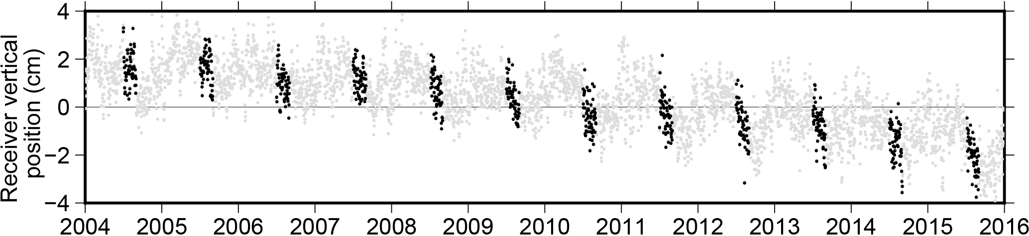
Figure 3 Time series of daily vertical positions of GPS receiver SG27, reflecting the solid earth movement (data source: http://geodesy.unr.edu/NGLStationPages/stations/SG27.sta). The mean has been removed. The black dots are from 1 July to 31 August. The rest are shown as gray dots. To simplify the figure, uncertainties of the receiver positions are not shown.

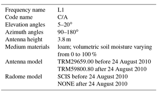
We first estimate the general varying pattern of the compositional height with changing soil moisture (in volumetric water contents, VWC) that increase from 0 to 100 % by an interval of 1 %. For organic-rich soils with a given VWC, we run the GPS multipath simulator of Nievinski and Larson (2014b), MPSImulator (publicly available at https://www.ngs.noaa.gov/gps-toolbox/MPsimul.htm), to simulate SNR data using the same settings as the real SNR data at SG27 (see Table 2 for a list of simulator settings). Then we apply the same GPS-IR data processing method as described earlier in Sect. 4.2 to calculate the compositional heights. Because of the changes of antenna and radome on 24 August 2010, we run the simulator using two antenna models and obtain two relationships of compositional heights versus soil moisture. Because the simulator does not include gain pattern models of the two antenna–radome combinations at SG27, we set the radome models as “SCIS” and “NONE” for the two cases, respectively. Next, we simulate a time series of compositional heights by using the soil moisture measured at U1-1.

5 Results

5.1 Changes of receiver position due to solid earth dynamics

Figure 3 shows the time series of V in the geocentric NA12 frame. The solid earth underwent regular cyclic vertical movements at the annual and semi-annual periods, due to surface mass loading from the atmosphere, ocean, and surface hydrology (van Dam et al., 1994, 2001), and a steady subsidence trend. The mean seasonal subsidence from 1 July to 31 August during 2004–2015 was 3.3 ± 0.2 cm. The best fit linear subsidence trend was 0.27 cm year⁻¹.

Table 2 Key settings used in MPSImulator. The others are set to the defaults.

5.2 Changes of surface elevation due to frozen ground dynamics

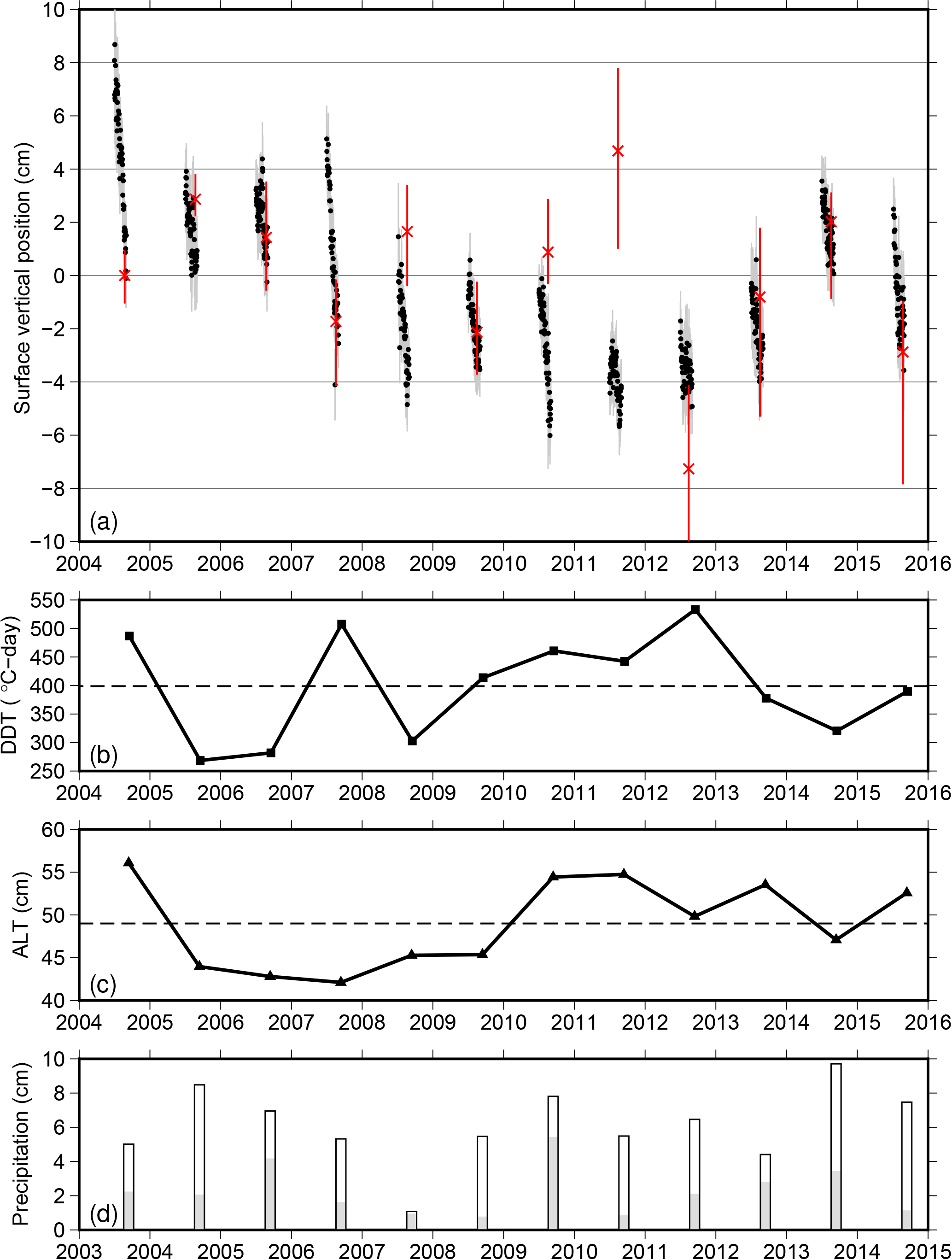
Figure 4 (a) De-meaned time series of surface vertical position. The black dots are the daily vertical positions of the reflecting surface at SG27, retrieved using GPS-IR. The error bars (standard error of the mean) are shown in gray. The red crosses are the vertical positions of ground measured annually in mid-August by Streletskiy et al. (2017), averaged over four sites at the CRREL grid, solid earth movement removed. The red bars show the range of elevation changes at the four sites. (b) Time series of the degree day of thawing (DDT) at the end of each thaw season. The dashed line denotes the 2004–2015 mean level. (c) Time series of active layer thickness (ALT) at SG27, scaled from the mean ALT measured at CALM grid. The dashed line denotes the 2004–2015 mean. (d) Cumulative precipitation during June–July–August (open bars) and August (gray bars), measured at the Barrow Airport. Note that the horizontal axis is shifted 1 year earlier from panel (a) to facilitate the comparison between the seasonal subsidence with precipitation in the previous summer (see more in Sect. 5.4).

Figure 4a shows the time series of surface elevation changes due to frozen ground dynamics from 2004 to 2015. We only present the values of S_F on snow-free days between 1 July and 31 August. The ground surface underwent gradual seasonal subsidence. Figure 4a also shows prominent interannual variability, which is associated with summer air temperatures. Using the DDT at the end of each thaw season as an indicator of warm/cool summers (Fig. 4b), we observe a general trend that larger seasonal subsidence occurred during warm summers such as 2004 and 2007 and smaller subsidence within cool summers such as 2005, 2006, and 2014. However, the subsidence was comparatively small during a warm summer in 2012, deviating from the general correlation. At secular scales, the ground surface underwent a steady subsidence of 1.05 ± 0.03 cm year⁻¹ from 2004 to 2010, followed by an uplift trend of 1.82 ± 0.06 cm year⁻¹ from 2011 to 2014, and then a subsidence from 2014 to 2015. The overall linear subsidence trend between 2004 and 2015 was 0.26 ± 0.02 cm year⁻¹.

5.3 Comparison between the GPS-IR and GPS campaign measurements

Our estimated surface elevation changes generally agree with the GPS campaign measurements of Streletskiy et al. (2017). Since the campaign measurements were conducted in late August, we can only compare these two in the interannual sense (Fig. 4a). Both sets of elevation change results are consistent within the uncertainties in individual years except 2008, 2010, 2011, and 2012. Both show similar subsidence trends between 2004 and 2010, and similar uplift trends during 2012–2014, and the subsidence from 2014 to 2015. After removing V, which has a linear subsidence trend of 0.27 cm year⁻¹, from the campaign measurements, we obtain an overall subsidence trend of 0.19 ± 0.14 cm year⁻¹ between 2004 and 2015. This is consistent with our GPS-IR trend of 0.26 ± 0.02 cm year⁻¹ within the uncertainties.

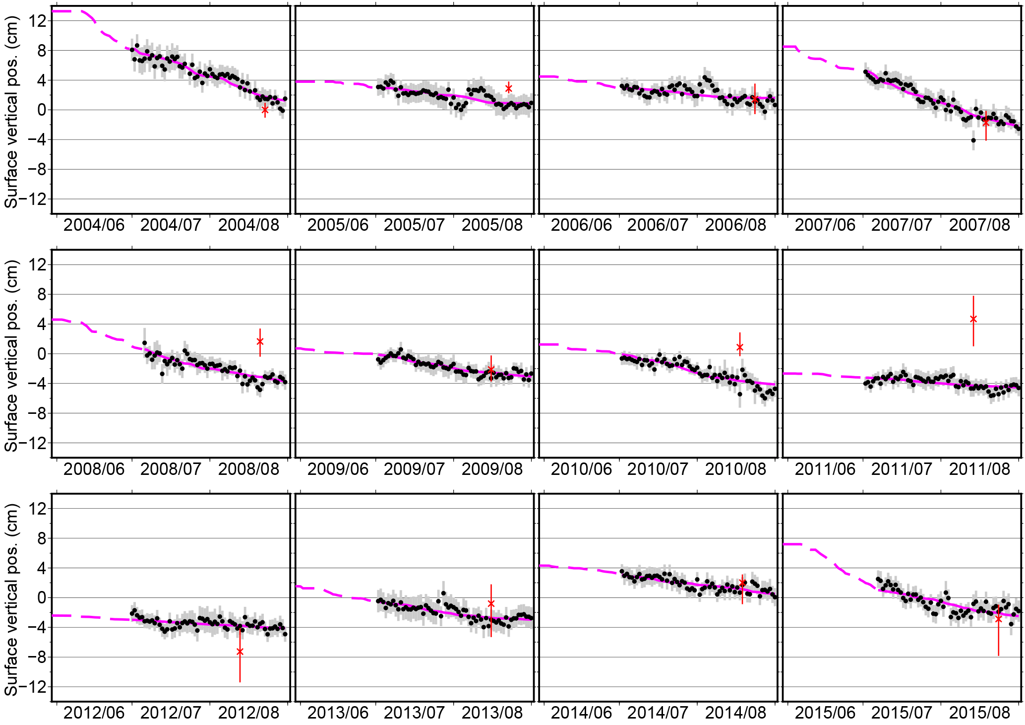
Figure 5 Similar to Fig. 4a, but showing the time series in each year from 2004 to 2015. The solid magenta lines are the best fit seasonal changes of surface elevation using Eq. (5). The dashed magenta lines denote the extended records back to 1 June.

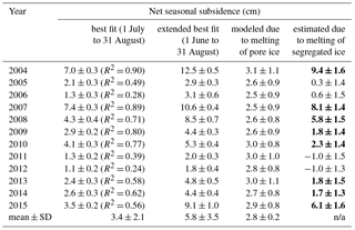
Table 3 Comparison among the best fit subsidence between 1 July and 31 August, extended best fit subsidence between 1 June and 31 August (i.e., entire thaw season), and the modeled maximum subsidence due to the melting of pore ice in the active layer. The R² values of the fit are listed in the parenthesis of the second column. The last column is the difference between the extended best fit and the modeled maximum subsidence, regarded as the net subsidence due to the melting of segregated ice. In the last column, the estimated subsidence values larger than the uncertainties are highlighted in bold. The last row lists the 12-year mean and the standard deviation (SD).

Out of the four mismatched years, the campaign measurements show strong heave relative to the previous August in three of them (i.e., heave from 2007 to 2008, from 2009 to 2010, from 2010 to 2011). Streletskiy et al. (2017) did not explicitly explain these observed heaves. The campaign measurements also show ∼ 13 cm of subsidence from August 2011 to August 2012, in contrast to the nearly zero changes between these two Augusts from our GPS-IR-based observations.

5.4 Comparison among the observed, best fit, and modeled seasonal subsidence

Year-by-year comparison shows that the simple square-root-of-DDT model (Eq. 5) generally fits the GPS-IR-retrieved elevation changes (Fig. 5). The R² values of the fitting ranging from 0.24 to 0.9 and a mean of 0.6 for all the years (Table 3). According to the best fit results, the net subsidence between 1 July and 31 August in each year ranged from 1.1 to 7.4 cm, with a 12-year mean of 3.4 cm and a standard deviation of 2.1 cm (the solid magenta lines in Fig. 5 and the second column of Table 3). Extending the best fit results to 1 June, we infer that the total subsidence within each thaw season ranged from 1.8 to 12.5 cm, with a 12-year mean of 5.8 cm and a standard deviation of 3.5 cm.

Our modeled subsidence due to the melting of pore ice spanning each thaw season (i.e., $d_{\mathrm{pore}}^{\max })$ was 2.8 cm on average, with small interannual variability. Such small variability is largely because the ALT varied little during the study period (Fig. 4c), which means that the total pore water volume in the active layer did not change much over the years. In terms of multiple-year average, the modeled seasonal subsidence is smaller than the best fit by 3.0 cm. Such residual is our estimated seasonal subsidence due to the melting of segregated ice (i.e., $d_{\mathrm{seg}}^{\max }$, listed in the last column of Table 3). The uncertainties of $d_{\mathrm{seg}}^{\max }$ are obtained by error propagation. In 8 out of 12 years, our inferred $d_{\mathrm{seg}}^{\max }$ are larger than their corresponding uncertainties, which will be used in the following analysis.

Since the subsidence caused by melting of segregated ice is controlled by the total amount of segregated ice in the active layer before thawing, we hypothesize that more segregated ice may develop after a wet thaw season, therefore resulting in larger subsidence during the following thaw season. Due to lack of soil moisture data throughout the study period, we use the cumulative precipitation in August as a proxy for excess soil water, which we refer to as the extra water that is more than a fully saturated active layer can hold before it starts to freeze. Figure 6 shows a scatter plot between $d_{\mathrm{seg}}^{\max }$ and the precipitation in the previous August. We observe two distinct groups: for $d_{\mathrm{seg}}^{\max }$ that are larger than 5 cm, they increase nearly linearly with the precipitation, which confirms our hypothesis; yet for small $d_{\mathrm{seg}}^{\max }$ (around 2 cm), they are independent of the precipitation.

5.5 Effects of soil moisture on the retrieved reflector height

Figure 7 shows the possible range of compositional height changes due to soil moisture changes from 0 to 100 %. The two curves correspond to the two antenna models, before and after the equipment change on 24 August 2010. Both curves show that reflector height increases monotonically with soil moisture. In the post-2010 case, the reflector height shows a higher sensitivity to soil moisture than the pre-2010 case.

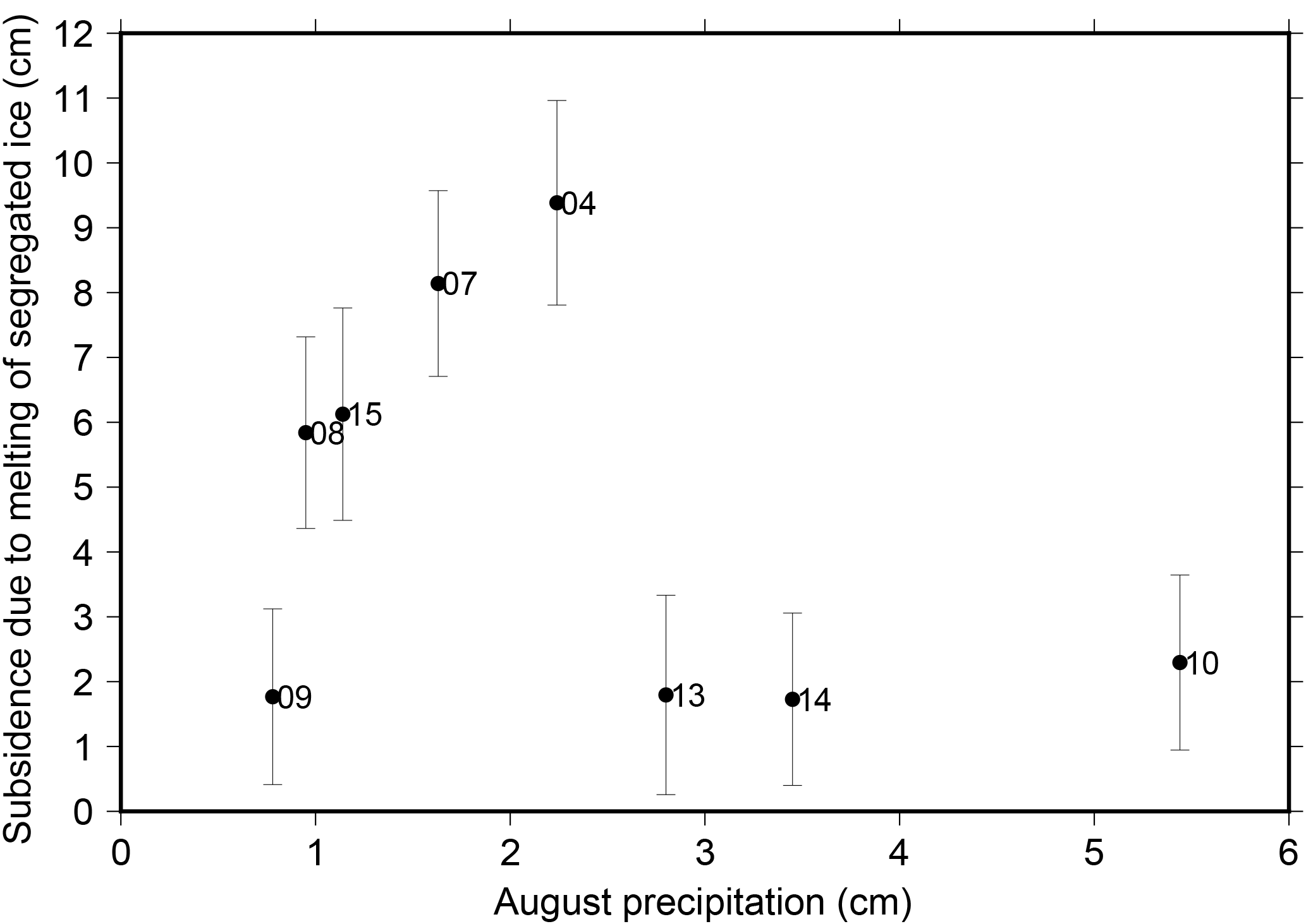
Figure 6 Scatter plot between the estimated subsidence due to the melting of segregated ice in the active layer and the precipitation in the previous August. The labels refer to the year of the subsidence.

Figure 7 Changes of compositional height (i.e., apparent reflector height) with soil moisture based on the simulated SNR data using two antenna models: TRM29659.00 was used before 2010 Aug 24; TRM59800.80 was used after 2010 Aug 24.

Figure 8a shows the time series of VWC at 5 cm depth, measured at U1-1. Five centimeters is the resolved depth range for soil moisture retrievals using GPS-IR (Larson et al., 2008). Between July and August in each year, the change range of VWC was up to 15 %. The only exception was 2009 when the range was the largest, ∼ 25 %. In many summers, the soil moisture first decreased from June to July, then increased in August. Rainfall events sharply increased the soil moisture (e.g., in 2010 and 2011).

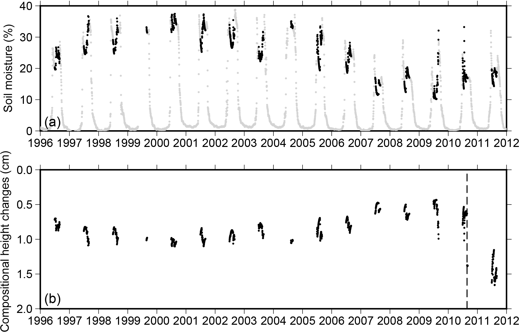
Figure 8 (a) Daily soil moisture at 5 cm depth, measured at the CALM Barrow soil–climate site U1-1. Black dots and gray dots denote records during July–August and in other months, respectively. The records have data gaps in the summers of 2000 and 2004. (b) The simulated changes of compositional height in July and August. Because an increase in compositional height can be potentially mistakenly interpreted as an apparent ground surface subsidence, the vertical axis of this figure is flipped to facilitate comparison with subsidence plots such as Fig. 4a. The vertical dashed line denotes the date of antenna change (i.e., 24 August 2010).

Figure 8b shows the time series of the simulated composition height changes. Because the soil moisture records are not from within the GPS-IR footprint and their period does not fully overlap with our GPS-IR records, we cannot use the simulated compositional heights to “correct” the GPS-IR reflector height results. Instead, we interpret the simulated results to assess the possible effects of soil moisture, in the following aspects. First, in our case using the settings listed in Table 2, the compositional heights are always positive. However, because we are only interested in temporal changes, any systematic bias due to soil moisture changes is irrelevant. Second, the changes of compositional height within each summer were within in 0.5 cm, much smaller than the reflector height changes at seasonal scales. Third, the largest interannual change in compositional height was between 2010 and 2011, due to the antenna change. For instance, the compositional height increased by ∼ 0.8 cm between 1 July 2010 and 1 July 2011. This is still smaller than the ∼ 3.2 cm subsidence based on the GPS-IR reflector height records. Fourth, because the near-surface soil moisture in Barrow did not undergo any significant decadal changes, the secular trend of compositional height was negligible (e.g., $\mathrm{1.4}\times {\mathrm{10}}^{-\mathrm{5}}$ cm year⁻¹ for 1996–2011). For the above reasons, we conclude that our retrieved changes of ground surface elevation are not significantly affected by these soil moisture effects.

6 Discussion

6.1 Thawing/freezing of the transition layer as a mechanism for sub-decadal subsidence/uplift

We postulate that both large seasonal subsidence and the decadal subsidence trend are due to thawing of the transition layer in warm summers. Figure 4a shows that the largest seasonal surface subsidence occurred in 2004 and 2007, which were the warmest summers during the 12 years (Fig. 4b). The thaw indices also increased from 2005 to 2013 with a trend of 20.3 ^∘C days year⁻¹, which may cause the gradual thawing of the transition layer and thus the linear surface subsidence trend during the same period. In years when excess water remains in the active layer before freezing, significant accretions of segregated ice can develop within the transition layer and cause surface heave during winter (Fig. 6).

The transition layer is widely thought to act as a buffer between the thawing of the active layer and ice-rich permafrost in that it protects the permafrost beneath from thawing (Hinkel and Nelson, 2003; Shur et al., 2005). The progressive thawing of the transition layer causes a gradual surface subsidence that is barely observable without accurate measurements over decades. In addition to the GPS campaigns conducted by Shiklomanov et al. (2013) and Streletskiy et al. (2017), as well as the InSAR study of Liu et al. (2010) over Prudhoe Bay, our GPS-IR results provide another set of observations of such subtle decadal changes on the North Slope of Alaska. The two independent estimates of linear trends at Barrow agree well (i.e., 0.26 ± 0.02 cm year⁻¹ from this work and 0.19 ± 0.14 cm year⁻¹ from the GPS campaigns of Shiklomanov et al., 2013). The InSAR measurements of Liu et al. (2010) revealed linear subsidence trends of 0.1 to 0.4 cm year⁻¹ between 1992 and 2002 over Prudhoe Bay, consistent with the two Barrow studies within the same order of magnitude.

6.2 Merits and limitations of long-lasting, daily GPS-IR measurements for frozen ground studies

The surface elevation changes retrieved from our GPS-IR measurements are daily and long-lasting, which are unique and valuable for quantifying subtle surface changes over permafrost areas. In cases of no major instrumental changes or when any vertical shift in GPS antenna phase center due to instrument change is known (e.g., 2 mm in 2010 for SG27), the GPS-IR-based measurements are consistent, sustained, and progressively increasing. This is important for studying seasonal, interannual, and long-term dynamics of the active layer and permafrost. In situ ALT or GPS campaign measurements were typically conducted annually, but not always on the same day of the year due to logistical constraints. Our GPS-IR results show that the seasonal changes are more significant than the interannual and long-term changes. It is possible that the interannual and long-term changes estimated from a poorly sampled record of elevation changes (e.g., annual measurements) may be aliased by the seasonal changes (Liu et al., 2015). Our daily sampled and long-lasting records from GPS-IR can avoid such aliasing problem and give robust estimates on the interannual and long-term variations.

Since the GPS-IR-estimated reflector height directly reflects the frozen ground dynamics, it is unnecessary to process geodetic-level GPS positioning data or correcting for the solid earth movement. Knowing the GPS receiver position, nonetheless, we can obtain the “absolute” surface ground elevation changes in a geocentric frame (i.e., the S term in Fig. 2). These types of geocentric records can be directly compared with altimetry observations and be used to tie locally reference measurements, such as InSAR. For instance, the surface elevation changes we have obtained at SG27 would serve as a good reference point to tie InSAR measurements to the geocentric Earth frame. The daily records would also complement InSAR measurements by filling their temporal gaps.

However, GPS-IR suffers from a few limitations. First, the day-to-day variations in our retrieved reflector height are unreliable, due to relatively large uncertainties (centimeter level in the case of SG27) and the soil moisture effects. Therefore, we choose not to interpret the daily changes in our time series as associated with frozen ground dynamics. Second, GPS-IR signals on snow-covered days are dominated by snow depth changes, limiting the use of this type of data for studying ground surface changes only on snow-free days. Nonetheless, as we have demonstrated in this study, noisy daily records continuously spanning 60 days in each summer and 12 years can provide robust estimates of seasonal, interannual, and decadal changes. Third, similar to typical in situ observations, GPS-IR only offers site-specific measurements. We note that the GPS-IR method takes spatial averages within the reflection footprint (∼ 90 m radius in the case of SG27). This averaging helps to mitigate the spatial heterogeneities due to changes in soil and vegetation, as well as active layer and ground ice conditions. Lastly, reliable GPS-IR retrieval requires a smooth surface within the footprint. Therefore, this method is not applicable for studying thermokarst landforms.

7 Conclusions

Using a continuously operating station mounted deep into permafrost in Barrow, we show that the reflector height retrieved using GPS-IR can estimate surface elevation changes during thaw seasons at a daily interval. This 12-year-long record offers quantitative insights into the seasonal, interannual, and decadal variabilities of the flat terrain in continuous permafrost. Such continuous, consistent, and daily records spanning a long time period are of great value to monitoring permafrost changes in a changing climate. The GPS-IR data can also help to fill in the temporal gaps in other field-based or remote sensing methods, and tie relative measurements, such as InSAR, to the geocentric frame.

This method could be potentially extended to numerous continuously operating global navigation satellite system (GNSS) receivers in cold regions (more than 200 sites are located in permafrost areas in the Northern Hemisphere). Our study also highlights the importance of long-lasting surface elevation changes and in situ soil measurements (such as active layer thickness and soil moisture), ideally at the same location, for a comprehensive and quantitative understanding of near-surface dynamics of the active layer and permafrost.