the Creative Commons Attribution 4.0 License.
the Creative Commons Attribution 4.0 License.
 | 07 Dec 2018
Sensitivity of the current Antarctic surface mass balance to sea surface conditions using MAR
Charles Amory
Cécile Agosta
Alison Delhasse
Sébastien Doutreloup
Pierre-Vincent Huot
Coraline Wyard
Thierry Fichefet
Xavier Fettweis
Estimates for the recent period and projections of the Antarctic surface mass balance (SMB) often rely on high-resolution polar-oriented regional climate models (RCMs). However, RCMs require large-scale boundary forcing fields prescribed by reanalyses or general circulation models (GCMs). Since the recent variability of sea surface conditions (SSCs, namely sea ice concentration, SIC, and sea surface temperature, SST) over the Southern Ocean is not reproduced by most GCMs from the 5th phase of the Coupled Model Intercomparison Project (CMIP5), RCMs are then subject to potential biases. We investigate here the direct sensitivity of the Antarctic SMB to SSC perturbations around the Antarctic. With the RCM “Modèle Atmosphérique Régional” (MAR), different sensitivity experiments are performed over 1979–2015 by modifying the ERA-Interim SSCs with (i) homogeneous perturbations and (ii) mean anomalies estimated from all CMIP5 models and two extreme ones, while atmospheric lateral boundary conditions remained unchanged. Results show increased (decreased) precipitation due to perturbations inducing warmer, i.e. higher SST and lower SIC (colder, i.e. lower SST and higher SIC), SSCs than ERA-Interim, significantly affecting the SMB of coastal areas, as precipitation is mainly related to cyclones that do not penetrate far into the continent. At the continental scale, significant SMB anomalies (i.e greater than the interannual variability) are found for the largest combined SST/SIC perturbations. This is notably due to moisture anomalies above the ocean, reaching sufficiently high atmospheric levels to influence accumulation rates further inland. Sensitivity experiments with warmer SSCs based on the CMIP5 biases reveal integrated SMB anomalies (+5 % to +13 %) over the present climate (1979–2015) in the lower range of the SMB increase projected for the end of the 21st century.
- Article
(1123 KB) - Full-text XML
-
Supplement
(4974 KB) - BibTeX
- EndNote


Sea ice concentration (SIC) and sea surface temperature (SST), hereafter referred to as sea surface conditions (SSCs), influence the exchange of gas, momentum, and heat at the air–sea interface at high latitudes. Due to its high albedo and thermal insulation, sea ice notably affects the thermodynamic and radiative properties of the ocean surface. Sea ice also prevents evaporation and inherent water vapour loading of air masses, potentially affecting precipitation at high latitudes. This is of particular importance for the Antarctic ice sheet (AIS) as its surface mass balance (SMB) is mainly controlled by precipitation (Agosta et al., 2018; van Wessem et al., 2018).
Southern Ocean SSCs and especially sea ice extent (generally defined as the area of all grid cells of satellite or model products with a SIC of at least 15 %) have experienced a significant increase since the 1970s (Massonnet et al., 2013; Parkinson and Cavalieri, 2012), highly contrasting with the dramatic decline reported in the Arctic Ocean (Cavalieri and Parkinson, 2012). Nonetheless, this general trend conceals major regional differences. For instance, the Amundsen–Bellingshausen seas showed a strong decrease in sea ice extent, unlike other surrounding Antarctic seas (Turner et al., 2016). Despite the observed changes in the Antarctic SSCs and their large potential impacts on the climate system, the Antarctic SMB did not exhibit any significant trend at the continental scale over the last decades (Agosta et al., 2018; Bromwich et al., 2011; Favier et al., 2017; Frezzotti et al., 2013; Lenaerts et al., 2012).
Several modelling studies have illustrated the influence of open-ocean areas on the AIS climate, for instance through a strong atmospheric heating (Gallée, 1995; Simmonds and Budd, 1991), an enhancement of cyclone activity (Gallée, 1996; Krinner et al., 2014; Simmonds and Wu, 1993), and intensified precipitation related to intensified evaporation (Bromwich et al., 1998; Weatherly, 2004; Wu et al., 1996). Conversely, the atmosphere has been shown to be less sensitive to SIC anomalies than SIC to atmosphere anomalies (Bailey and Lynch, 2000; Simmonds and Jacka, 1995) as anomalies induced by the ocean surface are often restricted to the lower atmospheric layers above the Southern Ocean (Van Lipzig et al., 2002). However, these previous studies were based on coarse-resolution models (Weatherly, 2004), with simplified physics, resulting notably in biased surface sublimation (Noone and Simmonds, 2004), or on regional climate models (RCMs), forced by earlier and less reliable reanalyses and over short periods (Van Lipzig et al., 2002).
High-resolution polar-oriented RCMs provide more reliable estimates of the Antarctic SMB components, but they depend on their forcing boundary conditions, including SSCs. Using adequate SSCs in climate models could be as crucial as using a suitable downscaling model (Beaumet et al., 2017; Krinner et al., 2008). This is of particular importance since most general circulation models (GCMs) from the 5th phase of the Coupled Model Intercomparison Project (Taylor et al., 2012) have failed to reproduce the SSC temporal and spatial variability in the Southern Ocean area over the last decades (Agosta et al., 2015; Mahlstein et al., 2013; Roach et al., 2018; Shu et al., 2015; Turner et al., 2013). As the projected Antarctic SMB could highly depend on the representation of the present sea ice extent (Agosta et al., 2015), we investigate here the sensitivity of the Antarctic SMB to SSCs and more specifically to CMIP5 SSC anomalies with the “Modèle Atmosphérique Régional” (MAR) for the period 1979–2015. This will help in the partitioning of the uncertainty in Antarctic SMB projections resulting from biased SSCs in GCMs from the uncertainty resulting from biased large-scale circulation patterns. Even though MAR is a well adapted tool to study the climate sensitivity to SSCs (Gallée, 1995, 1996; Messager et al., 2004; Noël et al., 2014), this study only discusses the direct and local impact of SSCs on the Antarctic SMB. This means that no feedbacks on the general circulation associated with sea ice removal are considered (Bromwich et al., 1998; Krinner et al., 2014). Only direct impacts on air temperature, moisture, and SMB components are accounted for. Note that the general atmospheric circulation remains unchanged in our sensitivity experiments.
A description of MAR, the model set-up, and sensitivity experiments is given in Sect. 2. Section 3 presents model evaluation, as well as the observations and methods used for comparison. The influence of SSCs on the Antarctic SMB is analysed in Sect. 4, while we discuss the direct impacts of perturbed SSCs in Sect. 5. Our main conclusions are summarized in Sect. 6.
2.1 The MAR model
The ability of the regional climate model MAR to reproduce the climate specificities of polar regions has been extensively evaluated (Agosta et al., 2018; Amory et al., 2015; Fettweis et al., 2017; Gallée et al., 2015; Lang et al., 2015). MAR is a hydrostatic, primitive equation atmospheric model (Gallée and Schayes, 1994), which includes a cloud microphysics module solving conservation equations for specific humidity, cloud droplets, rain drops, cloud ice crystals, and snow particles (Gallée, 1995). The effect of sea spray on heat fluxes or on water vapour concentration is parameterized following Andreas (2004). The atmospheric model is coupled to the 1-D SISVAT (De Ridder and Gallée, 1998) module, which consists of soil and vegetation (De Ridder and Schayes, 1997), snow (Gallée and Duynkerke, 1997; Gallée et al., 2001), and ice (Lefebre et al., 2003) submodules that simulate energy and mass fluxes between the surface and the atmosphere. The snow–ice module includes submodules for surface albedo, meltwater refreezing, and snow metamorphism based on the CROCUS model (Brun et al., 1992). Regarding interactions between the atmosphere and the ocean, SISVAT considers distinct sea ice and open-water sub-grid cells. Open-ocean roughness length for momentum and heat follows Wang (2001), while the momentum roughness length over snow surfaces (sea ice and ice sheet grid cells) is computed as a function of air temperature as proposed in Amory et al. (2017). Fluxes and roughness lengths are separately calculated over sea ice and water, and are afterward weighted according to sea ice and open-ocean fractions (Gallée, 1996). In this study, we use MAR version 3.6.4, recently adapted to Antarctica (Agosta et al., 2018). Although MAR includes a drifting snow module (Gallée et al., 2001), this module has been switched off similarly to Agosta et al. (2018) as the new version of this module is still under evaluation against satellite and ground-based observations.
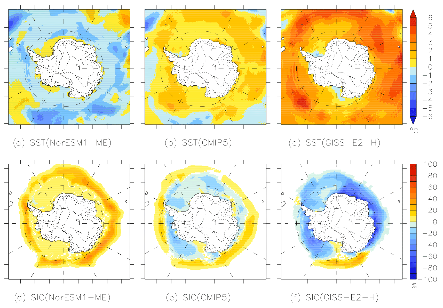
Figure 1Top: SST anomalies (∘C) of (a) NorESM1-ME, (b) CMIP5 average, and (c) GISS-E2 compared to ERA-Interim SST over 1979–2005. Bottom: SIC anomalies (%) for (d) NorESM1-ME, (e) CMIP5 average, and (f) GISS-E2 compared to ERA-Interim SIC over 1979–2005. These anomalies were introduced in the 6-hourly ERA-Interim SSCs.
2.2 Set-up
As the ERA-Interim reanalysis (Dee et al., 2011) is considered as one of the most reliable reanalyses for the Antarctic region (Agosta et al., 2015; Bracegirdle and Marshall, 2012; Bromwich et al., 2011), MAR is forced by ERA-Interim every 6 h over 1979–2015 at its atmospheric lateral boundaries (pressure, wind, specific humidity, and temperature) and over the ocean surface (SIC and SST). It is worth noting that ERA-Interim uses the SST and SIC values from ERA-40, which are based on monthly and weekly ocean forcing fields (Fiorino, 2004), until January 2002. Afterwards, a switch was made with the daily operational NCEP product and since 2009 with the Operational SST and Sea Ice Analysis (OSTIA). The latter is a daily global SST analysis product at a 0.05∘ resolution (Donlon et al., 2012; Stark et al., 2007). For each grid cell with a ERA-Interim SIC value greater than 0 %, the MAR sea ice thickness is initially fixed at 55 cm and sea ice can be covered by snow. The sea ice thickness can then evolve as a function of accumulated snowfall or surface snowmelt or ice melt, with a minimum thickness of 10 cm as long as the ERA-Interim SIC is positive. The sub-grid cells' SST beneath sea ice is fixed at −2 ∘C in the MAR snow model, while the sea ice surface temperature is free to evolve according to its surface energy balance. Finally, as for spin-up time, we start our simulations in March 1976 using ERA-40 reanalysis (Uppala et al., 2005) until 1979 with initial snowpack conditions interpolated from a previous reference simulation (Agosta et al., 2018).
Compared to Agosta et al. (2018), our integration domain (Fig. 1a) has been extended to include the maximum seasonal sea ice extent as well as the major moisture source for precipitation over the AIS (Sodemann and Stohl, 2009). A resolution of 50 km has been selected to preserve a reasonable computational time. The Antarctic topography is based on the 1 km resolution digital elevation model Bedmap2 from Fretwell et al. (2013). An upper-air relaxation extending from the top of the atmosphere to 6 km above the surface is used in order to constrain the MAR general atmospheric circulation (Agosta et al., 2018; van de Berg and Medley, 2016). This upper relaxation prevents potential feedbacks between the ocean state and the general atmospheric circulation. Similarly to Noël et al. (2014), the SMB sensitivity to SSC perturbations will thus be limited to the direct and local impacts of SST and SIC anomalies within the MAR integration domain.
2.3 Simulations
In this study, we consider MAR forced by ERA-Interim over 1979–2015 as the reference simulation. We perform two sets of sensitivity experiments in which SSCs from ERA-Interim are perturbed as described below. The first set follows the methods described in Noël et al. (2014), which are simplified and idealized scenarios, while in the second set, SSCs are modified according to SSC anomalies from CMIP5 models. In both cases, we analyse the direct impact of SSC anomalies on the Antarctic SMB.
2.3.1 SST sensitivity experiments
In these experiments, the 6-hourly ERA-Interim SST are decreased (increased) by 2 ∘C (SST ± 2) and 4 ∘C (SST ± 4) for ice-free grid cells. In cases of an SST reduction, ice-free oceanic grid cells are converted into full ice-covered grid cells if the SST drops below the assumed seawater freezing point (−2 ∘C). For an SST increase, the SST of any grid cell with a positive SIC value is set to the melting point (0 ∘C) to avoid positive SST and to prevent any SIC change.
2.3.2 SIC sensitivity experiments
To prevent changes at the interface between ice-covered and ice-free grid cells that are too strong, ERA-Interim SIC are reduced (increased) by the minimum (maximum) SIC value of the three and six ocean neighbours of each MAR grid cell. These experiments are called SIC ± 3 and SIC ± 6. Knowing that the resolution is 50 km, this means that the SIC is gradually decreased (increased) by a distance of 150 and 300 km. Following Noël et al. (2014), a SST correction is applied in order to prevent open-water temperature from dropping below −2 ∘C and maintain the SST of sea ice-covered grid cells below the melting point (0 ∘C).
2.3.3 Combined SST/SIC sensitivity experiments
Combined SST/SIC forcing fields are computed according to the two previous subsections. The added value of these experiments is the simultaneous representation of the increase (decrease) in sea ice extent associated with the decrease (increase) in SST. They are named SST , SST .
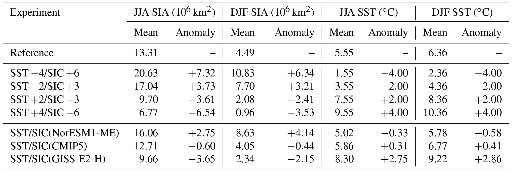
Table 1JJA and DJF sea ice area (SIA) (106 km2) within the MAR domain over the period 1979–2015. SIA is defined as the sum of the products of the SIC and the area of all grid cells with a SIC value of at least 15 %. The DJF (JJA) seasonal mean SST is computed for the ocean free of ice in all experiments in DJF (JJA). We only considered grid cells remaining free of ice (SIC <15 %) in all experiments in order to remove the influence of sea ice on surface temperature and numerical artefacts due to differences in open-ocean areas.
2.3.4 CMIP5-based sensitivity experiments
In addition to the spatially homogeneous perturbations described above, we evaluate how SSC anomalies from CMIP5 models over the current climate can influence the present-day Antarctic SMB modelled by RCMs. For that purpose, we have determined a perturbation whose magnitude is representative of the CMIP5 ensemble bias. Firstly, monthly SSCs over 1979–2005 from all the CMIP5 models (using the historical scenario), as well as from ERA-Interim, were interpolated on the MAR grid (50 km×50 km) using an inverse-distance weighted method based on the four CMIP5 models/ERA-Interim grid cells nearest to the current MAR one. We then computed the CMIP5 ensemble average from the interpolated CMIP5 monthly SSCs. Monthly SST anomalies between CMIP5 and ERA-Interim were computed only if the SICs from both the CMIP5 ensemble average and ERA-Interim were less than 50 % to avoid introducing additional temperature biases. Secondly, we averaged the monthly anomalies to obtain a mean anomaly, supposed to represent a constant bias over time.
New 6-hourly forcing SST are calculated as the sum of the 6-hourly ERA-Interim (i.e. for a specific day of a certain month) and the corresponding monthly anomaly in SST from the CMIP5 ensemble average (Fig. 1b), hereafter referred to as the SST(CMIP5) experiment. In the same way, we define SIC(CMIP5) experiments in which SIC anomalies (Fig. 1e) from the CMIP5 ensemble average are added to the 6-hourly ERA-Interim SIC. Introducing CMIP5 anomalies into the original ERA-Interim SSCs enables constant CMIP5 anomalies to be accounted for with the seasonal and interannual SSC variability represented in the ERA-Interim reanalysis. The combined SST/SIC anomaly experiment is performed by adding CMIP5-averaged SST and SIC anomalies to ERA-Interim and is hereafter referred to as SST/SIC(CMIP5). Following the same method, we perform combined experiments for two selected CMIP5 models, namely NorESM1-ME (Bentsen et al., 2013) and GISS-E2-H (Schmidt et al., 2014), respectively representative of colder (i.e. lower SST and higher SIC) and warmer (i.e higher SST and lower SIC) SSCs than ERA-Interim as shown in Agosta et al. (2015). These experiments are hereafter called SST/SIC(NorESM1-ME) (Fig. 1a, d) and SST/SIC(GISS-E2-H) (Fig. 1c, f).
Table 1 compares SSC perturbations to the reference SSCs for June–July–August (JJA) and December–January–February (DJF) SST and sea ice area (SIA). The mean SST and SIC anomalies of the CMIP5 ensemble average, NorESM1-ME, and GISS-E2-H are also listed. The SIA is defined as the sum of the products of the SIC and the area of all grid cells with a SIC value of at least 15 %. SIA is preferred to sea ice extent because it better accounts for SIC variations (Roach et al., 2018). Sensitivity experiments with perturbed SST by ±2 ∘C and SIC with the ±3 neighbour grid cells are 1.5 times as large as CMIP5 mean anomalies over the current climate. However, it should be remembered that our sensitivity experiments are not based on climatologically consistent SIC (SST) perturbations related to SST (SIC) perturbations. For instance, the SIC prescribed in our experiments associated with 2 ∘C warmer SST could be significantly different from the real SIC in a 2 ∘C warmer climate since we do not use SIC projections from a GCM.
Since the MAR SMB has already been evaluated against the GLACIOCLIM-SAMBA dataset (Favier et al., 2013) over the AIS at 35 km resolution by Agosta et al. (2018), only a brief evaluation is proposed here to highlight the influence of using a coarser horizontal resolution on the SMB representation. We follow the same method as in Agosta et al. (2018).
Modelled values are interpolated to the observation locations using a four-nearest inverse-distance-weighted method. Only SMB observations after 1950 are considered. Concerning observations collected before our study period (1979–2015), the mean 1979–2015 modelled SMB values are compared to observations covering more than 8 years. For SMB observations beginning after 1979, modelled SMB values are compared to SMB observations in the same period. This procedure removed 206 observations from the GLACIOCLIM-SAMBA dataset. Then, all remaining observations located in the same MAR grid cell are averaged, and so the modelled SMB values are previously interpolated to the observation locations. Finally, as snow accumulation exhibits a very high variability at the kilometre scale (Agosta et al., 2012), unresolved at 50 km resolution, we restrain our comparison to grid cells containing more than one observation, i.e. 205 averaged comparison pairs. The comparison without the minimum observation number criterion per grid cell (462 points) is available in the Supplement (Fig. S1).
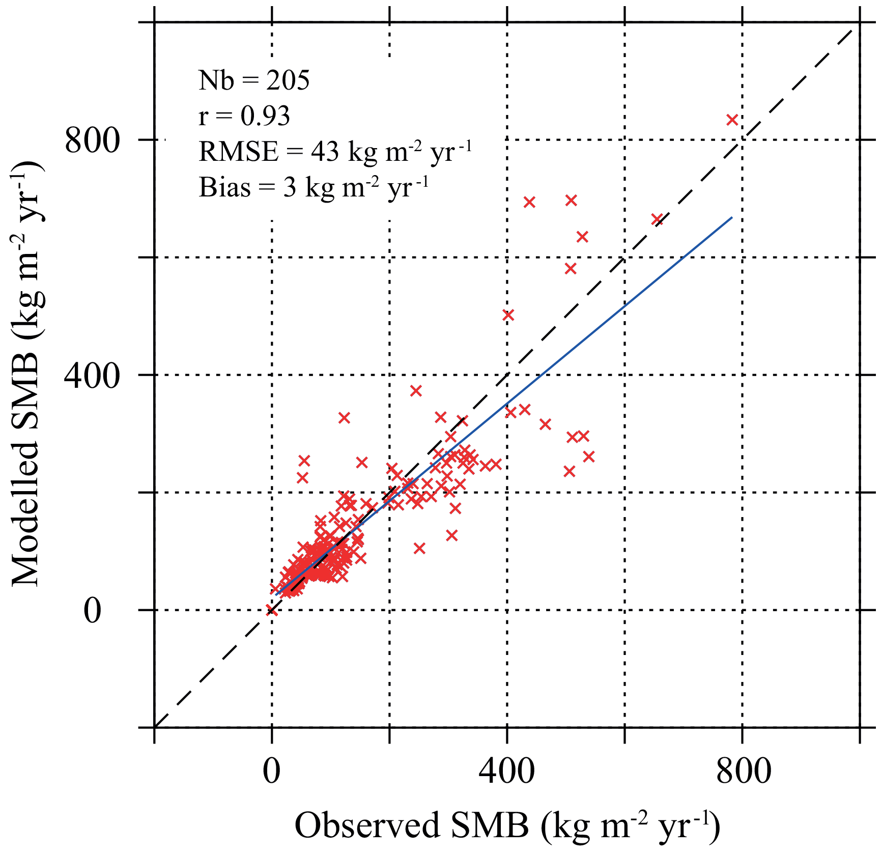
Figure 2Comparison between MAR SMB and observed SMB from the GLACIOCLIM-SAMBA database (Favier et al., 2013) for 1950–2015. Bias and RMSE units are kg m−2 yr−1. The averaged observation mean is 65 kg m−2 yr−1.
The high value of the correlation coefficient (r=0.93) between observed and modelled SMB values shows that MAR correctly represents the Antarctic SMB spatial variability at 50 km resolution over the 1979–2015 period (Fig. 2). Except over Dronning Maud Land, the margins of the Amery Ice Shelf, and a transect in Wilkes Land, MAR overestimates the SMB (locally up to a factor of 5, Fig. S2).
As also shown by Franco et al. (2012) over the Greenland ice sheet, these biases could partially arise from the coarse resolution used here (50 km), which induces a significantly smoothed topography at the ice sheet margins. This leads to an unsatisfactory representation of the topographic barrier effect, allowing the precipitation systems modelled by MAR to penetrate too far inland.
In order to estimate the biases and the uncertainty related to our resolution, the reference SMB of this study was briefly compared to the SMB at 35 km resolution from Agosta et al. (2018) (Fig. S3). This comparison also shows an SMB overestimation in the reference run compared to SMB results at a higher resolution, although this overestimation appears to be non-significant relative to the modelled interannual variability. The largest anomalies can be found over the Antarctic Peninsula and areas with a high spatial variability in orography such as the Transantarctic Mountains. The coarse 50 km resolution used here leads to artificially overestimated precipitation on the windward sides of orographic barriers. This is notably the case over the Filchner-Ronne and Ross ice shelves, where the Amundsen Sea Low generates a return flow. However, it should be noted that the SMB anomalies of our 50 km reference run compared to both 35 km results (Agosta et al., 2018) and observations are smaller than the SMB anomalies due to SSC perturbations presented in Sect. 4.
In this section, we analyse the local and direct impact of SSC anomalies on the Antarctic SMB and its components modelled by MAR forced by ERA-Interim over 1979–2015 (maps of SMB components for all experiments can be found in Figs. S4–S8). Since liquid precipitation accounts for negligible mass gains compared to snowfall (Table S1 in the Supplement), we do not distinctly analyse snowfall and rainfall over the AIS. As the large majority of surface meltwater and rainfall percolates and refreezes into the snowpack, runoff is a negligible component of the Antarctic SMB in both the reference and sensitivity experiments. However, some runoff events can occur on the Antarctic Peninsula (AP) and are enhanced in sensitivity experiments with warmer SSCs (+2 Gt yr−1 in SST/SIC(GISS-E2-H) and +6 Gt yr−1 in SST +4/SIC −6). The AP is characterized by a sharp elevation gradient inadequately resolved at 50 km resolution, leading to a poor representation of specific climatic processes encountered in complex topography such as the Foehn effect. Elsewhere coastal runoff amounts stand for very low values. Due to the coarse model resolution limiting the representation of the atmosphere dynamics over the AP and the marginal contribution of runoff to surface mass loss compared to sublimation, surface meltwater production is discussed hereafter instead of runoff amounts. This allows possible areas to be located where the occurrence of surface melting could possibly affect the surface climate through an increase in snowpack cohesion inhibiting wind erosion (Li and Pomeroy, 1997), or the ice sheet dynamics through meltwater percolation and subsequent ice shelf destabilization (Bevan et al., 2017).
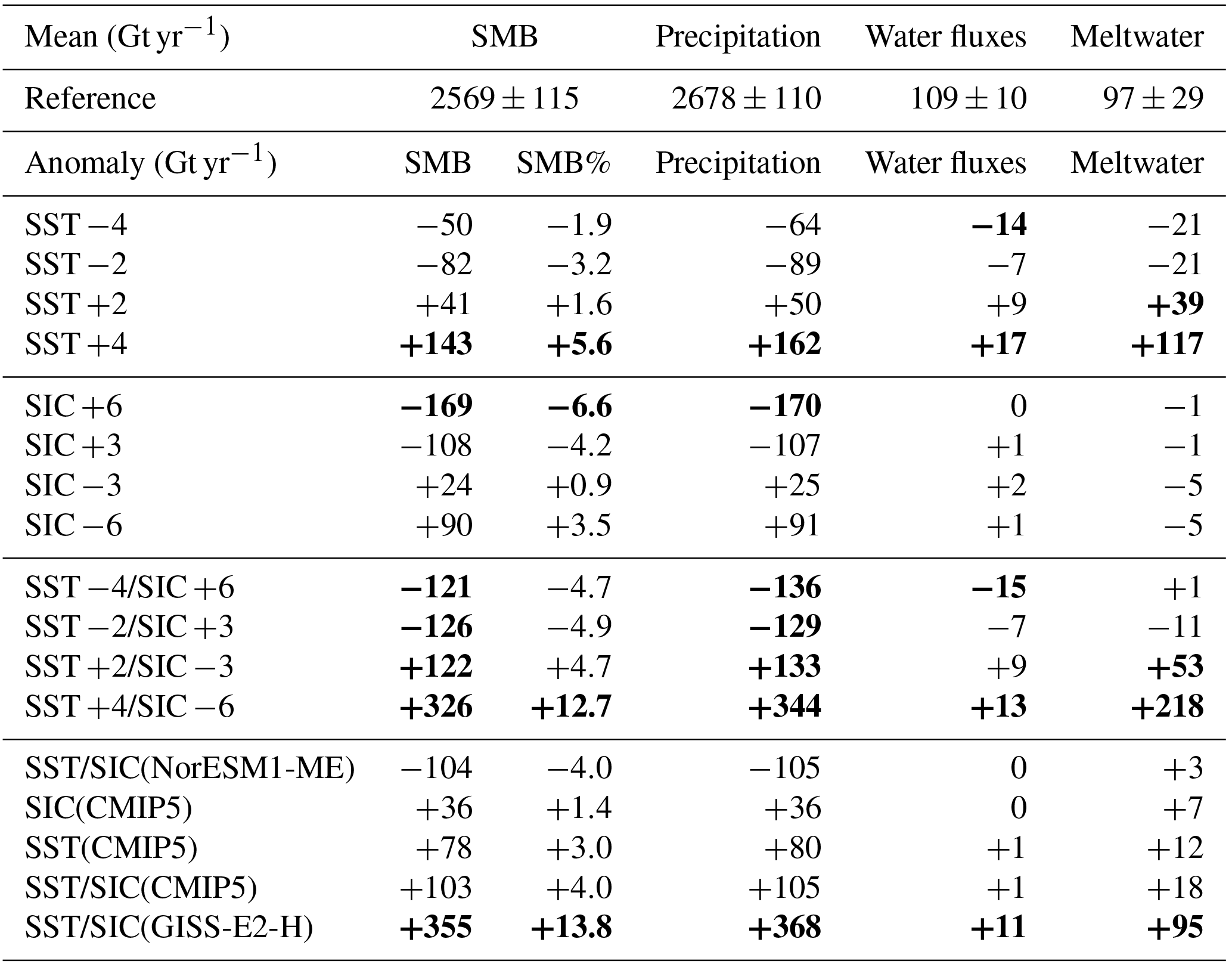
Table 2Top: annual mean integrated (Gt yr−1) and standard deviation (Gt yr−1) SMB, precipitation, water fluxes (sublimation and deposition processes), and surface meltwater production over the whole AIS (including grounded and floating ice) for the reference run (1979–2015). Positive water fluxes represent a mass loss through sublimation and evaporation while negative water fluxes are representative of deposition processes. Bottom: Difference of annual mean integrated SMB (Gt yr−1 and %), its components, and meltwater (Gt yr−1) between each sensitivity test and the reference simulation (1979–2015). Anomalies larger than the interannual variability are considered as significant and are displayed in bold.
4.1 Sensitivity to SST perturbations
The higher evaporation and inherent increase in air moisture content in SST +2 and SST +4 experiments induce significantly stronger precipitation rates (i.e. greater than the interannual variability) in coastal areas. Figure 3a points out an opposite pattern between AIS coastal and central areas with a decrease in precipitation over the plateau and large ice shelves (Filchner-Ronne, Ross, and Amery). The warmer ocean leads to an increase in near-surface air temperature of the same magnitude as the increase in SST converts snowfall into rainfall over the ocean (Figs. S5a, m and S6a, m). Higher air temperature also causes a significant increase in surface melt, twice as large as for SST +4 relative to the reference simulation (Fig. S8a). However, melt and rainfall water can percolate into the snowpack, which remains unsaturated except in a few places. As a consequence, the surface albedo remains high and does not strengthen melting. Even if mass losses due to surface sublimation are larger in SST +4 (Fig. S7a and Table 2) because of higher air temperature, increased precipitation dominates and the SMB anomaly is significantly positive (Table 2 and Fig. 3a).
Conversely, a reduction of the SST leads to non-significant negative integrated SMB anomalies (Table 2). Lower SST weaken evaporation at the ocean surface and reduce the saturation water vapour pressure, resulting in smaller annual mean integrated precipitation over the whole AIS. This decrease in precipitation mainly explains local negative SMB anomalies in coastal areas (e.g. Victoria Land, Wilkes Land, Drauning Maud Land, Ellsworth Land, and Marie Byrd Land; Fig. 3e, p; Fig. S9 locates these coastal areas). However, precipitation over large ice shelves is slightly enhanced and is locally significantly larger. Over the plateau, stronger deposition processes combined with an increase in snowfall induce a higher SMB than the reference run. These features are discussed in more detail in Sect. 4.3. The total accumulation by deposition is the highest in SST −4 (Table 2). Moreover, a significant part of rainfall is converted into snowfall over the colder ocean as the near-surface air is also cooled by the decreased SST (Figs. S5e, p and S6e, p).
In the SST(CMIP5) experiment (Fig. 3i), SST are slightly higher (+0.3 ∘C in winter and +0.4 ∘C in summer), revealing similar patterns as in SST +2 (Fig. 3m), although non-significant for both integrated and local mean SMB values.
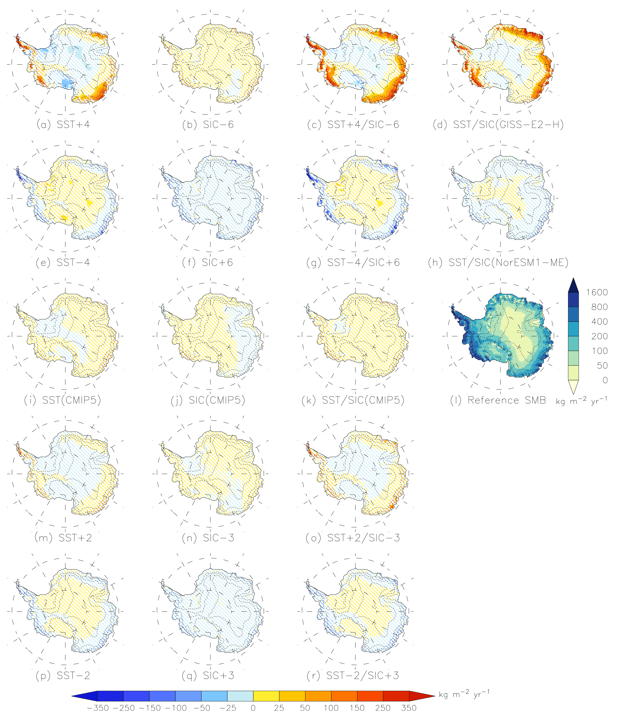
Figure 3Difference in mean annual SMB (kg m−2 yr−1) between the reference simulation and (a) SST +4, (b) SIC −6, (c) SST +4/SIC −6, (d) SST/SIC(GISS-E2-H), (e) SST −4, (f) SIC +6, (g) SST −4/SIC +6, (h) SST/SIC(NorESM1-ME), (i) SST(CMIP5), (j) SIC(CMIP5), (k) SST/SIC(CMIP5), (m) SST +2, (n) SIC −3, (o) SST +2/SIC −3, (p) SST −2, (q) SIC +3, (r) SST −2/SIC+2 experiments. Differences less than the interannual variability are considered as non-significant and are shown by dashed lines. (l) Mean annual SMB (kg m−2 yr−1) simulated by MAR forced by ERA-Interim over 1979–2015.
4.2 Sensitivity to SIC perturbations
A sea ice retreat induces a precipitation increase over the ice sheet, although most of the changes are smaller than the interannual variability (Fig. 3b, n) because it favours the advection of moister air masses towards the AIS, as already suggested by Gallée (1996). In contrast, a sea ice increase produces a negative SMB anomaly driven by the reduction of precipitation over the whole AIS (Fig. 3f, q and Table 2). Similarly, a significant decrease in precipitation is observed over the new ice-covered ocean in SIC +6 (Fig. S4f) because sea ice mainly acts as an isolator preventing evaporation at the ocean surface. Despite the decrease of the mean summer 2 m air temperature by 10 ∘C over new sea ice-covered areas in SIC +3 and SIC +6, surface melting does not exhibit a significant decrease over the ice sheet. The sensitivity of the Antarctic SMB to a decrease in SIC seems to be less pronounced than the sensitivity to an increase in SIC (+3.5 % in SIC −6 vs. −6.6 % in SIC +6). This is likely due to the smaller magnitude of the sea ice retreat in SIC −6 and SIC −3 compared to the magnitude of the sea ice extension in SIC +3 and SIC +6 (Table 1). Finally, the mean SMB from SIC(CMIP5) does not significantly differ from the reference SMB, both spatially (Fig. 3j) and integrated over the whole AIS (Table 2).
4.3 Sensitivity to combined SST/SIC perturbations
Higher SST associated with lower SIC reinforce anomalies found for individual perturbations. Evaporation at the ocean surface is stronger, while warmer air masses have a greater moisture content. Anomalies for integrated precipitation are significantly positive and account for +4.7 % and +12.7 % in the integrated Antarctic SMB for SST +2/SCI −3 and SST +4/SIC −6 respectively (Table 2). Similarly to SST +4 and SST +2, SST +4/SIC −6 and SST +2/SIC −3 show a large conversion of snowfall to rainfall over the ocean and enhanced precipitation rates over near-coastal regions, while the interior of the AIS exhibits lower accumulation rates (Fig. 3c, o). Moreover, snowfall significantly decreases over the Larsen C and George VI ice shelves (both located in the AP) but is largely compensated by rainfall refreezing into the snowpack. Finally, due to higher air temperatures, surface melting and sublimation are also significantly larger. On the contrary, colder SSCs (SST −4/SIC +6 and SST −2/SIC +3) prevent evaporation and result in lower precipitation over the AIS (Table 2), more particularly at the ice sheet margins (Fig. 3g, r). While SSC combined sensitivity experiments over the Greenland ice sheet show similar anomalies to the SST sensitivity experiments (Noël et al., 2014), coupled perturbations act here together to induce larger anomalies over the AIS than the SST sensitivity experiments. Further, the sensitivity of the Antarctic SMB to SSCs is non-linear, illustrating the complexity of the interactions between the (sea ice-covered) ocean surface and the near-surface atmosphere.
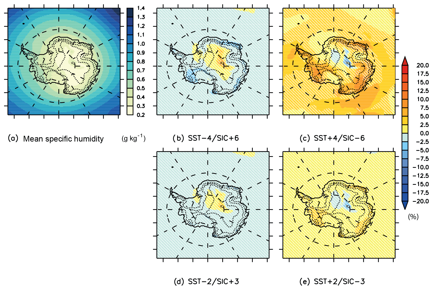
Figure 4(a) Mean specific humidity modelled by MAR over 1979–2015 at 600 hPa (units: g kg−1). Difference in mean specific humidity (%) between the reference simulation and (b) SST −4/SIC +6, (c) SST +4/SIC −6, (d) SST −2/SIC +3, (e) SST +2/SIC −3 experiments. Differences lower than the interannual variability are considered as non-significant and are shown by dashed lines.
As SSC anomalies in SST/SIC(GISS-E2-H) are close in magnitude to anomalies in SST +2/SCI −3 and SST +4/SIC −6, integrated values (Table 2) and spatial anomaly patterns (Fig. 3d) also illustrate the effect of warmer SSCs on the Antarctic SMB by a significant increase in precipitation, sublimation, and melt. However, the spatial pattern of precipitation is slightly different in comparison to SST +4/SIC −6. The precipitation anomaly in SST/SIC(GISS-E2-H) is reduced at the Adélie Land and George V Land margins in comparison to SST +4/SIC −6 due to the positive SIC anomalies in GISS-E2-H over the Ross and D'Urville seas (Fig. 1f). SST/SIC(CMIP5) displays a non-significant positive anomaly for both integrated and spatial SMB (Fig. 3k) as the mean SIC and SST anomalies in CMIP5 models do not significantly differ from the ERA-Interim SSCs (Figs. 1, 3b, e). CMIP5 model anomalies are more or less equally distributed (warm or cold SSC anomalies) around the ERA-Interim SSCs, even if the mean CMIP5 SSCs are slightly warmer than ERA-Interim, explaining the non-significant positive SMB anomaly. Finally, for SST/SIC(NorESM1-ME), SSCs are representative of a colder ocean (lower SST and essentially higher SIC) resulting in a non-significant negative SMB anomaly with a precipitation decrease at the ice edge and over marginal areas of the plateau (Fig. 3h).
Since snowfall is the largest component of the Antarctic SMB, precipitation changes mainly explain the spatial anomaly patterns observed in our experiments. A warmer ocean with a smaller sea ice cover tends to strongly enhance precipitation at the ice sheet margins, while decreased accumulation rates are modelled over the ice shelves and the central part of the ice sheet. These results suggest that precipitation can be formed further inland depending on the properties of air masses. In agreement with Gallée (1996), our hypothesis is that colder and drier air masses in cold ocean experiments are not sufficiently loaded with moisture to enable saturation and then snowfall over the margins. The decrease in moisture is likely to be larger than the decrease in saturation water vapour pressure associated with lower temperatures. This leads to a larger amount of remaining humidity that can be advected further inland (Figs. 4b, d and S10b, d) where saturation occurs because of lower temperatures. On the contrary, the additional humidity in warm ocean experiments results in air masses that reach saturation faster (the increase in humidity overcompensates the increase in saturation water vapour pressure) and thus generate precipitation over the ice sheet slopes. MAR also simulates significantly higher upper-air temperature over the central part of the ice sheet (Figs. S11c, e and S12c, e) that, combined with the lower remaining humidity (Figs. 4c, e and S10c, e), limits snowfall.
Even if our sensitivity experiments rely on larger SSC perturbations than the interannual variability, mean integrated SMB anomalies are not systematically significant in comparison to our reference simulation. Similarly to Van Lipzig et al. (2002), moisture and temperature anomalies remain confined below 700 hPa in the experiments with slightly perturbed SSCs (SST ) (Figs. S10d, e and S12d, e). In contrast, moisture anomalies in the experiments with the largest SSC perturbations (SST ) are not constrained to the boundary layer and reach upper atmospheric layers (600 hPa) (Fig. 4b, c). The blocking effect due to the topographic barrier is likely to be reduced so that these large anomalies influence accumulation rates further inland (Fig. 3c, d, g). Furthermore, katabatic winds are enhanced when the SIC is decreased and the SST increased (Fig. S13c) as already shown in Gallée (1996) and Van Lipzig et al. (2002). Due to their offshore direction, they prevent the influence of warm ocean anomalies by precluding their propagation at the surface of the ice sheet and by advecting cold air from inland regions towards the margins.
In the context of global warming, it is important to note that the Antarctic SMB increases by 2 %–6 % for a SST increase alone and by 5 %–13 % for a SST increase coupled to a SIC drop (Table 2). Similar increases are found in sensitivity experiments based on CMIP5 SSC anomalies compared to ERA-Interim over the current climate (+4 % and +13 % respectively for SST/SIC(CMIP5) and SST/SIC(GISS-E2-H)). Knowing that the regional model RACMO2 projects an increase in SMB by 6 %–16 % in 2100 (Ligtenberg et al., 2013) and the global model LMDZ4 suggests a SMB increase of 17 % for the same horizon (Krinner et al., 2008), our sensitivity tests with warmer (CMIP5-based) oceans reveal SMB anomalies over the current climate in the lower range of the SMB increase projected for the end of the 21st century.
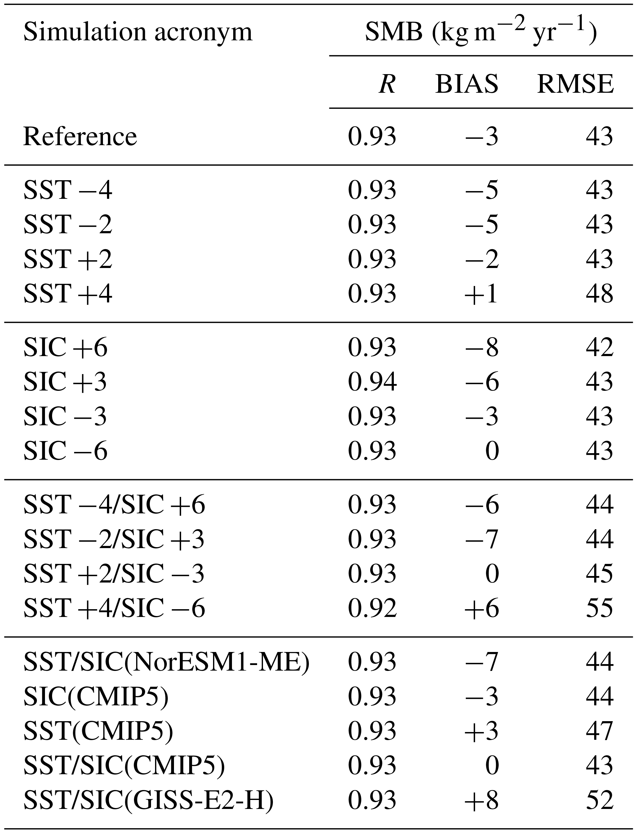
Sensitivity experiments are compared to SMB observations from the GLACIOCLIM-SAMBA dataset with the same methods used for the reference simulation (Sect. 3). Correlation and root mean square error (RMSE) do not vary significantly between the sensitivity experiments and the reference run (Table 3). Only mean biases vary, but the variations are by far smaller than the observed variability. Consequently, sensitivity experiments showing large local or integrated SMB anomalies do not significantly differ from the observed SMB. This is explained by the low number of available observations and highlights the importance of continuing to carry out field campaign measurements, as well as extending their spatial coverage to better evaluate model results.
Table 3Comparison between modelled and observed SMB from the GLACIOCLIM-SAMBA database (Favier et al., 2013) over 1950–2015. Bias and RMSE units are kg m−2 yr−1. The observation mean is 65 kg m−2 yr−1, while the observation standard deviation is 119 kg m−2 yr−1.
Polar-oriented RCMs are suitable numerical tools to study the SMB of the AIS due to their high spatial resolution and adapted physics. Nonetheless, they are forced at their atmospheric and oceanic boundaries by reanalyses or GCM products and are then influenced by their potential biases. These biases can be notably significant for SSCs (Agosta et al., 2015). With the RCM MAR, two sets of sensitivity experiments were carried out to assess the direct response of the Antarctic SMB to oceanic perturbations around Antarctica by perturbing the ERA-Interim SSCs over 1979–2015 while keeping the atmospheric conditions at the MAR lateral and upper boundaries unchanged. The first set consisted of spatially homogeneous SSC perturbations. The second set of experiments involved ERA-Interim SSC perturbations estimated from CMIP5 models anomalies over the current climate. We introduced mean anomalies from the historical run of CMIP5 models and two extreme models of CMIP5, namely NorESM1-ME and GISS-E2-H, respectively representative of warmer and colder SSCs than ERA-Interim.
Results mainly show increased (decreased) precipitation due to warmer (colder) SSCs affecting the SMB of the AIS. As precipitation is mainly caused by low-pressure systems that intrude into the continent and do not penetrate far inland, coastal areas are more sensitive to SSC perturbations with more significant anomalies compared to inland regions. Warmer SSCs significantly enhance precipitation at the ice sheet margins since a greater moisture content of air masses leads to earlier saturation as they rise and adiabatically cool over the topography. On the contrary, colder SSCs reduce precipitation at the ice sheet margins and slightly increase it further inland as air masses have to rise up to higher elevations to reach saturation. Finally, the largest combined SST/SIC perturbations lead to significant (i.e. greater than the interannual variability) SMB anomalies integrated over the whole AIS due to moisture anomalies above the ocean reaching sufficiently high atmospheric levels to influence accumulation rates further inland. However, comparing modelled SMB from sensitivity experiments with observations shows no significant difference, suggesting that large integrated anomalies can remain unperceived when compared to the few field observations.
Our sensitivity tests with warmer (CMIP5-based) SSCs reveal that SMB anomalies over the current climate are in the lower range of the SMB increase projected for the end of the 21st century. Given the influence of SSC perturbations on the Antarctic SMB over the current climate, special attention should be paid to future SMB projections using potentially biased SSCs as forcing. This highlights the necessity of improving the representation of the current-climate SSCs in the context of downscaling the forthcoming CMIP6 model outputs to carry out future Antarctic SMB projections.
The last version of MAR is freely distributed at http://mar.cnrs.fr/ (last access: 22 November 2018). All MARv3.6.4 outputs presented here are available upon request by email (ckittel@uliege.be). The SMB observations (Favier et al., 2013) are available through http://pp.ige-grenoble.fr/pageperso/favier/database.php.
The supplement related to this article is available online at: https://doi.org/10.5194/tc-12-3827-2018-supplement.
CK, ChA, CeA, and XF designed the study. CeA, XF, ChA, and CK developed the MAR model and contributed to the MAR set-up. CK performed the simulations. CK led the writing of the manuscript with ChA. CK, ChA, CeA, PVH, TF, and XF discussed the results, while all co-authors revised and contributed to the editing of the manuscript.
The authors declare that they have no conflict of interest.
We acknowledge the World Climate Research Programme's Working Group on Coupled Modelling, which is responsible for CMIP, and we thank the climate modelling groups for producing their model output and making it available. ERA-Interim data (Dee et al., 2011) are provided by the European Centre for Medium-Range Weather Forecasts, from their website at http://www.ecmwf.int/en/research/climate-reanalysis/era-interim (last access: 22 November 2018).
Computational resources have been provided by the Consortium des Équipements de Calcul Intensif (CÉCI), funded by the Fonds de la Recherche Scientifique de Belgique (F.R.S. – FNRS) under grant no. 2.5020.11 and the Tier-1 supercomputer (Zenobe) of the Fédération Wallonie Bruxelles infrastructure funded by the Walloon Region under grant agreement no. 1117545. This work was supported by the Fonds de la Recherche Scientifique – FNRS under grant no. T.0002.16.
Finally, we would like to thank François Massonnet for fruitful
discussions, and the two anonymous reviewers for their constructive remarks
that helped to improve the paper.
Edited by: Alexander Robinson
Reviewed by: two anonymous referees
Agosta, C., Favier, V., Genthon, C., Gallée, H., Krinner, G., Lenaerts, J. T. M., and van den Broeke, M. R.: A 40-year accumulation dataset for Adelie Land, Antarctica and its application for model validation, Clim. Dynam., 38, 75–86, https://doi.org/10.1007/s00382-011-1103-4, 2012. a
Agosta, C., Fettweis, X., and Datta, R.: Evaluation of the CMIP5 models in the aim of regional modelling of the Antarctic surface mass balance, The Cryosphere, 9, 2311–2321, https://doi.org/10.5194/tc-9-2311-2015, 2015. a, b, c, d, e
Agosta, C., Amory, C., Kittel, C., Orsi, A., Favier, V., Gallée, H., van den Broeke, M. R., Lenaerts, J. T. M., van Wessem, J. M., and Fettweis, X.: Estimation of the Antarctic surface mass balance using MAR (1979–2015) and identification of dominant processes, The Cryosphere Discuss., https://doi.org/10.5194/tc-2018-76, in review, 2018. a, b, c, d, e, f, g, h, i, j, k, l
Amory, C., Trouvilliez, A., Gallée, H., Favier, V., Naaim-Bouvet, F., Genthon, C., Agosta, C., Piard, L., and Bellot, H.: Comparison between observed and simulated aeolian snow mass fluxes in Adélie Land, East Antarctica, The Cryosphere, 9, 1373–1383, https://doi.org/10.5194/tc-9-1373-2015, 2015. a
Amory, C., Gallée, H., Naaim-Bouvet, F., Favier, V., Vignon, E., Picard, G., Trouvilliez, A., Piard, L., Genthon, C., and Bellot, H.: Seasonal Variations in Drag Coefficient over a Sastrugi-Covered Snowfield in Coastal East Antarctica, Bound.-Lay. Meteorol., 164, 107–133, https://doi.org/10.1007/s10546-017-0242-5, 2017. a
Andreas, E. L.: A bulk air-sea flux algorithm for high-wind, spray conditions, version 2.0, in: Preprints, 13th Conference on Interactions of the Sea and Atmosphere, Portland, ME, 9–13 August 2004. a
Bailey, D. A. and Lynch, A. H.: Development of an Antarctic Regional Climate System Model. Part I: Sea Ice and Large-Scale Circulation, J. Climate, 13, 1337–1350, 2000. a
Beaumet, J., Krinner, G., Déqué, M., Haarsma, R., and Li, L.: Assessing bias-corrections of oceanic surface conditions for atmospheric models, Geosci. Model Dev. Discuss., ]doi10.5194/gmd-2017-247, in review, 2017. a
Bentsen, M., Bethke, I., Debernard, J. B., Iversen, T., Kirkevåg, A., Seland, Ø., Drange, H., Roelandt, C., Seierstad, I. A., Hoose, C., and Kristjánsson, J. E.: The Norwegian Earth System Model, NorESM1-M – Part 1: Description and basic evaluation of the physical climate, Geosci. Model Dev., 6, 687–720, https://doi.org/10.5194/gmd-6-687-2013, 2013. a
Bevan, S. L., Luckman, A., Hubbard, B., Kulessa, B., Ashmore, D., Kuipers Munneke, P., O'Leary, M., Booth, A., Sevestre, H., and McGrath, D.: Centuries of intense surface melt on Larsen C Ice Shelf, The Cryosphere, 11, 2743–2753, https://doi.org/10.5194/tc-11-2743-2017, 2017. a
Bracegirdle, T. J. and Marshall, G. J.: The Reliability of Antarctic Tropospheric Pressure and Temperature in the Latest Global Reanalyses, J. Climate, 25, 7138–7146, https://doi.org/10.1175/JCLI-D-11-00685.1, 2012. a
Bromwich, D. H., Chen, B., and Hines, K. M.: Global atmospheric impacts induced by year-round open water adjacent to Antarctica, J. Geophys. Res., 103, 1173–1889, https://doi.org/10.1029/98JD00624, 1998. a, b
Bromwich, D. H., Nicolas, J. P., and Monaghan, A. J.: An Assessment of Precipitation Changes over Antarctica and the Southern Ocean since 1989 in Contemporary Global Reanalyses, J. Climate, 24, 4189–4209, https://doi.org/10.1175/2011JCLI4074.1, 2011. a, b
Brun, E., David, P., Subul, M., and Brunot, G.: A numerical model to simulate snow-cover stratigraphy for operational avalanche forescating, J. Glaciol., 38, 13–22, 1992. a
Cavalieri, D. J. and Parkinson, C. L.: Arctic sea ice variability and trends, 1979–2010, The Cryosphere, 6, 881–889, https://doi.org/10.5194/tc-6-881-2012, 2012. a
Dee, D. P., Uppala, S. M., Simmons, A. J., Berrisford, P., Poli, P., Kobayashi, S., Andrae, U., Balmaseda, M. A., Balsamo, G., Bauer, P., Bechtold, P., Beljaars, A. C. M., van de Berg, L., Bidlot, J., Bormann, N., Delsol, C., Dragani, R., Fuentes, M., Geer, A. J., Haimberger, L., Healy, S. B., Hersbach, H., Hólm, E. V., Isaksen, L., Kållberg, P., Köhler, M., Matricardi, M., Mcnally, A. P., Monge-Sanz, B. M., Morcrette, J. J., Park, B. K., Peubey, C., de Rosnay, P., Tavolato, C., Thépaut, J. N., and Vitart, F.: The ERA-Interim reanalysis: Configuration and performance of the data assimilation system, Q. J. Roy. Meteor. Soc., 137, 553–597, https://doi.org/10.1002/qj.828, 2011. a, b
De Ridder, K. and Gallée, H.: Land surface-induce regional climate change in Southern Israel, J. Appl. Meteorol., 37, 1470–1485, 1998. a
De Ridder, K. and Schayes, G.: The IAGL Land Surface Model, J. Appl. Meteorol., 36, 167–182, https://doi.org/10.1086/451461, 1997. a
Donlon, C. J., Martin, M., Stark, J., Roberts-jones, J., Fiedler, E., and Wimmer, W.: The Operational Sea Surface Temperature and Sea Ice Analysis (OSTIA) system, Remote Sens. Environ., 116, 140–158, https://doi.org/10.1016/j.rse.2010.10.017, 2012. a
Favier, V., Agosta, C., Parouty, S., Durand, G., Delaygue, G., Gallée, H., Drouet, A.-S., Trouvilliez, A., and Krinner, G.: An updated and quality controlled surface mass balance dataset for Antarctica, The Cryosphere, 7, 583–597, https://doi.org/10.5194/tc-7-583-2013, 2013. a, b, c, d
Favier, V., Krinner, G., Amory, C., Gallée, H., Beaumet, J., and Agosta, C.: Antarctica-Regional Climate and Surface Mass Budget, Current Climate Change Reports, 3, 303–315, https://doi.org/10.1007/s40641-017-0072-z, 2017. a
Fettweis, X., Box, J. E., Agosta, C., Amory, C., Kittel, C., Lang, C., van As, D., Machguth, H., and Gallée, H.: Reconstructions of the 1900–2015 Greenland ice sheet surface mass balance using the regional climate MAR model, The Cryosphere, 11, 1015–1033, https://doi.org/10.5194/tc-11-1015-2017, 2017. a
Fiorino, M.: A multi-decadal daily sea surface temperature and sea ice concentration data set for the ERA-40 reanalysis, ECMWF, Reading, UK, ERA-40 Project Report Series No. 12, 1–22, 2004. a
Franco, B., Fettweis, X., Lang, C., and Erpicum, M.: Impact of spatial resolution on the modelling of the Greenland ice sheet surface mass balance between 1990–2010, using the regional climate model MAR, The Cryosphere, 6, 695–711, https://doi.org/10.5194/tc-6-695-2012, 2012. a
Fretwell, P., Pritchard, H. D., Vaughan, D. G., Bamber, J. L., Barrand, N. E., Bell, R., Bianchi, C., Bingham, R. G., Blankenship, D. D., Casassa, G., Catania, G., Callens, D., Conway, H., Cook, A. J., Corr, H. F. J., Damaske, D., Damm, V., Ferraccioli, F., Forsberg, R., Fujita, S., Gim, Y., Gogineni, P., Griggs, J. A., Hindmarsh, R. C. A., Holmlund, P., Holt, J. W., Jacobel, R. W., Jenkins, A., Jokat, W., Jordan, T., King, E. C., Kohler, J., Krabill, W., Riger-Kusk, M., Langley, K. A., Leitchenkov, G., Leuschen, C., Luyendyk, B. P., Matsuoka, K., Mouginot, J., Nitsche, F. O., Nogi, Y., Nost, O. A., Popov, S. V., Rignot, E., Rippin, D. M., Rivera, A., Roberts, J., Ross, N., Siegert, M. J., Smith, A. M., Steinhage, D., Studinger, M., Sun, B., Tinto, B. K., Welch, B. C., Wilson, D., Young, D. A., Xiangbin, C., and Zirizzotti, A.: Bedmap2: improved ice bed, surface and thickness datasets for Antarctica, The Cryosphere, 7, 375–393, https://doi.org/10.5194/tc-7-375-2013, 2013. a
Frezzotti, M., Scarchilli, C., Becagli, S., Proposito, M., and Urbini, S.: A synthesis of the Antarctic surface mass balance during the last 800 yr, The Cryosphere, 7, 303–319, https://doi.org/10.5194/tc-7-303-2013, 2013. a
Gallée, H.: Simulation of the Mesocyclonic Activity in the Ross Sea, Antarctica, Mon. Weather Rev., 123, 2051–2069, https://doi.org/10.1175/1520-0493(1995)123<2051:SOTMAI>2.0.CO;2, 1995. a, b, c
Gallée, H.: Mesoscale Atmospheric Circulations over the Southwestern Ross Sea Sector, Antarctica, J. Appl. Meteorol., 35, 1129–1141, 1996. a, b, c, d, e, f
Gallée, H. and Duynkerke, P. G.: Air-snow interactions and the surface energy and mass balance over the melting zone of west Greenland during the Greenland Ice Margin Experiment, J. Geophys. Res., 102, 13813–13824, https://doi.org/10.1029/96JD03358, 1997. a
Gallée, H. and Schayes, G.: Development of a Three-Dimensional Meso-γ Primitive Equation Model: Katabatic Winds Simulation in the Area of Terra Nova Bay, Antarctica, Mon. Weather Rev., 122, 671–685, https://doi.org/10.1175/1520-0493(1994)122<0671:DOATDM>2.0.CO;2, 1994. a
Gallée, H., Guyomarc'h, G., and Brun, E.: Impact of snow drift on the antarctic ice sheet surface mass balance: Possible sensitivity to snow-surface properties, Bound.-Lay. Meteorol., 99, 1–19, https://doi.org/10.1023/A:1018776422809, 2001. a, b
Gallée, H., Preunkert, S., Argentini, S., Frey, M. M., Genthon, C., Jourdain, B., Pietroni, I., Casasanta, G., Barral, H., Vignon, E., Amory, C., and Legrand, M.: Characterization of the boundary layer at Dome C (East Antarctica) during the OPALE summer campaign, Atmos. Chem. Phys., 15, 6225–6236, https://doi.org/10.5194/acp-15-6225-2015, 2015. a
Krinner, G., Guicherd, B., Ox, K., Genthon, C., and Magand, O.: Influence of oceanic boundary conditions in simulations of antarctic climate and surface mass balance change during the coming century, J. Climate, 21, 938–962, https://doi.org/10.1175/2007JCLI1690.1, 2008. a, b
Krinner, G., Largeron, C., Ménégoz, M., Agosta, C., and Brutel-Vuilmet, C.: Oceanic forcing of Antarctic climate change: A study using a stretched-grid atmospheric general circulation model, J. Climate, 27, 5786–5800, https://doi.org/10.1175/JCLI-D-13-00367.1, 2014. a, b
Lang, C., Fettweis, X., and Erpicum, M.: Stable climate and surface mass balance in Svalbard over 1979–2013 despite the Arctic warming, The Cryosphere, 9, 83–101, https://doi.org/10.5194/tc-9-83-2015, 2015. a
Lefebre, F., Gallée, H., VanYpersele, J., and Greuell, W.: Modeling of snow and ice melt at ETH Camp (West Greenland): A study of surface albedo, J. Geophys. Res., 108, 4231, https://doi.org/10.1029/2001JD001160, 2003. a
Lenaerts, J. T. M., Van Den Broeke, M. R., Van De Berg, W. J., Van Meijgaard, E., and Kuipers Munneke, P.: A new, high-resolution surface mass balance map of Antarctica (1979–2010) based on regional atmospheric climate modeling, Geophys. Res. Lett., 39, L04501, https://doi.org/10.1029/2011GL050713, 2012. a
Li, L. and Pomeroy, J. W.: Estimates of threshold wind speeds for snow transport using meteorological data, J. Appl. Meteorol., 36, 205–213, https://doi.org/10.1175/1520-0450(1997)036<0205:EOTWSF>2.0.CO;2, 1997. a
Ligtenberg, S. R. M., Rae, J. G. L., and Meijgaard, E. V.: Future surface mass balance of the Antarctic ice sheet and its influence on sea level change, simulated by a regional atmospheric climate model, Clim. Dynam., 41, 867–884, https://doi.org/10.1007/s00382-013-1749-1, 2013. a
Mahlstein, I., Gent, P. R., and Solomon, S.: Historical Antarctic mean sea ice area, sea ice trends, and winds in CMIP5 simulations, J. Geophys. Res.-Atmos., 118, 5105–5110, https://doi.org/10.1002/jgrd.50443, 2013. a
Massonnet, F., Mathiot, P., Fichefet, T., Goosse, H., König Beatty, C., Vancoppenolle, M., and Lavergne, T.: A model reconstruction of the Antarctic sea ice thickness and volume changes over 1980-2008 using data assimilation, Ocean Model., 64, 67–75, https://doi.org/10.1016/j.ocemod.2013.01.003, 2013. a
Messager, C., Gallée, H., and Brasseur, O.: Precipitation sensitivity to regional SST in a regional climate simulation during the West African monsoon for two dry years, Clim. Dynam., 22, 249–266, https://doi.org/10.1007/s00382-003-0381-x, 2004. a
Noël, B., Fettweis, X., van de Berg, W. J., van den Broeke, M. R., and Erpicum, M.: Sensitivity of Greenland Ice Sheet surface mass balance to perturbations in sea surface temperature and sea ice cover: a study with the regional climate model MAR, The Cryosphere, 8, 1871–1883, https://doi.org/10.5194/tc-8-1871-2014, 2014. a, b, c, d, e
Noone, D. and Simmonds, I.: Sea ice control of water isotope transport to Antarctica and implications for ice core interpretation, J. Geophys. Res., 109, D07105, https://doi.org/10.1029/2003JD004228, 2004. a
Parkinson, C. L. and Cavalieri, D. J.: Antarctic sea ice variability and trends, 1979–2010, The Cryosphere, 6, 871–880, https://doi.org/10.5194/tc-6-871-2012, 2012. a
Roach, L. A., Dean, S. M., and Renwick, J. A.: Consistent biases in Antarctic sea ice concentration simulated by climate models, The Cryosphere, 12, 365–383, https://doi.org/10.5194/tc-12-365-2018, 2018. a, b
Schmidt, G. A., Kelley, M., Nazarenko, L., Ruedy, R., Russell, G. L., Aleinov, I., Bauer, M., Bauer, S. E., Bhat, M. K., Bleck, R., Canuto, V., Chen, Y.-H., Cheng, Y., Clune, T. L., Del Genio, A., de Fainchtein, R., Faluvegi, G., Hansen, J. E., Healy, R. J., Kiang, N. Y., Koch, D., Lacis, A. A., LeGrande, A. N., Lerner, J., Lo, K. K., Matthews, E. E., Menon, S., Miller, R. L., Oinas, V., Oloso, A. O., Perlwitz, J. P.. Puma, M. J., Putman, W. M., Rind, D., Romanou, A., Sato, M., Shindell, D. T., Sun, S., Syed, R. A., Tausnev, N., Tsigaridis, K., Unger, N., Voulgarakis, A., Yao, M.-S., and Zhang, J.: Configuration and assessment of the GISS ModelE2 contributions to the CMIP5 archive, J. Adv. Model. Earth Sy., 6, 141–184, 2014. a
Shu, Q., Song, Z., and Qiao, F.: Assessment of sea ice simulations in the CMIP5 models, The Cryosphere, 9, 399–409, https://doi.org/10.5194/tc-9-399-2015, 2015. a
Simmonds, I. and Budd, W. F.: Sensitivity of the southern hemisphere circulation to leads in the Antarctic pack ice, Q. J. Roy. Meteor. Soc., 117, 1003–1024, https://doi.org/10.1002/qj.49711750107, 1991. a
Simmonds, I. and Jacka, T.: Relationships between the interannual variability of Antarctic sea ice and the southern oscillation, J. Climate, 8, 637–647, 1995. a
Simmonds, I. and Wu, X.: Cyclone behaviour response to changes in winter southern hemisphere sea-ice concentration, Q. J. Roy. Meteor. Soc., 119, 1121–1148, https://doi.org/10.1002/qj.49711951313, 1993. a
Sodemann, H. and Stohl, A.: Asymmetries in the moisture origin of Antarctic precipitation, Geophys. Res. Lett., 36, L22803, https://doi.org/10.1029/2009GL040242, 2009. a
Stark, J. D., Donlon, C. J., Martin, M. J., and McCulloch, M. E.: OSTIA: An operational, high resolution, real time, global sea surface temperature analysis system, in: Oceans 2007 – Europe, Aberdeen, UK, 18–21 June 2007, IEEE, 1–4, https://doi.org/10.1109/OCEANSE.2007.4302251, 2007. a
Taylor, K. E., Stouffer, R. J., and Meehl, G. A.: An overview of CMIP5 and theexperiment design, B. Am. Meteorol. Soc., 93, 485–498, 2012. a
Turner, J., Bracegirdle, T. J., Phillips, T., Marshall, G. J., and Scott Hosking, J.: An initial assessment of antarctic sea ice extent in the CMIP5 models, J. Climate, 26, 1473–1484, https://doi.org/10.1175/JCLI-D-12-00068.1, 2013. a
Turner, J., Scott Hosking, J., Marshall, G. J., Phillips, T., and Bracegirdle, T. J.: Antarctic sea ice increase consistent with intrinsic variability of the Amundsen sea low, Clim. Dynam., 46, 2391–2402, https://doi.org/10.1007/s00382-015-2708-9, 2016. a
Uppala, S. M., Kållberg, P. W., Simmons, A. J., Andrae, U., Bechtold, V. D. C., Fiorino, M., Gibson, J. K., Haseler, J., Hernandez, A., Kelly, G. A., Li, X., Onogi, K., Saarinen, S., Sokka, N., Allan, R. P., Andersson, E., Arpe, K., Balmaseda, M. A., Beljaars, A. C. M., Berg, L. V. D., Bidlot, J., Bormann, N., Caires, S., Chevallier, F., Dethof, A., Dragosavac, M., Fisher, M., Fuentes, M., Hagemann, S., Hólm, E., Hoskins, B. J., Isaksen, L., Janssen, P. A. E. M., Jenne, R., Mcnally, A. P., Mahfouf, J.-F., Morcrette, J.-J., Rayner, N. A., Saunders, R. W., Simon, P., Sterl, A., Trenberth, K. E., Untch, A., Vasiljevic, D., Viterbo, P., and Woollen, J.: The ERA-40 re-analysis, Q. J. Roy. Meteor. Soc., 131, 2961–3012, https://doi.org/10.1256/qj.04.176, 2005. a
van de Berg, W. J. and Medley, B.: Brief Communication: Upper-air relaxation in RACMO2 significantly improves modelled interannual surface mass balance variability in Antarctica, The Cryosphere, 10, 459–463, https://doi.org/10.5194/tc-10-459-2016, 2016. a
Van Lipzig, N. P. M., Van Meijgaard, E., and Oerlemans, J.: Temperature sensitivity of the Antarctic surface mass balance in a regional atmospheric climate model, J. Climate, 15, 2758–2774, https://doi.org/10.1175/1520-0442(2002)015<2758:TSOTAS>2.0.CO;2, 2002. a, b, c, d
van Wessem, J. M., van de Berg, W. J., Noël, B. P. Y., van Meijgaard, E., Amory, C., Birnbaum, G., Jakobs, C. L., Krüger, K., Lenaerts, J. T. M., Lhermitte, S., Ligtenberg, S. R. M., Medley, B., Reijmer, C. H., van Tricht, K., Trusel, L. D., van Ulft, L. H., Wouters, B., Wuite, J., and van den Broeke, M. R.: Modelling the climate and surface mass balance of polar ice sheets using RACMO2 – Part 2: Antarctica (1979–2016), The Cryosphere, 12, 1479–1498, https://doi.org/10.5194/tc-12-1479-2018, 2018. a
Wang, Y.: An Explicit Simulation of Tropical Cyclones with a Triply Nested Movable Mesh Primitive Equation Model: TCM3. Part I: Model Description and Control Experiment, Mon. Weather Rev., 1129, 1370–1394, https://doi.org/10.1175/1520-0493(2002)130<3022:AESOTC>2.0.CO;2, 2001. a
Weatherly, J.: Sensitivity of Antarctic Precipitation to Sea Ice Concentrations in a General Circulation Model, J. Climate, 17, 3214–3223, 2004. a, b
Wu, X. G., Simmonds, I., and Budd, W. F.: Southern hemisphere climate system recovery from 'instantaneous' sea-ice removal, Q. J. Roy. Meteor. Soc., 122, 1501–1520, 1996. a