the Creative Commons Attribution 4.0 License.
the Creative Commons Attribution 4.0 License.
 | 08 Nov 2018
Repeat mapping of snow depth across an alpine catchment with RPAS photogrammetry
Todd A. N. Redpath
Pascal Sirguey
Nicolas J. Cullen
Being dynamic in time and space, seasonal snow represents a difficult target for ongoing in situ measurement and characterisation. Improved understanding and modelling of the seasonal snowpack requires mapping snow depth at fine spatial resolution. The potential of remotely piloted aircraft system (RPAS) photogrammetry to resolve spatial variability of snow depth is evaluated within an alpine catchment of the Pisa Range, New Zealand. Digital surface models (DSMs) at 0.15 m spatial resolution in autumn (snow-free reference) winter (2 August 2016) and spring (10 September 2016) allowed mapping of snow depth via DSM differencing. The consistency and accuracy of the RPAS-derived surface was assessed by the propagation of check point residuals from the aero-triangulation of constituent DSMs and via comparison of snow-free regions of the spring and autumn DSMs. The accuracy of RPAS-derived snow depth was validated with in situ snow probe measurements. Results for snow-free areas between DSMs acquired in autumn and spring demonstrate repeatability yet also reveal that elevation errors follow a distribution that substantially departs from a normal distribution, symptomatic of the influence of DSM co-registration and terrain characteristics on vertical uncertainty. Error propagation saw snow depth mapped with an accuracy of ±0.08 m (90 % c.l.). This is lower than the characterization of uncertainties on snow-free areas (±0.14 m). Comparisons between RPAS and in situ snow depth measurements confirm this level of performance of RPAS photogrammetry while also highlighting the influence of vegetation on snow depth uncertainty and bias. Semi-variogram analysis revealed that the RPAS outperformed systematic in situ measurements in resolving fine-scale spatial variability. Despite limitations accompanying RPAS photogrammetry, which are relevant to similar applications of surface and volume change analysis, this study demonstrates a repeatable means of accurately mapping snow depth for an entire, yet relatively small, hydrological catchment (∼0.4 km2) at very high resolution. Resolving snowpack features associated with redistribution and preferential accumulation and ablation, snow depth maps provide geostatistically robust insights into seasonal snow processes, with unprecedented detail. Such data will enhance understanding of physical processes controlling spatial distributions of seasonal snow and their relative importance on varying spatial and temporal scales.
- Article
(5516 KB) - Full-text XML
- BibTeX
- EndNote


Seasonal snow provides a globally important water resource (Mankin et al., 2015; Sturm et al., 2017), which is highly variable in space and time (Clark et al., 2011). Difficulties associated with collecting field observations limit the characterisation and understanding of spatial variability in snow depth and, in turn, our ability to improve spatially distributed modelling of seasonal snow. While insight can be gained via modelling on moderate to large scales (Winstral et al., 2013), resolving the fine-scale variability and its controlling processes remains limited by the ability to capture such variability in the field (Clark et al., 2011). Since water storage within a snowpack is a function of snow depth and density, and the former exhibits higher spatial variability than the latter, advances in measuring snow depth at high spatial resolution offer promise for improved estimates of snow water equivalent (SWE) (Harder et al., 2016).
Historically, studies of seasonal snow processes have relied on in situ observations. With biweekly temporal resolution, Anderson et al. (2014) gained substantial insights into physical controls on seasonal snow processes, albeit with a dependence on statistical scaling to relate transect-scale observations to basin-scale processes. Alternatively, the nature of automated snow measurement instrumentation often precludes continuous in situ measurement across networks sufficiently dense to characterise fine-scale spatial variability. Kinar and Pomeroy (2015) provide a comprehensive review of instrumentation and techniques for measuring snow depth and characterising snowpacks. In summary, while instrumentation and methodologies exist for obtaining accurate and temporally continuous, measurements of snow depth and related snowpack properties at point locations, adequately resolving the high spatial variability of snow depth remains a challenge. This is exacerbated by local field conditions, such as exposure to wind or the complexity of the topography and vegetation further increasing the spatial variability in snow depth (Clark et al., 2011; Kerr et al., 2013; Winstral and Marks, 2014).
Remote sensing has provided substantial advances in quantification of seasonal snow variability, with imaging sensors supporting spatial and temporal resolutions that allow a range of scales to be explored. Space-borne satellite imagers provide a synoptic view and accompanying step-change capability in capturing properties of snow-covered areas, although trade-offs exist between competing spatial, spectral and temporal resolutions (Dozier, 1989; Nolin and Dozier, 1993; Hall et al., 2002, 2015; Sirguey et al., 2009; Malenovský et al., 2012; Rittger et al., 2013; Roy et al., 2014; Bessho et al., 2016). Passive and active microwave sensors offer the capacity to retrieve estimates of snow water equivalent directly from space-borne platforms but also suffer substantial limitations, including coarse spatial resolution in the case of passive microwave sensors and complexities in successfully processing snow signals and accounting for complex terrain in the case of both passive and active sensors (Lemmetyinen et al., 2018). Despite the progress in remotely mapping snow, reliable determination of snow depth, particularly in complex terrain, remains challenging. Modern, very high-resolution stereo-capable imagers show promise for retrieving snow depth over large areas from space, although the influence of topography on uncertainties and complications introduced by shadows in alpine terrain demand attention (Marti et al., 2016).
Advances in light detection and ranging (lidar) technologies have become increasingly relevant for measurement of snow depth, firstly from air (Deems et al., 2013; Painter et al., 2016) and more recently from space-borne platforms (Treichler and Kääb, 2017). Of the three modes of lidar data capture, terrestrial laser scanning (TLS) (e.g. Revuelto et al., 2016) offers the best performance in terms of precision and accuracy. TLS can resolve snow depth on a fine scale across relatively large areas but remains limited by view-obstruction and logistical challenges of placing equipment in situ in complex terrain. Airborne lidar provides a balance of spatial resolution and accurate surface elevation measurement and, combined with density estimates, can provide SWE estimates on the catchment scale across substantial areas of hundreds of square kilometres (Painter et al., 2016). High financial costs and logistical challenges, however, preclude regular airborne lidar data capture in many regions globally. Treichler and Kääb (2017) assessed ICESat lidar data, which is designed primarily for measuring surface elevation over polar regions to characterise seasonal snow depth in subpolar southern Norway. Despite reasonable estimates of snow depth, measurements were accompanied by relatively large errors for most temperate locations. ICESat measurements are also limited by their punctual nature and footprint, yielding a relatively sparse and coarse spatial distribution, in turn complicating inferences about spatial variability.

Recent technological advances, including the miniaturisation of imaging and positioning sensors, as well as improvements in battery power and autonomous navigation have significantly lowered the barriers associated with a remotely piloted aircraft system (RPAS, also known as unmanned aerial systems, UAS, and unmanned aerial vehicles) operation (Watts et al., 2012). This, combined with ever-increasing computing power and significant improvements in machine-vision for dense photogrammetric reconstruction (Hirschmuller, 2008; Lindeberg, 2015), provides new opportunities to map small areas photogrammetrically at very high resolution in a temporally flexible, on-demand, fashion. Examples of RPAS use related to mapping snow depth are promising but tend to apply to sub-catchment scales and to not fully characterise the uncertainty associated with photogrammetric modelling (Vander Jagt et al., 2015; Bühler et al., 2016; De Michele et al., 2016; Harder et al., 2016, Cimoli et al., 2017; Avanzi et al., 2018). Furthermore, most RPAS studies of snow depth to date have mapped terrain of relatively low complexity (e.g. Avanzi et al., 2018; Fernandes et al., 2018). Additionally, with a few exceptions (e.g. Harder et al., 2016; Bühler et al., 2017; Marti et al., 2016), previous studies have often relied on multirotor platforms despite their relatively short endurance and reduced spatial coverage relative to fixed-wing alternatives. Merit remains in characterising fine-scale variability in snow depth distribution across an entire catchment, a scale that fixed-wing RPAS can more easily capture. However, increased terrain complexity and the magnitude of the image block can, in turn, challenge photogrammetric modelling. Determination of snow depth via RPAS photogrammetry relies first on the reconstruction of three-dimensional scenes from a set of overlapping images and then on the principal of differencing between temporally subsequent surfaces, provided by point clouds or digital surface models (DSMs) (Vander Jagt et al., 2015; Harder et al., 2016). A snow-free surface provides a reference data set for absolute snow depth, while changes in snow distribution through winter can be assessed by comparing surfaces obtained while snow cover is present in the catchment. Because changes in snow depth through time, either through processes of accumulation, ablation or redistribution, may be subtle, the repeatability and vertical accuracy achieved by photogrammetric modelling is paramount. The aim of this paper is to test a methodology for retrieving snow depth across an entire catchment via RPAS photogrammetry from a fixed-wing platform. We seek to evaluate the performance, limitations and usefulness of this approach and assess how well snow depth can be resolved on the catchment scale. Associated challenges include minimising spatial uncertainties sufficiently to reliably detect changes in snow depth over time, with a decimetre level of vertical accuracy targeted, while also reducing the need and complication of extensive in situ collection of ground control points (GCPs). This approach was assessed during a campaign of winter RPAS-based photogrammetric surveys of an alpine catchment in the Pisa Range, New Zealand, was undertaken.
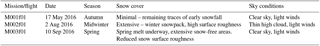
Table 1Timing details for RPAS flights during 2016. All flights were completed between noon and early afternoon.
The paper describes the field site, field and photogrammetric methods, as well as the quality and accuracy assessment. Results are considered in terms of the validation and repeatability of the method, as well as considering the spatial distribution of snow within the catchment. The discussion addresses the performance of RPAS photogrammetry in this context, sources and nature of the associated uncertainty as well as pitfalls and limitations that were encountered, before demonstrating the insight that RPAS-derived data can provide for the study of seasonal snow. While primarily exploring and assessing the potential of RPAS photogrammetry for measuring seasonal snowpack, this study has broader implications for the wider field of modern close-range photogrammetry, as typically implemented from low-cost (relative to manned systems) unmanned systems. While considered here in terms of seasonal snow, the characterisation of RPAS photogrammetry performance presented also applies to other applications involving three-dimensional surface and/or volume change analysis.
The study catchment (Fig. 1), a tributary of the Leopold Burn located in the Pisa Range of the Southern Alps/Kā Tiritiri-o-te-Moana of New Zealand (44.882∘ S, 169.081∘ E), is 0.41 km2 in size and has been the subject of prior snow-hydrology investigations (Sims and Orwin, 2011). Elevation of the catchment ranges between 1440 and 1580 m a.s.l. with a near-uniform area-elevation distribution (Fig. 1). The average slope is moderate, with 80 % of the catchment having a surface slope of 24∘ or less. The catchment runs north to south and is drained by a small stream. While east of the Main Divide of the Southern Alps, the Pisa Range is representative of several large fault-block mountain ranges that dominate the eastern portion of the Clutha Catchment within the Otago region. These ranges are bounded by moderately steep slopes, rising to broad continuous ridge and plateau systems, in turn dissected by relatively shallow gullies, basins and gorges. These ranges feature relatively large areas above the winter snowline, with complex micro-terrain features, which are of interest in the context of redistribution, preferential accumulation and ablation of seasonal snow. In combination with typically windy conditions, the topography is expected to produce complex, highly variable spatial distributions of seasonal snow, convolved with and potentially overtaking the role of elevation in influencing variability in snow depth. The catchment mapped in this study is larger than areas mapped for similar studies published to date (Vander Jagt et al., 2015; Bühler et al., 2016; De Michele et al., 2016; Harder et al., 2016) and has a relatively complex topography, with several gullies dissecting the main slopes, separated by broad, steep-sided ridges. Visual assessment of Landsat, Sentinel-2, and MODIS imagery revealed that, while the catchment could be considered to be in the marginal snow zone, snow cover persists from June to late September in most years, thus providing opportunities for repeated mapping and the capture of the snowpack in various states.
3.1 Field approach
3.1.1 RPAS platform and payload
We used the Trimble UX5 Unmanned Aircraft System, a fixed-wing RPAS manufactured by Trimble Navigation for photogrammetric applications. A single two-blade propeller, driven by a 700 W electric motor, propels the platform. Power is supplied from a 14.8 V, 6000 mAh lithium-polymer battery allowing a flight endurance of 50 min. Autonomous navigation is supported by a single-channel GPS receiver, which also provides approximate coordinates for each photo centre, while an accelerometer logs orientation data.
Imagery is captured by a large-sensor (APS-C) Sony NEX 5R mirrorless reflex digital camera providing a maximum imaging resolution of 4912 pixels by 3264 pixels or about 0.04 m GSD at 400 ft (122 m) a.g.l. The camera is fitted with a Voigtlander Super Wide-Heliar 15 mm f/4.5 Aspherical II lens, with focus fixed to infinity. Appropriate exposure to ensure suitable contrast on the range of imaged targets was achieved with maximum aperture, high shutter speeds between 1∕1000 and 1∕4000 s to minimize forward-motion blurring and automatic ISO sensitivity. Camera settings were checked prior to each flight to accommodate varying light conditions and the relative share of ground cover (vegetation vs. snow).
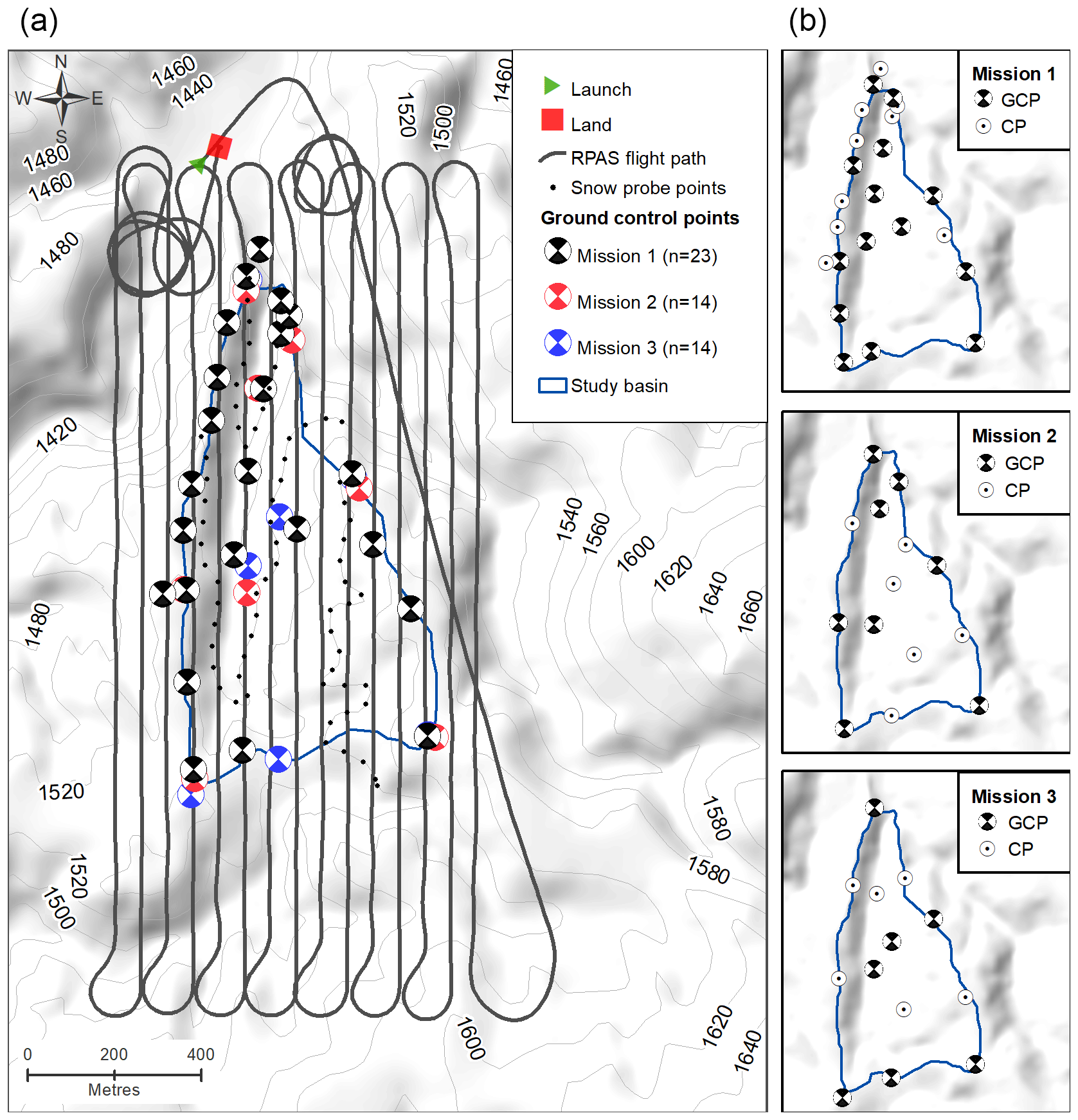
Figure 2Typical flight path for the mapping of the study catchment using the Trimble UX5, GCP network established for each flight mission, and reference snow depth locations. Flight log is from the spring flight mission. The configuration of the ground control point (GCP) and check point (CP) assignment for the triangulation of each flight is shown in the panels on the right-hand side.
3.1.2 RPAS flights
Three RPAS missions were undertaken with identical planning and differing states of snow cover in the catchment (Table 1). Flight planning was carried out using the Trimble Aerial Imaging software. All flights imaged 15 strips, aligned along the major axis of the study catchment (Fig. 2). The study area was imaged with 90/80 % forward/sideward overlap with respect to the lowest elevation to ensure that sufficient overlap was maintained when mapping rising ground. Exposure locations are determined automatically by the software to achieve the desired overlap, with the camera being triggered accordingly during flight using on-board Global Navigation Satellite System (GNSS) navigation. The duration of each flight was ∼35 min, with about 900 images being captured per flight. The average flying altitude of the flights was 1650 m a.s.l., with a standard deviation of less than 1.5 m during the mapping phase of the flight. For both the winter and spring flights, the snow surface had considerable texture, with a greater surface roughness overall for winter missions. Wind-affected recent fresh snow was present for the winter flight. It is recognised that homogeneous snow surfaces may represent particularly challenging targets for photogrammetry (Bühler et al., 2017). Nevertheless, the imaging quality and dynamic range of the camera used in this study provided sufficient contrast for all flights, across snow as well as when imaging mixed snow-bare ground conditions. Subsequently, full photogrammetric restitution could be completed without the need for image post-processing (e.g. Cimoli et al., 2017).
3.1.3 Ground control survey
Achieving a robust constraint of exterior orientation parameters during aero-triangulation (AT) depends on the availability of a set of high-quality ground control points (GCPs). This is particularly true if the imaging platform lacks a precise-point-positioning capability (e.g. it carries only single-frequency GPS and is not capable of determining differentially corrected positions). Such code-only GPS navigation is accompanied by uncertainties 2 orders of magnitude greater than the expected accuracy of the models. Ground control networks were established for each RPAS flight mission using real-time kinematic (RTK) GNSS surveying with a Trimble R7 base station and R6 rover units. GCP locations were measured with accuracy of the order of ∼0.02–0.03 m. GCPs were signalled with 0.6×0.6 m mats painted with a high-contrast circular quadrant pattern for the autumn and winter flights. For the spring flight, chalk powder was used with a stencil to mark the target directly on the snow surface, using the same pattern as for previous flights. The use of chalk powder eliminated the need to retrieve GCP targets following RPAS flights. All survey work, as well as production of deliverables from photogrammetry, was carried out in terms of the New Zealand Transverse Mercator (NZTM) reference system. All RTK survey work utilised a base station established on a common benchmark, established for this project, the position of which was differentially corrected with respect to nearby continually operating reference stations. GNSS data were processed using Trimble Business Center (TBC) v3.40 software.
It is well established that photogrammetric control is best achieved within the bounds of the GCP network (Linder, 2016), while the uncertainty associated with the geolocation of resected points increases beyond the control network. To constrain the area within the study catchment for photogrammetric processing, the GCP network was distributed around the catchment perimeter, as well as through the central area of the catchment. Additionally, the placement of GCPs on the valley floor and at mid-elevation within the catchment ensured that the network also sampled the elevation range of the catchment. An extensive GCP network was established for the first flight with no snow on the ground, which permitted the robustness of AT to be tested under different GCP scenarios, as discussed further in Sect. 3.2.1. This allowed the network to be refined and reduced in size for subsequent missions, a matter of practical importance when working in alpine areas during the winter. Control point networks for each mission are illustrated in Fig. 2. A new GCP network was established for each survey campaign due to the inability to establish permanent markers (e.g. on poles) due to the conservation status of the study area. Although the layout of the network was similar for each mission, there were no common GCPs shared between different flights, with the only common setting being the set-up of the base station for each RTK survey.
3.1.4 Reference snow depth measurements
To assess the quality of snow depth data derived from RPAS photogrammetry, independent measurements were collected by manual snow probing on 10 September 2016, the same day as the spring RPAS mission. This approach has been established as standard practice in similar studies (e.g. Nolan et al., 2015; De Michele et al., 2016). Aluminium avalanche probes with 0.01 m graduations, providing a nominal precision of 0.01 m, were used. The sampling strategy involved the measurement of snow depth every 50 m along three elevation contours within the study catchment, namely 1460, 1500 and 1540 m (Fig. 2). This strategy ensured that snow depth was measured across a representative sample of slope aspect and elevation, while optimizing navigation across the catchment. Snow depths were measured at each location by probing 5 times within arm's reach, and the location of the central measurement was surveyed with RTK GNSS, under the same protocol and achieving the same level of accuracy as the GCP survey. This provided 430 measurements of snow depth, with the mean snow depth at each of the 86 locations providing a sample for comparisons with RPAS-derived snow depth.
3.2 Data processing
3.2.1 Photogrammetric processing
The goal of aero-triangulation (AT) in photogrammetry is to transform a set of images into a scene in which geometrically accurate measurements can be made in three-dimensional, often geographic, space. This georeferencing process requires a transformation from the inherent coordinate system of the device capturing imagery (a camera) to an appropriate geographic coordinate system (Vander Jagt et al., 2015; Linder, 2016). While traditional photogrammetry has long relied on metric (calibrated) cameras, the use of off-the-shelf non-metric cameras requires the simultaneous solving of both interior orientation (the camera model) and exterior orientation. This process, known as self-calibration, applies a bundle-block adjustment to solve the camera model describing the precise focal length (f), the offset between the principal point of autocollimation and the centre of the imaging sensor plane (x0, y0), and the departure between the image point coordinate (x, y) and the idealized linear projection due to lens distortion. Camera calibration parameterises radial and decentering distortion with models such as that of Brown (1971):
in which K terms are the radial distortion coefficients, T terms are the tangential distortion coefficients, and
Image coordinates corrected for lens distortion are then used in the set of collinearity equations relating object point coordinates (XA, YA, ZA) to the corresponding image point coordinates (, ) to solve for the exterior orientation (Vander Jagt et al., 2015; Linder, 2016):
(X0, Y0, Z0) are the coordinates of the perspective centre of the image frame in the ground coordinate system. The rij terms represent the 3×3 rotation matrix relating the sensor coordinate system orientation to the ground coordinate system. Since the UX5 camera is fixed with respect to the platform, the latter combines the roll, pitch and yaw (ω, φ, κ) of the platform at the time of exposure. The nature of bundle-block adjustment with camera self-calibration dictates that the quality of the final photogrammetric model is highly sensitive to errors in both sensor position and orientation as well as inaccurate refinements of the interior orientation parameters (Ebner and Fritz, 1980).
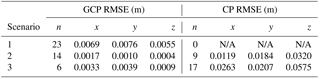
Table 2Summary results of alternative ground control point (GCP) and check point (CP) scenarios tested for aero-triangulation within UAS Master.
3.2.2 Software and workflow
Initially, AT was carried out using the photogrammetry module of Trimble Business Center, v3.40 (TBC), which relies on a simplified implementation of the adjustment process from Inpho UAS Master. Deliverables produced using TBC, however, suffered from severe elevation artefacts which limited their usefulness for further analysis. This is discussed further in Sect. 5.3.
Following the identification of shortfalls in TBC, AT was carried out using Trimble Inpho UAS Master® v8.0 (UAS Master). UAS Master is a feature-rich photogrammetry package that is targeted to RPAS applications (Trimble, 2015, 2016) and is a comprehensive alternative to software often used in similar studies such as Pix4D or Agisoft Photoscan. The AT solution is initialised by the positional parameters (X0, Y0, Z0) for each photo centre, as provided by the on-board GPS receiver. Relative adjustment is achieved after automatic tie point (TP) collection. TPs are common targets recognised in multiple overlapping images, which allow the relative position and orientation of images within the block to be determined. Subsequent measurement of GCP positions in images enables absolute adjustment. GCPs may be collected manually or automatically via feature recognition. In this case, targets marking GCPs were identified and selected manually. The absolute bundle-block adjustment then concurrently refines the exterior and interior orientation parameters.
The robustness of photogrammetric modelling was assessed by testing several alternate control scenarios, based on the autumn mission when 23 GCPs were placed and measured in the field. The following scenarios were evaluated:
-
all 23 control points as horizontal and vertical GCPs,
-
14 control points as horizontal and vertical GCPs,
-
6 control points as horizontal and vertical GCPs.
In each scenario, the balance of the control points was provided as check points (CPs). In retaining GCPs, we ensured that the perimeter of the study catchment remained fully constrained within the network. As the number of GCPs decreased, the root mean square error (RMSE) for CPs provided an indication of AT robustness. It was found that as few as 14 GCPs provided an acceptable triangulation across the study area, with some degradation apparent when only six GCPs were used, primarily in terms of z (Table 2). No spatial structure was evident in the distribution of GCP or CP error. This assessment aided the determination of an optimal number of GCPs to minimise the time required to place and survey control points when snow is present in the catchment. On this basis, 14 control points were placed and measured in the field for each of the winter and spring missions. For all missions, the AT from which deliverables were produced utilised all surveyed points as GCPs. A second AT was carried out using a subset of control points as CPs, as shown in Table 3. Thus, the RMSE provided by CPs is expected to be conservative compared to the quality of the deliverables obtained from the fully constrained AT.
3.2.3 Intermediate deliverables
Standard deliverables from the photogrammetric modelling included a dense point cloud; a digital surface model, interpolated to 0.15 m spatial resolution; and an ortho-mosaic, resampled to 0.05 m spatial resolution. The DSM and the ortho-mosaic are the principal products for further analysis. Each DSM provides the basis for determining snow depth, while the ortho-mosaics allow for assessment of the snow-covered area, and for snow-free areas to be identified when assessing the quality and repeatability of DSMs between flight missions.
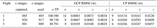
Table 3Summary statistics for each of the triangulations used to produce DSMs and ortho-mosaics from each of the three flight missions for ground control points (GCPs) and check points (CPs).
3.2.4 Derivation of snow depth
Snow depth was derived by differencing DSM of flights 2 and 3 from the baseline obtained during flight 1 (ref) as follows:
Equation (6) provides a map of difference between the two DSMs, henceforth referred to as the dDSM (after Nolan et al., 2015). Values of the dDSM are considered to represent snow depth, with the associated uncertainty considered in Sect. 3.3.
3.3 Quality and accuracy assessment
Summary statistics, typically based on the rms error of GCPs and CPs from the AT, indicate the expected accuracy of deliverables. Since snow depth is determined by differencing two DSMs, error propagation can provide an assessment of uncertainty associated with the dDSM. The overall accuracy of the DSM differencing approach should also be validated against independent reference data (e.g. snow depth measured in situ), temporally coincident with RPAS measurements. Areas of snow-free terrain during Flight 3 further supplement snow depth observations by providing an extensive source of samples with which to assess the repeatability of the photogrammetric modelling process.
Previous studies have considered the accuracy of RPAS-derived snow depth by comparison with reference data from in situ snow depth alone (Bühler et al., 2016; De Michele et al., 2016; Harder et al., 2016) while ignoring the uncertainty inherent to each photogrammetric model and their propagation into the dDSM. Here, the accuracy of photogrammetrically derived snow depth is assessed by exploring both approaches. Relating photogrammetric model quality, as inferred from GCPs and CPs, to observed uncertainties in the determination of snow depth provides the basis for realistically informing uncertainties in snow depth from ongoing RPAS measurements. This in turn allows rigorous inferences about the evolution of snow depth to be made, without the need for further campaigns of in situ validation. While high-resolution reference elevation data, such as lidar-derived elevation or surface models would provide a useful benchmark for assessing RPAS DSM quality, no such data were available for the study area.
3.3.1 Uncertainty associated with RPAS-derived snow depth
Since snow depth is determined via DSM differencing as a linear combination of two independently measured variables (Eq. 6), the uncertainty associated with snow depth (SD), measured in the vertical dimension, for each measurement date (n) can be obtained via Gaussian error propagation (James et al., 2012) as follows:
where ε for each DSM is the elevation error determined from the AT as the RMSEZ value for the set of CPs. Inherent in this simple approach is the assumption that the planimetric accuracy of each constituent DSM has negligible contribution to εdDSM. Calculating εdDSM provides a single estimate of uncertainty assumed to apply equally throughout the map of RPAS-derived snow depth for each date. Under the assumption that errors are normally distributed and bias-free, the RMSEz derived from CPs identifies the standard deviation σz, allowing the 90 % confidence level of z to be determined as 1.65×σZ. In turn, inferences associated with uncertainties for elevation differences, εdDSM, also depend on the Gaussian assumption to provide the 90 % confidence level.
In reality, perfect co-registration between constituent DSMs and the Gaussian assumption are unwarranted. Subsequently, inferences associated with the evolution of snow depth may be compromised due to confidence intervals being conservative or immoderate. Therefore, we use dDSM for snow-free areas to characterise the experimental distribution of errors and assess the validity of the Gaussian assumption in this context.
3.3.2 Validation against reference snow depth measurements
The approach above provides a means to determine the expected accuracy of snow depth derived from RPAS photogrammetric surveys. In order to validate this estimate, a reference data set of in situ observations was sampled in the field using snow probes, with a nominal precision of ±0.01 m, as described in Sect. 3.1.4. De Michele et al. (2016) assessed the accuracy of RPAS-derived snow depths against snow depth surfaces interpolated from 12 point measurements. This approach, however, may be limited by an inability to accurately resolve the spatial variability of snow depth, as well as the compounding effects of uncertainty associated with the interpolation scheme, particularly beyond the domain defined by the measured points.
Here, 430 measurements of snow depth provided 86 mean reference values, with the standard deviation of each set of five measurements providing 95 % confidence intervals. The aim of this sampling strategy was to assess and account for co-location uncertainty and spatial variability between the RPAS and reference snow depth data sets. Reference snow depths were compared with those from the spatially coincident pixels from the map of RPAS-derived snow depth. RPAS-derived snow depth quality was assessed in terms of residuals and weighted linear regression between reference and RPAS-derived snow depths.
3.3.3 Repeatability of photogrammetric modelling
Emergence of snow-free areas at the time of the spring flight facilitated comparison between autumn and spring DSMs on those areas. As the same terrain surface mapped from two independent flights should yield identical DSMs, the residual between them provides a means to characterise the distribution of errors in the photogrammetric processing, which can be readily compared to the assessment made from CPs.
Snow-covered and snow-free areas were segmented using an unsupervised classification of the spring ortho-image using the Iso Cluster classification tool in ArcGIS v10.3. With five output classes, this approach enabled discrimination between illuminated snow pixels, shaded snow pixels, and vegetation and soil-dominated snow-free pixels. Snow-free pixel classes were then grouped to provide a mask within which the distribution of spring dDSM values could be characterized. While this approach relies on the characterisation of repeatability for snow areas, good image contrast and the high overall density of TPs generated across the image block, regardless of the presence or absence of snow, indicates that photogrammetric reconstruction performance should be comparable for both snow-free and snow-covered areas. This is a product of the camera properties, which maintain high dynamic range across scenes of mixed land cover and extensive snow cover. Therefore, this residual represents a measure of the repeatability of the technique for measuring surface height change, including derivation of snow depth.

Figure 3Processed ortho-mosaics for autumn (a), winter (b) and spring (c) flights, with corresponding autumn hill-shaded DSM (d) and maps of snow depth derived for winter (e) and spring (f).
3.3.4 Resolution of fine-scale spatial variability
A primary motivation for exploring the use of RPAS photogrammetry for mapping a snowpack is the ability to resolve fine-scale spatial variability in snow depth. This capability was assessed by computing and comparing the semi-variograms of reference and RPAS-derived snow depths from the autumn flight. While the sample size for reference snow depths remained fixed (n=86), the semi-variogram of RPAS-derived snow depths could be calculated from many more samples. Two random samples were extracted from the spring dDSM map (n=1000 and n=5000), each yielding a semi-variogram capturing the spatial variability of snow depth with increasing detail, which were compared to that of the in situ observations.
4.1 Photogrammetric processing
4.1.1 Quality of the triangulation
Since GCPs are used to solve the photogrammetric model, they do not provide an independent assessment of accuracy. Such an assessment is provided by the CPs, the RMSE of which was of the order of centimetres for all flights (Table 3). Planimetric RMSE (i.e. x and y) was always substantially less than the GSD. Vertical RMSE (z) tended to be about double that achieved planimetrically but never exceeded 0.05 m. The final models were produced from a second and more constrained AT with all surveyed points used as GCPs, thus making the assessment conservative relative to the final products.
While the RMSE of CPs increased for the winter and spring flights, possibly due to a less constrained model, the level of accuracy achieved is compatible with expectations for the determination of snow depth. Additionally, the more tightly constrained first AT reduced the error for the baseline model, in turn contributing a reduced uncertainty in derived snow depths, despite the reduced control for subsequent ATs. For all flight missions, the photogrammetric processing performed well in the correlation of images and the construction of the image block, as indicated in Table 3. Tie point (TP) generation relies on the successful match of unique targets across multiple images, which was achieved despite the complicated contrast over snow. For all flights > 80 000, TPs were generated across the imaged area.
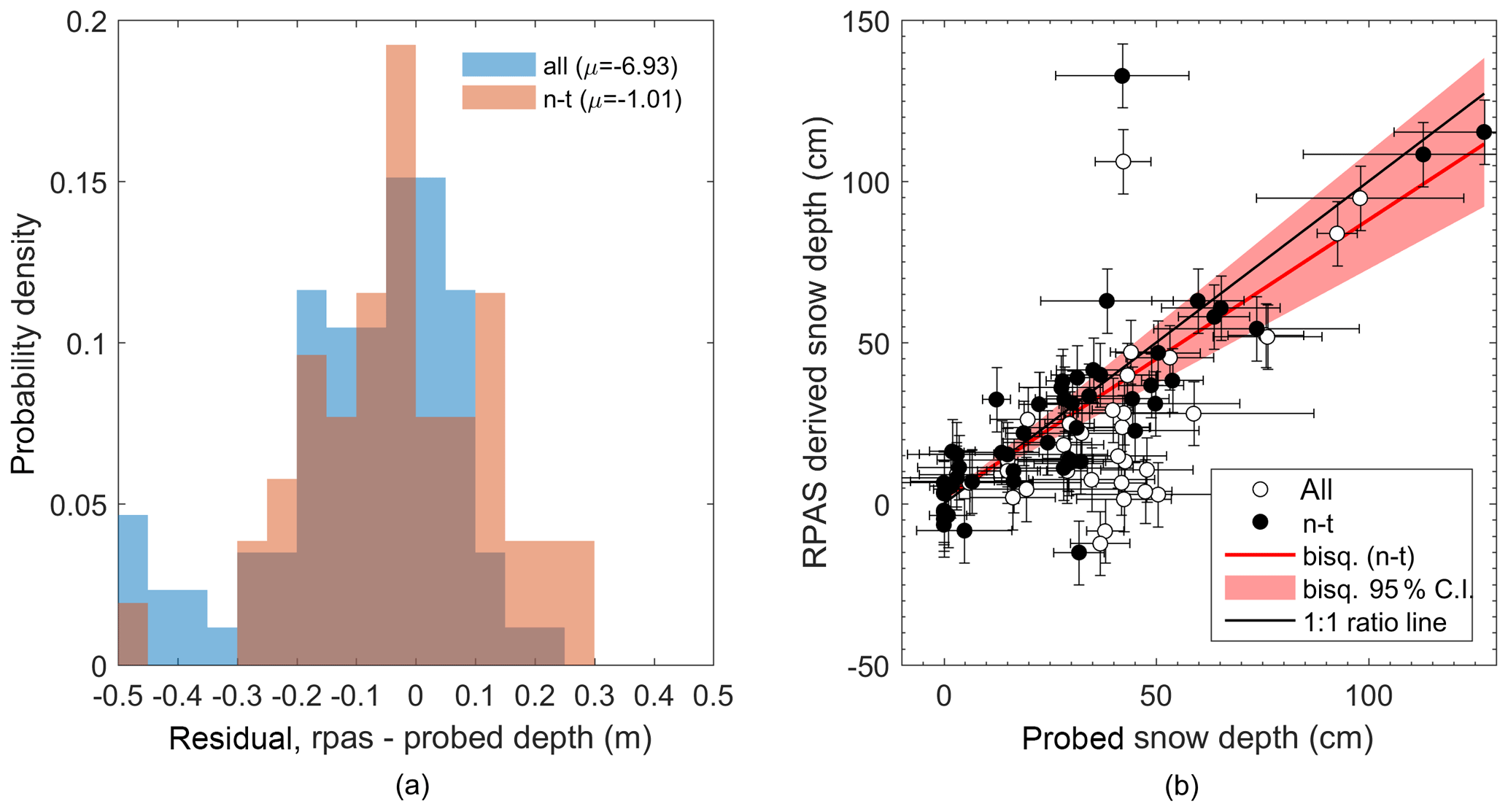
Figure 4Residuals between snow depths measured by RPAS photogrammetry and probing for all probe locations (“all”, blue) and non-tussock probe locations (“n-t”, red) (a), and bi-square (bisq.) weighted regression between snow depth derived from a 0.15 m RPAS grid and probed snow depths (b). Vertical error bars are determined from the error propagation associated with DSM differencing and have a magnitude of ±0.094 m, while horizontal error bars are calculated from the standard deviation of probe measurements made at each reference sampling location.
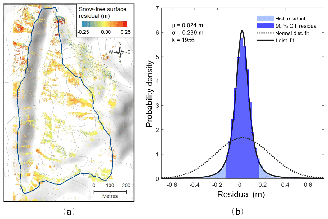
Figure 5Map (a) and histogram (b) of the vertical residual for snow-free areas for surface models derived from the autumn and spring flights. The histogram includes fitted normal and t location-scale (t) distributions.
4.1.2 Determination of snow depth
Snow depth was found to be highly variable across the study catchment for both winter and spring (Fig. 3). The midwinter flight mapped near-complete snow cover across the study catchment, while large snow-free areas developed by the spring flight, where snow-covered area was reduced by about one-third (Fig. 3a and b). Where snow was present, depths ranged from less than 0.10 m, typically on exposed ridgelines and broad elevated slopes, to 2 m or more where cornices formed along ridgelines, as well as in gullies. Average snow depth was greater for winter, although maximum depths were comparable between winter and spring. Between winter and spring, considerable ablation was observed. Areas of deepest snow were spatially coincident between winter and spring, with the greatest retention of snow in cornices and gullies. Where shallow snow was present on ridgelines in winter, it was largely lost by spring.
4.2 Accuracy assessment and validation of snow depth
4.2.1 Propagation of aero-triangulation error
Propagation of errors under the Gaussian assumption, based on the RMSE from each AT, yielded vertical uncertainties for snow depths at the 90 % confidence level of ±0.077 m for the winter flight and ±0.084 m for the spring flight. This one-dimensional approach to error propagation assumes that the planimetric geolocation of individual surfaces, and subsequently the co-registration of surface pairs, does not contribute significantly to the vertical uncertainty.
4.2.2 Assessment against reference probe data
Comparison of RPAS-derived and reference snow depth yielded a mean residual of −0.069 m, indicating that, on average, reference depths were greater than RPAS-derived depths. Filtering the reference data set to exclude reference measurements that were made in areas occupied by tussock (Chionochloa rigida) vegetation, however, improved the mean residual to −0.01 m (Fig. 4a). The small residual is indicative of good agreement between the two data sets while also indicating that, overall, snow depths measured by probing may be overestimated. Limitations of probing and uncertainty introduced due to the presence of vegetation is discussed further in Sect. 5.2.1.
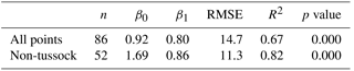
Good agreement between data sets is further demonstrated in Fig. 4b. Relatively large horizontal error bars accompanying the reference measurements (Fig. 4b) reflect the substantial spatial variability in snow depth measured by probing, even within arm's reach. Substantial departure occurs for reference snow depths between 0.20 and 0.60 m which tend to exceed RPAS measurements. Negative depths in the RPAS-derived data set is a product of co-registration uncertainty, particularly in areas where the surface model represents large vegetation or is influenced by rock outcrops, as well as spurious values from the constituent DSMs. Agreement between reference and RPAS-derived data sets improved with the removal of reference measurements made above tussocks. This filtering saw the R2 value improve by 22 %, while RMSE decreased by 23 % (Table 4). The 1 : 1 ratio line was contained within the 95 % confidence interval of the weighted (bi-square) regression between RPAS-derived and filtered reference snow depths. Some disagreement between RPAS derived and probed snow depths is likely due to the varying areas over which snow depth was sampled by the two techniques, and resulting spatial uncertainty in comparing the two data sets.
Table 4Parameters of weighted regression between reference and RPAS-derived snow depths.
4.2.3 Comparison of DSMs from independent RPAS flights
The emergence of snow-free areas for the September flight permitted a comparison of height derived on snow-free surfaces between the pre-winter and spring flights (Fig. 5). The small magnitude of the residuals, compatible with errors consistent with the uncertainty of the triangulation CPs, demonstrates the repeatability in the derivation of snow-free surfaces. Furthermore, the absence of any spatially structured trend in the distribution of the residual indicates robust photogrammetric modelling from the RPAS platform. At 0.15 m resolution, the snow-free pixels from the spring mission provided a large sample (n= 5 936 428). The mean residual (bias) detected with respect to the pre-winter DSM was 0.024 m (σ=0.239 m) (Fig. 5).
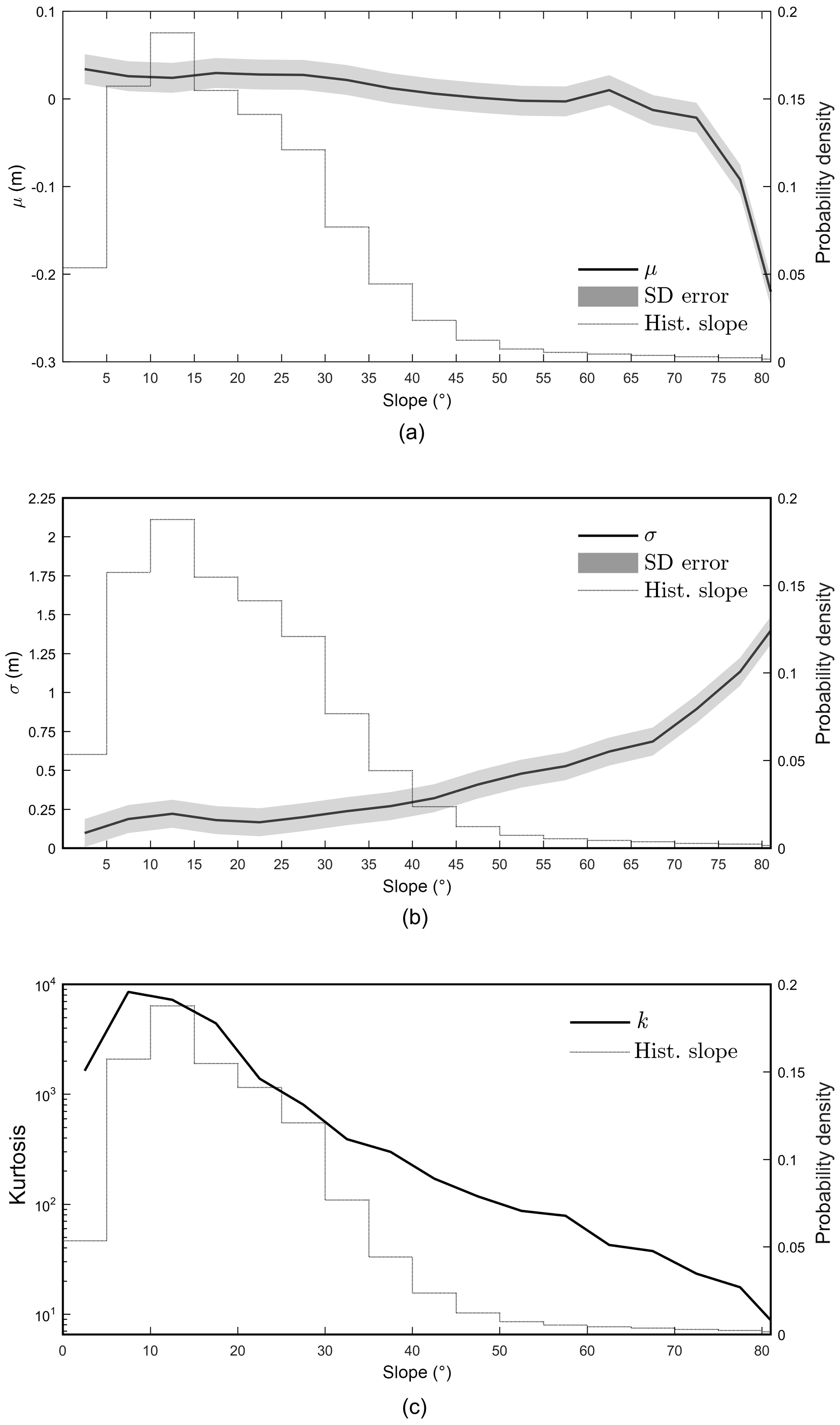
Figure 6Mean, μ (a), standard deviation, σ (b) and distribution kurtosis (c) for the residual, in terms of discrete classes of slope (5∘ width), up to the 90th percentile of slope. Kurtosis is plotted on a log-scale and is accompanied by a standard error of 606. The slope histogram has been clipped to the 90th percentile.
The set of residuals departed substantially from the Gaussian distribution and was better represented by the Student's t location-scale distribution (Fig. 6):
where μ, σ and v are the location, scale and shape parameters, respectively. Large kurtosis (calculated k=1956) associated with the histogram of residuals in Fig. 6 shows significant departure from a Gaussian law (for which k=3) of equal standard deviation, σ. The leptokurtic experimental distribution results in a narrower 90 % confidence interval than that estimated under the Gaussian assumption with σ=0.24 m, while the probability of large residuals is larger than predicted by a Gaussian distribution. Overall, the mean residual (μ=0.02 m) and the precision of ±0.14 m (90 % confidence level, calculated from the distribution 90th percentile; Fig. 6) exceeds the uncertainties estimated from error propagation alone (±0.08 m at 90 % confidence level; see Sect. 4.1.1) yet support the suitable repeatability of the photogrammetric modelling. Importantly, the significant departure from a normal distribution shows that assessing the variability from a Gaussian fit on stable targets (±0.39 m at the 90 % level) would significantly overestimate the confidence interval. On the other hand, the 90% confidence interval calculated from the fitted Student's t location-scale is ±0.10 m (Table 5). The significance of this result with respect to statistical inferences is discussed further in Sect. 5.2.2.
Table 5Observed (calculated under Gaussian assumption) and fitted normal and t location-scale (t l-s) parameters for the residual distributions shown in Fig. 5b.
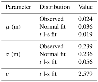
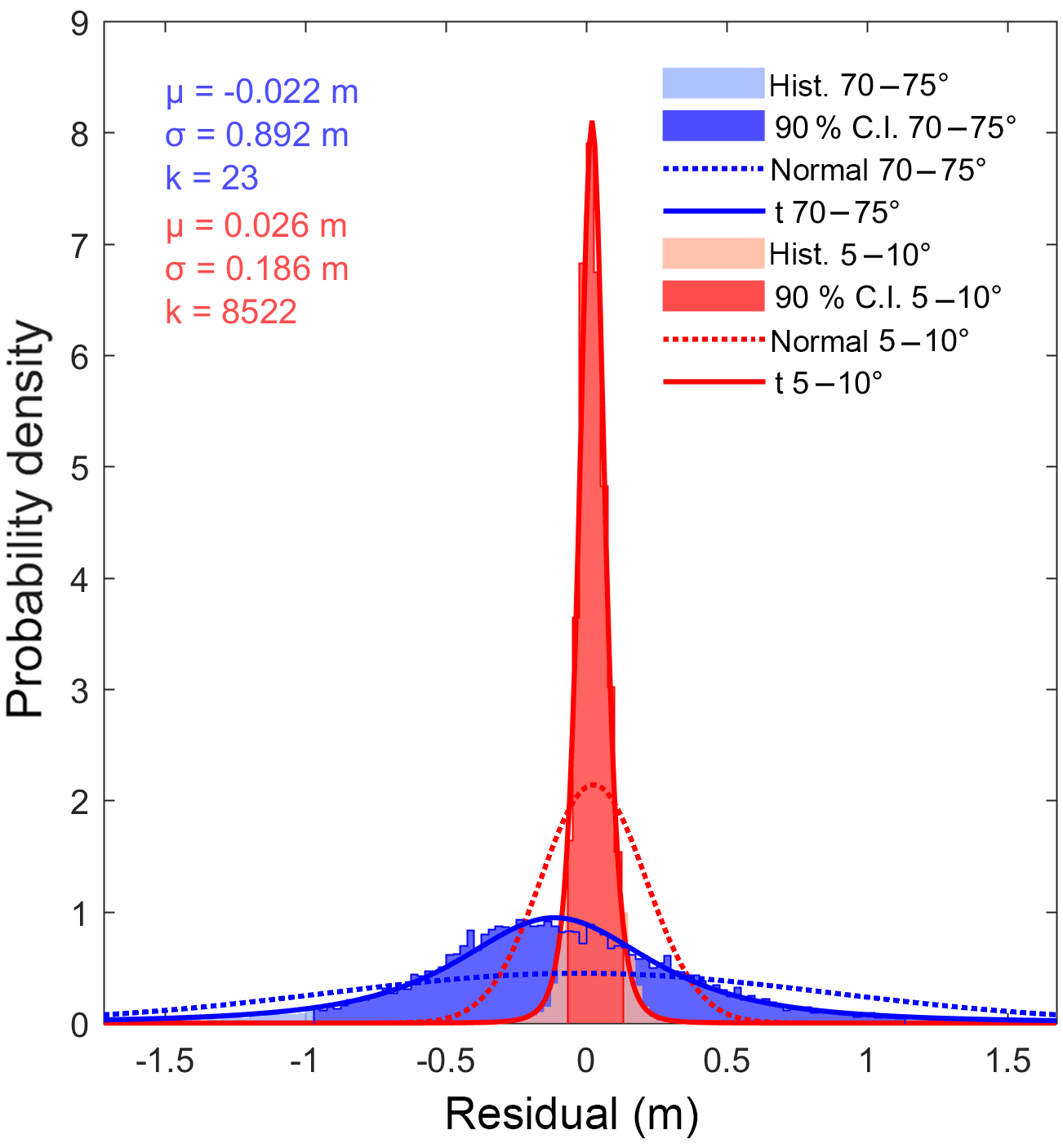
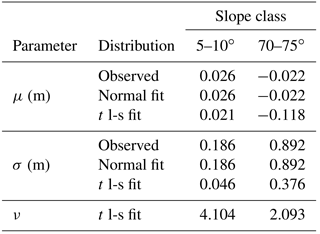
Figure 7Comparison of histograms and accompanying descriptive statistics for the residual between DSMs for slopes between 5 and 10∘ and slopes between 70 and 75∘. Flatter slopes are found to exhibit extreme kurtosis relative to steeper slopes. Normal and t location-scale (t) distributions are shown.
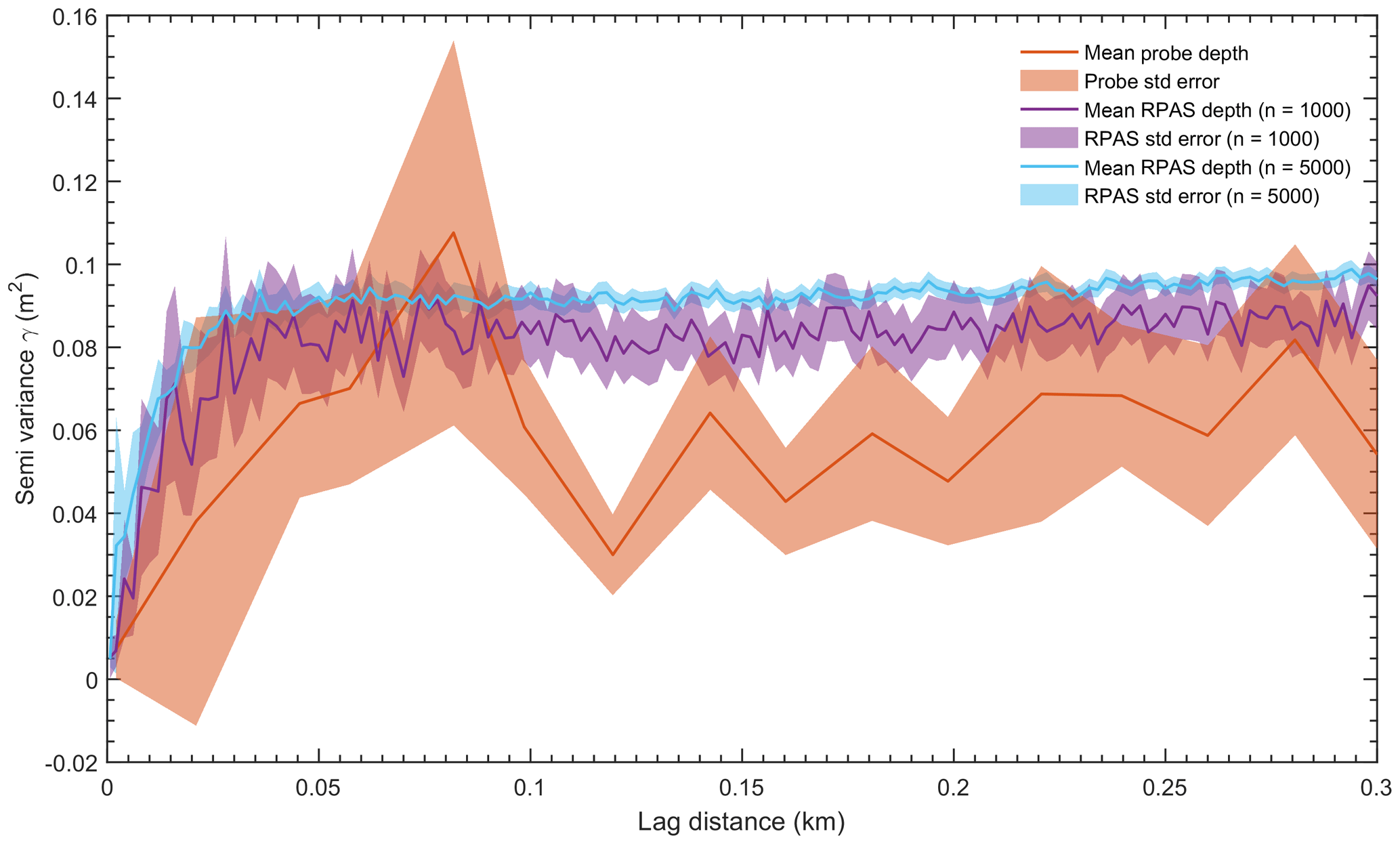
Figure 8Semi-variograms for snow depth, based on measurements provided by probing (86 samples), and two random samples drawn from RPAS-derived snow depth of 1000 and 5000 observations.
The non-Gaussian nature of the residual distribution deserves further scrutiny. Similar distributions have been identified for comparable repeatability assessments of photogrammetric dDSMs used for mapping snow depth (Nolan et al., 2015), but have not been explored in detail. Analysing the variability of the mean and standard deviation of the residual for discrete classes of slope, as well as the kurtosis of the residual distribution, provided insight into the role of terrain. For classes of slope up to 65∘ the mean residual remains within the standard error, before becoming increasingly negative for the remaining classes (Fig. 6). Standard deviation exhibits a similar trend, remaining largely within the overall standard error for slope classes up to 45∘, beyond which variability increases.
The observed pattern in the mean and standard deviation of the residual indicates that larger and more variable errors are associated with steeper slopes. Reduced kurtosis accompanying the error distribution on larger slopes (Fig. 6) reveals a tendency towards a Gaussian distribution of residuals as mean slope increases. Here, for slopes >50∘, kurtosis was reduced below 100, and for slopes >85∘, kurtosis was less than 10, approaching that of the normal distribution. Therefore, the statistical distribution of error, while non-normal, also varies significantly with terrain characteristics, as highlighted by the comparison of the residual histogram for discrete classes of slope (Fig. 7 and Table 6). Subsequently, the overall distribution of residuals (Fig. 5b) is the result of a convolution between non-normal distributions and the hypsometry of the area (i.e. area-elevation distribution).
Table 6Observed (calculated under Gaussian assumption) and fitted normal and t location-scale (t l-s) parameters for the residual distributions shown in Fig. 7.
4.2.4 Characterising the spatial variability of snow depth
The semi-variograms for RPAS-derived snow depth, compared to that from the reference measurements, are shown Fig. 8. They exemplify the new insight that high-resolution mapping provides into the spatial variability of snow depth. Both the 1000 and 5000 random point samples captured a comparable structure of spatial auto-correlation with a range of ca. 40 m. The 5000-point sample improved the resolution of the semi-variogram, with an improved signal-to-noise ratio. In contrast, the reference data, despite being demanding in fieldwork, performed poorly at capturing the spatial variability, as most measurements were separated by a minimum distance of 50 m. A lack of spatial auto-correlation in the reference data confirms a posteriori that probing samples could be assumed to be independent of each other, which is desirable for the accuracy assessment. Additionally, it also reveals that probing failed to capture most of the spatial structure of the snow depth field, thus stressing a limitation of this classical method to characterise the snowpack.
5.1 Performance of RPAS photogrammetry for resolving snow depth
Overall, RPAS photogrammetry is found to be suitable for determining snow depth via DSM differencing. Primarily, the achievement of uncertainties <0.14 m at the 90 % confidence level for derived snow depth, demonstrated empirically by the repeatability analysis (Fig. 5), provides a basis for useful data capture, and robust inferences and interpretations. The reported magnitudes of uncertainties account for the sources discussed further below, and compare favourably with other similar studies (Vander Jagt et al., 2015; Bühler et al., 2016; De Michele et al., 2016; Harder et al., 2016). Decimetre levels of uncertainty appear to be an emerging benchmark for snow depths measured by RPAS photogrammetry and also considered as standard for airborne lidar (Deems et al., 2013). In terms of comparisons with in situ data, Fig. 4 shows good agreement between RPAS and reference snow depth, and that RPAS photogrammetry performance improves as snow depth increases. At the same time, use of probed snow depths as references for validating such data can be compromised by the nature of the underlying vegetation.
Mapping snow depth continuously at 0.15 m resolution, across an entire hydrological catchment, represents a new contribution to the quantification and characterisation of spatial variability in snow depth on this scale, which is up to 2 orders of magnitude greater than many similar studies to date. Before considering the broader implications of this in terms of snow processes, uncertainty, limitations and pitfalls of the approach are considered.
5.2 Sources and nature of uncertainty
5.2.1 Vegetation
Vegetation contributes to uncertainty, particularly when validating RPAS-derived snow depths against reference snow depths. As described in Sect. 4.2.2, the agreement between RPAS-derived and probed snow depths improved substantially when areas of large tussock vegetation were excluded. It is likely that the presence of tussock introduces a bias into the snow depth measurement, whereby a probe may penetrate the tussock foliage, and possibly also a sub-vegetation void, before striking the ground surface. This is similar to the cavity effect highlighted for airborne lidar measurement of snow (Painter et al., 2016), and similar challenges have been documented by Vander Jagt et al. (2015). High-resolution dDSMs, on the other hand, resolve the vegetation surface, and so vegetation height is inherently better accounted for.
As identified by Nolan et al. (2015), photogrammetrically derived snow depths may also be affected by the compaction of vegetation below the snowpack, which may introduce an anomalous signal of surface height change, to the point of returning false negative snow depths. Correcting observed surface height change would not be straightforward, and is not possible with the data acquired within this study. The effects of vegetation compaction are likely to be greatest in the early winter. As grass typically does not rebound until after the complete removal of the winter snowpack, ongoing subsidence of vegetation below the snowpack through midwinter and spring is expected to be minimal. Ongoing future measurement of snow depth via surface differencing (regardless of the source of DSMs) will benefit from the development and incorporation of vegetation compaction and cavity models.
Ultimately, this study suggests that, for areas dominated by tussock vegetation, RPAS photogrammetry may provide a more reliable means of measurement than probing. A lack of knowledge regarding the specific location of sub-snow vegetation when making measurements by probing is likely to provide a systematic overestimation of snow depth (Fig. 4). In the New Zealand context, almost all seasonal snow occurs above the treeline, so the inability of photogrammetry to penetrate the forest canopy is a lesser concern than for the Northern Hemisphere.
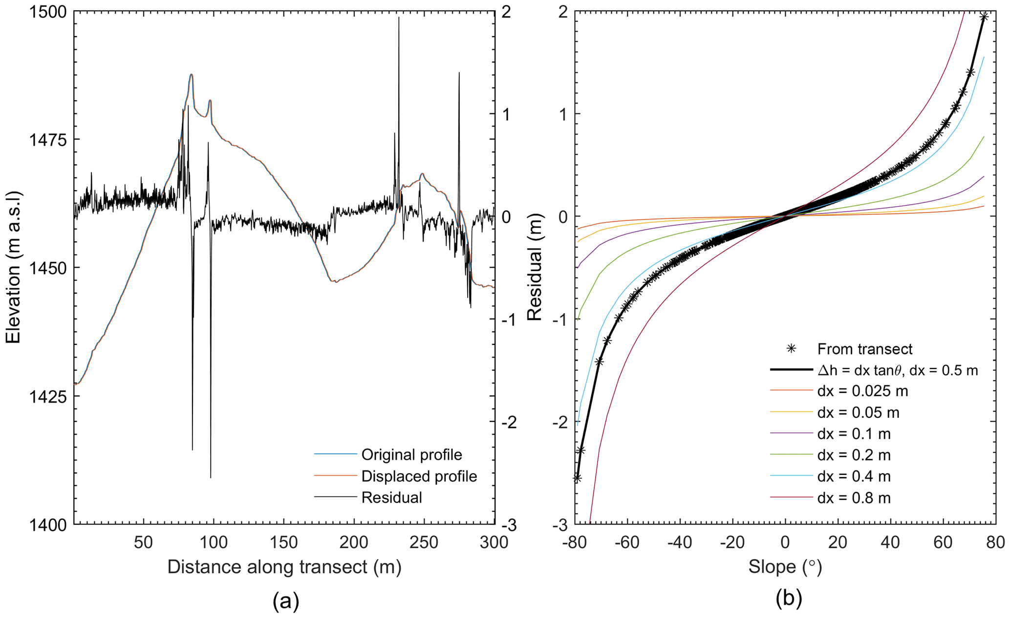
Figure 9The vertical residual between two elevation profiles, extracted from the same DSM, along a common transect and offset horizontally by 0.5 m (a), and the resulting residuals plotted as a function of terrain surface slope, for the applied offset of 0.5 m, and a range of other offsets (dx) (b).
5.2.2 Geolocation and co-registration
In mapping snow depth across a catchment with relatively complex terrain, we have been able to characterise the influence of terrain on dDSM uncertainty. The assumption that error associated with physical measurements is normally distributed and often underpins subsequent statistical inferences. As demonstrated in Sect. 4.2.3, the error associated with the bias between independently acquired DSMs significantly departed from normal and was better approximated by the Student's t location-scale distribution. This extremely leptokurtic distribution of residuals reflects the influence of relatively low frequency, but high-magnitude residuals beyond the probability of the normal law, despite an overall dominance of residuals about and close to the mean. A possible source of large residuals between two DSMs is their relative planimetric accuracy and subsequent co-registration quality (Kääb, 2005). For steep terrain in particular, a horizontal displacement between DSMs could add a component to dDSM uncertainty beyond the vertical accuracy of constituent DSMs. The residual (Δh) between two surface profiles, which are identical but horizontally displaced by 0.5 m, is shown in Fig. 9a. The error introduced to DSM differencing resulting from co-registration uncertainty increases with steepening slope. Maximum residuals coincide with the steepest terrain (near-vertical areas associated with rock outcrops) and exceed 2 m. The sign of the error is aspect dependent, assuming a uniform horizontal displacement.
Consistent with Kääb (2005), the vertical error introduced by a uniform, one-dimensional (e.g. horizontal) offset, is given by the following:
where dx is the offset between transects (i.e. 0.5 m in this case), and θ is the surface slope in degrees, as seen in Fig. 9b. It is clear from Fig. 9b that where the average slope of target surfaces is low and co-registration quality is good, the error introduced to a dDSM as a product of co-registration will be minimal. Increasing slope and/or co-registration uncertainty is accompanied by increased vertical uncertainty in the dDSM. This relationship is consistent with the findings of Sect. 4.2.3, resulting in the distribution of residuals departing substantially from the Gaussian distribution when the proportion of steep slopes is low. These findings provide context for the effect noted by Nolan et al. (2015), whereby a non-normal distribution of residuals associated with photogrammetric mapping of snow depth was found to narrow further when the area considered was restricted to a frozen lake (i.e. near planar) surface.
Complicating this effect is the fact that co-registration uncertainty exists in two dimensions. Subsequently, it will become dependent on aspect as well as slope (Nuth and Kääb, 2011), with neither possessing a uniform spatial distribution. This effect is expected to be more pronounced with very high-resolution (i.e. sub-metre) surface models due to a greater frequency and magnitude of breaks in surface slope being resolved compared to coarser models. The modification of surface slope for constituent DSMs (e.g. through the addition of snow) further convolves the propagation of vertical uncertainty. Despite this, the leptokurtic observed error distribution indicates that the reliance on statistics that assume a Gaussian distribution of errors will provide an overestimated characterisation of the expected accuracy. Overestimation of uncertainties may in turn affect statistical inferences and the computation of uncertainties on derived parameters.
The convolution of vertical and planimetric accuracy stresses the importance of ensuring a robust AT and the benefits of utilising high-quality ground control. With new photogrammetric platforms leveraging non-metric cameras and resulting image blocks prone to suboptimal photogrammetric modelling (Sirguey et al., 2016), there is a need to be wary of systematic bias or spatial structure in the distribution of errors, which may not be revealed readily by residuals from the AT alone. These considerations are especially important where a relatively high level of precision is required, and the signal-to-noise ratio may be low when assessing relatively subtle surface height and/or volume changes from dDSMs. Utilising independent ATs as the control of co-registration quality, rather than explicitly co-registering DSMs, has the further advantage of simplifying the processing chain from data acquisition to change detection, mitigating against the risk of introducing gross error when co-registering DSMs and avoiding the need for snow-free (or stable) reference areas within the analysis region.
5.3 Pitfalls and limitations of RPAS photogrammetry
Initial processing using the photogrammetry module of Trimble Business Center (v3.40) produced strong striping artefacts in the dDSM. Striping involved a periodic bias in surface height change, aligned with the 15 image strips. This was readily revealed because identical flight plans between successive surveys made constructive errors obvious, rather than convoluted with terrain variability. This systematic error was severe and problematic, particularly when considering the surface change resulting from the addition of snow cover to the ground. Extensive snow cover concealed stable references, precluding characterisation of the error and its empirical removal from the real signal of surface height change (e.g. Albani and Klinkenberg, 2003; Berthier et al., 2007). Products derived using UAS Master (v8.0) did not exhibit such artefacts, allowing the potential source of error associated with AT from TBC to be investigated.
The absence of systematic bias in dDSMs derived using UAS Master indicates a more reliable AT. Thus, the UAS Master triangulation provided a reference surface for further exploration of the nature of the bias propagated in the TBC triangulation. Comparisons from the winter flight are presented here. The nature of the photogrammetric problem described in Sect. 3.2.1 dictates that small errors in the interior orientation and/or the rotational components of the exterior orientation can result in large, spatially structured errors in the adjusted image block (Sirguey et al., 2016).
Cimoli et al. (2017) reported an improved performance in mapping snow depth with the application of a radial lens distortion correction. In our case, no significant difference was detected between the distortion models provided for each of the two software calibrations of the same camera, for the same flight. (Fig. 11a). Minimal divergence in lens distortion was observed beyond 10 mm radius, reaching 1 % at 14.5 mm. Agreement between lens distortion models indicated that differing interior orientation solutions between TBC and UAS Master were not the source of the artefacts seen in products of the TBC triangulation.
Since the observed artefact was propagated along the flight lines, the roll parameter (ω) was considered. Bias in the estimation of this parameter could lead to a systematic elevation offset of resected points between flight lines, either raising or lowering the terrain, as documented in the case of stereo-satellite imagery by Berthier et al. (2007). Occurrence of this for multiple flights with near-identical flight lines would exacerbate constructive biases, resulting in the striping in the dDSM. Alternatively, pitch and yaw parameters are unlikely to produce such an artefact along the flight direction (Ebner and Fritz, 1980). The residual of ω for individual photo centres between each of the two software packages confirmed that a positive bias existed in the ω value as estimated by TBC v3.40 relative to that provided by UAS Master. The mean residual () was found to be 0.014∘.
The impact of bias in ω on the resected height h for a target with respect to a photo centre can be estimated simply as a right-angled triangle, since values of ω are small compared to the baseline length, l, which is equal to half the distance between adjacent flight lines (see Fig. 12):
Using the observed value of 0.014∘ for , Δh was calculated for a range of typical values of h, yielding the relationship between h and Δh as shown in Fig. 11b. Bias in the estimation of the ω parameter during the AT can introduce a significant vertical error, dependent (non-linearly) on flying height (h), propagating an error of ±0.12 m at a flying height of 110 m. The increase in error with flying height above ground level was consistent with the observed propagation of striping artefacts in DSM products, whereby the magnitude of the observed bias decreased as terrain height increased (Fig. 10), while absolute flying height remained approximately constant.
The observed propagation reinforces the need for vigilance when working with such data sets, particularly those delivered from “off the shelf” photogrammetry packages, which are becoming increasingly popular. Artefacts such as the striping identified here, and evidence of non-optimal AT, are likely to be less obvious as the complexity of the mapped terrain increases. As RTK GPS-equipped RPAS become more common, increased precision of initial AT parameters may mitigate the risk of error introduced by spurious solutions for refined parameters. Currently, however, RTK systems have an increased power demand, which can substantially reduce the flight time.
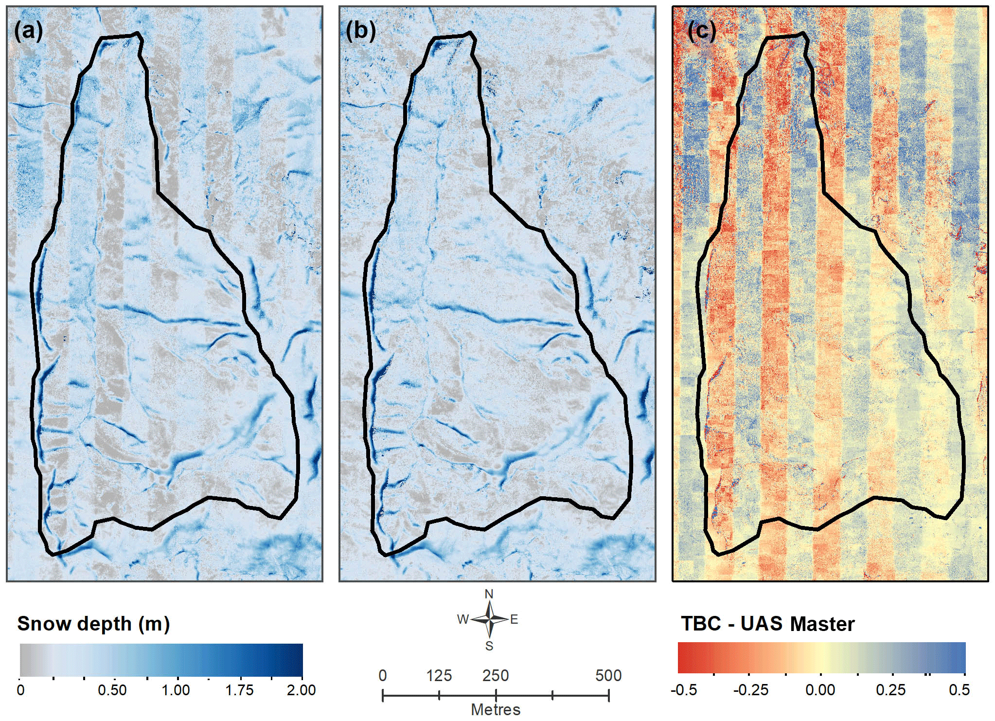
Figure 10Map of the systematic artefacts in surface height change (dh) (expected to represent snow depth), propagated when differencing digital surface models (DSMs) resulting from aerial-triangulation in TBC v3.40 (a) compared with the dDSM from UAS Master (b). Vertical (north–south aligned) striping is highlighted in (c), which shows the residual between dDSMs derived from TBC and UAS Master.
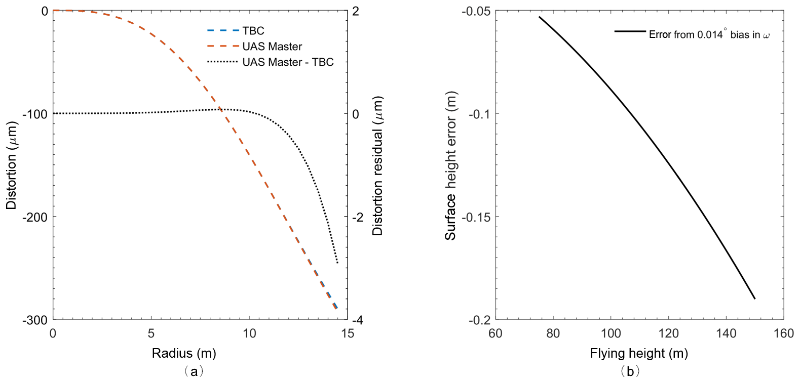
Figure 11Comparison of lens distortion characterised by individual triangulations of data from the same flight carried out in two different software packages, TBC and UAS Master (a), and the error in surface height propagated by a bias in the roll parameter, ω, in relation to flying height (b). The distortion residual was only apparent at radial distances >12 mm (a), while the observed mean bias in ω that was propagated by TBC results in substantial errors in surface height (b).
5.4 Spatial and temporal trends in snow cover
Figure 8 demonstrates the new insight that RPAS photogrammetry can provide over probing for resolving spatial variability in snow depth, particularly on fine scales. Therefore, RPAS photogrammetry can provide a basis for improving spatially distributed snowpack models. In turn, this contribution will further improve understanding of seasonal snow processes, where there has been a dependency on point-based observations over glaciers to characterise atmospheric controls on seasonal snow (e.g. Cullen and Conway, 2015). While knowledge of the atmospheric controls on ablation processes has improved (Conway and Cullen, 2016), our understanding of the redistribution of snow and preferential accumulation have not kept pace. RPAS photogrammetry represents a valuable avenue for determining how these processes are represented in existing and new snow and glacier models, which will enable short-term hydrological forecasts and climate projections in snow-covered areas to be improved. Such data can also facilitate the use of geostatistical approaches for examining controls on spatial distribution of snow, such as that applied to the Brewster Glacier, New Zealand (Cullen et al., 2017). In this case, the density of measurements provides insights into spatial variability on scales that would allow consideration of terrain and meteorological controls on snow distribution on micro-scales, extending understanding beyond the spatial co-variance between snow depth and elevation.
The ability to resolve fine-scale variability reliably from continuous raster snow maps lessens the dependence on interpolation through areas of sparse data for interpreting controls on spatial distribution of snow. While previous studies have been able to correlate between snow and terrain properties (e.g. Anderson et al., 2014), such studies rely on the inference of catchment-scale processes from transect-scale observations. The ability to produce spatially continuous maps of snow depth across an entire catchment at a resolution of 0.15 m bridges this gap and reduces the reliance on inferences when scaling up from point- or transect-based in situ observations to catchment-scale processes. Such data sets provide an opportunity to build on previous work in understanding the relationships between snow redistribution, preferential accumulation and ablation, terrain and meteorology (Winstral et al., 2002, 2013; Webster et al., 2015; Revuelto et al., 2016). While RPAS photogrammetry is severely limited in spatial scale compared to airborne lidar, resolving snow depth in this way across an entire catchment facilitates robust integration into hydrological models, enhanced by validation against catchment discharge (e.g. from streamflow data).

Figure 12Schematic of the relationship between height (h), baseline length (l) and the interior angle (θ) that may be affected by a bias (rθ) for a terrain point position resected from images centred at p1 and p2, when the mean bias () is small (e.g. 0.014∘ in this case).
The mapping of snow depth effectively provides a volumetric view of the snowpack across the catchment (i.e. depth × area). The snowpack mass balance in terms of SWE can be calculated based on in situ measurements of snow density. While snow depth was only determined for two dates in this case, emergent trends within the data can be explored. Between the winter and spring flights, the catchment snow-covered area (SCA) decreased from 100 % to 67 %. Bulk snowpack densities, measured gravimetrically at a single snow pit for the winter flight (314 kg m−3), and two snow pits for the spring flight (391 kg m−3), allow catchment SWE to be calculated, revealing a 20 % reduction in SWE between flights. This highlights the importance of effective concentration of snow in preferred areas, and the complex spatial distribution that results. The ability to detect this, even with a temporally limited data set, indicates the potential for RPAS photogrammetry as a measurement approach for improving resolution and understanding of snow hydrology. In particular, such data sets may offer a unique opportunity to assess the performance of models forced by remotely sensed data of coarser resolution in estimating SWE from estimates of subpixel fractional SCA (Bair et al., 2016).
This study has demonstrated that RPAS photogrammetry provides a suitable, repeatable means of reliably determining snow depth in an alpine catchment of low relief that possesses some terrain complexity. Achieving decimetre-level accuracy for measuring snow depth provides a basis for monitoring seasonal snowpacks and associated processes, especially considering the capacity to provide very high-resolution, spatially continuous measurements across an entire hydrological catchment. This ability to characterise the seasonal snowpack will provide an important stepping stone for improved modelling of seasonal snow and associated processes, especially through accurate mapping of an entire hydrological catchment.
Challenges encountered through this deployment provide important points for consideration in this and other applications of close-range photogrammetry, especially from RPAS platforms, for surface and volume change analysis. Specifically, a small but persistent bias in photogrammetric solutions for the roll parameter exemplifies the possibility of suboptimal solutions in processing software. Such a bias can introduce substantial systematic errors which may be difficult to correct and can compromise further analysis.
We show that uncertainty analysis from the AT only, based on a limited number of check points, may underestimate the uncertainty. Alternatively, an assessment of repeatability of photogrammetric modelling on stable ground can support a more detailed uncertainty analysis. It reveals, however, that the statistical distribution of the error of differentiated surface models is more complex than normal and governed by terrain parameters. The leptokurtic residual distribution demonstrates that an assumption of Gaussian law can substantially overestimate confidence intervals, in turn compromising inferences. This result has important practical applications for the computation of uncertainties in studies that characterise volume change from repeated surface modelling.
Finally, there is scope to further refine the characterisation of uncertainty associated with RPAS photogrammetry in order to ensure that all potential sources of error are captured, and that statistical analysis is appropriate to the distributions within underlying data. Existing methods for mitigating the impact of co-registration uncertainty of coarser products may permit modelling and correction of such errors in the very high-resolution products that are now available.
The data used in this research are available on request from Todd A. N. Redpath.
TR and PS designed the study and collected the data. TR processed and analysed the data and wrote the manuscript with input from PS and NC. PS and NC supervised the research.
The authors declare that they have no conflict of interest.
The authors are grateful to those who provided assistance in the field:
Julien Boeuf, Kelly Gragg, Mike Denham, Craig MacDonell, Aubrey Miller, Sam
West, Thomas Ibbotson and Alia Khan. Sean Fitzsimons provided helpful
feedback on the draft manuscript. This research was carried out under the
Department of Conservation Research & Collection Authorisation 53609-GEO.
This research was funded by a University of Otago Doctoral Scholarship with
support from the Department of Geography and an internal grant of the
National School of Surveying, as well as a fieldwork grant from the New
Zealand Hydrological Society. The authors thank the editor, Martin
Schneebeli, and two anonymous reviewers, whose thorough and thoughtful
comments improved this manuscript.
Edited by:
Martin Schneebeli
Reviewed by: two anonymous referees
Albani, M. and Klinkenberg, B.: A spatial filter for the removal of striping artifacts in digital elevation models, Photogramm. Eng. Remote, 69, 755–765, https://doi.org/10.14358/PERS.69.7.755, 2003.
Anderson, B. T., McNamara, J. P., Marshall, H.-P., and Flores, A. N.: Insights into the physical processes controlling correlations between snow distribution and terrain properties, Water. Resour. Res., 50, 4545–4563, https://doi.org/10.1002/2013WR013714, 2014.
Avanzi, F., Bianchi, A., Cina, A., De Michele, C., Maschio, P., Pagliari, D., Passoni, D., Pinto, L., Piras, M., and Rossi, L.: Centimetric accuracy in snow depth using unmanned aerial system photogrammetry and a multistation, Remote Sensing, 10, 1–16, https://doi.org/10.3390/rs10050765, 2018.
Bair, E. H., Rittger, K., Davis, R. E., Painter, T. H., and Dozier, J.: Validating reconstruction of snow water equivalent in California's Sierra Nevada using measurements from the NASA Airborne Snow Observatory, Water. Resour. Res., 52, 8437–8460, https://doi.org/10.1002/2016WR018704, 2016.
Berthier, E., Arnaud, Y., Kumar, R., Ahmad, S., Wagnon, P., and Chevallier, P.: Remote sensing estimates of glacier mass balances in the Himachal Pradesh (Western Himalaya, India), Remote Sens. Environ., 108, 327–338, https://doi.org/10.1016/j.rse.2006.11.017, 2007.
Bessho, K., Date, K., Hayashi, M., Ikeda, A., Imai, T., Inoue, H., Kumagai, Y., Miyakawa, T., Murata, H., Ohno, T., Okuyama, A., Oyama, R., Sasaki, Y., Shimazu, Y., Shimoji, K., Sumida, Y., Suzuki, M., Taniguchi, H., Tsuchiyama, H., Uesawa, D., Yokota, H., and Yoshida, R.: An Introduction to Himawari-8/9 – Japan's New-Generation Geostationary Meteorological Satellites, J. Meteorol. Soc. Jpn. Ser. II, 94, 151–183, https://doi.org/10.2151/jmsj.2016-009, 2016.
Brown, D. C.: Close-range camera calibration, Photogramm. Eng., 37, 855–866, 1971.
Bühler, Y., Adams, M. S., Bösch, R., and Stoffel, A.: Mapping snow depth in alpine terrain with unmanned aerial systems (UASs): potential and limitations, The Cryosphere, 10, 1075–1088, https://doi.org/10.5194/tc-10-1075-2016, 2016.
Bühler, Y., Adams, M. S., Stoffel, A., and Boesch, R.: Photogrammetric reconstruction of homogenous snow surfaces in alpine terrain applying near-infrared UAS imagery, Int. J. Remote Sens., 38, 3135–3158, https://doi.org/10.1080/01431161.2016.1275060, 2017.
Cimoli, E., Marcer, M., Vandecrux, B., Bøggild, C. E., Williams, G., and Simonsen, S. B.: Application of Low-Cost UASs and Digital Photogrammetry for High-Resolution Snow Depth Mapping in the Arctic, Remote Sens., 9, 1142, https://doi.org/10.3390/rs9111144, 2017.
Clark, M. P., Hendrikx, J., Slater, A. G., Kavetski, D., Anderson, B., Cullen, N. J., Kerr, T., Hreinsson, E. Ö., and Woods, R. A.: Representing spatial variability of snow water equivalent in hydrologic and land-surface models?: A review, Water. Resour. Res., 47, W07539, https://doi.org/10.1029/2011WR010745, 2011.
Conway, J. P. and Cullen, N. J.: Cloud effects on surface energy and mass balance in the ablation area of Brewster Glacier, New Zealand, The Cryosphere, 10, 313–328, https://doi.org/10.5194/tc-10-313-2016, 2016
Cullen, N. J. and Conway, J. P.: A 22 month record of surface meteorology and energy balance from the ablation zone of Brewster Glacier, New Zealand, J. Glaciol., 61, 931–946, https://doi.org/10.3189/2015JoG15J004, 2015.
Cullen, N. J., Anderson, B., Sirguey, P., Stumm, D., Mackintosh, A., Conway, J. P., Horgan, H. J., Dadic, R., Fitzsimons, S. J., and Lorrey, A.: An 11-year record of mass balance of Brewster Glacier, New Zealand, determined using a geostatistical approach, J. Glaciol., 63, 199–217, https://doi.org/10.1017/jog.2016.128, 2017.
Deems, J. S., Painter, T. H., and Finnegan, D. C.: Lidar measurement of snow depth: A review, J. Glaciol., 59, 467–479, https://doi.org/10.3189/2013JoG12J154, 2013.
De Michele, C., Avanzi, F., Passoni, D., Barzaghi, R., Pinto, L., Dosso, P., Ghezzi, A., Gianatti, R., and Della Vedova, G.: Using a fixed-wing UAS to map snow depth distribution: an evaluation at peak accumulation, The Cryosphere, 10, 511–522, https://doi.org/10.5194/tc-10-511-2016, 2016.
Dozier, J.: Spectral signature of alpine snow cover from the Landsat Thematic Mapper, Remote Sens. Environ., 22, 9–22, 1989.
Ebner, H. and Fritz, L.: Aerotriangulation, in: Manual of Photogrammetry, 4th edn., edited by: Slama, C. C., American Society of Photogrammetry, Falls Church, 453–518, 1980.
Fernandes, R., Prevost, C., Canisius, F., Leblanc, S. G., Maloley, M., Oakes, S., Holman, K., and Knudby, A.: Monitoring snow depth change across a range of landscapes with ephemeral snow packs using Structure from Motion applied to lightweight unmanned aerial vehicle videos, The Cryosphere Discuss., https://doi.org/10.5194/tc-2018-82, in review, 2018.
Hall, D. K., Crawford, C. J., Di Girolamo, N. E., Riggs, G. A., and Foster, J. L.: Detection of earlier snowmelt in the Wind River Range, Wyoming, using Landsat imagery, 1972–2013, Remote Sens. Environ., 162, 45–54, https://doi.org/10.1016/j.rse.2015.01.032, 2015.
Hall, D. K., Riggs, G. A., Salomonson, V. V, Di Girolamo, N. E., and Bayr, K. J.: MODIS snow-cover products, Remote Sens. Environ., 83, 181–194, https://doi.org/10.1016/S0034-4257(02)00095-0, 2002.
Harder, P., Schirmer, M., Pomeroy, J., and Helgason, W.: Accuracy of snow depth estimation in mountain and prairie environments by an unmanned aerial vehicle, The Cryosphere, 10, 2559–2571, https://doi.org/10.5194/tc-10-2559-2016, 2016.
Hirschmuller, H.: Accurate and efficient stereo processing by semi-global matching and mutual information, IEEE. T. Pattern Anal., 2, 807–814, https://doi.org/10.1109/CVPR.2005.56, 2008.
James, L. A., Hodgson, M. E., Ghoshal, S., and Latiolais, M. M.: Geomorphic change detection using historic maps and DEM differencing: The temporal dimension of geospatial analysis, Geomorphology, 137, 181–198, https://doi.org/10.1016/j.geomorph.2010.10.039, 2012.
Kääb, A.: Remote Sensing of Mountain Glaciers and Permafrost Creep. Zürich: Geographisches Institut der Universiturich, Zürich, 2005.
Kerr, T., Clark, M., Hendrikx, J., and Anderson, B.: Snow distribution in a steep mid-latitude alpine catchment, Adv. Water Resour., 55, 17–24, https://doi.org/10.1016/j.advwatres.2012.12.010, 2013.
Kinar, N. J. and Pomeroy, J. W.: Measurement of the physical properties of the snowpack, Rev. Geophys., 53, 481–544, https://doi.org/10.1002/2015RG000481, 2015.
Lemmetyinen, J., Derksen, C., Rott, H., Macelloni, G., King, J., Schneebeli, M., Wiesmann, A., Leppänen, L., Kontu, A., and Pulliainen, J.: Retrieval of Effective Correlation Length and Snow Water Equivalent from Radar and Passive Microwave Measurements, Remote Sens., 10, 170, https://doi.org/10.3390/rs10020170, 2018.
Lindeberg, T.: Image Matching Using Generalized Scale-Space Interest Points, J. Math. Imaging Vis., 52, 3–36, https://doi.org/10.1007/s10851-014-0541-0, 2015.
Linder, W.: Digital Photogrammetry: A Practical Course, 4th edn., Heidelberg, Springer, 2016.
Malenovský, Z., Rott, H., Cihlar, J., Schaepman, M. E., García-Santos, G., Fernandes, R., and Berger, M.: Sentinels for science: Potential of Sentinel-1, -2, and -3 missions for scientific observations of ocean, cryosphere, and land, Remote Sens. Environ., 120, 91–101, https://doi.org/10.1016/j.rse.2011.09.026, 2012.
Mankin, J. S., Viviroli, D., Singh, D., Hoekstra, A. Y., and Diffenbaugh, N. S.: The potential for snow to supply human water demand in the present and future, Environ. Res. Lett., 10, 114016, https://doi.org/10.1088/1748-9326/10/11/114016, 2015.
Marti, R., Gascoin, S., Berthier, E., de Pinel, M., Houet, T., and Laffly, D.: Mapping snow depth in open alpine terrain from stereo satellite imagery, The Cryosphere, 10, 1361–1380, https://doi.org/10.5194/tc-10-1361-2016, 2016.
Nolan, M., Larsen, C., and Sturm, M.: Mapping snow depth from manned aircraft on landscape scales at centimeter resolution using structure-from-motion photogrammetry, The Cryosphere, 9, 1445–1463, https://doi.org/10.5194/tc-9-1445-2015, 2015.
Nolin, A. W. and Dozier, J.: Estimating snow grain size using AVIRIS data, Remote Sens. Environ., 44, 231–238, https://doi.org/10.1016/0034-4257(93)90018-S, 1993.
Nuth, C. and Kääb, A.: Co-registration and bias corrections of satellite elevation data sets for quantifying glacier thickness change, The Cryosphere, 5, 271–290, https://doi.org/10.5194/tc-5-271-2011, 2011.
Painter, T. H., Berisford, D. F., Boardman, J. W., Bormann, K. J., Deems, J. S., Gehrke, F., Hedrick, A., Joyce, M., Laidlaw, R., Marks, D., Mattmann, C., McGurk, B., Ramirez, P., Richardson, M., Skiles, S. M. K., Seidel, F. C., and Winstral, A.: The Airborne Snow Observatory: Fusion of scanning lidar, imaging spectrometer, and physically-based modeling for mapping snow water equivalent and snow albedo, Remote Sens. Environ., 184, 139–152, https://doi.org/10.1016/j.rse.2016.06.018, 2016.
Revuelto, J., Vionnet, V., López-Moreno, J. I., Lafaysse, M., and Morin, S.: Combining snowpack modeling and terrestrial laser scanner observations improves the simulation of small scale snow dynamics, J. Hydrol., 533, 291–307, https://doi.org/10.1016/j.jhydrol.2015.12.015, 2016.
Rittger, K., Painter, T. H., and Dozier, J. : Assessment of methods for mapping snow cover from MODIS, Adv. Water Resour., 51, 367–380, https://doi.org/10.1016/j.advwatres.2012.03.002, 2013.
Roy, D. P., Wulder, M. A., Loveland, T. R., C.E., W., Allen, R. G., Anderson, M. C., Helder, D., Irons, J. R., Johnson, D. M., Kennedy, R., Scambos, T. A., Schaaf, C. B., Schott, J. R., Sheng, Y., Vermote, E. F., Belward, A. S., Bindschadler, R., Cohen, W. B., Gao, F., Hipple, J. D., Hostert, P., Huntington, J., Justice, C. O., Kilic, A., Kovalskyy, V., Lee, Z. P., Lymburner, L., Masek, J. G., McCorkel, J., Shuai, Y., Trezza, R., Vogelmann, J., Wynne, R. H., and Zhu, Z.: Landsat-8: Science and product vision for terrestrial global change research, Remote Sens. Environ., 145, 154–172, https://doi.org/10.1016/j.rse.2014.02.001, 2014.
Sims, C. and Orwin, J. F.: Snowmelt generation on a hydrologically sensitive mountain range, Pisa Range, Central Otago, New Zealand, J. Hydrol., 50, 383–405, 2011.
Sirguey, P., Boeuf, J., Cambridge, R., and Mills, S.: Evidence of sub-optimal photogrammetric modelling in RPAS-based aerial surveys, in: Proceedings of the GeoCart'2016 and ICA Symposium on Cartography, edited by: Moore, A. and Drecki, I., New Zealand Cartographic Society Inc., 91–98, 2016.
Sirguey, P., Mathieu, R., and Arnaud, Y.: Subpixel monitoring of the seasonal snow cover with MODIS at 250 m spatial resolution in the Southern Alps of New Zealand: Methodology and accuracy assessment, Remote Sens. Environ., 113, 160–181, https://doi.org/10.1016/j.rse.2008.09.008, 2009.
Sturm, M., Goldstein, M. A., and Parr, C.: Water and life from snow: A trillion dollar science question, Water. Resour. Res., 53, 3534–3544, https://doi.org/10.1002/2017WR020840, 2017.
Treichler, D. and Kääb, A.: Snow depth from ICESat laser altimetry – A test study in southern Norway, Remote Sens. Environ., 191, 389–401, https://doi.org/10.1016/j.rse.2017.01.022, 2017.
Trimble: UAS Master 7.0: Tutorial, Trimble Germany, 2015.
Trimble: Release Notes for UASMaster 8.0.0, Trimble Navigation Limited, 2016.
Vander Jagt, B., Lucieer, A., Wallace, L., Turner, D., and Durand, M.: Snow depth retrieval with UAS using photogrammetric techniques, Geosciences, 5, 264–285, https://doi.org/10.3390/geosciences5030264, 2015.
Watts, A. C., Ambrosia, V. G., and Hinkley, E. A.: Unmanned aircraft systems in remote sensing and scientific research: Classification and considerations of use, Remote Sens., 4, 1671–1692, https://doi.org/10.3390/rs4061671, 2012.
Webster, C. S., Kingston, D. G., and Kerr, T.: Inter-annual variation in the topographic controls on catchment-scale snow distribution in a maritime alpine catchment, New Zealand, Hydrol. Process., 29, 1096–1109, https://doi.org/10.1002/hyp.10224, 2015.
Winstral, A., Elder, K., and Davis, R. E.: Spatial Snow Modeling of Wind-Redistributed Snow Using Terrain-Based Parameters, J. Hydrometeorol., 3, 524–538, https://doi.org/10.1175/1525-7541(2002)003<0524:SSMOWR>2.0.CO;2, 2002.
Winstral, A. and Marks, D.: Long-term snow distribution observations in a mountain catchment: Assessing variability, time stability, and the representativeness of an index site, Water. Resour. Res., 50, 293–305, https://doi.org/10.1002/2012WR013038, 2014.
Winstral, A., Marks, D., and Gurney, R.: Simulating wind-affected snow accumulations at catchment to basin scales, Adv. Water Resour., 55, 64–79, https://doi.org/10.1016/j.advwatres.2012.08.011, 2013.