Consumption of atmospheric methane by the Qinghai–Tibet Plateau alpine steppe ecosystem

The methane (CH₄) cycle on the Qinghai–Tibet Plateau (QTP), the world's largest high-elevation permafrost region, is sensitive to climate change and subsequent freezing and thawing dynamics. Yet, its magnitudes, patterns, and environmental controls are still poorly understood. Here, we report results from five continuous year-round CH₄ observations from a typical alpine steppe ecosystem in the QTP permafrost region. Our results suggest that the QTP permafrost region was a CH₄ sink of $-\mathrm{0.86}\pm \mathrm{0.23}$ g CH₄-C m⁻² yr⁻¹ over 2012–2016, a rate higher than that of many other permafrost areas, such as the Arctic tundra in northern Greenland, Alaska, and western Siberia. Soil temperature and soil water content were dominant factors controlling CH₄ fluxes; however, their correlations changed with soil depths due to freezing and thawing dynamics. This region was a net CH₄ sink in autumn, but a net source in spring, despite both seasons experiencing similar top soil thawing and freezing dynamics. The opposite CH₄ source–sink function in spring versus in autumn was likely caused by the respective seasons' specialized freezing and thawing processes, which modified the vertical distribution of soil layers that are highly mixed in autumn, but not in spring. Furthermore, the traditional definition of four seasons failed to capture the pattern of the annual CH₄ cycle. We developed a new seasonal division method based on soil temperature, bacterial activity, and permafrost active layer thickness, which significantly improved the modeling of the annual CH₄ cycle. Collectively, our findings highlight the critical role of fine-scale climate freezing and thawing dynamics in driving permafrost CH₄ dynamics, which needs to be better monitored and modeled in Earth system models.

1 Introduction

Since 2007, the global atmospheric methane concentration [CH₄] continues to rise, after remaining stable between the 1990s and 2006 (Rigby et al., 2008; IPCC, 2013; Patra and Kort, 2016). Understanding mechanisms for this recent increase requires improved knowledge of CH₄ sources and sinks for regional and global CH₄ budgets (Kirschke et al., 2013; Zona et al., 2016). However, estimates on global CH₄ emissions and consumptions are still highly uncertain (Spahni et al., 2011; Kirschke et al., 2013). In particular, the bottom-up approach, which estimates CH₄ budgets using ground observations and inventory, overestimated the global CH₄ budget by 6–20 times, compared to the atmospherically constrained top-down approach (Zhu et al., 2004; Lau et al., 2015). This discrepancy is partly due to limited monitoring data and to our poor understanding of important factors regulating the production and consumption of CH₄ (Whalen and Reeburgh, 1990; Dengel et al., 2013; Bohn et al., 2015).

The Qinghai–Tibet Plateau (QTP) is the world's largest high-elevation permafrost region of 1.23×10⁶ km² (Wang et al., 2000). The QTP is currently experiencing a rapid change in climate, which affects freezing and thawing processes. The change in the freezing and thawing dynamics profoundly impacts methanotrophy and methanogenesis, which consequently impacts net CH₄ fluxes (Mastepanov et al., 2013; Lau et al., 2015). However, due to the scarcity of year-round monitoring data at high temporal resolution, we still know little about the size, seasonal pattern, and underlying controls of climate and permafrost freezing and thawing and the resulting effects on CH₄ exchanges in the QTP permafrost region (Cao et al., 2008; Wei et al., 2015a; Song et al., 2015). This knowledge gap also hampers our capacity to predict and understand QTP permafrost CH₄ cycles under current and projected future climates.

Here, we report results from a 5-year continuous in situ monitoring of CH₄ dynamics with an eddy covariance (EC) technique at the Beilu'he research station, which is a representative site for QTP permafrost heartland. The site was covered by alpine steppe vegetation from 1 January 2012 to 31 December 2016. The primary aims of this investigation are to understand (1) the long-term annual and seasonal variation in the methane budget for a typical alpine permafrost site in the QTP and (2) the environmental factors controlling these CH₄ variations and possible underlying mechanisms. In addition, while the consumption and production of ecosystem methane are known through microbial activities, conventional investigations on seasonal methane fluxes usually used climate- or vegetation-defined “seasons”. Therefore, a third research goal of this current study is to investigate if the classical vegetation productivity-based definition of growing season will be useful for defining the methane flux seasonality.

There are three advantages of our data acquisition system. First, the EC system recorded the data of CH₄ fluxes, climate, and soil properties every half hour. As the QTP permafrost is characterized by a rapidly changing climate and rapidly changing soil freezing and thawing dynamics, even over a time period as short as 1 day, different aerobic or anaerobic soil environments that favor different types of CH₄ bacteria may change (Rivkina et al., 2004; Lau et al., 2015). Thus, high-resolution in situ monitoring data enable us to quantify CH₄ exchange patterns from diel to annual timescales and investigate their major environmental drivers. Second, our field investigation spanned 5 full calendar years, including both plant growing and nongrowing seasons. Observations of the plant nongrowing season, which accounts for two-thirds of a year, are very rare in current literature (Song et al., 2015). Third, the EC system we used overcame some technical problems caused by the often used static chambers, including limited representation of local site heterogeneity and additional heating of the soil surface (Chang et al., 2014; Wei et al., 2015b).

2 Methods

2.1 Site description

The research site, Beilu'he permafrost research station (34^∘09^′006${}^{\prime \prime }$ N, 92^∘02^′080${}^{\prime \prime }$ E), is located in the alpine steppe continuous permafrost area of the northern QTP, about 320 km southwest of Golmud, Qinghai Province (Fig. 1). At an elevation of 4765 m, the air is thin with only 0.6 standard atmospheric pressure. According to in situ observations, the site receives solar radiation of about 213.10 W m⁻². The nongrowing season is long and cold, with 225 days per year having an annual air temperature of −18^∘ on average from 2012 to 2016. The site's growing season is short and cool, with 140 days per year from 2012 to 2016 and a mean annual air temperature of 4.6 ^∘C. According to the site drilling exploration, the permafrost depth can extend to 50–70 m below ground, and the thickness of the active layer (ALT) is about 2.2–4.8 m (Wu et al., 2010a). The soil is composed of Quaternary fine sand or silt (Table 1), overlying Triassic mudstone or weathered marl. Dominant plant species include Carex moorcroftii Falc. ex Boott, Kobresia tibetica Maxim, Androsace tanggulashanensis, and Rhodiola tibetica. Vegetation coverage is approximately 33.5 % and the average plant height is 15 cm.

Figure 1 Geographic location of the study site. (a) Map of China's permafrost distribution, and the red box marks the approximate location of the Qinghai–Tibet Plateau. (b) The study site location and meteorological stations along the Qinghai–Tibet railway. (c) Photo showing the study site's topography and physiognomy. The small red flag in (c) is the eddy covariance tower location. (d) Close-up shot of the LI-7700 for methane measurement. Map boundary and location are approximate. Geographic features and the names do not imply any official endorsement or recognition.

Table 1 Soil characteristics at the eddy covariance flux study site.

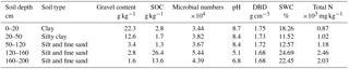
Note gravel content diameter ≥0.5 cm. SOC is soil organic content, DBD is dry bulk density, SWC is soil water content, and Total N is total nitrogen content.

2.2 Eddy covariance observations

We have continuously monitored CH₄, carbon dioxide (CO₂), water (H₂O), and heat flux using a standard EC system tower 3 m above the ground. CH₄ flux was measured with an open-path CH₄ analyzer system (Fig. 1d; LI-7700, Li-cor Inc., Lincoln, NE, USA). The precision is 5 ppb, with RMS noise at 10 Hz and 2000 ppb. The instrument was placed on site on 8 August 2011 and then connected to a three-dimensional sonic anemometer (heat and water flux; CSAT3, Campbell Scientific, and Logan, UT, USA; the precision is 0.1 ^∘C with an accuracy within 1 % of the reading for half-hour measurements) and an open-path infrared gas analyzer (CO₂ flux; LI-7500A, Li-cor Inc., Lincoln, NE, USA; the precision is 0.01 $\mathrm{\mu }\mathrm{mol}{\mathrm{m}}^{-\mathrm{2}}{\mathrm{s}}^{-\mathrm{1}}$ with an accuracy within 1 % of the reading for half-hour measurements; zero drift per degree Celsius is typically ±0.1 ppm) on 1 January 2012, when the system worked steadily. Monitoring data were recorded and stored at 10 Hz using a data logger (LI-7550, Li-cor Inc., Lincoln, NE, USA).

The operation, calibrations, and maintenance of the EC system followed standard procedures. To reduce the LI-7500A surface heating–cooling influence on CO₂ and H₂O molar densities in tough environments, each year “summer style”, in which the surface temperature setting was 5 ^∘C, was used in Li-7500A from 1 May to 30 September. “Winter style”, in which the surface temperature setting was −5 ^∘C, was used from 1 October to 30 April the next year in Li-7500A. Calibrations of CO₂, water vapor, and dew point generator measurements for LI-7500A analyzers were performed regularly by the China Land–Atmosphere Coordinated Observation System (CLAROS). Up-and-down mirrors of LI-COR 7700 were cleaned regularly every 30 days to make sure the signal strength was stronger than 80. All of these instruments were powered by solar panel and battery.

2.3 Micrometeorological and soil measurements

A wide range of meteorological variables were measured by a standard automatic meteorological tower 3 m above the ground and 5 m north of the EC tower. Net radiation (Rn) and albedo were measured with a four-component radiometer (Rn; CNR-1, Kipp and Zonen, the Netherlands). Air temperature (T_air), air relative humidity, and atmospheric pressure were measured with a temperature and humidity sensor (HMP45C, Vaisala Inc., Helsinki, Finland) in the meteorological tower. A rain gauge (TE525MM, Texas Electronics Inc., Dallas, TX, USA) was used to measure precipitation. Wind speed and direction were observed using a propeller anemometer placed on the top of the meteorological tower.

We also measured soil heat fluxes, soil temperature, and soil relative water content (SWC). In August 2010, we installed sensors for soil environment and surface energy exchange monitoring 10 m apart from the EC tower. Two self-calibrating soil heat flux (SHF) sensors (HFP01) were placed 5 and 15 cm below the ground. A group pF meter sensor (Geoprecision, Germany) was embedded in the soil under the meteorological tower to measure soil temperature (T_soil) at 0, 5, 10, 15, 20, 30, 40, 50, 70, 80, 100, 150, 160, and 200 cm of depth. The pF meter sensors also measured SWC at 10, 20, 40, 80, and 160 cm of depth.

All of the above environmental parameters were synchronously monitored with EC, and the data were recorded every 30 min by CR3000 (data logger, Campbell Scientific Ltd., Salt Lake City, UT, USA). The air temperature sensors, the humidity sensors, and the pF meter sensors were calibrated in the State Key Laboratory of Frozen Soil Engineering at the Chinese Academy of Sciences in order to ensure the measurement accuracy was within ±0.05 ^∘C and ±5 %.

We also sampled soil profiles for soil physical and chemical measurements with one $\mathrm{1}\mathrm{m}\times \mathrm{1}\mathrm{m}\times \mathrm{2}\mathrm{m}$ pit 10 m from the EC tower in August 2010. Five profile samples were taken from the pit at depths of 0–20, 20–50, 50–120, 120–160, and 160–200 cm. Sampling at each depth was repeated five times and the samples of the same depths were then well mixed. After that, the mixed soil sample of each depth was stored in aluminum boxes and carefully sealed to prevent gas exchanges with air. The clod method was used to investigate the field wet bulk density (weight of soil per unit volume; Cate and Nelson, 1971). The soil moisture content was calculated gravimetrically with the ratio of the mass of water present to the oven-dried (60 ^∘C for 24 h) weight of the soil sample. The soil organic carbon (SOC) content of the air-dried soil samples was analyzed using the wet combustion method, Walkley–Black modified acid dichromate digestion, FeSO₄ titration, and an automatic titrator. Total nitrogen (TN) and pH were measured using standard soil test procedures from the Chinese Ecosystem Research Network.

To understand the potential effect of soil thawing and freezing dynamics on CH₄ fluxes, we also reconstructed and verified semi-monthly data of soil ALT. Following Muller's original definition, ALT is the maximum thaw depth in the late autumn using a linear interpolation of T_soil profiles between two neighboring points above and below the 0 ^∘C isotherm (Muller, 1947). We used records of the soil thawing thickness measured with a self-made geological probe to verify the ALT data semi-monthly. More information about the measurement procedure was previously described by Wu and Zhang (2010a).

2.4 Microbial activity

To understand how soil microbial activity may have impacted the CH₄ fluxes, we sampled 100 g of soils for soil microbial activity measurements. These soils were obtained using a soil sample drill device (∅=0.03 m), with depths of 0–25 cm taken every 5 days within 100 m of the EC tower. The sampled soil was fully mixed and divided into two equal parts. Each part was then stored in sterilized aluminum boxes and then placed in liquid nitrogen before sending to the lab for microbe RNA extraction. We then used a real-time polymerase chain reaction (PCR) method to genetically test methanotrophic–archaeal methanogens, and the procedure was repeated three times for each sample. By setting the maximum methanotrophic–archaeal methanogen gene expression cyclic number as 1, we calculated the variety coefficient of methanotrophic and archaeal methanogen gene expressions (ΔI and ΔII, respectively; %) with Eq. (1):

$$\begin{array}{}\text{(1)}& {\displaystyle }{\mathrm{\Delta }}_i=x_i/X_{\mathrm{Max}}.\end{array}$$

Δ_i is for the ith methanotrophic–archaeal methanogen gene expression; x_i is the methanotrophic–archaeal methanogen gene expression cyclic number of the ith time; x_Max is the maximum methanotrophic–archaeal methanogen gene expression cyclic number of the soil group from 2012 to 2016.

2.5 EC data processing and data filtering

Data collected from 1 January 2012 to 31 December 2016 were used in this study. Before processing, we removed data that were recorded at the time of precipitation events or with a LI-7700 signal strength under 85. We first processed the raw data in EddyPro (version 6.2.0, Li-cor, Lincoln, NE, USA). We adopted standardized procedures recommended in Lee et al. (2006) to process half-hourly flux raw measurements to ensure their quality.

• 1.

  Data were processed through statistical analysis in EddyPro including spike removal (accepted spikes <5 % and replaced spikes with linear interpolation), amplitude resolution (range of variation: 7.0σ; number of bins: 100; accepted empty bins: 70 %), dropouts (percentile defining extreme bins: 10; accepted central dropouts: 10 %; accepted extreme dropouts: 6 %), absolute limits ($-\mathrm{30}\mathrm{m}{\mathrm{s}}^{-\mathrm{1}}<U<\mathrm{30}\mathrm{m}{\mathrm{s}}^{-\mathrm{1}}$, $-\mathrm{5}\mathrm{m}{\mathrm{s}}^{-\mathrm{1}}<W<\mathrm{5}\mathrm{m}{\mathrm{s}}^{-\mathrm{1}}$, $-\mathrm{40}{}^{\circ }\mathrm{C}<T_{\mathrm{soil}}<\mathrm{40}{}^{\circ }\mathrm{C}$; $\mathrm{200}\mathrm{\mu }\mathrm{mol}{\mathrm{mol}}^{-\mathrm{1}}<{\mathrm{CO}}_{\mathrm{2}}<\mathrm{500}\mathrm{\mu }\mathrm{mol}{\mathrm{mol}}^{-\mathrm{1}}$, $\mathrm{0}\mathrm{\mu }\mathrm{mol}{\mathrm{mol}}^{-\mathrm{1}}<{\mathrm{H}}_{\mathrm{2}}\mathrm{O}<\mathrm{40}\mathrm{\mu }\mathrm{mol}{\mathrm{mol}}^{-\mathrm{1}}$, $\mathrm{0.17}\mathrm{\mu }\mathrm{mol}<{\mathrm{CH}}_{\mathrm{4}}<\mathrm{1000}\mathrm{\mu }\mathrm{mol}$), skewness and kurtosis ($-\mathrm{2.0}<\text{skewness lower limit}<-\mathrm{1.0}$, $\mathrm{1.0}<\text{skewness upper limit}<\mathrm{2.0}$; $\mathrm{1.0}<\text{kurtosis lower limit}<\mathrm{2.0}$, $\mathrm{5.0}<\text{kurtosis upper limit}<\mathrm{8.0}$), discontinuities (hard-flag threshold: U=4.0, W=2.0, T_soil=4.0, CO₂ =40, CH₄ =40, and H₂O =3.26; soft-flag threshold: U=2.7, W=1.3, T_soil=2.7, CO₂ =27, CH₄ =30, and H₂O =2.2), angle of attack (minimum angle of attack $=-\mathrm{30}$; maximum angle attack =30; accepted number of outliers =10 %), and steadiness of horizontal wind (accepted wind relative instationarity =0.5) (Vickers and Mahrt, 1997; Mauder et al., 2013).

• 2.

  The data were then corrected using atmosphere physical calculations expressed by axis rotations of tilt correction (double rotation), time lags compensation (covariance maximization), and compensating density fluctuations of Webb–Pearman–Leuning (Webb et al., 1980). When CO₂ and H₂O molar densities are measured with the Li-cor 7500/Li-cor 7500A in cold environments (low temperatures below −10 ^∘C), a correction should be applied to account for the additional instrument-related sensible heat flux due to instrument surface heating–cooling. Thus, we implemented the correction according to Burba et al. (2008), which involves calculating a corrected sensible heat flux (H^′) by adding estimated sensible heat fluxes from key instrument surface elements, including the bottom window (H_bot), top window (H_top), and spar (H_spar), to the ambient sensible heat flux (H):

  $$\begin{array}{}\text{(2)}& {\displaystyle }{H}^{\prime }=H+H_{\mathrm{bot}}+H_{\mathrm{top}}+\mathrm{0.15}\cdot H_{\mathrm{spar}}.\end{array}$$
• 3.

  Quality assurance (QA) and quality control (QC) were ensured through spectral analysis and correction analysis in EddyPro. Spectra and co-spectra calculations used power-of-two samples to speed up the fast Fourier transform (FFT) algorithm. Here we checked the “Filter (co-)spectra according to Vickers and Mahrt (1997) test results” box in EddyPro, which would then disregard EC flux time series that would likely create artifacts in spectral and co-spectral shapes. We also used the Foken and Wichura (1996) and Mauder et al. (2013) micrometeorological quality tests embedded in EddyPro to filter low-quality EC time series data. Low-frequency-range spectral correction was performed considering high-pass filtering effects. High-frequency-range spectral correction was carried out considering low-pass filtering effects (Moncrieff et al., 2004).

• 4.

  We chose values of “0”, “1”, and “2” to flag the processed flux data into three quality classes in EddyPro. The combined flag attains the value 0 for the best-quality fluxes, 1 for fluxes suitable for general analysis, such as annual budgets, and 2 for fluxes that should be discarded from the dataset of results. For our dataset, approximately 67 % of the data fell into Class 0, 12 % in Class 1, and 21 % in Class 2.

• 5.

  Our analysis indicated that, under average meteorological conditions, 80 % of the flux (footprint) came from an area within 175 m of the EC tower.

In addition, we also adopted the method in Burba et al. (2008) to adjust the half-hour flux data to avoid apparent measurement errors. In doing this, we rejected half-hour flux data that fell into one of the following situations: (1) incomplete half-hour measurements, (2) measurements under rain impacts, (3) nighttime measurements under stable atmospheric conditions (friction velocity $U^{*}<\mathrm{0.1}$ m s⁻¹), and (4) abnormal values detected by a three-dimensional ultrasonic anemometer. This screening resulted in the rejection of about 20.7 % of all the flux data.

After the above data QC, there was a 28.7 % data gap for CH₄ fluxes over the entire period. These data gaps were then filled according to the method described in the literature (Falge et al., 2001; Papale et al., 2006). We used a linear interpolation to fill the gaps if they were less than 2 h, a method described in Falge et al. (2001) to fill gaps greater than 2 h but less than 1 day, and an artificial neural network approach as described in Papale et al. (2006) and Dengel et al. (2013) to fill gaps greater than 1 day.

The quality of the dataset was evaluated using the equation of energy closure:

$$\begin{array}{}\text{(3)}& {\displaystyle }\text{EBR}=\sum \left(H+\mathit{\lambda }E\right)/\sum \left(R_{\mathrm{n}}-G-S\right),\end{array}$$

where the EBR is surface energy balance ratio, H is heat flux, λE is latent heat, R_n is net radiation, G is SHF, and S is heat storage of the vegetation canopy. As vegetation coverage at this research site is sparse, S is ignored. From 2012 to 2016, the average EBR value at the Beilu'he EC site was about 0.675, falling within the range of 0.34 to 1.69 in an analysis of energy balance closure for global FLUXNET sites (Wilson et al., 2002).

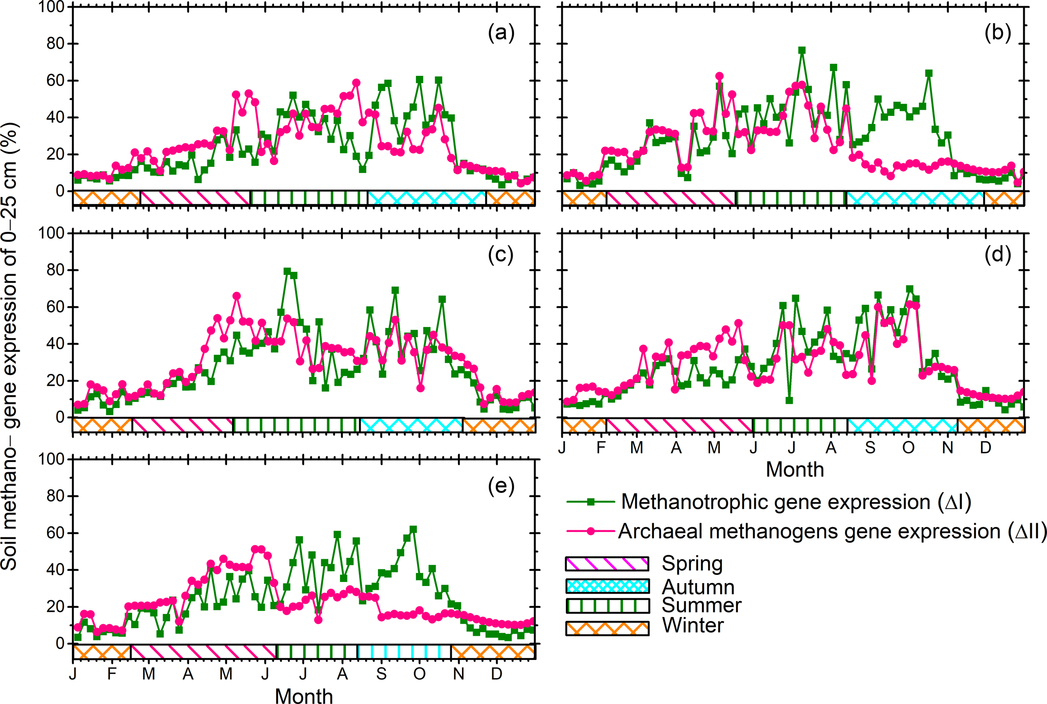
Figure 2 Annual patterns of soil methanogen gene expression of 0–25 cm soil depth for the years (a) 2012, (b) 2013, (c) 2014, (d) 2015, and (e) 2016.

We analyzed two different major sources of CH₄ flux gap-filling uncertainty. The first kind of uncertainty came from the U^* threshold estimate. Following Burba et al. (2008), we excluded the probably false low CH₄ flux at low U^*. However, it was difficult to determine the value for the U^* threshold. For instance, when choosing a lower U^* threshold, the associated lower flux would contribute to the gap filling and the annual gross (Loescher, et al., 2006). Here we used the variance from 5 % to 95 % of the bootstrapped values to provide an estimate on the uncertainties caused by different U^* thresholds. The second uncertainty source was due to insufficient power supply. In this research, all instrument power was supplied by solar panels. Extended periods of rainy, cloudy, and snowy weather would cause the instrument to stop working due to an insufficient power supply. When we used the gap-filling method mentioned above, it would cause the CH₄ flux to deviate from the true value. To our knowledge, the CH₄ flux data were largely uncertain under rainy conditions.

2.6 New classification system of the four seasons based on microbial activity classification

We redefined the four seasons of spring, summer, autumn, and winter based on the microbial activity parameters of the new seasons (Fig. 2), ALT variability coefficients (ALT variability coefficient = (ALT${}_{i+\mathrm{1}}-$ ALT_i)/ALT_Max, where ALT_Max is the maximum of ALT per year), and T_soil. Below, we describe the start date of each season (the end date of a season is the day immediately before the start of the next season).

Spring starts at the first day of two consecutive observation periods fulfilling both (1) (ΔII +ΔI)/2≥15 % and (2) the ALT variability coefficient ≥0.05.

Summer starts on the first day of two consecutive observation periods when (1) (ΔII +ΔI)/2≥45 %, (2) the ALT variability coefficient is ≥0.35, and (3) 5 successive days have a T_soil at 40 cm of soil depth ≥0 ^∘C.

Autumn starts on the first day of two consecutive observation periods when (1) (ΔII +ΔI)/2≥55 %, (2) the ALT variability coefficient is ≥0.60, and (3) 5 successive days have a T_soil of 10 cm<5 ^∘C.

Winter starts on the first day of two consecutive observation periods that have (1) (ΔII +ΔI)/2<15 % and (2) the ALT variability coefficient <0.05.

To test the robustness of our new seasonal division method in our methane cycle analysis, we compared empirical CH₄ flux estimates using different season definitions (Table 2). In addition to our new method that was based on top soil microbe activity, T_soil of 0–40 cm, and permafrost active layer variability (hereafter referred to as SMT), we also used three conventional methods, based on (i) vegetation cover and temperature change (VCT), (ii) Julian months (JMC), and (iii) vegetation phenology change (VPC). The VCT method splits a year into a plant growing season and a nongrowing season; the JMC method assumes May to October as a plant growing season, and November to the following April as a nongrowing season; and the VPC method defines a plant growing season as the period between the time when all dominant grass species (Carex moorcroftii Falc. ex Boott, Kobresia tibetica Maxim, Androsace tanggulashanensis, Rhodiola tibetica) germinate and when they all senesce.

Table 2 Measurements of four seasons from 2012 to 2016.

^a Based on vegetation cover and temperature change (VCT) (Lund et al., 2010; Tang et al., 2013; Song et al., 2015). ^b Based on Julian months (JMC) (Wei et al., 2015a). ^c Based on vegetation phenology change (VPC). Spring, summer, autumn, and winter are based on parameters of microbial activities, ALT variety coefficient, and T_soil (SMT).

2.7 Statistical analyses

To understand the connections between CH₄ fluxes and associated environmental factors, we performed a series of statistical analyses, including correlation, principal component analysis (PCA), and linear regression analyses, in IBM SPSS (IBM SPSS Statistics 24; IBM, Armonk, NY, USA). Specifically, we used bivariate correlation to examine pairwise relationships between environmental factors and CH₄ fluxes. We also used PCA and linear regressions to explore the sensitivity of CH₄ fluxes to simultaneous environmental fluctuations in wind speed, T_air, air relative humidity, Rn, vapor pressure deficit (VPD), albedo, SHF, SWC, and T_soil. Before performing PCA and linear regressions, the entire dataset was examined for outliers (Cook's distance, <0.002), homogeneity of variance (Levene's test, p<0.05), normality (Kolmogorov–Smirnov test; smooth line for histogram of Studentized residuals), collinearity (variance inflation factor, $\mathrm{0}<\text{VIF}<\mathrm{10}$), potential interactions (t test, p<0.05), and independence of observations (t test, p<0.05).

We performed structural equation modeling (SEM) to evaluate the effects of environmental variables on CH₄ fluxes for different seasons. SEM is a widely used multivariate statistical tool that incorporates factor analysis, path analysis, and maximum likelihood analysis. This method uses a priori knowledge of the relationships among focus variables to verify the validity of hypotheses. Here we performed SEM analyses with AMOS 21.0 (Amos Development Corporation, Chicago, IL, USA). All data are presented as mean values with standard deviations.

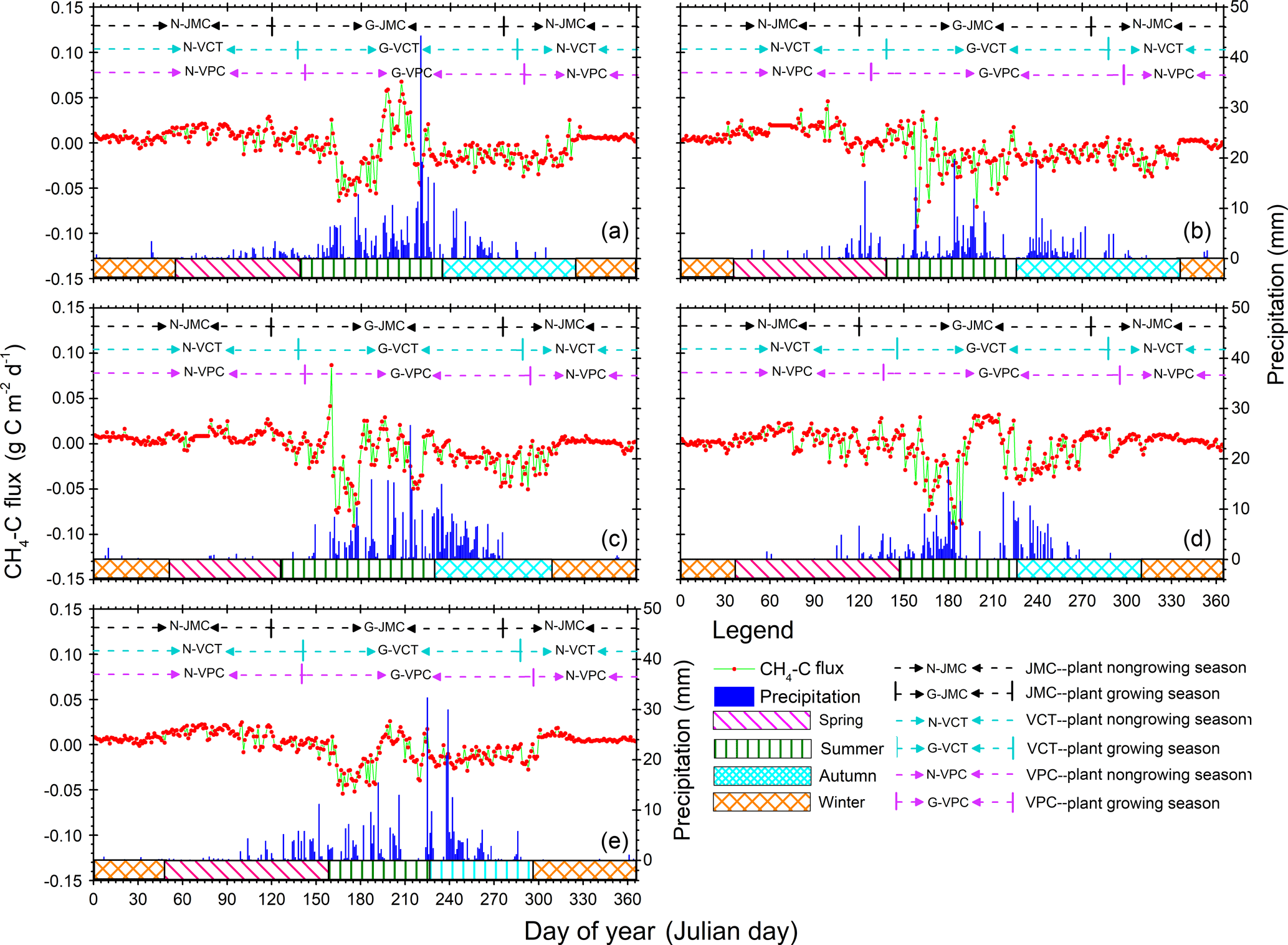
Figure 3 Annual patterns of diel methane (CH₄) flux and precipitation variations from 2012 to 2016. Positive values indicate CH₄ release and negative values indicate CH₄ uptake by ecosystems. Red dots and light green lines are CH₄-C flux variation, and the deep blue histograms show diel precipitation accumulation. Pink, olive, cyan, and orange blocks mean spring, summer, autumn, and winter seasons, respectively, according to our new method of SMT (see Sect. 2). Black, cyan, and pink dotted lines with bars separated the plant growing from nongrowing seasons and stand for seasons with the JMC, VCT, and VPC methods, respectively. Details about the JMC, VCT, and VPC methods can be found in Sect. 3.2.

3 Results

3.1 Meteorological conditions

We first reported the statistics of the meteorological conditions at the Beilu'he permafrost weather station between 2012 and 2016. Mean annual T_air was −4.5^∘ (Fig. S1 in the Supplement), with minimum and maximum mean diel temperatures of −21.6^∘ (12 January 2012) and 13.8^∘ (28 July 2015), respectively. Average net radiation was 82.8 W m⁻², with the maximum in August (136.2 W m⁻²; Fig. S2). The average VPD was about 0.3, with maximum and minimum values of 0.98, and 0.02, respectively (Fig. S3). Mean annual precipitation was 335.4 mm (Fig. 3), which was primarily based on rain and snowfall (only occupied 7 %). Maximum and minimum precipitation was recorded in 2013 (488.3 mm) and 2015 (310.0 mm), respectively. The majority of precipitation, approximately 92 %, hereby occurred in the summer. During the winter, precipitation was rare, with mean values around 6.7 mm. Spring was another important rainfall period in addition to summer, with mean precipitation being about 37.5 mm, or 8∼17 % of the total.

The Beilu'he site is windy during most of the year (Fig. S4). Its annual average speed was 4.4 m s⁻¹ from 2012 to 2016, while the principal direction of the strongest winds was from the southwest. Late autumn, winter, and early spring drought brought increased risks of dust-blowing days, with an average of 122 days within a year. Its summer average wind speed was about 3.30 m s⁻¹, predominantly driven by the southwest wind.

The SWC and T_soil variability from 2012 to 2016 at the field site are summarized in Figs. S5 and S6, respectively. Mean SWC of depths of 10, 20, 40, 80, and 160 cm were 14 %, 9 %, 8 %, 14 %, and 19 %. T_soil of depths <100 cm corresponded with the T_air changes, but showed stronger differences at depths >100 cm. The T_soil at 200 cm of depth showed a remarkable difference from that of other layers. The reason could be the occurrence of peat in this layer, and that, during winter, the peat layer was not completely frozen. Figure S7 shows SHF half-hour and diel-scale variability of 5 and 15 cm in depth. The annual mean value of SHF at 5 and 15 cm of depth is 7.6 and 6.8 W m⁻², respectively.

Finally, Fig. S8 shows the site's average soil freezing and thawing dynamics observed from January 2012 to December 2016. The average ALT is 4.4 m from 2012 to 2016. At 40 cm of depth the duration of the active layer ranged from 174 to 188 days, with an average variation of up to 14 days.

3.2 Annual, seasonal, and diel variabilities in methane fluxes

Our results indicated that the Beilu'he site was a CH₄ sink, with an annual mean strength of $-\mathrm{0.86}\pm \mathrm{0.23}$ g CH₄-C m⁻² (95 % confidence interval; negative values mean CH₄ sinks; positive values mean CH₄ sources). The strength of the CH₄ sink varies across different years from $-\mathrm{0.57}\pm \mathrm{0.27}$ g CH₄-C m⁻² yr⁻¹ in 2015 to $-\mathrm{1.49}\pm \mathrm{0.38}$ g CH₄-C m⁻² yr⁻¹ in 2014 (Fig. 3). The amount of gene expression by methanogens and methanotrophs at 0–25 cm soils in March and November, for instance, was about 16.8 % and 35.6 %, respectively, suggesting strong microbial activities even during the cold and dry plant nongrowing season (Fig. 2).

We also clearly observed CH₄ seasonal variations (Fig. S9) in both the number of CH₄ exchanges and their diel cycles (Fig. 4). Across different seasons the footprint of the monitored CH₄ flux changed following the change of the prevalent wind direction. In winter and spring, the major footprint was from east of the EC tower; while in summer and autumn, the major footprint was from west and north of the EC tower (Fig. S4).

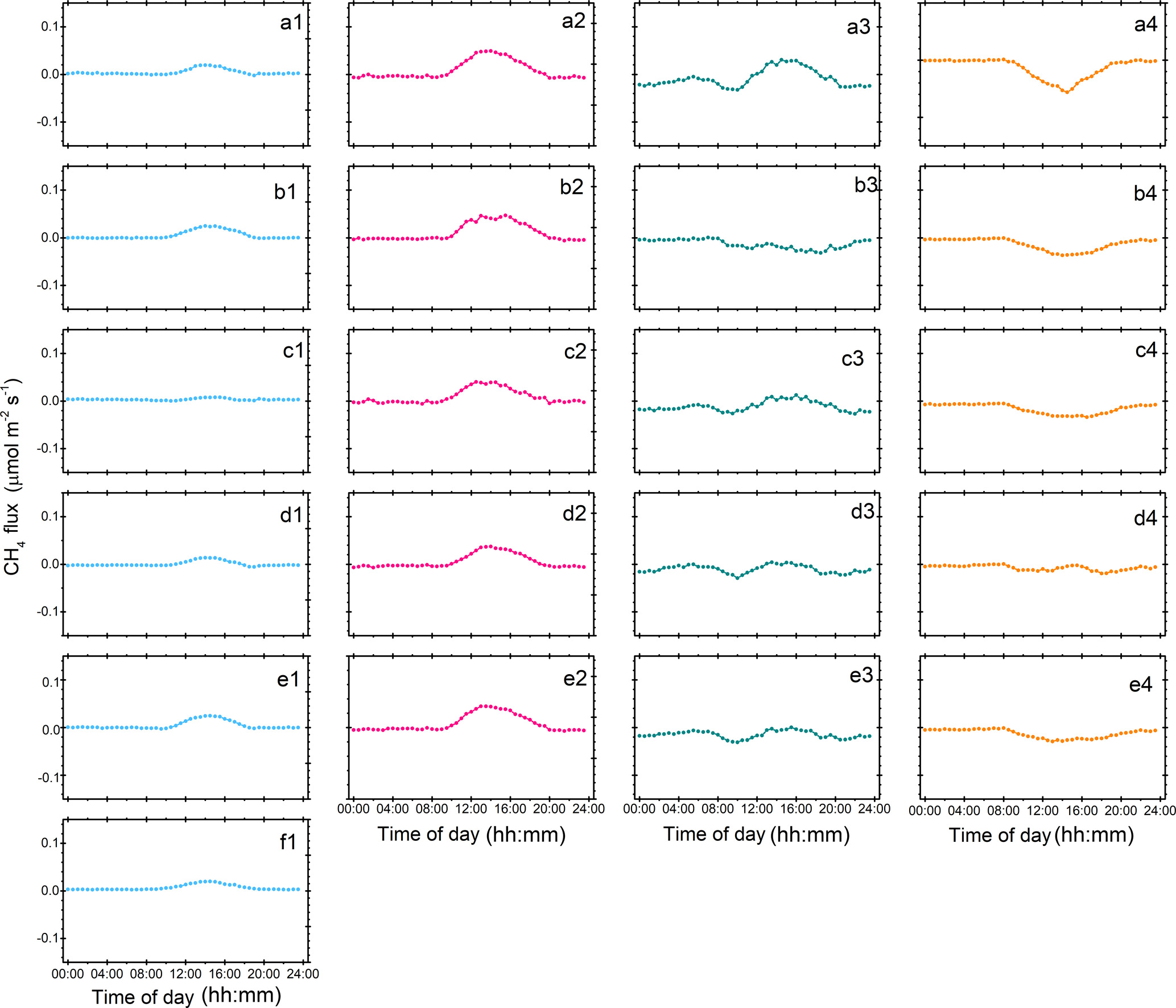
Figure 4 Diel CH₄ fluxes from 2012 to 2016 for different seasons. Blue, pink, green and orange, represent winter, spring, summer, and autumn, respectively: (a1–a4) 2012, (b1–b4) 2013, (c1–c4) 2014, (d1–d4) 2015, (e1–e4), and (f1) 2016.

In winter, the net CH₄ flux at the Beilu'he site was an atmospheric source, with an average annual rate of 0.41±0.16 g CH₄-C m⁻² yr⁻¹ or 4.35±0.33 mg CH₄-C m⁻² d⁻¹ (Fig. S9a). It should also be noted that since the investigation started on 1 January 2012 and ended on 31 December 2016, the 2011–2012 and 2016–2017 winters were only about half of the regular length. The diel CH₄ cycle of an average winter day was characterized by one single emission peak around 10:30–17:30 Beijing time (note all times hereafter are in Beijing time; Fig. 4a1–f1).

In spring, the Beilu'he site was a CH₄ source of 0.90±0.37 g CH₄-C m⁻² yr⁻¹ (Fig. S9b), accounting for 53 % of annual CH₄ emissions, or 1.81±0.22 mg CH₄-C m⁻² d⁻¹. For a typical spring day (Fig. 4a2–e2), diel CH₄ emission usually started at around 10:00–10:30, when the thin ice layer on the soil surface started to thaw. It then reached the peak at 12:30–13:30. The emission peak started to weaken at around 15:30–16:00 and reached around zero or even turned into a small sink after 20:00.

Table 3 Correlation coefficients between CH₄ fluxes and environment factors on half-hour timescales.

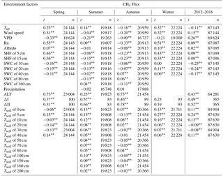
Note ${}^{**}$ means p<0.01; ^* means p<0.05; r values are for the relationship between CH₄ flux and environment factors. T_air means air temperature of 3 m above the ground surface. VPD is vapor pressure deficit, Rn is net radiation, and SWC is soil water content. ALT is active layer thickness, which fitted through the depth of soil 0^∘ in Surfer 8.0, and the data are removed as meaningless in winter. T_soil is the temperature of the soil. In spring and winter, precipitation data are too sparse for statistical analysis. ΔI is the soil 0–25 cm archaeal methanogen gene expression, and ΔII is the soil 0–25 cm methanotrophic gene expression. The coefficients (r) between CH₄ flux and ΔI and ΔII are obtained using the synchronous CH₄ fluxes averaged for 5 days.

In summer, the Beilu'he site was a CH₄ sink of $-\mathrm{0.99}\pm \mathrm{0.18}$ g CH₄-C m⁻² yr⁻¹ (Fig. S9c), or $-\mathrm{13.28}\pm \mathrm{0.38}$ mg CH₄-C m⁻² d⁻¹. The diel cycle of CH₄ fluxes in summer was characterized by two absorption peaks and one small emission peak (Fig. 4a3–e3). With T_air increasing after sunrise, the soil started to absorb atmospheric CH₄ and this soil uptake process reached its first peak at around 09:30–10:30. After that, the continuously increasing T_air turned to suppress CH₄ uptake and promote CH₄ emissions, likely due to different temperature sensitivities of methanotrophic and methanogenic bacteria. At around 15:30–16:00, when T_air reached the maximum (Fig. S1b), CH₄ emission also reached its peak. The following temperature decrease in the late afternoon again reversed the CH₄ uptake–emission process, and by sunset we observed another CH₄ sink peak. The rate of CH₄ sink then decreased again through the night with further decreasing temperature.

Autumn was another season with a net CH₄ sink, with the season having the highest observed value for the site as a CH₄ sink in 2013 (Fig. S9d). The CH₄ sink in autumn varied between $-\mathrm{0.69}\pm \mathrm{0.19}$ g CH₄-C m⁻² (2015) and $-\mathrm{1.59}\pm \mathrm{0.33}$ g CH₄-C m⁻² (2013), with an average diel rate of $-\mathrm{1.19}\pm \mathrm{0.48}$ g CH₄-C m⁻² yr⁻¹ or $-\mathrm{13.31}\pm \mathrm{0.28}$ mg CH₄-C m⁻² d⁻¹. The diel dynamics of autumn CH₄ fluxes was like a letter “V”, with a single sink peak during 13:30–15:30 (Fig. 4a4–e4).

3.3 Response of methane fluxes to changes in environmental factors

Diel fluxes of CH₄ were correlated either positively or negatively with many biotic and abiotic environmental factors (Table 3). Positive factors include metagenomics of both methanotrophic (r=0.52, p<0.01) and methanogens (r=0.49, p<0.01) at 0–25 cm soils, ALT (r=0.43, p<0.01), and wind speed (r=0.15, p<0.01). Important negative factors include VPD ($r=-\mathrm{0.26}$, p<0.01), SWC at all depths (varied r values between −0.17 and −0.26, p<0.01), T_air ($r=-\mathrm{0.11}$, p<0.01), and air pressure ($r=-\mathrm{0.15}$, p<0.01). The correlation signal between CH₄ fluxes and T_soil changed with soil depths (varied r values between −0.09 and 0.24, p<0.01). Furthermore, path analysis results showed that T_soil values at 5 and 10 cm were the most important factors, which together contributed about 25 % of the relative importance coefficient. Following these factors in importance were SWC at 80 cm (14 %) and 20 cm (12 %) and T_soil at 20 cm (8 %).

Further analyses suggested that dominant control factors of CH₄ fluxes also changed among different seasons. In spring, Rn was the most important factor, with a relative importance coefficient near 60 %, followed by SHF at 5 cm (9 %) and SWC at 20 cm (6 %). Table 4 shows the results of the PCA. In spring, PC1 explained 63 % of the CH₄ variations, which was positively correlated with T_air, VPD, Rn, SHF of 15 cm, ALT, ΔI, SWC of 10–40 cm, T_soil of 0 cm, T_soil of 5–20 cm, and T_soil of 30–50 cm and negatively correlated with wind speed. The PC2 explained about 23 % of CH₄ flux variations. The first four principal components explained about 86 % of the CH₄ variations.

In summer, CH₄ fluxes were mostly related with T_soil at 100 and 200 cm, with a relative importance coefficient of about 30.2 % and 26.5 %, respectively. Other important environmental determinants of CH₄ fluxes were T_soil at 70 cm (12.3 %) and T_soil at 0–20 cm (11.4 %). The first four principal components explained about 88 % of the CH₄ variations (Table 4). PC1 explained 70 % of the CH₄ variations and was positively correlated with wind speed, T_air, VPD, SHF of 15 cm, ALT, ΔI, SWC of 50–160 cm, precipitation, T_soil of 0 cm, T_soil of 5–40 cm, T_soil of 50–80 cm, and T_soil of 100–200 cm, but negatively correlated with Rn and SWC of 10–40 cm.

In autumn, Rn and T_soil at 5–20 cm had the highest relative importance coefficients for explaining the CH₄ flux variation. The first four principal components explained about 86 % of the CH₄ variations (Table 4). PC1 explained 69 % of the CH₄ variations and was positively correlated with T_air, VPD, Rn, SHF of 15 cm, ALT, ΔI, SWC of 10–40 cm, SWC of 50–160 cm, T_soil of 0 cm, T_soil of 5–40 cm, T_soil of 50–80 cm, and T_soil of 100–200 cm, but negatively correlated with wind speed.

Table 4 Principal component analysis (PCA) of the environmental factors.

Note PC means principal component. Before PCA, SWC was divided into three parts, 10–20, 10–40, and 50–160 cm, according to a collinearity test in four seasons. T_soil was divided into six parts of T_soil of 0 cm, T_soil of 5–20 cm, T_soil of 5–40 cm, T_soil of 30–50 cm, T_soil of 50–80 cm, and T_soil of 60–200 cm according to a collinearity test in different seasons.

During winter, Rn was again the most important factor (34 % relative importance coefficient), followed by T_soil at 0–40 cm (27 % in total) and a SHF of 15 cm (17 % in total), in determining CH₄ fluxes. The first four principal components explained about 96 % of the CH₄ variations (Table 4). PC1 explained 75 % of the CH₄ variations and was positively correlated with wind speed, T_air, VPD, Rn, SHF of 15 cm, ΔI, T_soil of 0 cm, and T_soil of 5–20 cm.

3.4 Empirical model comparison for different CH₄ flux season classification system

Lastly, we also compared how different season definitions, including the methods of SMT, VCT, JMC, and VPC, may have impacted the predictability of CH₄ fluxes. We established empirical maximum likelihood models between all environmental factors and diel CH₄ fluxes over each season, and then we compared modeled CH₄ fluxes and field observations under those methods of different seasonal definitions (Fig. 5). We found that the agreement between modeled and observed CH₄ fluxes, using the new SMT method, reached R²=0.28, almost twice that of the VPC (R²=0.17) and VCT (R²=0.14) methods, and more than three times that of the JMC method (R²=0.08; Fig. 5). Hence, the comparison suggested that our new method could better model CH₄ fluxes over a year. The use of the traditional plant growing season versus nongrowing season definitions may also underestimate or overestimate CH₄ sinks or sources, especially when many studies assume CH₄ is close to zero during the plant nongrowing season. Furthermore, the new SMT method accurately captures the impact of spring and autumn permafrost thawing–freezing cycles on CH₄ fluxes and the different preferable environments for methanogens and methanotrophic bacteria during the summer season, while conventional methods do not.

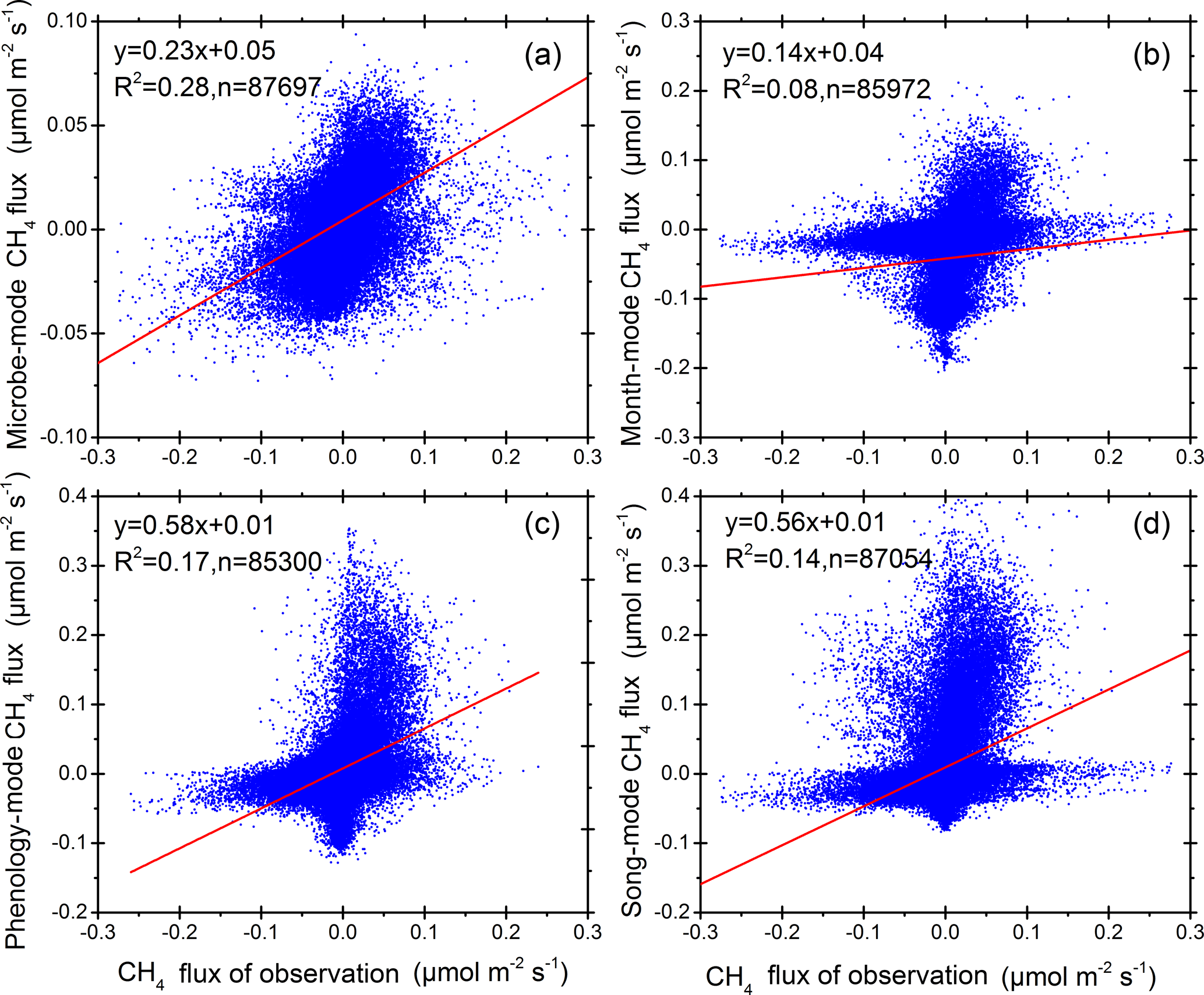
Figure 5 Regression comparison between observation and modeled methane fluxes with four different seasonal definitions and classification models. Panels (a), (b), (c), and (d) are for the SMT, JMC, VCT, and VPC methods, respectively.

4 Discussion

4.1 Annual and season mean and diel variability

Our results suggested that the alpine steppe ecosystem in Beilu'he was a CH₄ sink of about $-\mathrm{0.86}\pm \mathrm{0.23}$ g CH₄-C m⁻² yr⁻¹ during the study period of 2012–2016. This sink strength is larger than that of previous reports from other sites of the QTP (Cao et al., 2008; Wei et al., 2012; Li et al., 2012; Song et al., 2015; Chang and Shi, 2015) and many other high-latitude Arctic tundra ecosystems, like northeast Greenland (Jørgensen et al., 2015), western Siberia (Liebner et al., 2011), and Alaska (Whalen et al., 1992; Zhuang et al., 2004; Whalen, 2005). Different soil hydrothermal conditions, which previous studies have shown will greatly influence CH₄ cycles in permafrost regions (Spahni et al., 2011; Kirschke et al., 2013), may partly explain the site difference in CH₄ dynamics. For example, compared to the wet and often snow-covered high-latitude Arctic tundra ecosystems, there is no or little snow cover during the cold season in the QTP alpine steppes (Table S1 in the Supplement). During winter, the Beilu'he meteorological data show that the snow cover lasting <33.7 h, with a SWC of 0–40 cm within a footprint <7.6 % from 2012 to 2016 (Table S1), is far below high-latitude Arctic tundra ecosystems. Jansson and Taş (2014) pointed out that relatively dry soils could facilitate the oxidation of CH₄ since the increased number of gaps between soil particles in dry soils enhances the diffusion of oxygen (O₂) and CH₄ molecules and promotes aerobic respiration of soil microorganisms (Wang et al., 2014; Song et al., 2015). Meanwhile, unfrozen or capillary water found in cold season permafrost soils ensures sufficient soil moisture for microbial activities, even in relatively drier and cold soils (Panikov and Dedysh, 2000; Rivkina et al., 2004). In addition, many previous studies used static chambers in CH₄ measurements and may not have included a plant nongrowing season (Wei et al., 2015a; Wang et al., 2014). Static chambers could underestimate CH₄ uptake because of the additional chamber heating-induced CH₄ emissions and frequent measurement gaps from overheating preventive shutdowns (Sturtevant et al., 2012).

We argued that seasonal freezing and thawing dynamics may be a key reason to explain the site's seasonal difference in CH₄ dynamics. Freezing and thawing processes are typical characteristics of the QTP permafrost (Wang et al., 2008, 2000; Qin et al., 2016). Our work suggests that freezing and thawing dynamics have played a critical role in governing permafrost seasonal and diel CH₄ cycling. For instance, while both spring and autumn are active seasons for the freeze–thaw dynamics of top soil layers and share many similarities, they have opposite CH₄ processes and soils that emit CH₄ during spring (Fig. S9b) but consume CH₄ during autumn (Fig. S9d). We hypothesize that the difference in the freezing and thawing processes of the two seasons may have played a critical role in determining the direction of CH₄ dynamics. In spring, the SWC of 10 cm, of 20–40 cm, of 80 cm, and of 160 cm depth is 12.4 %, 9.2 %, 11.4 %, and 13.6 %, respectively (Table S1). The active soil layer thaws from top to bottom (Jin et al., 2000; Cao et al., 2017), and the permafrost table is very shallow (about 10–45 cm) and often waterproof (Wu and Zhang, 2008; Song et al., 2015; Lin et al., 2015). The water thawed during the daytime would freeze again at night on the soil surface (Fig. S10a; Shi et al., 2006; Wu and Zhang, 2010b). The thin-ice layer could stop atmospheric gases of CH₄ and O₂ from getting into the soils (Gažovič et al., 2010). During autumn, the SWC is 15.3 % at 10 cm below ground, decreases to 9.4 % at 20–40 cm, and then increases to 13.6 % and 21.0 % at 80 cm and 160 cm, respectively (Table S1). However, soils are bidirectionally frozen from both the top (ground surface) and bottom (permafrost table), which is about 200–400 cm below ground (Fig. S8; Wu and Zhang, 2010a). On the one hand, the frozen soil of the ground surface (about 0–40 cm) prevents the outside liquid water from permeating. On the other hand, the freezing itself will reduce the liquid water content in the soil. Therefore, it creates finely closed anaerobic gaps that allow CH₄ and O₂ gases into deep soils (about 50–400 cm; Mastepanov et al., 2008, 2013; Zona et al., 2016). Meanwhile, the temperature of deep soils (about 50–400 cm) still remains at a relatively high level (Fig. S10b), and methanotrophic bacteria will still be active at this high T_soil (Fig. 2). This could be one important mechanism for autumn soil CH₄ consumption. In addition, in principal it is also possible that the observed seasonal variation in CH₄ flux may actually arise from the spatial variation in the footprint covered by the EC site (within 175  m), given that prevalent wind direction changes seasonally (Fig. S4). Nonetheless, we found that the same vegetation species and soil exist in different directions from the tower within the footprint (Fig. S11). This spatial vegetation and soil homogeneity rules out the potential influence of footprint changes on the sign of CH₄ balances and further confirms that seasonal soil freezing and thawing differences may likely be the main explanation for seasonal CH₄ variations.

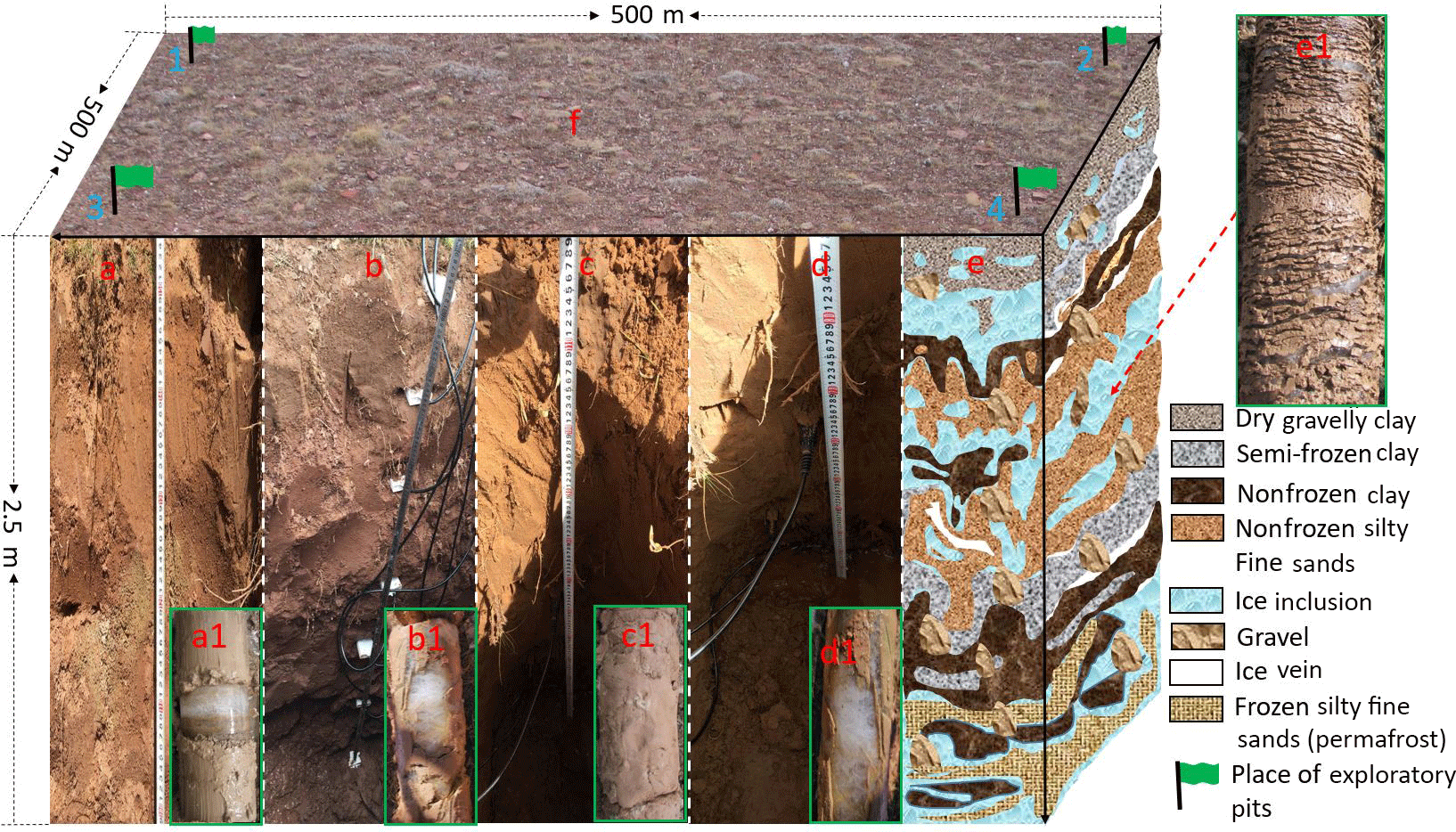
Figure 6 Location of exploratory pits and drillings in this study in autumn: (f) photo of a typical ground surface (16 October 2014). Green flags represent the location for the soil survey using test pits and drilling. (a, b, c, d) Soil profiles of 0–250 cm of depth at the north (1), south (2), east (3), and west (4) corners of the eddy covariance footprint, respectively. (a1, b1, c1, d1) Drilling cores, with clear ice (white) in (a1, b1, d1), but not in (c1). (e) An illustration that combines results from drillings, test pits, and multichannel ground-penetrating radar (Malå Geoscience, Sweden) for active layer variations in permafrost area during the autumn season. (e1) A core sample of the same drilling (16 October 2014).

Furthermore, we suggested that the specific autumn soil vertical structure may help to explain why the site was a CH₄ sink, unlike the CH₄ source in spring. The sequential probing data enables us to establish a rough estimate on the soil vertical structure during the autumn thawing–freezing process, in which the vertical distribution of clay, sandy soils, and soil organic layers was mixed like a multilayer structure, rather than forming a gradual change (Fig. 6e). As the soil profile is vertically different in features such as soil density, thermal conductivity, latent heat, and soil salinity, we boldly conjecture that the T_soil, SWC, and soil microbial activities also had a similar layer type of vertical distribution. As a result, layers of frozen and thawed soils were not changing gradually but appeared like a layered structure too. This soil vertical structure trapped high concentrations of soil water between the frozen layers and was therefore highly anaerobic and suitable for CH₄ production. It may also allow speculation that biogenic CH₄ between frozen layers could not escape in autumn. The biogenic CH₄ would be trapped until the active soil layer was completely frozen in late autumn, and in some warmer years until early winter, and created frost cracks. This would enable it to escape and may explain why there was a large burst of CH₄ emissions in late autumn and early winter and may also explain the constantly weak CH₄ emission through the winter season, although methanogenic bacteria may have stopped functioning in the low temperatures of winter. Of course, further studies and direct data collection in the field will be needed to fully test the hypothesis.

4.2 Impacts of environmental, permafrost, and microbial activities on CH₄ fluxes

Our results demonstrated the important roles of climate, freezing and thawing dynamics, and soil microbe activities in regulating the direction and amount of CH₄ exchange between the atmosphere and ecosystems in permafrost areas. The key role of the above factors and processes was also confirmed by the better representation of seasonal CH₄ cycles by our new seasonal division method based on soil microbes, temperature, and permafrost dynamics rather than T_air or vegetation phenology. Here, we further discuss potential mechanisms of how environmental (including air and soil heat and water), freezing and thawing processes, and soil microbes control the production and absorption of CH₄.

First, it is noteworthy that both the strength and direction of correlations among CH₄ fluxes, SWC, and T_soil parameters changed with soil depths, particularly during spring and autumn, when active layer soils shifted between thawing and freezing regularly. The positive and negative CH₄ flux correlations with T_soil and SWC may suggest that the impacts of T_soil and SWC on CH₄ fluxes shall be treated as a holistic process (Table 3), rather than as separate ones. For instance, in autumn, the significant correlation between CH₄ fluxes and T_soil or SWC was positive at some soil depths, but negative at some other depths, reaching the maximum at the depth of 80 cm. Further, in situ observations suggested that soil organic matter and soil microbe number were also at a very high level at this depth, highlighting that the regulation of soil abiotic factors on CH₄ cycling may be highly influenced by soil biotic activities. In addition, the holistic soil heat–water process could also determine the concentration of soil inorganic ions, particularly during spring and autumn, which were critical factors controlling the amount of soil unfrozen water. Earlier studies suggested that soil unfrozen water is important for maintaining soil microbial activities in winter (Panikov and Dedysh, 2000; Rivkina et al., 2004). In the future we will include data for soil unfrozen water to test its role in regulating CH₄ exchanges in permafrost regions.

T_air and precipitation impact CH₄ fluxes indirectly through their influences on T_soil and SWC (Zhuang et al., 2004; Lecher et al., 2015). Such indirect influences may often be characterized with time-lagged effects (Koven et al., 2011). For instance, post-drought rainfall events in summer can first promote soil CH₄ consumption (summer of 2014). This is because certain soil moisture is needed for methanogenic bacteria to function (Del et al., 2000; Luo et al., 2012). Yet, prolonged rainfall will eventually cause CH₄ fluxes to change from negative (soils consume CH₄) to positive (soils emit CH₄) fluxes (for example, day 168 to 183 of 2015; Fig. 3d). After rainfall events, CH₄ flux gradually turned negative again with the decrease in SWC. As a result of these time-lagged effects, the correlation coefficient between CH₄ fluxes and precipitation often appears very low, although still statistically significant.

Second, soil methanogenic and methanotrophic bacteria could coexist with different optimal niches (e.g., ranges of T_air/T_soil and SWC; Zhuang et al., 2013; Lau et al., 2015; Wei et al., 2015a). For example, the CH₄ diel cycle in summer was found to have two strong consumption peaks and one weak emission peak (Fig. 4a3, c3, d3, e3). The timing of these different peaks may well reflect the different environmental requirements for the dominance of methanogens and methanotrophic bacteria. Furthermore, methanogens may have a broader functional temperature range than methanotrophic bacteria (Kolb, 2009; Lau et al., 2015; Yang et al., 2016). This is also evident, for example, from the diel CH₄ cycle in autumn when CH₄ consumption was minimal at both the lowest and highest T_air (Fig. 4a4–e4).

The complex relationships between CH₄ fluxes and environmental factors make it a grand challenge to predict the future of the QTP CH₄ budget under a changing climate. For instance, it has been generally believed that the ALT will increase under projected warming (Wu and Liu, 2004). The positive correlation between CH₄ fluxes and ALT found here suggests that the QTP permafrost CH₄ sink may thus be weakened. However, the negative correlation between CH₄ flux and T_air may lead to a different conclusion. Incorporating our findings and high-resolution data into mechanistic CH₄ models is therefore needed to enhance our capacity in predicting future CH₄ budgets. Earth system models have been introduced to estimate CH₄ dynamics (Curry, 2007; Spahni et al., 2011; Bohn et al., 2015). For example, using a terrestrial ecosystem modeling approach, Zhuang et al. (2004) estimated the average QTP permafrost CH₄ sink of −0.08 g C m⁻² yr⁻¹, much smaller than our field-based CH₄ estimate ($-\mathrm{0.86}\pm \mathrm{0.23}$ g CH₄-C m⁻² yr⁻¹). Current CH₄ models focus on the regulation of CH₄ processes by temperature and SWC and usually lack high-resolution data for model parameterization (Bohn et al., 2015). Data interpolation and the use of average values of certain environmental factors are normal practices in most models (Zhuang et al., 2004), which may overlook the impacts of environmental variations on CH₄ dynamics. For example, at Beilu'he, T_air on a typical summer day (e.g., 6 July 2013) could vary between −6 and 28 ^∘C, a difference of 34 ^∘C. The resulting diel mean temperature, 17 ^∘C, is beyond the range of methanotrophic bacteria's preferable temperature of 20–30 ^∘C (Segers, 1998; Steinkamp et al., 2001; Yang et al., 2016). Therefore, models using diel mean temperature as an input may estimate the site as a net CH₄ sink. However, field observations show a source with a sink only during a short period (08:30–11:30), on 6 July 2013, because the short period of the sink was offset by the source over the remaining 21 h.

Furthermore, half-hourly SWC was related with the waterproof role by the permafrost layer during spring and autumn (Fig. 6a). However, because of the shortage of high-temporal-resolution data, half-diel or diel mean SWC data are often used in many previous studies (Zhu et al., 2004; Jiang et al., 2010; Wei et al., 2015b), which could not correctly show the regulation of permafrost soil properties that are critical for CH₄ dynamics. As another example, T_soil of 0–50 cm in depth is one of the most important factors related to CH₄ fluxes (Mastepanov et al., 2008). However, many studies used T_air or reanalyzed deep T_soil instead (Zhu et al., 2004; Bohn et al., 2015; Oh et al., 2016). Because the active layer is not homogeneous, but with different thermal conductivities during the freezing and thawing process, the use of T_air or deep T_soil brings in large uncertainties in CH₄ modeling. Future research needs to improve mechanistic understanding of CH₄ dynamics and their biotic and abiotic control factors and to conduct more high-resolution and long-term field monitoring.

4.3 The classification system of the four seasons for CH₄ studies

Our study also differs from the majority of earlier studies regarding the definition of the seasons (Treat et al., 2014; Wang et al., 2014; Wei et al., 2015a; Song et al., 2015). Here, we adopted a new classification system of the four seasons based on 0–25 cm soil depth bacterial activities (Fig. 2), T_soil of 0–40 cm (Fig. S6a), and ALT (Fig. S8), rather than the conventional methods based on T_air and vegetation dynamics (Chen et al., 2011; McGuire et al., 2012). Previous studies indicated that changes in CH₄ fluxes are regulated by soil microbes, and activities of soil microbes are not limited to the warm season (Zhuang et al., 2004; Lau et al., 2015; Yang et al., 2016). For instance, in March and November, we found the amount of gene expression by methanogens and methanotrophs in 0–25 cm soils were about 16.8 % and 35.6 % (Fig. 2), respectively, suggesting there are still strong microbial activities during the cold and dry season. Therefore, our new method of defining the four seasons from the top soil biotic and abiotic features better captures the pattern of CH₄ dynamics throughout a year.

5 Conclusions

Our field data indicate that there was a large CH₄ sink in the QTP permafrost area during recent years. The strength of this CH₄ sink is larger than found in previous studies in the same region and many high-latitude tundra ecosystems. This study highlights the complexity of environmental controls, including soil heat–water processes, permafrost freezing and thawing dynamics, and soil microbial activities, on CH₄ cycling. This complexity implies that linear interpolation and extrapolation from site-level studies could introduce large uncertainties in CH₄ flux estimation. Future quantification of CH₄ dynamics in permafrost regions needs to account for the effects of complex environmental processes. Our findings also highlight the importance of conducting more high-resolution and long-term field monitoring in permafrost regions for better understanding and modeling of permafrost CH₄ cycling under a changing climate.