the Creative Commons Attribution 4.0 License.
the Creative Commons Attribution 4.0 License.
 | 25 Jul 2018
Empirical parametrization of Envisat freeboard retrieval of Arctic and Antarctic sea ice based on CryoSat-2: progress in the ESA Climate Change Initiative
Stefan Hendricks
Robert Ricker
Stefan Kern
Eero Rinne
In order to derive long-term changes in sea-ice volume, a multi-decadal sea-ice thickness record is required. CryoSat-2 has showcased the potential of radar altimetry for sea-ice mass-balance estimation over the recent years. However, precursor altimetry missions such as Environmental Satellite (Envisat) have not been exploited to the same extent so far. Combining both missions to acquire a decadal sea-ice volume data set requires a method to overcome the discrepancies due to different footprint sizes from either pulse-limited or beam-sharpened radar echoes. In this study, we implemented an inter-mission-consistent surface-type classification scheme for both hemispheres, based on the waveform pulse peakiness, leading-edge width, and surface backscatter. In order to achieve a consistent retracking procedure, we adapted the threshold first-maximum retracker algorithm, previously used only for CryoSat-2, to develop an adaptive retracker threshold that depends on waveform characteristics. With our method, we produce a global and consistent freeboard data set for CryoSat-2 and Envisat. This novel data set features a maximum monthly difference in the mission-overlap period of 2.2 cm (2.7 cm) for the Arctic (Antarctic) based on all gridded values with spatial resolution of 25 km × 25 km and 50 km × 50 km for the Arctic and Antarctic, respectively.
- Article
(25029 KB) - Full-text XML
- BibTeX
- EndNote


The Arctic sea-ice extent has reduced over the last decades (Meier et al., 2014; Stroeve et al., 2012), while the Antarctic sea-ice extent has been slightly increasing (Parkinson and Cavalieri, 2012; Parkinson and DiGirolamo, 2016) but is subject to substantial interannual variation (Turner et al., 2017). Arctic sea ice is also thinning as observed by a variety of sensors such as upward-looking sonar measurements from submarines, aircraft measurements, and autonomous measurements (Lindsay and Schweiger, 2015; Meier et al., 2014; Rothrock et al., 1999). For the Antarctic, however, our knowledge about changes in the sea-ice thickness is much more limited than for the Arctic. Only few localized measurements are available from upward-looking sonars (Behrendt et al., 2013), drillings (Ozsoy-Çiçek et al., 2013), and ship- and airborne measurements (Haas, 1998; Haas et al., 2008; Leuschen et al., 2008; Worby et al., 2008a). A different approach is the use of satellite laser altimetry utilizing the Ice, Cloud, and land Elevation Satellite (Farrell et al., 2009; Kwok and Rothrock, 2009). While this approach benefits from a very small sensor footprint, ICESat data are limited temporarily to autumn and spring acquisition seasons as well as spatially through present cloud cover. It is widely accepted, however, that measurement of sea-ice thickness at circumpolar scales in both polar regions can be achieved only with satellite altimetry (Giles et al., 2007; Kern et al., 2016; Kurtz and Markus, 2012; Kwok et al., 2009; Laxon et al., 2003, 2013; Ricker et al., 2017; Schwegmann et al., 2016; Tilling et al., 2017).
The general methodology of retrieving sea-ice freeboard and sea-ice thickness using satellite radar altimetry is based on the pioneering work of Laxon (1994), Laxon et al. (2003), and Peacock and Laxon (2004). In a first step, the echo power waveforms are classified either as returns from sea-ice floes or as returns from the sea surface of leads between sea-ice floes. These measurements are then converted into distance measurements that let one calculate the elevation difference of the snow surface or the sea-ice surface relative to the sea surface in the leads. Here, one can differentiate between the height difference between the top of the snow surface and the sea surface (i.e., the total freeboard) and the height difference between the sea-ice surface and the sea surface (i.e., the sea-ice freeboard). When estimating sea-ice freeboard from radar altimeters, it is often assumed that the retrieved distance over sea ice using Ku-band radar always coincides with the snow–ice interface. However, this assumption is not true, especially for a highly stratified sea-ice snow cover and/or for multi-year sea-ice regimes (Armitage and Ridout, 2015). Therefore, the retrieved freeboard from the altimeter is often referred to as radar freeboard. Additionally, a correction for the lower wave-propagation speed in the sea-ice snow cover needs to be applied. The total sea-ice thickness can then be calculated from the sea-ice freeboard by assuming hydrostatic equilibrium (Ricker et al., 2014).
The objective of the European Space Agency's (ESA) Sea Ice Climate Change Initiative (SICCI) is to achieve a consistent sea-ice freeboard and sea-ice thickness climate data record (CDR) for both polar regions by combining radar altimetry data from all available missions with full error characterization and procedures based on existing algorithms. For our study we use data from the Environmental Satellite (Envisat) as well as CryoSat-2. Envisat carries the pulse-limited Radar Altimeter 2 (RA-2), whereas CryoSat-2 utilizes the along-track beam-sharpened Synthetic Aperture Interferometric Radar Altimeter (SIRAL).
During the first phase of SICCI (SICCI-1), the focus was set on creating a processing scheme for Envisat data with the possibility of deriving Arctic and Antarctic sea-ice freeboard and sea-ice thickness (Schwegmann et al., 2016). Here, the surface-type classification was based solely on the use of a single classifier parameter to positively identify waveforms as either sea ice or leads from otherwise mixed waveform records. In general, this resulted in very few classified sea-ice-type waveforms and in turn comparably high lead fractions not only for the Antarctic (Schwegmann et al., 2016) but also for the Arctic. As a consequence of the very low amount of sea-ice-type classifications, only a very coarse resolution of 100 km × 100 km could be realized for the gridded final data product due to otherwise insufficient coverage.
Furthermore, two different existing retracking schemes for Envisat were employed for lead-type and sea-ice-type waveforms. For lead-type waveforms, a retracker based on multiple fitting functions was used (Giles et al., 2007), whereas sea-ice-type waveforms were retracked by utilizing the standard offset-center-of-gravity (OCOG) retracker (Wingham et al., 1986). On the other side, studies such as Ricker et al. (2014) utilize multi-parameter threshold approaches for CryoSat-2 data to differentiate between lead-type and sea-ice-type waveforms and employ a threshold first-maximum retracker algorithm (TFMRA; Helm et al., 2014; Ricker et al., 2014) to both. Inconsistencies were also present in the use of differing auxiliary data sets for sea-ice concentration, as well as snow and sea-ice-type information. Additionally, different sensor configurations result in varying instrument footprints with associated discrepancies in the degree of surface-type mixing.
In this study, we focus on deriving an inter-mission-consistent waveform interpretation scheme over sea-ice areas for Envisat and CryoSat-2 in the framework of the second phase of SICCI (SICCI-2). Therefore, the focus of this study lies not in a further optimization of the CryoSat-2 freeboard retrieval but in the application of an evaluated methodology as is (Ricker et al., 2014). Based on this approach, we want to find an optimal way to match the freeboard retrieval of Envisat to that of CryoSat-2 and build a consistent sea-ice freeboard data record that takes the different sensor configurations and differing footprints between both sensors into account. We have developed an empirical approach to minimize inter-mission biases in the surface-type classification as well as in the range retracking and subsequent freeboard retrieval based on CryoSat-2 reference data for the mission-overlap period (MOP) from November 2010 to March 2012. The resulting parametrization takes into account differences between sea-ice surface properties in both hemisphere as well as the seasonal cycle. In this study we focus on the derivation of freeboard since the conversion from freeboard to thickness is identical for both missions and relies on additional auxiliary data sets.
In the following sections we describe the derivation of a mutual threshold-based surface-type classification from a mix of unsupervised clustering and supervised classification. Additionally, the derivation and application of a waveform-parameter-dependent adaptive threshold retracker scheme for the Envisat freeboard retrieval are presented. Resulting data sets and key benchmarks from Envisat and CryoSat-2 for the MOP are then presented and discussed.
This section gives an overview about the input data used and necessary pre-processing and filtering steps. Moreover, we describe the inter-mission-consistent surface-type classification and range-retracking scheme.
2.1 Input data
2.1.1 Altimetry data
For our study, we use geolocated Level 1b (L1b) data for both CryoSat-2 and Envisat. In the case of CryoSat-2, we make use of all available SIRAL Baseline-C data acquired in synthetic aperture radar mode (SAR) as well as in the SAR interferometric (SIN) mode. However, the specific interferometric information is not used during the processing. No further filtering based on quality control is conducted.
For Envisat, we use version 2.1 of the sensor geophysical data record (SGDR). All data are provided by the ESA. Here, we have investigated the measurement-confidence data flags in the SGDR for problematic records. All data with packet length error (flag 0), invalid onboard data handling (flag 1), an automatic gain control fault (flag 4), a Rx delay fault (flag 5), or a waveform fault (Flag 6) raised are removed from processing.
In the second step, all data are filtered regionally for both hemisphere by latitudinal boundaries to areas where sea ice is present. Data are only considered if located north of 60 ∘N for the Arctic and south of 50 ∘S for the Antarctic.
Finally, all processing for both sensors is limited to waveforms flagged as ocean.
2.1.2 Auxiliary data
For our surface-type classification, as well as for the conversion of elevations to sea-ice freeboard, we utilize a range of different auxiliary data sets. Our objective is to consequently maintain methodological as well as auxiliary data consistency. This is especially important for a multi-mission climate data record.
In this study, for both hemispheres we use the sea-ice concentration data obtained from the Ocean and Sea Ice Satellite Application Facility (OSISAF; ftp://osisaf.met.no/reprocessed/ice/conc/v1p2, last access: November 2017) as well as the mean sea-surface height product provided by the Danish Technical University (DTU; Andersen et al., 2016; ftp://ftp.spacecenter.dk/pub/DTU15/, last access: February 2017) in its 2015 version. Sea-ice concentration data are used mainly to discard waveforms based on a minimum required sea-ice concentration threshold of 5 %, whereas the mean sea-surface height data are utilized to eliminate undulations due to the geoid before retrieving sea-ice freeboard (Ricker et al., 2014). We use the same sea-ice concentration and mean sea-surface height data for both hemispheres.
Additionally, information about the sea-ice snow cover is required. This is necessary for the range correction due to the lower wave-propagation speed in the snowpack. For the Arctic, we use the Warren snow climatology (Warren et al., 1999). As the Warren climatology is based on data sets obtained from Arctic drift stations primarily on multi-year sea ice (MYI), snow-depth values are suspected to be biased high in first-year sea-ice (FYI) regime. Therefore, we apply a correction to the Warren climatology over FYI (Kurtz and Farrell, 2011). As a consequence, the correction is a linearly proportional reduction of the original snow depth with the present FYI fraction down to 50 % of its original value solely over FYI. In order to discriminate between FYI and MYI in the Arctic, we use a MYI fraction data set based on the Special Sensor Microwave Imager (SSM/I)/Special Sensor Microwave Imager Sounder (SSMIS) sensors on board the Defense Meteorological Satellite Program (DMSP) satellites provided by the Integrated Climate Data Center (ICDC). This MYI fraction data set is tailored to be consistent for the entire ERS-1/2–Envisat–CryoSat-2 period. It is based on National Snow and Ice Data Center (NSIDC) daily gridded 25 km grid resolution brightness temperatures (Maslanik and Stroeve, 2004, updated 2017) of DMSP-f11, DMSP-f13, and DMSP-f17, inter-sensor-calibrated to the level of DMSP-f17 SSMIS measurements. The MYI fraction is computed using the NASA Team algorithm (Cavalieri et al., 1999) with monthly MYI and FYI tie points computed from inter-sensor-calibrated brightness temperatures using a gradient-ratio (at 37 and 19 GHz vertical polarization) threshold approach following an idea formulated in Comiso (2012); monthly open water tie points are computed from the same data set from grid cells with the 2 % lowest brightness temperatures over open water. The resulting MYI area computed from the obtained MYI fraction data set agrees well with the results of Comiso (2012) and Kwok and Cunningham (2015). More information is given in Kern (technical manual, 2016).
For the Antarctic, we assume only a single sea-ice type being present. As the Warren climatology is only available for the Arctic, we use a snow-depth climatology derived from data acquired by the Advanced Microwave Scanning Radiometer–EOS (AMSR-E) and AMSR-2 aboard Global Change Observation Mission–Water Satellite 1 (GCOM-W1) for the Antarctic (Kern et al., 2015; data access via: http://icdc.cen.unihamburg.de/projekte/esa-cci-sea-ice-ecv0.html, last access: May 2017). This data set is based on a revised version of the approach described by Markus and Cavalieri (1998) and Markus et al. (2011). Daily snow depths of 13 full seasonal cycles (August through July of years 2002/2003 through 2010/2011 and years 2012/2013 through 2015/2016) are used to compute a daily Antarctic snow depth on sea-ice climatology. Note that, even though this climatology is based on snow-depth data derived with a version of the original empirical algorithm which is now developed directly from AMSR-E brightness temperatures (Frost et al., 2015), the limitations of the algorithm in terms of snow-depth underestimation over deformed sea ice and snow-depth sensitivity to snow properties such as wetness (Kern and Ozsoy-Çiçek, 2016; Worby et al., 2008b) essentially remain the same.
2.2 Surface-type classification
2.2.1 Importance and general issues
The surface-type classification is a crucial part in the processing chain, because the detection of leads is essential for determining the instantaneous sea-surface height anomaly with respect to the mean sea-surface height at the ice-floe location. The resulting sea-surface height at the ice-floe location in turn is used as the reference from which the sea-ice freeboard is calculated. Moreover, a clear distinction between leads and sea ice improves the quality and accuracy of resulting sea-ice freeboard estimates. Ambiguous signals are excluded from the freeboard retrieval.
In general, leads feature a specular reflection due to their rather smooth surface, whereas sea ice features a diffuse reflection due to a higher surface roughness. With smaller instrument footprint sizes, less surface-type mixing occurs and the return signal is easier to classify. However, leads often dominate acquired waveforms due to their specular reflection. Off-nadir leads still represent sources of strong backscatter and therefore result in false range estimates. In the case of Envisat, the nominal circular footprint is 2 km in diameter (Connor et al., 2009). Despite its much smaller footprint (1.65 km × 0.30 km), CryoSat-2 can also be affected by off-nadir leads, which will result in erroneous freeboard estimates (Armitage and Davidson, 2014).
In contrast to the work conducted during SICCI-1, where a single-threshold classification scheme for Envisat was used alongside a multi-parameter classification scheme for CryoSat-2, we aim for a inter-mission-consistent surface-type classification scheme for Envisat and CryoSat-2. Therefore, a set of classifier parameters that is available for both sensors is necessary. Here, we use the surface backscatter, the leading-edge width, and the pulse peakiness as classifier parameters to identify lead-type and sea-ice-type waveforms from mixed- or ambiguous-type waveforms.
We define pulse peakiness (pp) slightly differently from the way the term is used by Laxon et al. (2003). Ours follows the definition of Ricker et al. (2014), where Nwf is the number of range bins, wfi is the echo power at range bin i of the waveform, and max(wf) is the maximum echo power in the given waveform:
The leading-edge width is defined as the width in range bins along the power rise to the first local maximum between 5 % and 95 % of the first-maximum peak power while using a 10-times oversampled waveform.
The choice to use three classifier parameters in SICCI-2 also allows for less strict thresholds compared to the previously used single-threshold-parameter classification for Envisat during SICCI-1.
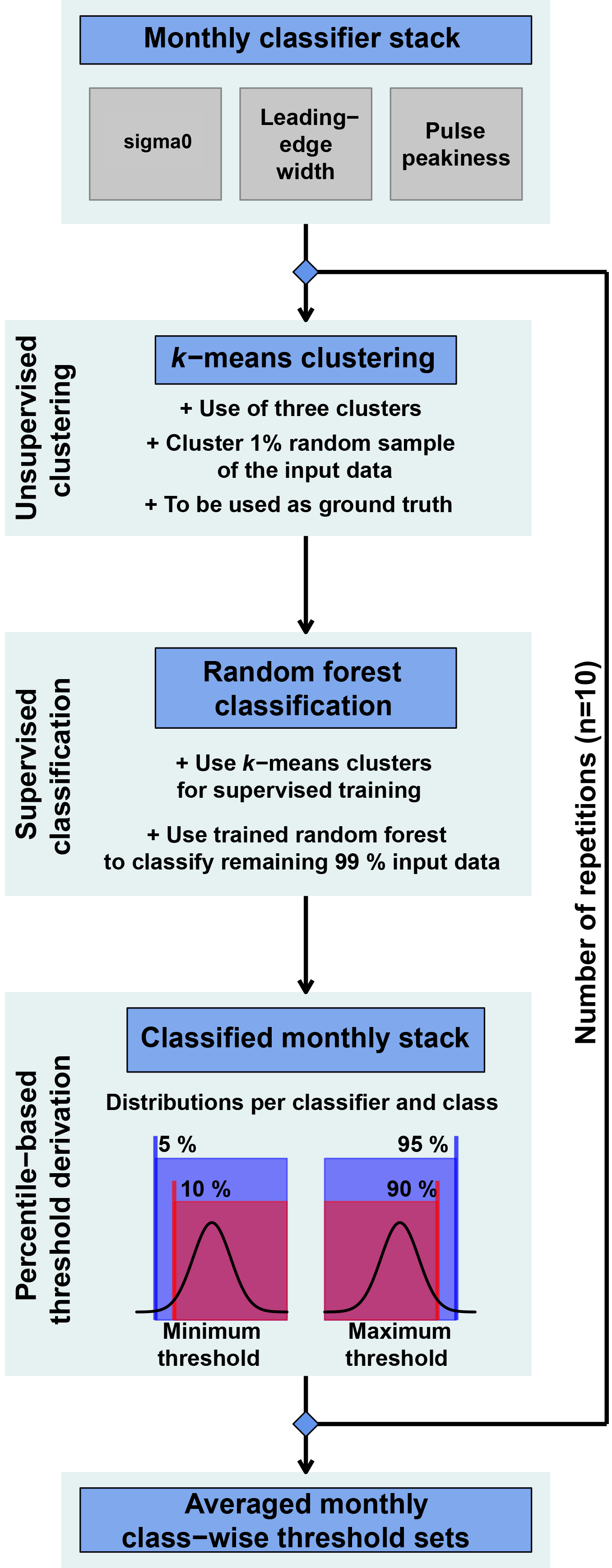
Figure 1Flowchart visualizing the important sub-steps of unsupervised clustering and supervised classification in order to derive the new surface-type thresholds from monthly stacks of surface backscatter, leading-edge width, and pulse peakiness.
Over the course of a winter season, ice conditions can change substantially. Similar to leads, young- and thin-ice areas cause specular reflections compared to other ice types (Zygmuntowska et al., 2013). Furthermore, the amount of leads varies both seasonally and regionally. Based on fixed thresholds for a whole winter season, these changes are difficult to capture, and the rejection rate is increased unnecessarily. Hence, we decided on using monthly thresholds to improve the overall results and data quality.
There is a general lack of ground-truth data as collocated measurements of the same sea-ice situation are very difficult due to sea-ice drift. However, received waveforms have very distinct characteristics and are well described in the literature (Ricker et al., 2014; Schwegmann et al., 2016). These characteristics can also be deduced from the chosen set of classifier parameters. In order to overcome the lack of ground truth, we decided to use a combination of unsupervised clustering and supervised classification.
Based on this combination, we are able to determine suitable thresholds for data acquired by Envisat as well as CryoSat-2. The workflow of how we derived the surface-type thresholds is summarized in Fig. 1 and described thoroughly in the following subsections.
2.2.2 Monthly classifier parameters and k-means clustering
In a first step, the three classifier parameters of surface backscatter, pulse peakiness, and leading-edge width are computed for all available L1b data per sensor and month in the MOP from November 2010 to March 2012.
We only use waveforms that are located between 70 and 81.5 ∘N for the Arctic and feature a minimum sea-ice concentration of 70 %. The northern limit of 81.5 ∘N was chosen to assure a maximum of consistency between Envisat and CryoSat-2 with their differing orbital parameters. Until an update to the geographic mode mask in July 2014, CryoSat-2 operated in SIN mode within the area of 80–85 ∘N, 100–140 ∘W (referred to as the “Wingham box”). For this area, as well as all other Arctic areas that are covered while CryoSat-2 operates in SIN mode, we use all waveforms acquired north of 70 ∘N. For the Antarctic the same restrictions apply, but waveforms are geographically limited to an area south of 65 ∘S to exclude the majority of the marginal-ice zone (MIZ) to reduce the impact of ocean swell.
Next, a subset of 1 % is sampled at random without replacement (i.e., each original waveform with corresponding surface backscatter, pulse peakiness, and leading-edge width can only appear once) for each month in the MOP and for each sensor independently. This data sample is then separated into three clusters using an unsupervised methodology named k-means clustering (Hartigan and Wong, 1979; MacQueen, 1967). This unsupervised method (i.e., without any a priori information about the data) is widely used to separate input data of N observations into k clusters of equal variance – in our case, based on the input classifier parameters of surface backscatter, pulse peakiness, and leading-edge width, whereby the within-cluster sum of squares is iteratively minimized (Hartigan and Wong, 1979; MacQueen, 1967). The result is a “labeled” data set where each input waveform with corresponding surface backscatter, pulse peakiness, and leading-edge width is labeled as a sea-ice-type, lead-type, or ambiguous-type waveform.
Generally, the preselection of the number of clusters can be a problem when utilizing k-means clustering. However, while we tested a higher number of initial clusters with the perspective of a later reunion of similar clusters, a separation into just three clusters turned out to be sufficient. Overall, lead waveforms account for a smaller fraction of the total measurements than sea-ice waveforms. Because of this and the fact that k-means clustering tends towards generating equal-size clusters (this is a presumption of k-means clustering algorithms), sole use of k-means clustering for the complete data set was not feasible.
2.2.3 Random-forest classification
As k-means clustering can not be used for classification of the complete data set due to its unevenly distributed nature, the initially clustered 1 % data sample is instead used as a priori information (i.e., a training data set of classified waveforms as sea ice, leads, or ambiguous) for a supervised classification. In our case, we use an ensemble supervised machine-learning method called random forest (Breiman, 2001).
Random forests are based on multiple decision trees. A decision tree is a rather simple statistical tool to predict data categories based on thresholds. Over several steps, the input data set is split at each step (called a “node”) based on a threshold of a given parameter until all input data are categorized. When visualized, a decision tree resembles a tree with an increasing numbers of branches, leading to the final categories (Breiman, 2001).
The procedure of fitting all single decision trees to the random sub-samples is called training. During this training, each decision tree in the random forest is grown following certain rules (Breiman, 2001):
-
First, from the training data of size N, N cases are sampled randomly with replacement as a “new” and specific training data set for each single tree. This means that the resulting “new” training data set for each tree has the same size as the input training data, but any single waveform with corresponding surface backscatter, pulse peakiness, and leading-edge width can appear multiple times (i.e., “with replacement”).
-
Second, for M input parameters (in our case surface backscatter, pulse peakiness, and leading-edge width), Breiman (2001) states that ideally a fixed number m ≪ M of the given input parameters is specified and randomly selected out of M. The best split on these selected parameters m is then used to split the node. Throughout the growth of the forest, the value of m is held constant.
-
Third, each tree is grown out fully, i.e., to its largest possible extent. No pruning is applied. In contrast to single decision trees that tend to overfit (i.e., match data too precisely and therefore fail for any additional data), random forests do not overfit and are also capable of dealing with unbalanced data sets (Breiman, 2001).
For our purpose, we always grow a total number of 500 decision trees per training in each month. Due to the small number of input parameters (M=3), we set m to 1, following the suggestion by Breiman (2001) to approximate m by .
The result is an ensemble of 500 single uncorrelated decision-tree classifiers called a random forest (Breiman, 2001). After initial training, the random forest can be used for classification of the remaining 99 % of the initial monthly data. During this classification, each decision tree in the now-trained random forest categorizes each waveform based on surface backscatter, pulse peakiness, and leading-edge width into a sea-ice-type, a lead-type, or an ambiguous-type waveform. In the end, the majority of all decision trees in the random forest decides the resulting class.
Available data from months that are covered twice during the mission-overlap period are merged for the random-forest training. The trained random forest for each month is then used to classify the remaining 99 % of the corresponding monthly data. From this classified data set, distributions for each of the three classifier parameters for each month in the mission-overlap period are obtained. These distributions feature clear distinctions for each surface-type class (leads, sea ice, and ambiguous). For example, leads in general feature high values in surface backscatter and pulse peakiness as well as shorter leading-edge widths. The opposite can be seen for sea ice. The class of ambiguous signals is placed in between.
2.2.4 Percentile-based averaged thresholds
Thresholds are then obtained from the resulting classifier-parameter distributions by using either the 5th or 10th percentile for a minimum threshold, or the 90th or 95th percentile in the case of a maximum threshold (Fig. 1). The exact numbers were chosen arbitrarily after visual screening of all resulting classifier-parameter distributions to eliminate outliers. The choice of using the more strict (10th/90th) or less strict (5th/95th) percentile thresholds depends on the sensor. Due to its larger footprint and therefore an expected higher degree of surface-type mixing, we chose the more strict thresholds for Envisat and the less strict thresholds for CryoSat-2 due to its smaller footprint.
The decision of whether to derive a minimum or maximum threshold depends on the surface-type class. For example, lead-type waveforms are generally characterized by high values in pulse peakiness as well as surface backscatter due to their specular reflection. Lead-type waveforms therefore feature a very steep increase in echo power which results in short leading-edge widths. Hence, the 5th/10th percentiles of the surface backscatter and pulse-peakiness distributions would be used alongside the 90th/95th percentile of the leading-edge-width distribution. Sea-ice-type waveforms on the other hand should have smaller values in pulse peakiness. Due to their rather diffuse reflection, sea-ice-type waveforms also feature low backscatter and a less steep increase in echo power, which results in longer leading-edge widths. As a result, the 90th/95th percentiles are used for the surface backscatter and pulse-peakiness distributions. For the leading-edge width, the 5th/10th percentile of its distribution is used. As we positively identify sea-ice and lead waveforms from all available measurements using these thresholds, all remaining waveforms are classified as ambiguous.
Additionally, for all classifications of leads as well as sea ice in both hemispheres we set a minimum requirement of 70 % sea-ice concentration.
The whole procedure, starting with randomly sampling 1 % from the initial monthly stack, is then repeated 10 times. As the whole procedure is initially based on random sampling, this repetition is done to compensate for the odd case of an insufficient representation of lead or sea-ice waveforms in the sampled data. In a last step, the average minimum/maximum thresholds for each classifier parameter, surface-type class, and month in the MOP are estimated for each sensor. These thresholds are summarized in Tables A1–A6 in the Appendix.

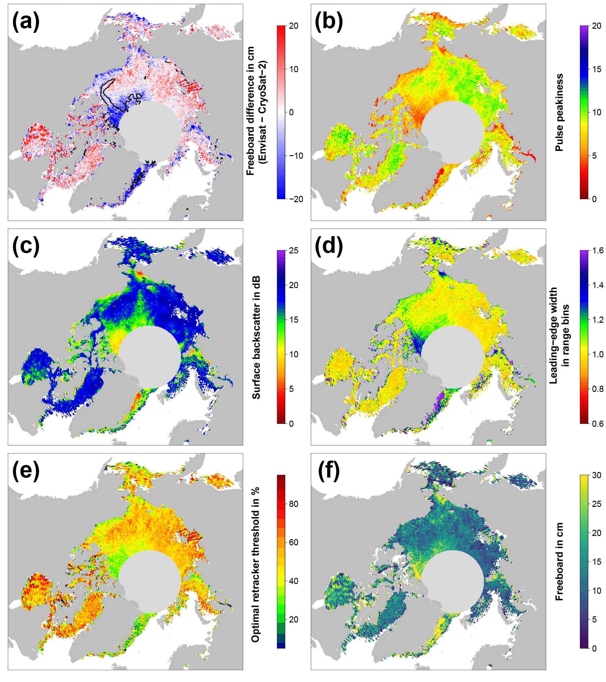
Figure 2Exemplary visualizations of freeboard differences between Envisat and CryoSat-2 (a, in cm; the black isoline resembles the boundary of 75 % multi-year-ice fraction), Envisat pulse peakiness (b, unitless), Envisat surface backscatter (c, in dB), Envisat leading-edge width (d, in range bins), optimal retracker threshold (e, in %), and the resulting Envisat freeboard using our adaptive retracker procedure (f; in cm) for the Arctic in November 2011.
2.3 Range retracking and freeboard retrieval
The range-retracking algorithm for Envisat and CryoSat-2 waveforms is identical for sea-ice-type and lead-type waveforms. The TFMRA used (Helm et al., 2014; Ricker et al., 2014) is based on the following steps:
-
either estimating the noise level as the average of the first five bins of the waveform (CryoSat-2) or discarding all counts in the first five bins of the waveform as these just contain artifacts of the fast Fourier transformation (Envisat);
-
oversampling of the waveforms by a factor of 10 using linear interpolation;
-
smoothing of the oversampled waveforms with a running-mean window-filter size of 11 (Envisat, CryoSat-2 SAR) or 21 (CryoSat-2 SIN) range bins;
-
locating the first local maximum of the waveform, which has to be higher than the noise level by 15 % of the absolute peak power;
-
obtaining the range value (i.e., the elevation) at a specified percentage threshold of the power at the detected first maximum, by linear interpolation of the smoothed and oversampled waveform.
The conversion from range estimates into sea-ice freeboard follows by subtracting the interpolated sea-surface height (the sum of mean sea-surface height taken from the DTU2015 product and the instantaneous sea-surface height anomaly estimated from the interpolated elevation between present leads) at the floe location from the elevation of the sea-ice floe. Given a wave-propagation speed correction based on the auxiliary snow-depth data, sea-ice freeboard can be calculated. A thorough description of the calculation of sea-ice freeboard (and also sea-ice thickness, which is not part of this study) is described in Ricker et al. (2014).
Continuing on the last point of the general TFMRA retracking procedure, the choice of retracker threshold is pivotal for the range estimation. Following the Alfred Wegener Institute (AWI)'s implementation for CryoSat-2 (Ricker et al., 2014), we use a threshold of 50 % from the first-maximum peak power both for lead-type and sea-ice-type waveforms. For pulse-limited altimetry such as Envisat, retracking near the maximum power for leads proved to be essential to retrieve reasonable sea-ice freeboard estimates (Giles et al., 2007). Hence, we chose a threshold of 95 % for leads from Envisat waveforms. In a very recent study by Guerreiro et al. (2017), the use of 50 % for lead-type waveforms resulted in initial average conditions where the lead surface elevation was detected above that of the surrounding sea-ice floes. When we used a single fixed threshold for the range retrieval over sea ice similar to that for CryoSat-2 (i.e., a 50 % threshold from the first local maximum peak power), our Envisat sea-ice freeboard estimates featured an overall smaller variation and range compared to CryoSat-2 estimates. We relate this behavior to the much larger footprint and the therefore increased mixing of surface types of different surface-roughness scales in every obtained Envisat waveform.
We used our methodology as illustrated in the previous paragraphs and in Fig. 1 to compute the sea-ice freeboard for every month of the MOP separately for Envisat and CryoSat-2. Subsequently, we computed the sea-ice freeboard difference of Envisat minus CryoSat-2, which is shown together with parameters of the retrieval in Figs. 2 and 3. From Figs. 2a and 3a it appears that there are substantial differences in the resulting sea-ice freeboard between both sensors. However, these patterns of sea-ice freeboard differences are related to differences in the Envisat waveform parameters of pulse peakiness, surface backscatter, and leading-edge width (Figs. 2b–d and 3b–d). These waveform parameter variations in turn reflect changes in the surface properties. Areas of MYI near the Canadian Archipelago and areas influenced by MYI export are in general substantially thinner for Envisat than CryoSat-2 (e.g., about 20 cm or more in March, Fig. 3a). On the other side, areas of predominantly FYI are in general thicker in the Envisat data (Fig. 2a). However, the level of freeboard difference is not constant throughout a winter season but rather appears to be seasonal, where Envisat appears to be unable to keep track of these seasonal changes.

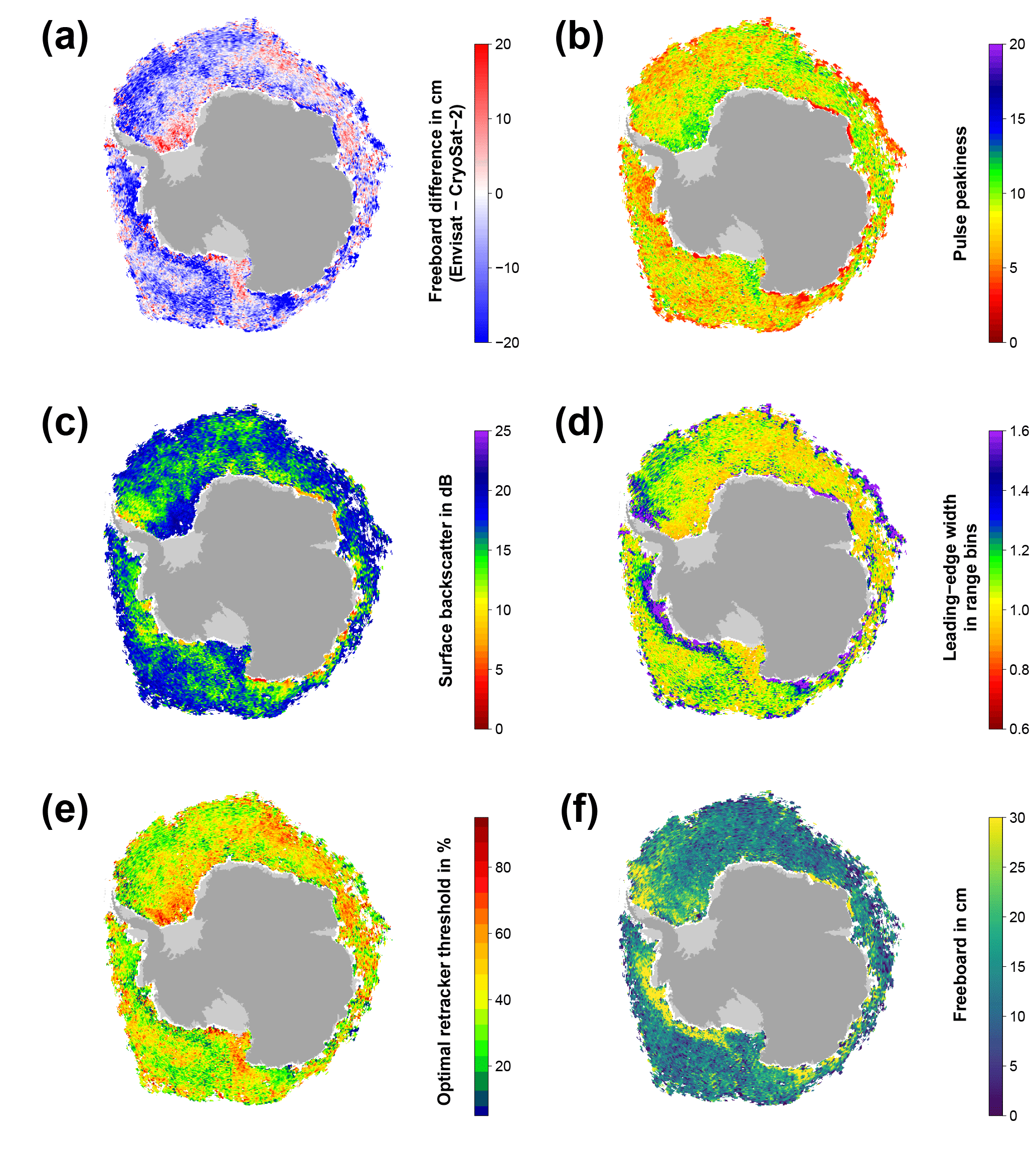
Figure 5Exemplary visualizations for the Antarctic in September 2011 in the same setup as Fig. 2.
As these differences in sea-ice freeboard between CryoSat-2 and Envisat appear to be indeed strongly correlated with patterns in the surface backscatter and the leading-edge width of Envisat waveforms (Figs. 2c–d and 3c–d), we decided to apply a novel empirical tuning scheme by computing an adaptive range-retracker threshold as a function of surface backscatter and the leading-edge width to mitigate the differences. Due to the already-mentioned larger footprint of Envisat and hence increased mixing of different surface types, it appears to be necessary to treat waveforms differently according to the waveform shape (and hence surface properties) by means of retracking the main scattering horizon. Guerreiro et al. (2017) proposed in their study a correction scheme deriving a relationship between monthly-gridded pulse peakiness and the monthly-gridded freeboard differences between CryoSat-2 and Envisat based on a third-order polynomial fit. In contrast to applying a similar post-retracking correction to the resulting freeboard estimates, we apply our correction already during waveform retracking.
In order to derive a functional relationship between retracker threshold and surface backscatter/leading-edge width, we first processed all available Envisat data for the complete MOP. This processing was done using the TFMRA with a fixed threshold for leads of 95 % and a threshold for sea-ice-type waveforms that was changed in each run. This sea-ice threshold ranged between 5 % and 95 % in steps of 5 %. For example, in the first run the complete data set was processed using a retracker threshold of 5 % for sea-ice-type waveforms, and the resulting sea-ice freeboard was calculated. In the next run, a fixed threshold of 10 % was used for all sea-ice-type waveforms and so on. This continued until the last run was computed with a retracker threshold of 95 % for sea-ice-type waveforms and the resulting sea-ice freeboard was calculated.
From this data set, the optimal threshold, i.e., the threshold that yields the smallest absolute difference in sea-ice freeboard between Envisat and CryoSat-2, was iteratively derived. Exemplary results are shown in Figs. 2e and 3e. Again, the seasonal change observed in the waveform parameters is also reflected in the resulting optimal-threshold values. These show a varying range of optimal-threshold values that are in general higher for the early winter compared to the late winter.
In the next step, we derive a functional relationship between optimal-threshold values and the waveform parameters of surface backscatter and leading-edge width for our adaptive threshold range retracking. Therefore, we first average all optimal-threshold values during the MOP for bins of 0.25 dB for the surface backscatter and 0.025 for the leading-edge width. Here, we use a three-dimensional coordinate system with average optimal threshold (z axis) against leading-edge width (x axis) and surface backscatter (y axis).
The months November through March are covered twice during the MOP, and both occurrences were used. October and April, which were only covered once during the MOP, were each added twice to circumvent issues of under-representation in their number of data values added to the total.
Through this compilation of monthly data points, three third-order polynomial planes were fitted based on different weighting schemes in order to maximize the adjusted coefficient of determination (). is a measure for the quality of the model fit. In contrast to the normal R2, decreases through adding useless predictors to a model and is therefore a more robust measure for model quality than the standard R2. As weights, we used the number of optimal-threshold values per bin in the x–y plane, the inverse standard deviation of all optimal-threshold values per bin (1∕σ), or no weights at all.
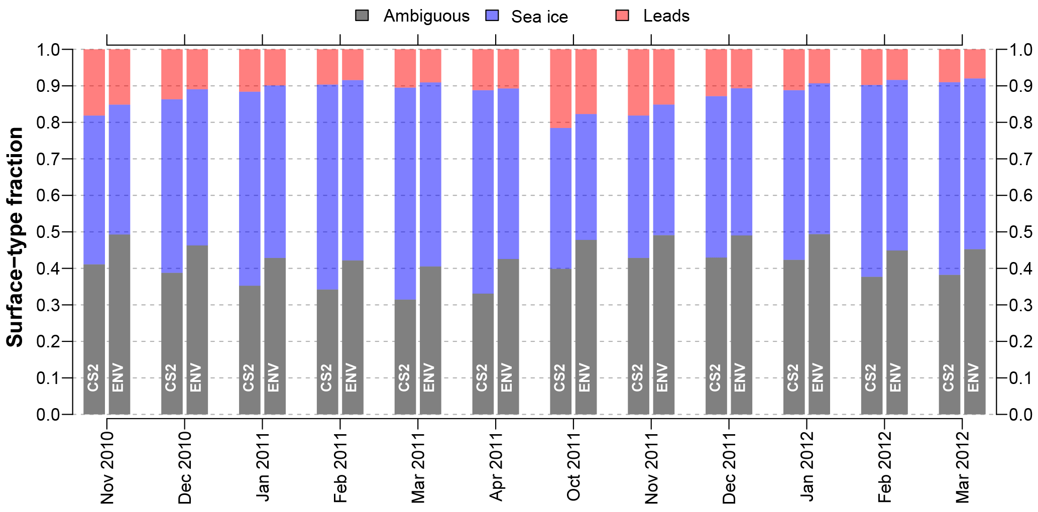
Figure 6Time series of surface-type fractions for the mission-overlap period between CryoSat-2 (CS2) and Envisat (ENV) for the Arctic based on orbit-track (i.e., non-gridded) data.
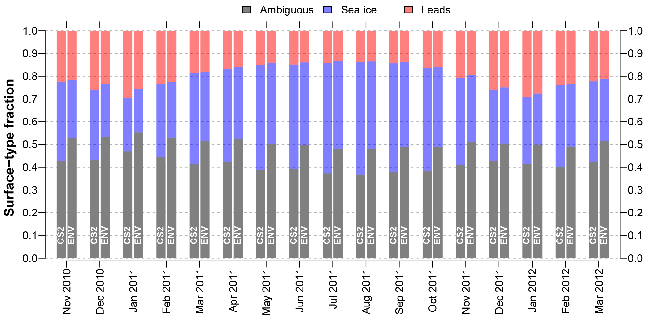
Figure 7Time series of surface-type fractions for the mission-overlap period between CryoSat-2 (CS2) and Envisat (ENV) for the Antarctic based on orbit-track (i.e., non-gridded) data.
The optimal threshold (thopt, in decimal values) to be used in the adaptive range retracking for the Arctic as a function of surface backscatter (σo) and leading-edge width (lew) is given by Eq. (2):
For the Arctic, Eq. (2) achieved the highest adjusted of 0.94 with the inverse standard deviation as weights. All data points used have a minimum of 50 occurrences to reduce noise and were obtained in the central Arctic only (i.e., we excluded not only the Canadian Arctic Archipelago and the Hudson Bay but also extensive fast-ice areas like the Laptev Sea). The resulting monthly-gridded Envisat freeboard estimates are shown in Figs. 2f and 3f.
In a first attempt, we applied Eq. (2) also to the Southern Hemisphere. However, this did not result in an improvement of the freeboard differences between Envisat and CryoSat-2. The reason for that can partly be seen in Figs. 4 and 5.
In contrast to the Arctic (Figs. 2 and 3), there is less seasonality in the data; i.e., the differences between early and late winter are less prominent in the sea-ice freeboard differences as well as the optimal-threshold values. Overall, a wider range of optimal-threshold values is necessary in any given month, in order to achieve a minimum freeboard difference (Figs. 4e and 5e).
Additionally, the overall range and distribution of the surface backscatter is different between the Arctic and the Antarctic (not shown), and patterns in surface backscatter and leading-edge width are less correlated in some areas (e.g., the MIZ as well as in the central Weddell Sea; Figs. 4c–d and 5c–d). This is potentially related to ice–snow interface flooding paired with subsequent refreezing and formation of snow ice, large fast-ice areas with a different snow stratigraphy and depth, and a different ice-growth history than in the Arctic, causing a larger fraction of rough and deformed sea ice.
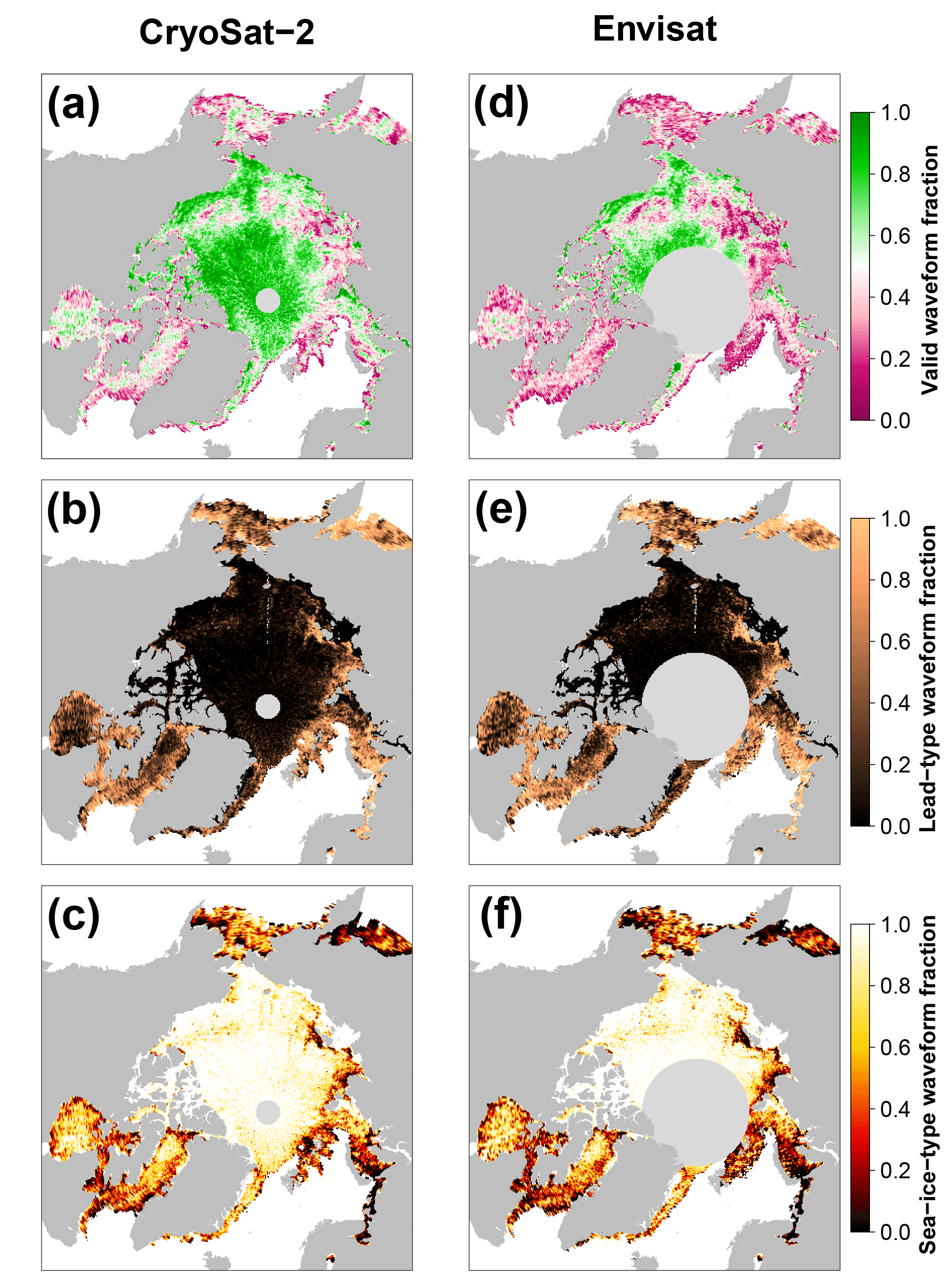
Figure 8Comparison of gridded surface-type classification benchmarks of valid waveform fractions (a, d; ratio of either lead-type or sea-ice-type classification to the total number of waveforms per grid cell), lead-type waveform fraction (b, e; ratio of lead-type classifications to the number of valid classifications per grid cell), and the sea-ice-type waveform fraction (c, f; ratio of sea-ice-type classifications to the number of valid classifications per grid cell) between CryoSat-2 and Envisat for March 2012 in the Arctic.
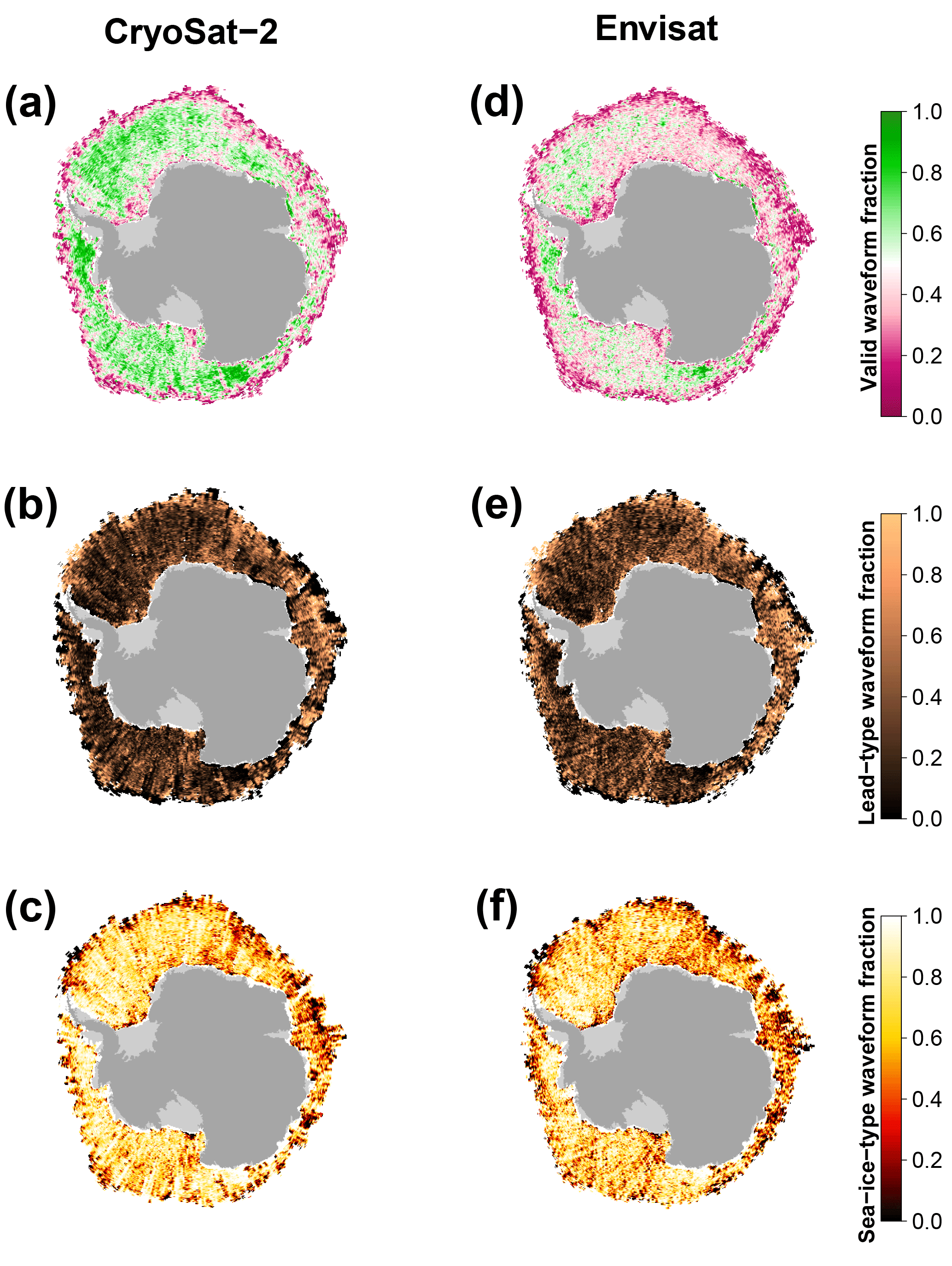
Figure 9Comparison of gridded surface-type classification benchmarks in the same setup as Fig. 8 between CryoSat-2 and Envisat for September 2011 in the Antarctic.
For the Antarctic, a second-order polynomial fit resulted in the best statistical result ( of 0.77) to describe the optimal threshold as a function of leading-edge width and surface backscatter. Equation (3) summarizes the relationship for deriving the optimal threshold (thopt, in decimal values) in the Antarctic as a function of surface backscatter (σo) and leading-edge width (lew):
Here, the best fit is obtained using the total number of optimal-threshold values per bin as weights. All data points used also have a minimum of 50 occurrences and were obtained by excluding ice zones around the Antarctic that appear to be influenced by ocean swell (identified by surface backscatter and/or leading edge with outlier artifacts) as well as the months from December through April.
Utilizing both equations, for each range retracking of every sea-ice waveform, the to-be-used threshold is calculated from the waveform-associated surface backscatter and leading-edge-width value. This threshold is then believed to yield the mean-scattering surface in best accordance to the CryoSat-2 measurements. The resulting monthly-gridded Envisat freeboard estimates are shown in Figs. 4f and 5f.
In this section we want to present and discuss the results obtained for the MOP between Envisat and CryoSat-2. This is presented first for the surface-type classification and then for the range retracking and the associated sea-ice freeboard retrieval.
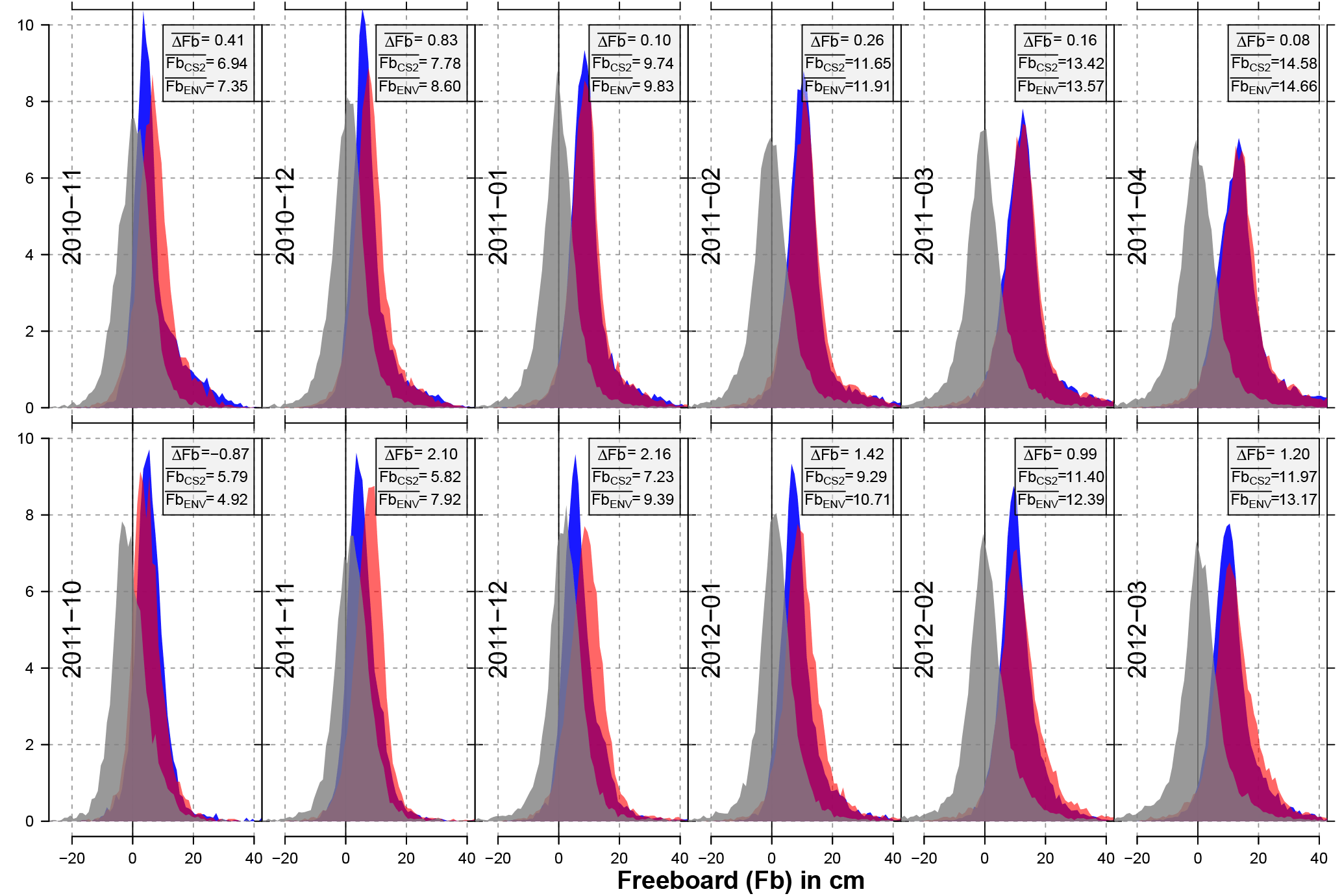
Figure 10Histograms of freeboard for each month of the mission-overlap period (in centimeters) for Envisat (red) and CryoSat-2 (blue) as well as the corresponding freeboard difference between both sensors (gray) for the Arctic. Furthermore, the average freeboard difference (; Envisat minus CryoSat-2), and the average freeboards for CryoSat-2 () and Envisat () are given in centimeters in the gray box for each month.

Figure 11Histograms of freeboard for each month of the mission-overlap period (in centimeters) for Envisat (red) and CryoSat-2 (blue) as well as the corresponding freeboard difference between both sensors (gray) for the Antarctic. Furthermore, the average freeboard difference (; Envisat minus CryoSat-2), and the average freeboards for CryoSat-2 () and Envisat () are given in centimeters in the gray box for each month.
3.1 Surface-type classification
Utilizing our surface-type classification scheme results in an overall much better agreement between CryoSat-2 and Envisat based on lead, sea-ice, and valid fractions (Figs. 6–9). Compared to the surface-type classification used during SICCI-1 for Envisat, our approach is less strict and allows for substantially more waveforms being classified as either lead or sea-ice type that were rejected before. Additionally, a very high fraction of lead detections was present, compared to only a very small fraction of classified sea-ice-type waveforms during SICCI-1 (Schwegmann et al., 2016). Furthermore, the inter-mission consistency of the surface-type classification for the Arctic as well as the Antarctic has improved substantially (Figs. 8 and 9).
The increased number of valid waveforms has an additional positive side effect on the overall data record: it allows for a much finer grid resolution to be used in the final Level 3 product without any concessions on overall coverage. Here, we are now able to provide a 25 km × 25 km (50 km × 50 km) resolution gridded data set for the Arctic (Antarctic) compared to the 100 km × 100 km during SICCI-1.
Direct comparisons of surface-type class fractions (i.e., ambiguous, lead, or sea-ice type) over the course of the MOP reveal an overall good agreement between CryoSat-2 and Envisat based on the non-gridded orbit data (Figs. 6 and 7). While the fractions of lead and sea-ice waveforms are on average slightly smaller for Envisat compared to CryoSat-2 (about 8 % for the Arctic and 10 % for the Antarctic), both sensors show a similar seasonal development in both hemispheres. Especially, the fraction differences of detected leads are very small with a root-mean-squared difference (RMSD) of 2 % and 1 % for the Arctic and Antarctic, respectively. The discrepancy is larger for detected sea-ice waveforms with a RMSD of 6 % for the Arctic and 9 % for the Antarctic.
Exemplary visualizations of monthly-gridded intercomparisons between Envisat and CryoSat-2 based on valid, lead, and sea-ice waveform fractions are shown in Figs. 8 and 9. In these gridded data sets, the overall good agreement is confirmed. On average, the gridded valid waveform fraction for Envisat is 9 % (11 %) lower in the Arctic (Antarctic) than the ones achieved by CryoSat-2. This behavior is expected in regions with high rates of sea-ice dynamics such as the Beaufort Sea, where the increased surface-type mixing from the much larger footprint of Envisat likely prevents a clearer separation between waveform types. Lead and sea-ice fractions differ by 2 % and 4 % for the Arctic and Antarctic, respectively.
Nevertheless, both comparisons highlight the overall good agreement that could be achieved between both sensors with this inter-mission-consistent surface-type classification scheme. These results therefore lay the foundation for a proper inter-mission sea-ice freeboard and sea-ice thickness data record.
3.2 Range retracking and freeboard retrieval
In this subsection, we show and discuss the results of using the adaptive threshold retracker for Envisat. For the Arctic, Fig. 10 shows the histograms of CryoSat-2 (blue) and Envisat (red) freeboards in centimeters as well as the histogram of the resulting freeboard differences (Envisat minus CryoSat-2; gray). Furthermore, average freeboard estimates for all distributions per month during the mission-overlap period for Envisat and CryoSat-2 are shown.
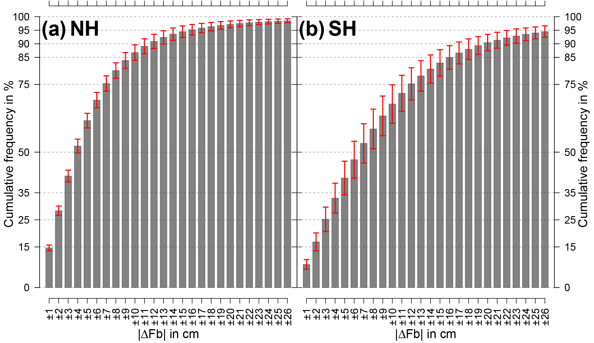
Figure 12Cumulative frequencies of absolute freeboard differences (Envisat minus CryoSat-2) as shown in Figs. 10 and 11 averaged over all months in the MOP. Data are presented for the Northern Hemisphere (a) as well as the Southern Hemisphere (b). Error bars indicate ±1 standard deviation. First bar covers the absolute freeboard difference range from 0 to 1 cm, second bar from 1 to 2 cm, and so on.

While in the first winter season the match is nearly perfect with absolute average freeboard differences below 1 cm, differences during the second winter season increase up to about 3 cm. Nevertheless, this is a substantial improvement over any previous comparisons conducted during SICCI-1. Especially for the Arctic spring period (March and April), differences in average freeboard are 1.2 cm or less. The overall maximum monthly average freeboard differences is 2.2 cm.
A comparison to the results of Guerreiro et al. (2017) is constrained by the different methods used. Besides the pulse-peakiness correction of the Envisat monthly freeboard, Guerreiro et al. (2017) also apply a 25 km along-track median smoothing to all freeboard estimates and afterward discard all freeboard estimates below −1 m and above 2 m. The resulting values are then used to compile the monthly-gridded data set. In this study, we set the lower and upper sea-ice freeboard thresholds to −0.25 and 2.25 m, respectively, without applying any smoothing. Values outside this range are discarded. Furthermore, we also compute freeboard results outside the central Arctic basin and take them into account for our comparison. While the differences between CryoSat-2 and Envisat freeboard appear to be comparable between both studies, the average monthly sea-ice freeboard estimates for both sensors are between about 3 and 10 cm larger in our study compared to the results shown in Guerreiro et al. (2017).
For the Antarctic, results are not as good as for the Arctic (Fig. 11). Overall, the approach has less skill in matching Envisat sea-ice freeboards to the ones of CryoSat-2. This is very likely related to other physical process such as a more complex snow stratigraphy caused by the more strongly varying weather patterns with melt–refreeze cycles even in the middle of winter. Furthermore, snow–ice interface flooding causes a (temporarily) wet and saline basal snow layer and influences the sea-ice surface roughness. However, issues causing these sensor differences are subject to further investigation. Overall, there is a stronger seasonality in the monthly freeboard differences between summer and winter, which also leads towards a higher maximum monthly average freeboard difference of about 2.7 cm.
A different way of visualizing these results is shown in Fig. 12. Here, the cumulative frequencies of absolute freeboard differences (Envisat minus CryoSat-2, i.e., the gray histograms in Figs. 10 and 11) are averaged over the complete MOP for both hemispheres. For the Arctic (Fig. 12a), more than 50 % of all data points are in an absolute freeboard difference range of ±4 cm. Furthermore, more than 75 % (90 %) of all data points are in a range of 12 cm) absolute freeboard difference. However, for the Antarctic (Fig. 12b) results are not as good. In order to achieve values of 50 %, 75 %, and 90 % cumulative frequency, absolute freeboard differences increase to ±7, ±12, and ±20 cm, respectively.
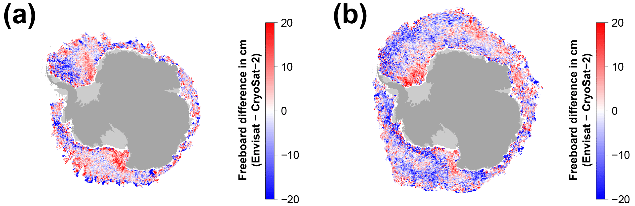
Resulting freeboard differences using our new approach for Envisat and CryoSat-2 are shown in Fig. 13 for the Arctic and in Fig. 14 for the Antarctic. Shown are the same months as in Figs. 2–5. While the overall differences are minimized, especially in the Arctic, there are still areas with rather large freeboard differences. In the Arctic, these comprise the Hudson Bay and the area east of Greenland. In the Antarctic, while the freeboard differences between both sensors are lowered through applying the methodology presented here, the overall resulting differences remain larger than the ones estimated for the Arctic.
This study showed the potential of a combined novel surface-type classification scheme in combination with a waveform-parameter-dependent adaptive threshold retracker approach in order to create a consistent data set of Envisat and CryoSat-2 sea-ice freeboard estimates. This approach is based on the observed correlation between freeboard differences between both sensors and the waveform characteristics of surface backscatter and leading-edge width. Their spatiotemporal variations in acquired Envisat waveforms reflect changes in surface properties such as the surface-roughness- and footprint-size-dependent surface-type mixing. We applied this approach for the mission-overlap period from November 2010 to March 2012 and then used it to iteratively train and apply an adaptive threshold retracker to Envisat for both hemispheres. Different sea-ice conditions in both hemispheres also result in different inter-mission biases between Envisat and CryoSat-2. In contrast to previous attempts during SICCI-1, the inter-mission sea-ice freeboard biases could be minimized.
Furthermore, through the application of our inter-mission-consistent surface-type classification in SICCI-2, a much higher comparability between the amount and location of positively identified lead-type and sea-ice-type waveforms for Envisat and CryoSat-2 could be achieved. Additionally, due to the higher amount of identified waveforms, a resolution of 25 km × 25 km and 50 km ×50 km could be realized in the final gridded data product for the Arctic and Antarctic, respectively. This is a substantial improvement over SICCI-1, where, due to the much stricter surface-type classification and associated low identification/classification rates of waveforms, a resolution of only 100 km × 100 km could be achieved without a substantial drop in spatial data coverage for Envisat.
While the employed surface-type classification is truly consistent between both sensors, there still is an inconsistency with regard to the range retracking in using fixed thresholds for CryoSat-2 in contrast to an adaptive procedure for Envisat. However, the purpose of this study in the framework of SICCI-2 was to use existing data sets and algorithms wherever possible to create a cross-calibrated freeboard algorithm. In the future, we are planning to develop a truly consistent similar adaptive retracking procedure for CryoSat-2 as well. As we take the CryoSat-2 data in this study as correct, the shown evaluation is not independent. A truly independent evaluation will be conducted in a future study.
The next step from this point is to start creating an inter-mission-consistent and reliable climate data record on Arctic and Antarctic sea-ice thickness and volume as well as to investigate interannual and seasonal changes. Moreover, investigation of the stability of assumptions in auxiliary data sets is necessary. Here, especially the validity of the snow-depth climatologies used in the freeboard-to-thickness conversion in a changing Arctic and Antarctic needs to be investigated.
Links to all auxiliary data sets used are provided in the text. ESA SICCI-2 data sets for the Arctic and Antarctic based on the presented methodology are available via the following DOIs:
-
https://doi.org/10.5285/5b6033bfb7f241e89132a83fdc3d5364 (Hendricks et al., 2018a),
-
https://doi.org/10.5285/fbfae06e787b4fefb4b03cba2fd04bc3 (Hendricks et al., 2018b),
-
https://doi.org/10.5285/ff79d140824f42dd92b204b4f1e9e7c2 (Hendricks et al., 2018c),
-
https://doi.org/10.5285/48fc3d1e8ada405c8486ada522dae9e8 (Hendricks et al., 2018d),
-
https://doi.org/10.5285/54e2ee0803764b4e84c906da3f16d81b (Hendricks et al., 2018e),
-
https://doi.org/10.5285/550d938da3184d0ca44a06a4c0c14ffa (Hendricks et al., 2018f),
-
https://doi.org/10.5285/f4c34f4f0f1d4d0da06d771f6972f180 (Hendricks et al., 2018g),
-
https://doi.org/10.5285/b1f1ac03077b4aa784c5a413a2210bf5 (Hendricks et al., 2018h).
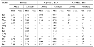
Table A1Pulse-peakiness thresholds for the surface-type classification of lead-type waveforms for Envisat, CryoSat-2 SAR mode, and CryoSat-2 SIN mode data for the Arctic and the Antarctic. Values for the pulse peakiness are unitless.
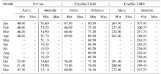
Table A2Surface backscatter thresholds for the surface-type classification of lead-type waveforms for Envisat, CryoSat-2 SAR mode, and CryoSat-2 SIN mode data for the Arctic and the Antarctic. Values for surface backscatter are given in decibels.
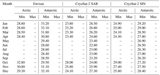
Table A3Leading-edge width thresholds for the surface-type classification of lead-type waveforms for Envisat, CryoSat-2 SAR mode, and CryoSat-2 SIN mode data for the Arctic and the Antarctic. Values are in range-bin fractions for the leading-edge width.
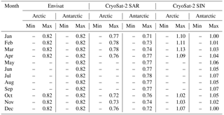
Table A4Pulse-peakiness thresholds for the surface-type classification of sea-ice-type waveforms for Envisat, CryoSat-2 SAR mode, and CryoSat-2 SIN mode data for the Arctic and the Antarctic. Values for the pulse peakiness are unitless.
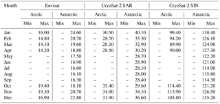
Table A5Surface backscatter thresholds for the surface-type classification of sea-ice-type waveforms for Envisat, CryoSat-2 SAR mode, and CryoSat-2 SIN mode data for the Arctic and the Antarctic. Values for surface backscatter are given in decibel.
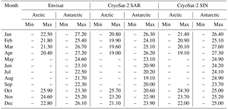
Table A6Leading-edge width thresholds for the surface-type classification of sea-ice-type waveforms for Envisat, CryoSat-2 SAR mode, and CryoSat-2 SIN mode data for the Arctic and the Antarctic. Values are in range-bin fractions for the leading-edge width.
SP designed the surface-type classification as well as the adaptive retracker approach, conducted the analysis, and drafted the original manuscript. SH developed pySIRAL and assisted with the analysis, the approach development, and the data processing using pySIRAL. RR, SK, and ER assisted in the analysis as well as in writing the manuscript.
The authors declare no conflict of interests.
This work was funded through the ESA Climate Change Initiative. The authors
would like to thank the International Space Science Institute (ISSI Bern) for
its support to an international team focused on current scientific issues
in the observation of sea level and sea ice at polar latitudes, which
fostered fruitful discussion on the ideas for this paper. Furthermore, the
valuable comments of three reviewers (Thomas Armitage, Nathan Kurtz, and
Sara Fleury) as well as editor Jennifer Hutchings are very much appreciated
and greatly improved this paper.
The
article processing charges for this open-access
publication
were covered by a Research
Centre of the Helmholtz
Association.
Edited by: Jennifer
Hutchings
Reviewed by: Nathan Kurtz, Thomas Armitage, and Sara
Fleury
Andersen, O., Knudsen, P., and Stenseng, L.: The DTU13 MSS (Mean Sea Surface) and MDT (Mean Dynamic Topography) from 20 Years of Satellite Altimetry, in: IGFS 2014, Springer International Publishing, Cham, 111–121, 2016. a
Armitage, T. W. K. and Davidson, M. W. J.: Using the Interferometric Capabilities of the ESA CryoSat-2 Mission to Improve the Accuracy of Sea Ice Freeboard Retrievals, IEEE T. Geosci. Remote, 52, 529–536, 2014. a
Armitage, T. W. K. and Ridout, A. L.: Arctic sea ice freeboard from AltiKa and comparison with CryoSat-2 and Operation IceBridge, Geophys. Res. Lett., 42, 6724–6731, https://doi.org/10.1002/2015GL064823, 2015. a
Behrendt, A., Dierking, W., Fahrbach, E., and Witte, H.: Sea ice draft in the Weddell Sea, measured by upward looking sonars, Earth Syst. Sci. Data, 5, 209–226, https://doi.org/10.5194/essd-5-209-2013, 2013. a
Breiman, L.: Random Forests, Mach. Learn., 45, 5–32, https://doi.org/10.1023/A:1010933404324, 2001. a, b, c, d, e, f, g
Cavalieri, D. J., Parkinson, C. L., Gloersen, P., Comiso, J. C., and Zwally, H. J.: Deriving long-term time series of sea ice cover from satellite passive-microwave multisensor data sets, J. Geophys. Res., 104, 15803–15814, https://doi.org/10.1029/1999JC900081, 1999. a
Comiso, J. C.: Large Decadal Decline of the Arctic Multiyear Ice Cover, J. Climate, 25, 1176–1193, https://doi.org/10.1175/JCLI-D-11-00113.1, 2012. a, b
Connor, L. N., Laxon, S. W., Ridout, A. L., Krabill, W. B., and McAdoo, D. C.: Comparison of Envisat radar and airborne laser altimeter measurements over Arctic sea ice, Remote Sens. Environ., 113, 563–570, https://doi.org/10.1016/j.rse.2008.10.015, 2009. a
Farrell, S. L., Laxon, S. W., McAdoo, D. C., Yi, D., and Zwally, H. J.: Five years of Arctic sea ice freeboard measurements from the Ice, Cloud and land Elevation Satellite, J. Geophys. Res., 114, C04008, https://doi.org/10.1029/2008JC005074, 2009. a
Frost, T., Kern, S., and Heygster, G.: Passive microwave snow depth on Antarctic sea ice assessment, ESA CCI Sea-Ice ECV project report SICCI-ANT-PMW-SDASS-11-14, version 1.1, 2015. a
Giles, K., Laxon, S., Wingham, D., Wallis, D., Krabill, W., Leuschen, C., McAdoo, D., Manizade, S., and Raney, R.: Combined airborne laser and radar altimeter measurements over the Fram Strait in May 2002, Remote Sens. Environ., 111, 182–194, https://doi.org/10.1016/j.rse.2007.02.037, 2007. a, b, c
Guerreiro, K., Fleury, S., Zakharova, E., Kouraev, A., Rémy, F., and Maisongrande, P.: Comparison of CryoSat-2 and ENVISAT radar freeboard over Arctic sea ice: toward an improved Envisat freeboard retrieval, The Cryosphere, 11, 2059–2073, https://doi.org/10.5194/tc-11-2059-2017, 2017. a, b, c, d, e
Haas, C.: Evaluation of ship-based electromagnetic-inductive thickness measurements of summer sea-ice in the Bellingshausen and Amundsen Seas, Antarctica, Cold Reg. Sci. Technol., 27, 1–16, https://doi.org/10.1016/S0165-232X(97)00019-0, 1998. a
Haas, C., Nicolaus, M., Willmes, S., Worby, A., and Flinspach, D.: Sea ice and snow thickness and physical properties of an ice floe in the western Weddell Sea and their changes during spring warming, Deep-Sea Res. Pt. II, 55, 963–974, https://doi.org/10.1016/j.dsr2.2007.12.020, 2008. a
Hartigan, J. A. and Wong, M. A.: Algorithm AS 136: A K-Means Clustering Algorithm, J. Roy. Stat. Soc. C, 28, 100–108, https://doi.org/10.2307/2346830, 1979. a, b
Helm, V., Humbert, A., and Miller, H.: Elevation and elevation change of Greenland and Antarctica derived from CryoSat-2, The Cryosphere, 8, 1539–1559, https://doi.org/10.5194/tc-8-1539-2014, 2014. a, b
Hendricks, S., Paul, S., and Rinne, E.: ESA Sea Ice Climate Change Initiative (Sea_Ice_cci): Northern hemisphere sea ice thickness from CryoSat-2 on the satellite swath (L2P), v2.0, Centre for Environmental Data Analysis, https://doi.org/10.5285/5b6033bfb7f241e89132a83fdc3d5364, 2018a. a
Hendricks, S., Paul, S., and Rinne, E.: ESA Sea Ice Climate Change Initiative (Sea_Ice_cci): Southern hemisphere sea ice thickness from CryoSat-2 on the satellite swath (L2P), v2.0, Centre for Environmental Data Analysis, https://doi.org/10.5285/fbfae06e787b4fefb4b03cba2fd04bc3, 2018b. a
Hendricks, S., Paul, S., and Rinne, E.: ESA Sea Ice Climate Change Initiative (Sea_Ice_cci): Northern hemisphere sea ice thickness from the CryoSat-2 satellite on a monthly grid (L3C), v2.0, Centre for Environmental Data Analysis, https://doi.org/10.5285/ff79d140824f42dd92b204b4f1e9e7c2, 2018c. a
Hendricks, S., Paul, S., and Rinne, E.: ESA Sea Ice Climate Change Initiative (Sea_Ice_cci): Southern hemisphere sea ice thickness from the CryoSat-2 satellite on a monthly grid (L3C), v2.0, Centre for Environmental Data Analysis, https://doi.org/10.5285/48fc3d1e8ada405c8486ada522dae9e8, 2018d. a
Hendricks, S., Paul, S., and Rinne, E.: ESA Sea Ice Climate Change Initiative (Sea_Ice_cci): Northern hemisphere sea ice thickness from Envisat on the satellite swath (L2P), v2.0, Centre for Environmental Data Analysis, https://doi.org/10.5285/54e2ee0803764b4e84c906da3f16d81b, 2018e. a
Hendricks, S., Paul, S., and Rinne, E.: ESA Sea Ice Climate Change Initiative (Sea_Ice_cci): Southern hemisphere sea ice thickness from Envisat on the satellite swath (L2P), v2.0, Centre for Environmental Data Analysis, https://doi.org/10.5285/550d938da3184d0ca44a06a4c0c14ffa, 2018f. a
Hendricks, S., Paul, S., and Rinne, E.: ESA Sea Ice Climate Change Initiative (Sea_Ice_cci): Northern hemisphere sea ice thickness from the Envisat satellite on a monthly grid (L3C), v2.0, Centre for Environmental Data Analysis, https://doi.org/10.5285/f4c34f4f0f1d4d0da06d771f6972f180, 2018g. a
Hendricks, S., Paul, S., and Rinne, E.: ESA Sea Ice Climate Change Initiative (Sea_Ice_cci): Southern hemisphere sea ice thickness from the Envisat satellite on a monthly grid (L3C), v2.0, Centre for Environmental Data Analysis, https://doi.org/10.5285/b1f1ac03077b4aa784c5a413a2210bf5, 2018h. a
Kern, S. and Ozsoy-Çiçek, B.: Satellite Remote Sensing of Snow Depth on Antarctic Sea Ice: An Inter-Comparison of Two Empirical Approaches, Reomte Sens., 8, 450, https://doi.org/10.3390/rs8060450, 2016. a
Kern, S., Frost, T., and Heygster, G.: Antarctic AMSR-E snow depth product user guide, ESA CCI Sea-Ice ECV project report SICCI-ANT-SD-PUG-14-08, version 2.1, 2015. a
Kern, S., Ozsoy-Çiçek, B., and Worby, P. A.: Antarctic Sea-Ice Thickness Retrieval from ICESat: Inter-Comparison of Different Approaches, Remote Sens., 8, 538, https://doi.org/10.3390/rs8070538, 2016. a
Kurtz, N. T. and Farrell, S. L.: Large-scale surveys of snow depth on Arctic sea ice from Operation IceBridge, Geophys. Res. Lett., 38, L20505, https://doi.org/10.1029/2011GL049216, 2011. a
Kurtz, N. T. and Markus, T.: Satellite observations of Antarctic sea ice thickness and volume, J. Geophys. Res., 117, C08025, https://doi.org/10.1029/2012JC008141, 2012. a
Kwok, R. and Cunningham, G. F.: Variability of Arctic sea ice thickness and volume from CryoSat-2, Phil. Trans. R. Soc. A, 373, 20140157, https://doi.org/10.1098/rsta.2014.0157, 2015. a
Kwok, R. and Rothrock, D. A.: Decline in Arctic sea ice thickness from submarine and ICESat records: 1958–2008, Geophys. Res. Lett., 36, L15501, https://doi.org/10.1029/2009GL039035, 2009. a
Kwok, R., Cunningham, G. F., Wensnahan, M., Rigor, I., Zwally, H. J., and Yi, D.: Thinning and volume loss of the Arctic Ocean sea ice cover: 2003–2008, J. Geophys. Res., 114, C07005, https://doi.org/10.1029/2009JC005312, 2009. a
Laxon, S.: Sea ice altimeter processing scheme at the EODC, International J. Remote Sens., 15, 915–924, https://doi.org/10.1080/01431169408954124, 1994. a
Laxon, S., Peacock, N., and Smith, D.: High interannual variability of sea ice thickness in the Arctic region, Nature, 425, 947–950, https://doi.org/10.1038/nature02050, 2003. a, b, c
Laxon, S. W., Giles, K. A., Ridout, A. L., Wingham, D. J., Willatt, R., Cullen, R., Kwok, R., Schweiger, A., Zhang, J., Haas, C., Hendricks, S., Krishfield, R., Kurtz, N., Farrell, S., and Davidson, M.: CryoSat-2 estimates of Arctic sea ice thickness and volume, Geophys. Res. Lett., 40, 732–737, https://doi.org/10.1002/grl.50193, 2013. a
Leuschen, C. J., Swift, R. N., Comiso, J. C., Raney, R. K., Chapman, R. D., Krabill, W. B., and Sonntag, J. G.: Combination of laser and radar altimeter height measurements to estimate snow depth during the 2004 Antarctic AMSR-E Sea Ice field campaign, J. Geophys. Res., 113, C04S90, https://doi.org/10.1029/2007JC004285, 2008. a
Lindsay, R. and Schweiger, A.: Arctic sea ice thickness loss determined using subsurface, aircraft, and satellite observations, The Cryosphere, 9, 269–283, https://doi.org/10.5194/tc-9-269-2015, 2015. a
MacQueen, J.: Some methods for classification and analysis of multivariate observations, Proc. Fifth Berkeley Symp. on Math. Statist. and Prob., Vol. 1, 281–297, 1967. a, b
Markus, T. and Cavalieri, D. J.: Snow Depth Distribution Over Sea Ice in the Southern Ocean from Satellite Passive Microwave Data, in: Antarctic Sea Ice: Physical Processes, Interactions and Variability, American Geophysical Union, 19–39, https://doi.org/10.1029/AR074p0019, 1998. a
Markus, T., Cavalieri, D. J., and Ivanoff, A.: Algorithm theoretical basis document: Sea ice products, available at: http://nsidc.org/sites/nsidc.org/files/files/amsr_atbd_seaice_dec2011.pdf (last access: 23 July 2018), 2011. a
Maslanik, J. and Stroeve, J.: DMSP SSM/I-SSMIS daily polar gridded brightness temperatures, version 4, Boulder, Co: NASA DAAC at the National Snow and Ice Data Center, https://doi.org/10.5067/AN9AI8EO7PX0 , 2004. a
Meier, W. N., Hovelsrud, G. K., van Oort, B. E., Key, J. R., Kovacs, K. M., Michel, C., Haas, C., Granskog, M. A., Gerland, S., Perovich, D. K., Makshtas, A., and Reist, J. D.: Arctic sea ice in transformation: A review of recent observed changes and impacts on biology and human activity, Rev. Geophys., 52, 185–217, https://doi.org/10.1002/2013RG000431, 2014. a, b
Ozsoy-Çiçek, B., Ackley, S., Xie, H., Yi, D., and Zwally, J.: Sea ice thickness retrieval algorithms based on in situ surface elevation and thickness values for application to altimetry, J. Geophys. Res.-Oceans, 118, 3807–3822, https://doi.org/10.1002/jgrc.20252, 2013. a
Parkinson, C. L. and Cavalieri, D. J.: Antarctic sea ice variability and trends, 1979–2010, The Cryosphere, 6, 871–880, https://doi.org/10.5194/tc-6-871-2012, 2012. a
Parkinson, C. L. and DiGirolamo, N. E.: New visualizations highlight new information on the contrasting Arctic and Antarctic sea-ice trends since the late 1970s, Remote Sens. Environ., 183, 198–204, https://doi.org/10.1016/j.rse.2016.05.020, 2016. a
Peacock, N. R. and Laxon, S. W.: Sea surface height determination in the Arctic Ocean from ERS altimetry, J. Geophys. Res., 109, C07001, https://doi.org/10.1029/2001JC001026, 2004. a
Ricker, R., Hendricks, S., Helm, V., Skourup, H., and Davidson, M.: Sensitivity of CryoSat-2 Arctic sea-ice freeboard and thickness on radar-waveform interpretation, The Cryosphere, 8, 1607–1622, https://doi.org/10.5194/tc-8-1607-2014, 2014. a, b, c, d, e, f, g, h, i, j
Ricker, R., Hendricks, S., Kaleschke, L., Tian-Kunze, X., King, J., and Haas, C.: A weekly Arctic sea-ice thickness data record from merged CryoSat-2 and SMOS satellite data, The Cryosphere, 11, 1607–1623, https://doi.org/10.5194/tc-11-1607-2017, 2017. a
Rothrock, D. A., Yu, Y., and Maykut, G. A.: Thinning of the Arctic sea-ice cover, Geophys. Res. Lett., 26, 3469–3472, https://doi.org/10.1029/1999GL010863, 1999. a
Schwegmann, S., Rinne, E., Ricker, R., Hendricks, S., and Helm, V.: About the consistency between Envisat and CryoSat-2 radar freeboard retrieval over Antarctic sea ice, The Cryosphere, 10, 1415–1425, https://doi.org/10.5194/tc-10-1415-2016, 2016. a, b, c, d, e
Stroeve, J. C., Serreze, M. C., Holland, M. M., Kay, J. E., Malanik, J., and Barrett, A. P.: The Arctic's rapidly shrinking sea ice cover: a research synthesis, Clim. Change, 110, 1005–1027, https://doi.org/10.1007/s10584-011-0101-1, 2012. a
Tilling, R. L., Ridout, A., and Shepherd, A.: Estimating Arctic sea ice thickness and volume using CryoSat-2 radar altimeter data, Adv. Space Res., https://doi.org/10.1016/j.asr.2017.10.051, online first, 2017. a
Turner, J., Phillips, T., Marshall, G. J., Hosking, J. S., Pope, J. O., Bracegirdle, T. J., and Deb, P.: Unprecedented springtime retreat of Antarctic sea ice in 2016, Geophys. Res. Lett., 44, 6868–6875, 2017. a
Warren, S. G., Rigor, I. G., Untersteiner, N., Radionov, V. F., Bryazgin, N. N., Aleksandrov, Y. I., and Colony, R.: Snow Depth on Arctic Sea Ice, J. Climate, 12, 1814–1829, https://doi.org/10.1175/1520-0442(1999)012<1814:SDOASI>2.0.CO;2, 1999. a
Wingham, D., Rapley, C., and Griffiths, H.: New techniques in satellite altimeter tracking systems, in: Proceedings of IGARSS, vol. 86, 1339–1344, 1986. a
Worby, A. P., Geiger, C. A., Paget, M. J., Van Woert, M. L., Ackley, S. F., and DeLiberty, T. L.: Thickness distribution of Antarctic sea ice, J. Geophys. Res., 113, C05S92, https://doi.org/10.1029/2007JC004254, 2008a. a
Worby, A. P., Markus, T., Steer, A. D., Lytle, V. I., and Massom, R. A.: Evaluation of AMSR-E snow depth product over East Antarctic sea ice using in situ measurements and aerial photography, J. Geophys. Res., 113, C05S94, https://doi.org/10.1029/2007JC004181, 2008b. a
Zygmuntowska, M., Khvorostovsky, K., Helm, V., and Sandven, S.: Waveform classification of airborne synthetic aperture radar altimeter over Arctic sea ice, The Cryosphere, 7, 1315–1324, https://doi.org/10.5194/tc-7-1315-2013, 2013. a