Automated detection of ice cliffs within supraglacial debris cover

Ice cliffs within a supraglacial debris cover have been identified as a source for high ablation relative to the surrounding debris-covered area. Due to their small relative size and steep orientation, ice cliffs are difficult to detect using nadir-looking space borne sensors. The method presented here uses surface slopes calculated from digital elevation model (DEM) data to map ice cliff geometry and produce an ice cliff probability map. Surface slope thresholds, which can be sensitive to geographic location and/or data quality, are selected automatically. The method also attempts to include area at the (often narrowing) ends of ice cliffs which could otherwise be neglected due to signal saturation in surface slope data. The method was calibrated in the eastern Alaska Range, Alaska, USA, against a control ice cliff dataset derived from high-resolution visible and thermal data. Using the same input parameter set that performed best in Alaska, the method was tested against ice cliffs manually mapped in the Khumbu Himal, Nepal. Our results suggest the method can accommodate different glaciological settings and different DEM data sources without a data intensive (high-resolution, multi-data source) recalibration.

1 Introduction

Ice cliffs are steep, bare-ice surface features that can develop within a debris-covered portion of a glacier. The direct atmosphere–ice interface can result in significantly higher ablation rates relative to the surrounding debris-covered area and are therefore areas of interest when solving for glacier melt in heavily debris-covered regions (Brun et al., 2016; Buri et al., 2016b; Thompson et al., 2016). The mechanism(s) of ice cliff formation, the controls of ice cliff migration patterns and ice cliff residence time on a glacier are gaining research attention but are still poorly understood processes, in part, due to a lack of base data (Reid and Brock, 2014; Watson et al., 2017). Melt and surface energy fluxes at specific ice cliffs have been studied in detail (Buri et al., 2016a; Han et al., 2010; Reid and Brock, 2014; Sakai et al., 1998, 2002) and digital elevation model (DEM) differencing has shown the spatial trends of enhanced glacier melt relative to surrounding debris cover and ice cliff evolution at the scale of several cliffs or a single glacier tongue (Brun et al., 2016; Thompson et al., 2016). All of the studies mentioned suggest that ice cliffs, if present on a debris-covered glacier, need to be accounted for in order to adequately model glacier mass loss and response to climate. A wide range of ice cliff abundance within a debris-covered area is possible, from no ice cliffs to an abundance capable of possibly negating, or even reversing, the net melt reducing effect of the surrounding debris cover (Basnett et al., 2013; Gardelle et al., 2013; Kääb et al., 2012).

To the knowledge of the authors, five methods have been used to map ice cliffs: (1) field mapping (Steiner et al., 2015); (2) manual digitization from remote sensing data (Han et al., 2010; Sakai et al., 1998; Thompson et al., 2016; Watson et al., 2017); (3) automatically using a surface slope threshold (Reid and Brock, 2014); (4) automatically by principal component analysis using visible near-infrared and shortwave infrared satellite bands (Racoviteanu and Williams, 2012); and (5) automatically by object based image analysis of unmanned aerial vehicle data (Kraaijenbrink et al., 2016). None of the remote sensing studies listed offer a confidence metric based on independent data for their ice cliff map products and field mapping is not realistic for large-scale analyses.

The objective of this paper is to present a new approach to automate the detection of ice cliffs. The method (1) requires input data that are, or are starting to become, freely available globally; (2) automatically selects threshold values that can accommodate different geographic locations and variable physical characteristics; and (3) is assessed for quality against additional high-resolution visible and thermal data.

Formulation of the problem

The importance of ice cliffs has become increasingly clear (Han et al., 2010; Sakai et al., 1998, 2002; Watson et al., 2017), but the mapping of these features remains a challenge, especially at spatial scales beyond a few glaciers. The map-view surface expression of an ice cliff is often a crescent, circular or linear swath of steep, bare (or thinly debris-covered) glacier ice surrounded by a debris layer. Steep glacier ice not completely surrounded by debris cover might exhibit melt and evolution patterns similar to ice cliffs, but the lack of a bounding debris cover makes these areas characteristically distinct from ice cliffs and are thus excluded from this study. It is unclear at the present time if a small area of low angle (i.e., not cliff) bare glacier ice located within a debris-covered portion of a glacier or a narrow swath of ice constrained by debris cover (e.g., a narrowing gap between two widening medial moraines) should be considered similar to ice cliffs with respect to relative melt rates in a debris-covered environment, but for this study we maintain a focus on identifying only steep features.

Watson et al. (2017) report that most ice cliffs within a subset of glaciers in the central Himalaya are 200 m or less in length with a length of between 20 and 40 m being the most frequent. Thompson et al. (2016) report a mean ice cliff height of 15.5 m at Ngozumpa Glacier in Nepal with notable outliers up to ∼ 45 m. No current literature suggests other glacierized regions on Earth have ice cliffs with dimensions that deviate wildly from these localized findings. Due to this relatively small size and the high slope angle of an ice cliff, a nadir-looking sensor will capture the width of an ice cliff in map view as, D, a distance that under represents the true distance from the bottom debris–ice interface to the top debris–ice interface by a reduction factor of ${\int }_{\mathrm{0}}^D\cos \left(\mathit{\beta }\right)\mathrm{d}x$, where β is surface slope along an ice cliff transect oriented parallel to the x axis (to simplify the formulation of this example). This (likely) narrow map-view area means that even in an ideal (for mapping) setting where there is no debris on an ice cliff face, the optically sharp boundary between rock and ice could be saturated or completely muted in remote sensing data where the ice cliff area does not occupy a sufficient fraction of a data pixel. A DEM-derived surface slope expression of an ice cliff is not encumbered by debris cover on the ice cliff face; however, the “true” steep slopes of an ice cliff can also be saturated or completely muted if the spatial resolution of the computed slopes are coarse to a point where no slope value is calculated solely from pixels located within an ice cliff face. For both visible and DEM data, in the common case where an ice cliff narrows gradually at the cliff ends, ice cliff edge defining signal saturation is likely to increase towards the narrow ends and could cause a systematic underestimation of ice cliff area if left unaccounted for.

If it is cloud free, ablation season visible spectrum imagery can be used used to map ice cliffs. Ice cliff aspect, surrounding topography and sun position at the time of data acquisition control whether the surface will be shaded or illuminated. North and south facing ice cliffs present in a single image will likely appear either dark (shaded bare ice) or light (illuminated bare ice) relative to unshaded surrounding debris cover. Crescent to circular ice cliffs will likely exhibit a spectrum of shade and illumination. Automated or manual ice cliff mapping techniques using cloud-free visible spectrum imagery would likely need to mitigate this factor and also discriminate between shaded ice cliff area and shaded debris-covered area.

A factor that may be abundant in some regions and add to the complexity of identifying and mapping ice cliffs is the presence of thin or sparse debris cover on an ice cliff face (hereafter referred to as a “thin” debris cover, but still describing sparse debris cover that could include large clasts or boulders). A “thin” debris layer is undetectable from DEM data (with the exception of data with a spatial resolution that is sufficiently below the size of the rock clasts/fragments). With data at a sufficient resolution (dependent on clast size and abundance), “thin” debris can be detected by visible spectrum or thermal sensors which can both facilitate mapping this quantity but also possibly introduce ambiguities when defining ice cliff area. For example, if the same ice cliff is mapped from thermal data twice in the same (summertime) day, once at night (where, for this example, the “thin” debris is < 0 ^∘C, in thermal equilibrium with the neighboring bare ice and is thus undetectable) and again at midday (where the “thin” debris is the same, > 0 ^∘C, temperature as the debris cover surrounding the ice cliff and classified as such), a single scientist might generate two very different maps of ice cliff area which, in reality, experienced no significant change.

The “thin” debris covering an ice cliff face during the melt season can vary with the deposition and/or removal of rock fragments. This process could be a slow evolution (e.g., coupled with melt, neighboring sediment distributions and englacial debris concentration) or a near instantaneous result from a local storm (e.g., windblown silt accumulations on wet, rough ice cliff surfaces). These processes lead to an ambiguity in defining an ice cliff where time may need to be considered. For example, if an image of a cliff shows that 30 % of the surface area within the cliff face is comprised of large rocks caught on narrow ice ledges, should this area be excluded from what is defined as an ice cliff or can it be assumed this debris cover is transient and superfluous to consider? At large scales, a time consideration of debris cover within ice cliff faces is unrealistic, yet a 30 % error could have a large and compounding impact on, for example, a study calculating energy fluxes. Furthering this example to the case where over time a cliff face is 100 % debris-covered, there are two classification possibilities: the cessation of being an ice cliff or, if the cliff exhibits some unique signature (e.g., a thermal anomaly and/or fine sediment/clast size distribution relative to the surrounding debris cover), it could still be considered an ice cliff.

Considering the cessation case where ice cliff area transitions to steep debris-covered area, it is not unrealistic that the true distributions of a population of ice cliff surface slopes and a population of debris-covered area surface slopes will have some overlap. If true, this implies that a simple surface slope threshold alone cannot cleanly identify ice cliff area. A highly successful automated or manual ice cliff mapping technique will likely require the combination of multiple input datasets (e.g., visible and thermal data or visible and elevation data), although ambiguities in defining what is and is not an ice cliff will likely remain regardless of approach.

While very high (less than 1 m) spatial resolution data capable of not only resolving ice cliff faces but also clasts of surrounding debris would be ideal for mapping confidence, data at this resolution are often neither freely available nor available at large scales (e.g., for a whole mountain range). Considering this, we attempted to balance ice cliff identification success rate with input data which is starting to become freely available at wide spatial scales. The automated method presented here uses 5 m elevation data alone to identify ice cliffs. The method includes a procedure to identify ice cliff area at the ends of ice cliffs that have a narrowing end geometry. Visible imagery with a spatial resolution of less than 1 m was collected in the Alaska Range and used to assess the abundance of “thin” debris cover on ice cliff faces.

2 Data

2.1 Input data

There are three required datasets for this method: (1) the glacier area over which the method is applied; (2) multispectral satellite imagery; and (3) a DEM (specifically for the examples presented here, a digital surface model) with around 5 m spatial resolution. Since the DEM alone is used to identify ice cliffs (likely the most temporally transient feature present in the data), it is not crucial that all three datasets be coincident in time. However, debris-covered area and glacier margins should be assessed to ensure they have not changed significantly over the time span of the data used.

2.1.1 Glacier area

The spatial domain over which ice cliffs are detected is bound by a user defined polygon. The perimeter can outline a portion of a glacier, a whole glacier or many glaciers and can be a mix of debris-covered and debris-free glacier area. A subset of the Randolph Glacier Inventory (Pfeffer et al., 2014) is a suitable input but should be assessed for accuracy to avoid any erroneous inclusion of off-glacier slopes which could be misidentified as ice cliff area and skew computed statistics. Computational cost might become a factor for typical desktop or laptop computers if solving over a large domain. This issue is addressed in Sect. 3.3.

2.1.2 Satellite imagery

Multispectral satellite imagery is only used in this method to map debris cover. The ratio of a near-infrared (NIR) band and a shortwave infrared (SWIR) band is used to empirically remove radiance value variance from topographic illumination angles and, to some degree, cast shadows (Vincent, 1973). Data from the NASA/USGS Landsat program (used in this study, NIR: OLI band 5, 30 m; SWIR: OLI band 6, 30 m) and ESA Sentinel-2 (NIR: band 8, 10 m; SWIR: band 11, 20 m) are two data sources that meet the input spectral and resolution requirements to map debris cover and are both freely available.

2.1.3 DEM

Elevation data are key for both identifying the location of ice cliffs and also defining their area. For the results of this method to be meaningful, an input DEM must have sufficient resolution and precision to resolve topography below or near the size of most ice cliffs within an area of interest. Because ice cliff locations are not being identified as the residual of DEM differencing, a high absolute height accuracy with respect to the geoid is not critical (while relative vertical accuracy is decisive). This can simplify data processing if the input DEM is derived using structure from motion photogrammetry. Photogrammetric methods are often successful at resolving relative topography and image correlation methods simplify geolocation in x,y; however, a high vertical accuracy with respect to the geoid (i.e., true elevation) requires a suitable ground control point network (Westoby et al., 2012).

DEM data that meet these criteria are not freely available for all glacierized regions on Earth at the present time. However, recent advances such as (1) the Interagency Arctic Research Policy Committee, which has released Arctic DEM (http://arcticdem.org, last access: 25 May 2018), a freely available 2 to 8 m resolution DEM for all landmass above 60^∘ latitude and the entire State of Alaska, and (2) a freely available 8 m resolution DEM for high mountain Asia (https://nsidc.org/data/highmountainasia, last access: 25 May 2018) both show promise that high-resolution DEM data in glacierized areas may soon be available globally.

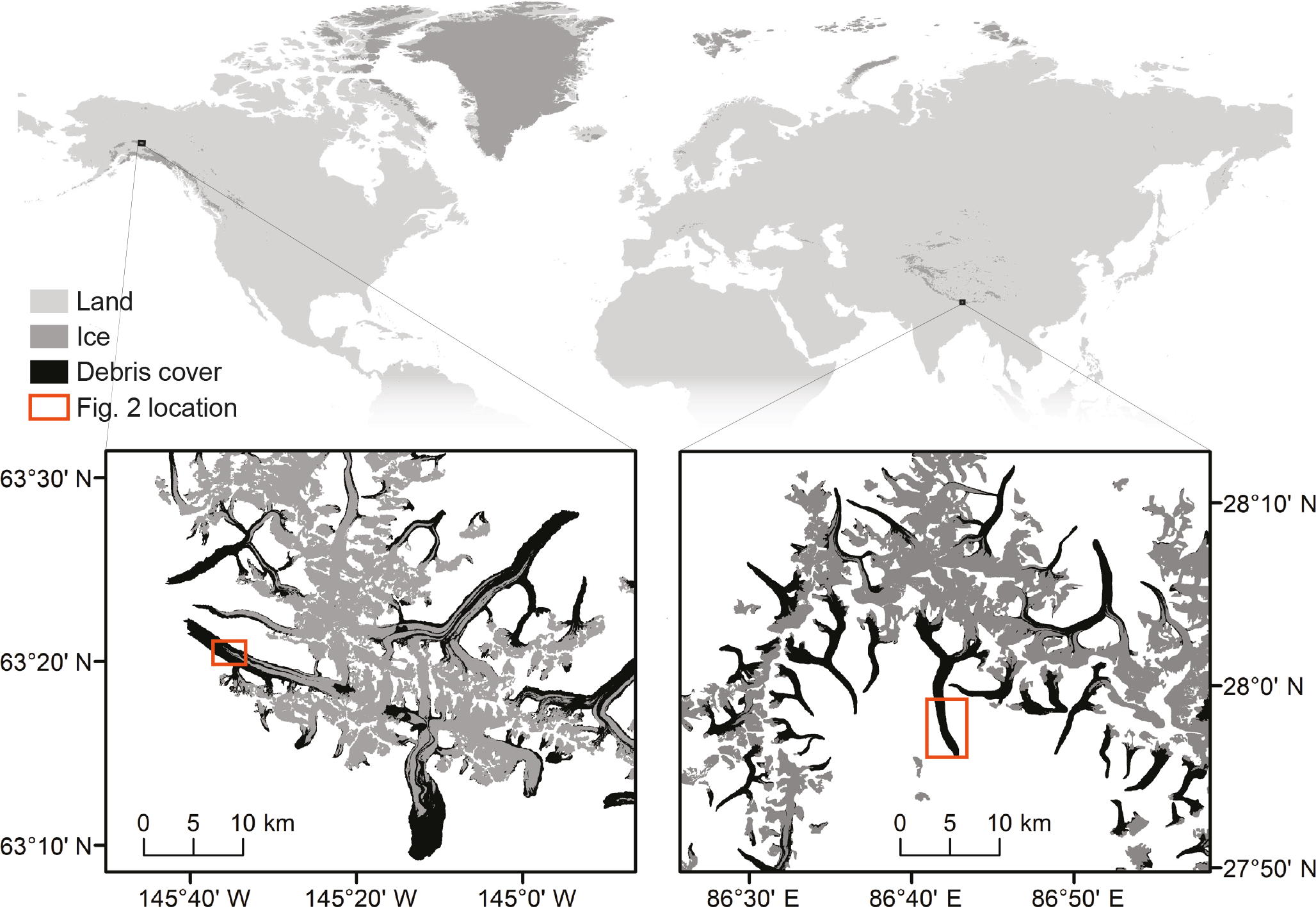
Figure 1 Location of Canwell Glacier in the eastern Alaska Range, Alaska, USA, and Ngozumpa Glacier in the Khumbu Himal, Nepal. Ice area is from Pfeffer et al. (2014) and Citterio and Ahlstrøm (2013). Scale and area shown in the two inset plots are the same.

2.2 Calibration and validation data

The parameters of this method were calibrated using manually derived ice cliff outlines based on high-resolution visible (∼ 8 cm) and thermal (80 cm) data that cover a portion of Canwell Glacier in the eastern Alaska Range, Alaska, USA. To test transferability, the same parameter set was applied to a portion of Ngozumpa Glacier in the Khumbu Himal, Nepal with an independent validation dataset previously published in Thompson et al. (2016).

2.2.1 Canwell Glacier

Canwell Glacier (Figs. 1, 2a) is a 60 km², northwest flowing glacier in the eastern Alaska Range (63^∘19.8^′ N, 145^∘32^′ W). Canwell Glacier was selected for this study because several different surface types exist in close proximity: an expansive ice cliff network in debris cover that transitions, orthogonal to flow, to bare glacier ice and a medial moraine.

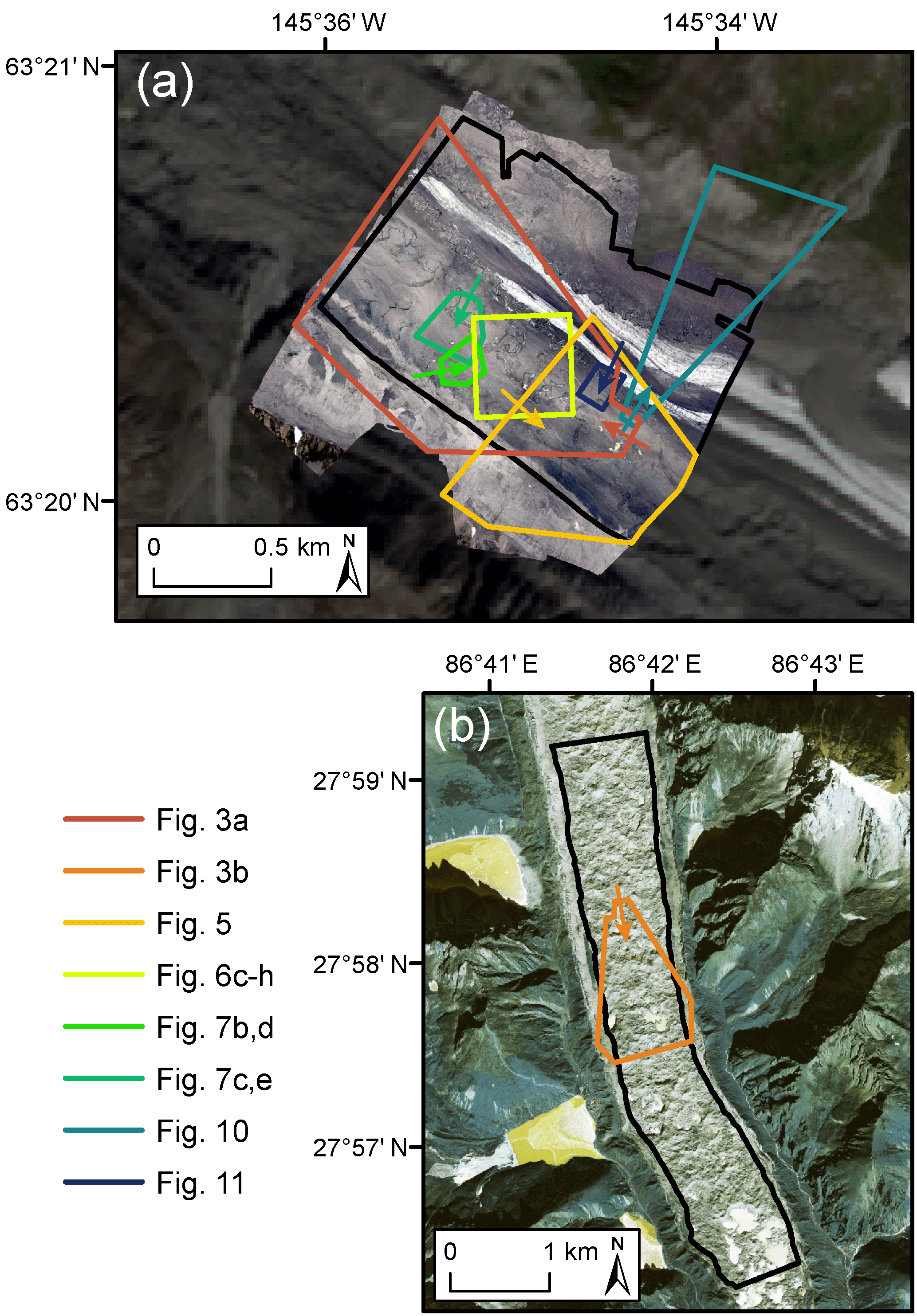
Figure 2 Study area on Canwell Glacier (a) and Ngozumpa Glacier (b). The spatial domains over which the ice cliff mapping method was applied are shown in black. The footprint of subsequent map-based figures within this paper are shown. Arrows show the look direction of figures that have an oblique orientation. The underlying imagery shown in panel (a) is the orthomosaic collected on 29 July 2016 (Sect. 2.2.1) overlain on a Landsat8 image (path/row: 67/16) acquired on 31 August 2016; and (b) the GeoEye-1 image acquired on 23 December 2012 (Sect. 2.2.2).

Figure 3 (a) Portion of Canwell Glacier, Alaska, USA, looking down glacier a distance of ∼ 1.4 km. Manually generated debris-covered area outlines and ice cliff outlines are shown in orange and red, respectively. The underlying image is an orthomosaic of visible imagery collected above Canwell Glacier on 29 July 2016, draped over a DEM derived from the same images. The inset histogram shows normalized populations of surface slopes present in the pictured debris-covered area and ice cliff area; the grey/orange region of overlap illustrates the difficulty of using surface slope alone to identify ice cliffs. Percentages give the fraction of the total area occupied by both classes (in map view). (b) Same as panel (a) but for Ngozumpa Glacier, Nepal, also looking down glacier a distance of ∼ 1.4 km. The scale in panels (a) and (b) are the same. Yellow lines are ice cliff top edges mapped by Thompson et al. (2016) which were manually expanded to ice cliff area (red) with minor additions. The underlying image and DEM are from GeoEye-1 acquired on 23 December 2012 (Sect. 2.2.2). Locations shown in Fig. 2.

On the 29 July, 2016 between 11:00 and 11:16 local time, nadir (or near-nadir) looking visible and thermal infrared images were collected from a helicopter over 1.74 km² of the Canwell Glacier capturing all of the different surface types listed above (Fig. 3a). The images were collected below a high overcast ceiling. This caused a subtle cloud effect to be captured by varying light penetration of the cloud layer, however, this also removed the likely more negative effect of shading discussed in Sect. 1. Two hundred and fifty visible spectrum images were collected with a Canon EOS 70D digital SLR camera at an altitude range of about 133–615 m above the glacier surface. Overlap between these images, in conjunction with nine ground control points, were used to generate a ∼ 8 cm resolution orthomosaic and a 1 m resolution (resampled to 5 m to match a spatial resolution more common from space borne sensors) DEM using the proprietary software Agisoft PhotoScan Professional Edition. Thirty-four (suitable for use) thermal images were collected with a FLIR T620 camera and processed using the proprietary software FLIR Tools. Emissivity was held constant at 0.95, atmospheric temperature and relative humidity where measured from the helicopter during image acquisition using a Kestrel 4000 weather meter and distance from the sensor to the glacier surface was estimated using camera locations derived by Agisoft Photoscan. The thermal images were manually georeferenced to match the orthomosaic image described above and resampled to a uniform spatial resolution of 80 cm.

A nearly cloud-free Landsat 8 image was acquired over the Canwell Glacier (path/row: 67/16) on the 31 August 2016. Debris-cover extent and glacier margins were found to be effectively static over the 33 day interval between the acquisition of the helicopter borne and Landsat 8 data.

2.2.2 Ngozumpa Glacier

Ngozumpa Glacier (Figs. 1, 2b) is a 60 km² south flowing glacier in Khumbu Himal (27^∘57^′ N, 85^∘42^′ E). Ngozumpa Glacier was selected to be used in this study for two reasons. First, it is located in a geographical region that is different from the Alaska Range with respect to latitude, longitude, continentality, climate and orogeny. These factors and others establish a setting where exposure to the sun, the overall debris cover (e.g., debris extent, clast sizes, thickness) and glacier dynamics at Ngozumpa Glacier are notably different from Canwell Glacier. Fig. 3 illustrates some differences between Canwell and Ngozumpa glaciers including rock/boulder size, ice cliff size, amount of “thin” debris cover on ice cliff faces and overall hummocky nature of the debris-covered area. The debris on Ngozumpa Glacier is thick (1–3 m towards the terminus; Nicholson, 2005) and covers the full width of the glacier continuously for nearly the entire ablation zone. The shift between the two ice cliff slope distributions shown in the two inset histograms of Fig. 3 suggest that even if overlooking overlap errors, a simple surface slope threshold deemed suitable to define ice cliffs at one location may capture a different portion of the distribution in other regions on Earth.

The second reason Ngozumpa Glacier was selected is that an automated ice cliff map can be assessed against the manually generated ice cliff map from Thompson et al. (2016), allowing the removal of some potential manual delineation bias in this study. Thompson et al. (2016) provided their GeoEye-1 orthoimage acquired on the 23 December, 2012, the corresponding stereo image derived DEM (1 m resolution, resampled to 5 m for this study) and their ice cliff map generated manually using both the orthoimage and DEM. Additionally, Thompson et al. (2016) generated and provided a mask of area where surface elevation was poorly resolved. The method Thompson et al. (2016) used to map ice cliffs was to define a line along the top edge of each ice cliff based on optical characteristics and steep surface slopes calculated from the DEM. In order to conduct a quality assessment between the top edge lines defined by Thompson et al. (2016) and the automated ice cliff polygons identified using the method presented here, the ice cliff top edges from Thompson et al. (2016) were manually adjusted to polygons incorporating the area of each ice cliff using the 23 December 2012 visible GeoEye-1 imagery. Some smaller ice cliff additions were also made.

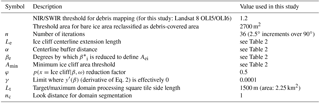
Table 1 Model parameters. Where ${{\mathit{\beta }}^{\ast }}_{\mathrm{i}}$ is the surface slope threshold that defines the base ice cliff shape (A_i) for each iteration, A_ei is the same as A_i but with a slightly lower surface slope threshold and $p(x=\mathrm{Ice}\mathrm{cliff}|\mathit{\beta },\mathit{\omega })$ is ice cliff probability given surface slope and overlap with A_cliff (Sect. 3.2.1). Look distance is the number of L_t×L_t cells the routine will look beyond and still consider as “neighboring” during segmentation of a spatial domain greater than $L_{\mathrm{t}}^{\mathrm{2}}$.

A nearly cloud-free Landsat 8 image was acquired over Ngozumpa Glacier (path/row: 140/41) on the 30 November, 2014. Because the portion of Ngozumpa Glacier considered in this study is 100 % debris-covered, a debris extent map generated with a 2-year gap does not alter the spatial domain. The glacier margin was mapped from the 23 December 2012 GeoEye-1 imagery.

3 Methods

3.1 Isolation of debris-covered area

The spatial domain is refined from total glacierized area, including bare ice and accumulation zone area, to only debris-covered glacier area. Debris-free area was identified and removed using the ratio of NIR and SWIR satellite bands (Landsat 8: OLI band 5/OLI band 6) with a user defined threshold (Paul et al., 2004) (Table 1). To prevent the removal of bare-ice pixels that are part of an ice cliff, closed shapes identified as bare ice within the debris-covered area were filled (reclassified as debris-covered area) if below a user defined threshold area (Table 1). This is possible where an ice cliff is debris-free and big enough to cause one or more satellite image pixels to fall below the NIR/SWIR ratio threshold.

3.2 Ice cliff identification

3.2.1 Iterative ice cliff detection

Within debris-covered area, surface slope, β, is calculated as the maximum elevation difference for each DEM pixel value relative to its eight neighbor values. A threshold slope value, β_i, isolates steeper area from which statistics and further threshold values are derived. This area, and all subsequent areas derived in the mapping method, are simplified as a shape in two dimensions (2-D). Only final results of the mapping method are converted to 3-D surfaces (method described in Sect. 3.4 and referred to synonymously as “true surface area” and “area considering slope”). The method is run iteratively, varying β_i over the full range of possible surface slopes (neglecting over-vertical surfaces), from 0 to 90^∘ in n number of iterations (i).

For each i, two areas are defined that will, together, define area with a high likelihood of being an ice cliff: (1) an initial ice cliff area (A_i) from which statistics are computed, further geometries are derived and the base shape of the final ice cliff area is defined; and (2) A_ei, an area slightly more encompassing than A_i from which lengthwise ends of the final ice cliff geometries are extracted (subscript “e” for “end”).

A_i is defined as area$(\mathit{\beta }>{{\mathit{\beta }}^{\ast }}_{\mathrm{i}})$ where ${{\mathit{\beta }}^{\ast }}_{\mathrm{i}}=\mathrm{mean}(\mathit{\beta }>{\mathit{\beta }}_{\mathrm{i}})$ (Fig. 4a). Using ${{\mathit{\beta }}^{\ast }}_{\mathrm{i}}$ rather than simply β_i speeds up computation by discarding the case where ice cliffs occupy an overwhelming percentage (≫ 50 %) of the debris-covered area. If ice cliffs did occupy one half or more of a debris-covered area (in map view), its classification as a debris-covered portion of a glacier could be questioned.

Figure 4 Method used to define ice cliff area, $A_{{\mathrm{cliff}}_{\mathrm{i}}}$ for each iteration, i, and a final, optimized iteration, subscript opt. Surface slope threshold β_i is applied over the range 0–90^∘ from which the subsequent quantities shown in steps a–d are calculated. Quantities in bold font are fixed scalar model parameters that do not vary over the iterative process. Panel (a) shows how the area A_i is defined by ${{\mathit{\beta }}^{\ast }}_{\mathrm{i}}$, the mean surface slope of values constrained by β_i. A procedure using a Voronoi partition defines a centerline within A_i. Panel (b) shows this centerline extended by a distance of L_e, and transformed into an area, B_ei, by an outward buffer distance, α, applied in all (x,y) directions. Panel (c) shows the definition of A_ei, an area defined by a surface slope threshold lower than ${{\mathit{\beta }}^{\ast }}_{\mathrm{i}}$, where ${{\mathit{\beta }}^{\ast }}_{\mathrm{i}}$ is reduced by β_e. The intersection of A_ei and the buffer area, B_ei, define C_ei. C_ei allows allow for the identification of ice cliff end area that has a surface slope below ${{\mathit{\beta }}^{\ast }}_{\mathrm{i}}$ and above A_ei while rejecting area that falls within the same surface slope interval but is not located at the ends of an ice cliff. The intersection of A_i and C_ei, with areas below a threshold, A_min, removed, defines the final ice cliff area, $A_{{\mathrm{cliff}}_{\mathrm{i}}}$, for that i (d).

Ice cliff centerlines are computed by creating a Voronoi cell for each vertex in the outline of A_i converted to a dense set of vertices. The bounding edges of each Voronoi cell is removed except for the edge in the center of a shape in A_i. A point removal line simplification is applied to smooth extraneous bends, particularly at centerline ends. The centerline ends are then extended by a user defined distance, L_e (Fig. 4b), with the topological restriction that centerline extensions can intersect, but not cross one another. The extended centerlines are then transformed to an area, B_ei, by a buffer distance, α, applied outward in all directions (Fig. 4b). C_ei is the intersection of B_ei and A_ei, where A_ei is area with a surface slope greater than ${{\mathit{\beta }}^{\ast }}_{\mathrm{i}}$ relaxed by a user defined factor, β_e (Fig. 4c). C_ei is intended to identify area that is part of an ice cliff but expressed by surface slopes less than ${{\mathit{\beta }}^{\ast }}_{\mathrm{i}}$ due, possibly, to narrowing ice cliff ends where DEM data and subsequent surface slope calculations saturate a true, steep surface slope signal. Area with a high likelihood of being an ice cliff, $A_{{\mathrm{cliff}}_{\mathrm{i}}}$, is defined as the union of C_ei and A_i where a user defined minimum shape area threshold, A_min is exceeded (Fig. 4d).

$A_{{\mathrm{cliff}}_{\mathrm{i}}}$ is the definitive ice cliff area used for the error analysis in Sect. 3.5 after optimization described in Sect. 3.2.2, but for some applications of this method, a distributed probability map might be a more useful product. With β_i as a lower limit and β_u, where ${\mathit{\beta }}_{\mathrm{u}}={{\mathit{\beta }}^{\ast }}_{\mathrm{i}}+$ SD (β>β_i), as an upper limit, the probability that a pixel, x, is part of an ice cliff can be estimated as follows:

$$\begin{array}{ll}{\displaystyle }& {\displaystyle }p(x=\mathrm{Ice}\mathrm{cliff}|\mathit{\beta },\mathit{\omega })=\\ \text{(1)}& {\displaystyle }& {\displaystyle }\left\{\begin{array}{ll}\mathrm{0},& \mathit{\beta }<{\mathit{\beta }}_{\mathrm{i}},\mathit{\omega }=\mathit{\{}\mathrm{1},\mathrm{0}\mathit{\}}\\ \frac{\mathit{\beta }+{\mathit{\beta }}_{\mathrm{i}}}{{\mathit{\beta }}_{\mathrm{u}}-{\mathit{\beta }}_{\mathrm{i}}},& {\mathit{\beta }}_{\mathrm{i}}\le \mathit{\beta }\le {\mathit{\beta }}_{\mathrm{u}},\mathit{\omega }=\mathrm{1}\\ \frac{\mathit{\phi }(\mathit{\beta }+{\mathit{\beta }}_{\mathrm{i}})}{{\mathit{\beta }}_{\mathrm{u}}-{\mathit{\beta }}_{\mathrm{i}}},& {\mathit{\beta }}_{\mathrm{i}}\le \mathit{\beta }\le {\mathit{\beta }}_{\mathrm{u}},\mathit{\omega }=\mathrm{0}\\ \mathit{\phi },& \mathit{\beta }>{\mathit{\beta }}_{\mathrm{u}},\mathit{\omega }=\mathrm{0}\\ \mathrm{1},& \mathit{\beta }>{\mathit{\beta }}_{\mathrm{u}},\mathit{\omega }=\mathrm{1}\end{array}\right..\end{array}$$

From Eq. (1), ice cliff probability is assigned given surface slope, β, and ω, where ω is a binary classification {1,0} for pixels falling within $A_{{\mathrm{cliff}}_{\mathrm{i}}}$, one, and outside $A_{{\mathrm{cliff}}_{\mathrm{i}}}$, zero. For pixels where ω=0, ice cliff likelihood is reduced by a user defined factor, φ. φ=0 implies the iterative process will have zero error, φ=1 discards the entire iterative process and φ=0.5 (for example) means that a surface slope greater than β_u but not bound by a high likelihood ice cliff shape ($A_{{\mathrm{cliff}}_{\mathrm{i}}}$) will be assigned a $p(x=\mathrm{Ice}\mathrm{cliff}|\mathit{\beta },\mathit{\omega })$ value of 0.5. With this use of φ=0.5 as a reduction factor, area iteratively identified as ice cliff will be assigned a $p(x=\mathrm{Ice}\mathrm{cliff}|\mathit{\beta },\mathit{\omega })$ that is a factor of 0.5 greater than any other area but no steep surface slope will be completely rejected as having $p(x=\mathrm{Ice}\mathrm{cliff}|\mathit{\beta },\mathit{\omega })=\mathrm{0}$.

The result of this iterative process is 90∕n gridded ice cliff probability maps and vector ice cliff shapes ($A_{{\mathrm{cliff}}_{\mathrm{i}}}$) for the entire spatial domain.

3.2.2 Heuristic selection of β_opt: a best β_i

The 90∕n ice cliff probability maps are constrained by two conditions: (1) the spatial domain is unrealistically dense with ice cliff, and (2) there is zero ice cliff area. Using the resulting ice cliff area ($A_{{\mathrm{cliff}}_{\mathrm{i}}}$), ice cliff fraction, y_i, is calculated as $A_{{\mathrm{cliff}}_{\mathrm{i}}}/\mathrm{area}\left(\mathrm{spatial}\mathrm{domain}\right)$. To derive a continuous, functional form of ice cliff fraction, the equation

$$\begin{array}{}\text{(2)}& y\left(\mathit{\beta }\right)=a\exp \left(-{\left({\displaystyle \frac{\mathit{\beta }-b}{c}}\right)}^{\mathrm{2}}\right)\end{array}$$

is fit to y_i and β_i using non-linear least squares where a, b and c are fitting parameters. The curve expresses unrealistically high y(β) with low values of β because the threshold slope for ice cliff classification is well below slopes from surface roughness/undulations common for a debris-covered portion of a glacier. If there are ice cliffs within the spatial domain, the increase in β towards 90^∘ causes the threshold to become too stringent, excluding even true ice cliff area. Steep ice cliff faces (and possibly erroneous DEM data) will cause iterations to run through high values of β with minor reductions in y(β) causing the slope of y(β), y^′(β), to gradually approach 0 as β approaches 90^∘. If there are no ice cliffs within the spatial domain, the iterative process will end as soon as $A_{{\mathrm{cliff}}_{\mathrm{i}}}=\mathrm{0}$, which will likely occur at a lower β relative to a spatial domain with ice cliffs because debris cover can only be maintained on a subset distribution of surface slopes (see inset histograms in Fig. 3). This truncation is likely the key distinction of areas with no ice cliffs relative to ice cliff abundant domains (see Sect. 5.2). If there are ice cliffs within the spatial domain, some value of β_i will optimize a match with the true ice cliff fraction. The method uses a heuristic approach to select this β_i, termed β_opt, which might provide the most accurate final A_cliff and coupled $p(x=\mathrm{Ice}\mathrm{cliff}|\mathit{\beta },\mathit{\omega })$ map.

Where β is low and y(β) is unrealistically high, all ice cliffs will likely be included (high true positive rate (defined in Sect. 3.5)) yet will be accompanied by a large amount of non-ice-cliff area (low precision (defined in Sect. 3.5)). Conversely, as β approaches 90^∘, or max(β) if $max\left(\mathit{\beta }\right)<\mathrm{90}$^∘, the small areas within y(β) will very likely be ice cliff area (high precision), but widely under-resolve the true ice cliff area (low true positive rate). In the absence of validation data to explicitly optimize true positive rate and precision, the “elbow” of the curve as y(β) shifts from a steep slope, high y^′(β), to y^′(β) approaching 0, is hypothesized to correspond to the optimized maximum of both true positive rate and precision (Fig. 6). The hypothesis is that as β_i increases and less sloped debris-covered area (e.g., from strain and differential melt) is included as mapped ice cliff, true ice cliffs will begin to comprise the majority of the mapped ice cliff fraction (y_i). We hypothesize this to have a stabilizing effect (ice cliffs are a small, consistently steep area), lowering the rate of loss of mapped ice cliff area and slope of the curve as β_i continues towards 90^∘. We hypothesize that this so-called “elbow” point will thereby identify a β_opt that reflects a surface slope characteristic common to the small spatial domain the method is applied to, but possibly unique to a geographical region or latitude. This point, (β_opt,y_opt) is defined as

$$\begin{array}{}\text{(3)}& ({\mathit{\beta }}_{\mathrm{opt}},y_{\mathrm{opt}})=(\mathit{\beta },y(\mathit{\beta }\left)\right)\mathrm{where}(\mathit{\beta },y(\mathit{\beta }\left)\right)\cap max\left(d\right),\end{array}$$

where

$$\begin{array}{ll}{\displaystyle }d& {\displaystyle }=\mathrm{distance}(P_{\mathrm{1}},P_{\mathrm{2}},(\mathit{\beta },y\left(\mathit{\beta }\right)\left)\right)\\ \text{(4)}& {\displaystyle }& {\displaystyle }={\displaystyle \frac{\left|(y_{\mathrm{2}}-y_{\mathrm{1}}){\mathit{\beta }}_{\mathrm{i}}-({\mathit{\beta }}_{\mathrm{2}}-{\mathit{\beta }}_{\mathrm{1}})y+{\mathit{\beta }}_{\mathrm{2}}{y}_{\mathrm{1}}-y_{\mathrm{2}}{\mathit{\beta }}_{\mathrm{1}}\right|}{\sqrt{(y_{\mathrm{2}}-y_{\mathrm{1}}{)}^{\mathrm{2}}+({\mathit{\beta }}_{\mathrm{2}}-{\mathit{\beta }}_{\mathrm{1}}{)}^{\mathrm{2}}}}}.\end{array}$$

d is the orthogonal distance from a line defined by points P₁ and P₂ to the function y(β) (Eq. 2), where

$$\begin{array}{ll}{\displaystyle }& {\displaystyle }{P}_{\mathrm{1}}=({\mathit{\beta }}_{\mathrm{1}},y_{\mathrm{1}})\\ {\displaystyle }& {\displaystyle }{\mathit{\beta }}_{\mathrm{1}}=\mathit{\beta }\mathrm{where}{y}^{\prime }\left(\mathit{\beta }\right)=\mathit{\gamma }\\ \text{(5)}& {\displaystyle }& {\displaystyle }{y}_{\mathrm{1}}=y\left({\mathit{\beta }}_{\mathrm{1}}\right)\end{array}$$

and

$$\begin{array}{ll}{\displaystyle }& {\displaystyle }{P}_{\mathrm{2}}=({\mathit{\beta }}_{\mathrm{2}},y_{\mathrm{2}})\\ {\displaystyle }& {\displaystyle }{\mathit{\beta }}_{\mathrm{2}}=\mathit{\beta }\mathrm{where}y\left(\mathit{\beta }\right)=max\left(y\right(\mathit{\beta }\left)\right)\\ \text{(6)}& {\displaystyle }& {\displaystyle }{y}_{\mathrm{2}}=y\left({\mathit{\beta }}_{\mathrm{2}}\right).\end{array}$$

γ is an input parameter with a near zero value (Table 1) defining the limit when y^′(β) is effectively zero. Since the function asymptotically approaches zero, without γ, β₁ would always be 90^∘ and this geometric approach would likely fail to identify the so called “elbow” of the curve. Additionally, DEM errors can sometimes have vertical or near vertical slopes (e.g., a raised artifact). These errors will be identified as ice cliff area but will not impede the calculation of (β_opt,y_opt) because very steep area causes a vertical translation of the function y(β), thus not affecting y^′(β). An alternative approach could use higher order derivatives to identify (β_opt,y_opt) thus eliminating the parameter γ, but this approach might be unreliable due to numerical instability.

A final application of the model where β_i=β_opt produces a final automated ice cliff probability map. If visual inspection suggests large errors, all of the ice cliff probability maps and resulting ice cliff area shapefiles generated from the earlier set of iterations are retained and can be manually assessed to establish if a more adequate β_i value should be considered optimal. Future applications of this method that produce large errors might indicate that a fixed γ value is not suitable for all regions or that the surface slope distributions of debris-covered and ice cliff area have too much overlap to use surface slope alone as a deterministic attribute.

3.3 Domain segmentation for large areas

Using this method over large spatial domains might be computationally demanding on typical desktop or laptop computers. To address this, a precursory function segments large domains (considering only debris-covered area) into less computationally taxing tiles. Because the ice cliff mapping depends on statistics calculated across the entire area considered, it is critical that segments are large enough so that meaningful statistics can be computed. A target/maximum spatial domain is defined by the user as the length of an edge of a square, L_t. If the debris-covered area of interest is below $L_{\mathrm{t}}^{\mathrm{2}}$, no segmentation will be applied. If the debris-covered area is greater than $L_{\mathrm{t}}^{\mathrm{2}}$, the debris-covered area is subdivided by a square grid with side length L_t. The function finds the area of debris cover occupying each grid cell and attempts to merge neighboring cells one at a time until their fractional debris-covered area sum to one. A look distance factor in number of L_t×L_t cells, n_c, controls if and how far the method will look beyond empty space or cells where an unsuccessful match (summed fraction > 1) occurred and still be considered as “neighboring” cells. When a cell or set of previously merged cells have (1) exhausted the set of possible neighboring cells within the look distance, and (2) have all returned a summed debris cover fraction greater than one, the cell or set of cells are defined as a closed tile that will become an input spatial domain to the iterative and heuristic optimization scheme. The method automatically identifies and individually processes each tile and a final merged product of both gridded $p(x=\mathrm{Ice}\mathrm{cliff}|\mathit{\beta },\mathit{\omega })$ and a vector shapefile corresponding A_cliff are generated.

3.4 Derivation of a calibration dataset for Canwell Glacier

To calibrate a method that automatically maps ice cliff area, a sufficiently accurate “truth” dataset is needed. For this study, ice cliff outlines generated from the high-resolution visible and thermal data described in Sect. 2.2.1 were considered to be true. Elevation data described in Sect. 2.2.1 were not explicitly used to digitize from but were used in a 3-D viewer with draped visible and thermal layers to assess generated ice cliff outline quality. Area that was clearly ice cliff in visible and thermal data but not apparent in elevation data (possibly due to errors in the DEM) was still mapped as ice cliff area. Given the ambiguities described in Sect. 1 regarding “thin” debris cover, ice cliffs were liberally outlined, including, for example, cliffs that were nearly 100 % covered by debris, yet had a unique thermal signature relative to the surrounding debris cover indicating thinner debris. No minimum size was considered, thus ice cliffs below the resolution of the method input data are penalized in quality assessment metrics, if missed. While we made an effort to manually map ice cliffs based on consistent criteria, there is subjective interpretation within this “truth” dataset. We did not quantify the uncertainty associated with this subjectivity.

True surface area (area considering slope, as opposed to map-view surface area) was calculated to present final results (Sects. 4 and 5.3) by multiplying DEM pixel area by a factor correcting for constant-sloped terrain (cos(β)⁻¹, the secant of slope angle) for each pixel and finding the sum of slope corrected area for all ice cliff pixels or pixels within the entire spatial domain.

3.5 Statistical measures of performance

A suite of statistical measures of performance are needed to isolate and illustrate performance trade-offs and rank success between parameter sets and alternative, less complex methods. All performance metrics are calculated using the final output ice cliff area A_cliff rather than distributed $p(x=\mathrm{Ice}\mathrm{cliff}|\mathit{\beta },\mathit{\omega })$. True positive (TP) is defined as area where the ice cliff mapping technique output intersects true ice cliff area. True negative (TN) is defined as area where the method correctly identified non-ice-cliff area (debris-cover area). False positive (FP) and false negative (FN) are defined as area identified as ice cliff that is not in the “true” dataset and ice cliff area present in the “true” dataset but absent in the automated output, respectively. Using these quantities, the following common metrics (Fawcett, 2006) are defined:

$$\begin{array}{}\text{(7)}& {\displaystyle }& {\displaystyle }\mathit{\text{true positive rate}}={\displaystyle \frac{\mathrm{TP}}{\mathrm{TP}+\mathrm{FN}}}\text{(8)}& {\displaystyle }& {\displaystyle }\mathit{\text{precision}}={\displaystyle \frac{\mathrm{TP}}{\mathrm{TP}+\mathrm{FP}}}\text{(9)}& {\displaystyle }& {\displaystyle }\mathit{\text{accuracy}}={\displaystyle \frac{\mathrm{TP}+\mathrm{TN}}{\mathrm{TP}+\mathrm{FP}+\mathrm{FN}+\mathrm{TN}}}.\end{array}$$

True positive rate (also called recall) is the ratio of successful classification over total true ice cliff area and precision measures the probability that area identified as ice cliff is in fact ice cliff. Ideally, these metrics should be equal to each other and, if the cliff mapping is perfect, both equal one. Accuracy is the proportion of true results, but because ice cliffs will most often occupy a small fraction of a debris-covered area and accuracy accounts for TN as well as TP, it becomes a less informative metric. For example, if 1 % of a debris-covered portion of a glacier is ice cliff, not mapping ice cliffs at all will yield an ice cliff mapping accuracy of 99 %. We therefore introduce two additional metrics, outside of the standard suite of statistical measures of performance, that are independent of TN and thus help evaluate ice cliff mapping success:

$$\begin{array}{}\text{(10)}& {\displaystyle }& {\displaystyle }\mathit{\text{error distribution}}={\displaystyle \frac{\mathrm{FP}}{\mathrm{FN}}}\text{(11)}& {\displaystyle }& {\displaystyle }\mathit{\text{error magnitude}}={\displaystyle \frac{\mathrm{FP}+\mathrm{FN}}{\mathrm{TP}+\mathrm{FN}}}.\end{array}$$

Error distribution provides a measure of balance between FP and FN errors. An error distribution  greater than one means there is more debris-covered area mapped erroneously as ice cliff than ice cliff area erroneously mapped as debris-covered and vice versa. Ideally, error distribution is one. Error magnitude is a ratio of the total erroneously mapped area, both FP and FN, over the manual “true” ice cliff area (which is equal to the sum of TP and FN). If error magnitude is zero ice cliffs are perfectly mapped, if error magnitude is, for example, two, then error is a factor of two greater in spatial extent than the true ice cliff area.

3.6 Calibration

The method presented here requires five key input parameters to map ice cliffs: L_e, α, β_e, A_min and γ (Table 1, described in Sect. 3.2.1, bold font quantities in Fig. 4). A matrix of different parameter sets were tested using Canwell Glacier data. The success of each parameter set was quantified against the manually generated ice cliff outlines described in Sect. 3.4 using the statistical measures of performance derived in Sect. 3.5.

3.7 Quantification of “thin” debris cover on ice cliffs

As described in Sect. 1, ice cliffs can be considerably covered by rock fragments. The automated method presented here uses elevation data alone and therefore depends on the assumption that steep terrain within a debris cover is ice cliff. Because the validation data described in Sect. 3.4 is in part visible data, assessment of “thin” debris cover on ice cliffs can be made and used to further interpret automated ice cliff mapping results. The optical orthomosaic was converted to greyscale and a pixel value threshold was selected manually that discriminated between debris-free and debris-covered area. We did not quantify the sensitivity of this threshold parameter and relied on visual assessment (e.g., comparing panels b and c to panels d and e in Fig. 7) to determine a single value that minimized errors (e.g., due to varying lithology) and maximized success. This process is similar to the satellite data based method described in Sect. 3.1 to identify debris-covered area, but without a band ratio correction and at a much higher spatial resolution of ∼ 8 cm. The results provide an estimate of the distribution and fraction of debris cover on ice cliffs (Fig. 7).

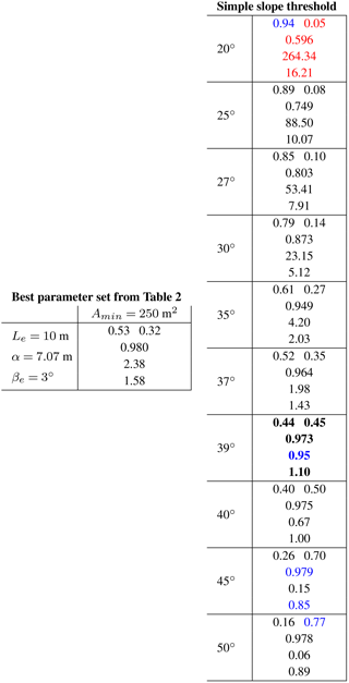
Table 2 Model parameter calibration at Canwell Glacier using statistical measures of performance derived in Sect. 3.5. True positive rate is abbreviated here as TP rate. A well performing parameter set will have values of true positive rate and precision that are as close to one as possible and balanced. Variation of A_min was tested at 0, 5 and 10 DEM pixels; L_e at 2× and 4× pixel length; and α at (pixel length × $\sqrt{\mathrm{2}}$) ∕ 2 and pixel length × $\sqrt{\mathrm{2}}$. Values in bold font are the highest ranking parameter sets and values in blue and red are the best and worst values, respectively, for all boxes in the table.

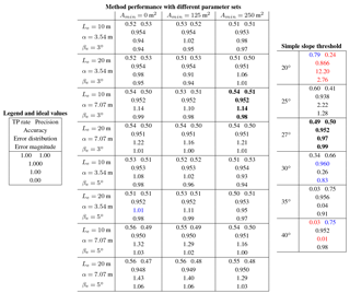
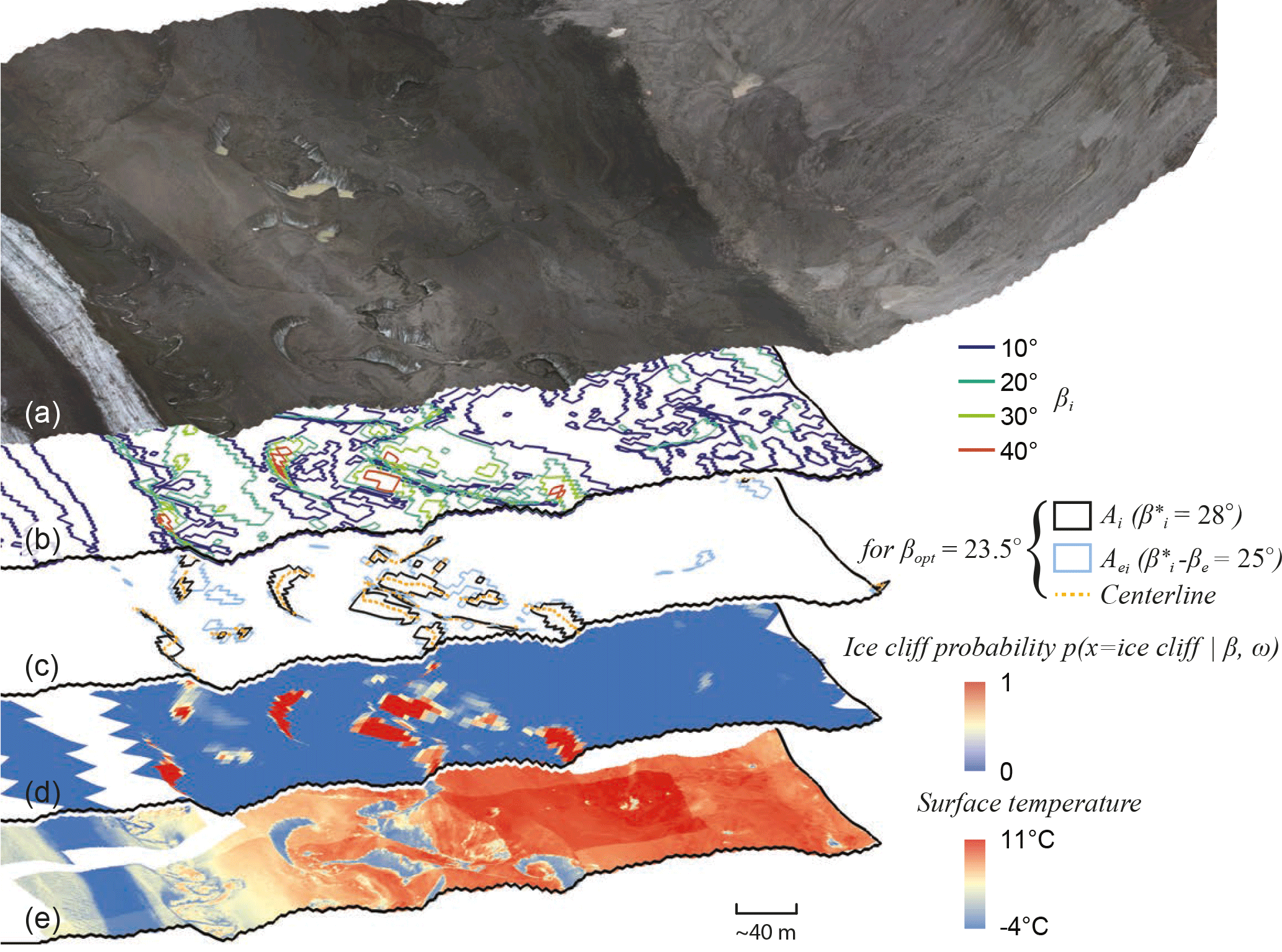
Figure 5 (a) Orthomosaic of visible imagery collected above Canwell Glacier on 29 July 2016, draped over a DEM derived from the same images. Panel (b) shows the area enclosed for select surface slope thresholds, β_i, during the iterative process. Panel (c) shows intermediate quantities calculated during the final iteration using β_opt, the optimized β_i. The area enclosed by A_ei and the ice cliff centerlines are used to add low angle area at the ends of ice cliffs to the area A_i, the main ice cliff shape defined from ${{\mathit{\beta }}^{\ast }}_{\mathrm{i}}$. Panel (d) shows the final distributed map of $p(x=\mathrm{Ice}\mathrm{cliff}|\mathit{\beta },\mathit{\omega })$, the computed probability that a given pixel will fall within true ice cliff area, assigned as a function of surface slope, β, and ω, the overlap with the final vector ice cliff shape, A_cliff, generated from the quantities shown in panel (c). (e) Orthomosaic of thermal imagery collected on 29 July 2016, draped over the same DEM from panel (a). Location shown in Fig. 2.

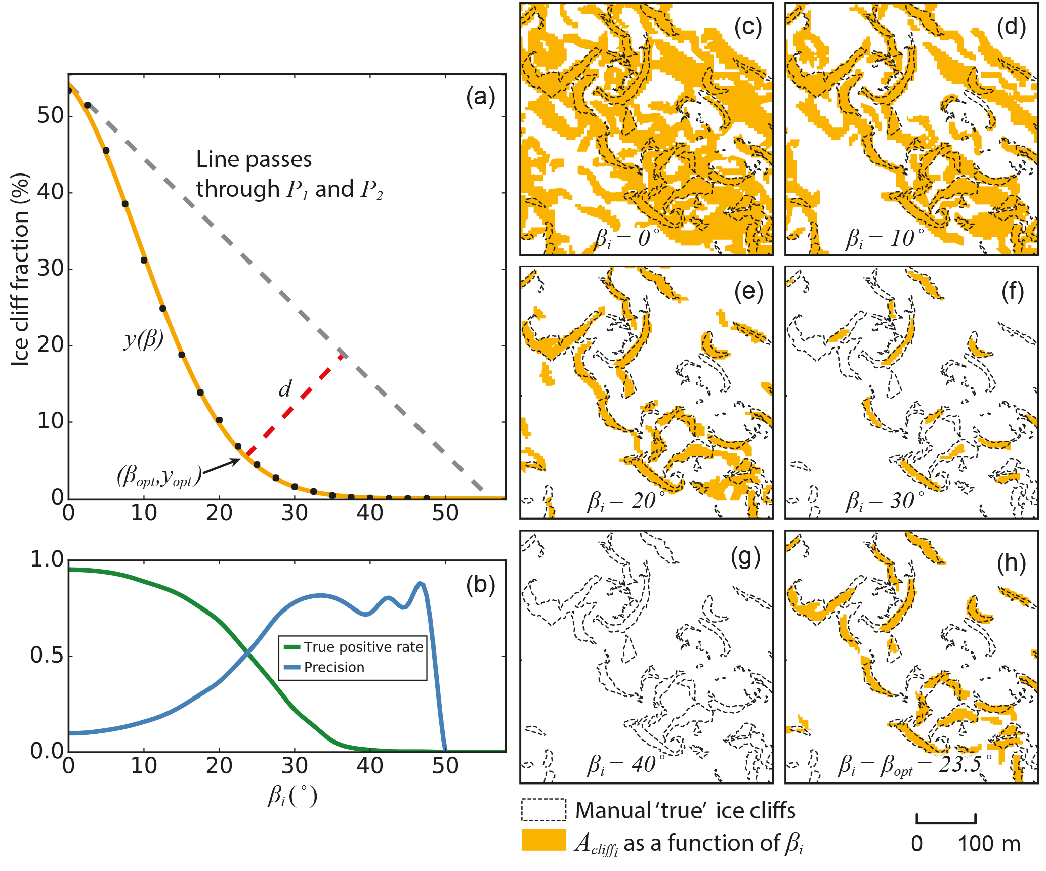
Figure 6 Panel (a) shows the heuristic method for selecting β_opt. Black dots are computed values of the fraction of area ice cliffs occupy within the spatial domain for each β_i in n number of iterations (i). The orange curve, y(β), is a function fit to these points (Eq. 2). β_opt is found by finding the longest distance, d, between y(β) and a line passing through points P₁ and P₂ (Eqs. 5 and 6). β_opt is hypothesized to be coincident with the intersection of true positive rate and precision, the optimized, best possible balance of errors. (b) True positive rate and precision (derived in Sect. 3.5) comparing method results for each β_i to “true” ice cliff area mapped from high-resolution optical and thermal data (Sect. 2.2.1). Panels (c–g) show the respective ice cliff maps ($A_{{\mathrm{cliff}}_{\mathrm{i}}}$) for x axis ticks in panels (a) and (b) up to β_i=40^∘, with “true” ice cliff area overlain for reference. Panel (h) shows the iterative method run a final time where β_i=β_opt and defines the automatically selected best ice cliff map. Location of panels (c–h) shown in Fig. 2.

Figure 7 (a) Each “true” manually mapped ice cliff on Canwell Glacier is shown as a circle sized proportionally to map-view surface area and plotted against the mean ice cliff surface slope and the percentage of “thin” debris cover on the ice cliff face. The color scale shows the true positive rate from the automated ice cliff mapping method derived for each ice cliff. FP ice cliffs, defined as isolated shapes that are solely FP area and do not share a boundary with a “true” ice cliff, are colored grey and abbreviated as FP on the axis label. Two ice cliffs (C1 and C2) are shown to illustrate how “thin” debris cover was mapped and provide context to the data presented in panel (a). Panels (b) and (c) are oblique views of the 29 July 2016 Canwell Glacier orthomosaic with manually generated ice cliff outlines shown in orange. Panels (d) and (e) are the same views with the orthomosaic processed to identify only debris cover on ice cliff faces. C1 is nearly 100 % debris-covered which could draw its classification as an ice cliff into question. C2 is one of the more “clean” ice cliffs within the Canwell Glacier study area but is still covered by a non-trivial amount, > 50 %, of debris. C1 shows linear englacial debris bands that contribute to the ice cliff face debris accumulation. Location shown in Fig. 2.

4 Results

4.1 Canwell Glacier

The manually generated, “true” ice cliff dataset shows 4.9 % of the 1.74 km² Canwell Glacier study area is ice cliff in map view (not considering slope). Ice cliff map-view area (84 630 m²) under-represents true ice cliff surface area (104 920 m², considering slope) by 19 %. Considering the true surface area of the Canwell Glacier study area, map view under-represents true surface area (1.86 km²) by 6 %. Considering the true surface area of both ice cliffs and the Canwell Glacier study area, the fraction of ice cliff area is 5.7 %.

Running the automated method 24 times with the same input data while varying the input parameters over a series of different parameter sets (Table 2) produced two main results. The varying parameter set results (1) suggest that the method is stable and robust because no parameter set produced exceptionally poor results (e.g., computed error magnitude across all parameters sets in Table 2 fall within a range of 0.94 to 1.06); and (2) allow the selection of a “best” parameter set, selected with an emphasis on high and equal values of true positive rate and precision: L_e = 10 m, α = 3.54 m, β_e = 3^∘ and A_min = 250 m² (Fig. 5). γ is excluded from Table 2 because after testing different values of γ, a value of 0.0001 consistently returned results where true positive rate and precision are close to equal. Calibration results in Table 2 are shown alongside the same statistical measures of performance applied to a range of simple surface slope thresholds used to identify ice cliffs. This comparison shows that a carefully selected slope threshold can provide an ice cliff map comparable in statistical measure to the more complex method presented here. However, simple slope threshold results are shown to be sensitive with respect to the slope value used and would require additional data, similar in quality to those described in Sect. 3.4, to validate the threshold selection and subsequent results.

Using the parameter set [L_e = 10 m, α = 3.54 m, β_e = 3^∘, A_min = 250 m² and γ = 0.0001] as input, Fig. 6 shows the heuristic approach for selecting β_opt. β_opt is calibrated so that there is close coincidence between β_opt and β where true positive rate and precision intersect (Fig. 6). Error magnitude deviated only slightly from a value of one in all of the parameter set tests. This indicates the best results of this method are incurring errors equal in area to the true area of ice cliffs. This is a non-trivial error but likely an unavoidable trade-off for a method designed for wide scales and modest data input. It is important to note that comparing only percent ice cliff area values between manually mapped ice cliffs (4.9 %), and modeled (5.3 %) would give a misleading perception of very low error, 0.4 %. The true error is closer to 5 % (1 − accuracy) if considering the entire domain or higher if considering only ice cliff area error (true positive rate and precision). For most tests, errors are fairly distributed between FP and FNs and shown by error distribution having a proximity to one. As described in Sect. 3.5, accuracy is a poor indicator of success mapping a feature that occupies a small fraction of a total area, favoring a setting of higher precision over true positive rate, but it is the only metric used in this study that rewards TN area and quantifies overall performance.

Results using the best parameter set for Canwell Glacier have an accuracy of 0.952, where FP and FN errors are close to evenly distributed with an error distribution of 1.14 and an error magnitude of 0.98, which is slightly below the mean for all tested parameter sets (0.99). True positive rate and accuracy are higher (0.54 and 0.51, respectively) than those achieved by the best simple slope threshold, 27^∘ (0.49 and 0.50, respectively). These results suggest that the method presented here can achieve results that are slightly more accurate than the best simple slope threshold and is more robust: sensitivity to changing parameters is low while different simple slope threshold values produce wider variance in statistical measures of performance (Table 2) and are thus more sensitive.

Mapping success in the context of ice cliff characteristics

Figure 7 shows mean surface slope, map-view surface area and the percentage of “thin” debris covering every manually mapped ice cliff. These characteristics are shown in the context of true positive rate (Eq. 7) now calculated for every ice cliff (true positive rate mentioned in all instances prior was calculated for all ice cliffs together), and FP ice cliffs, which we define as isolated shapes that are solely FP area and do not share a boundary with a shape in the manually mapped “true” ice cliff area. The figure shows a clear true positive rate dependence on slope, illustrating the limitations of this method to detect ice cliffs where steep surface slopes were not sufficiently resolved in the data. The figure shows that, in this portion of Canwell Glacier, most of the “cleanest” ice cliffs are still covered by a non-trivial (> 50 %) amount of debris. The percentage of “thin” debris cover on ice cliff faces appears continuous above 50 %, such that there is no clear boundary in the data that could define what is and is not an ice cliff if the percentage of “thin” debris cover was the main deterministic variable.

Table 3 Statistical measures of performance for Ngozumpa Glacier. The arrangement of metrics in each box, bold font and coloration are the same as in Table 2.

4.2 Ngozumpa Glacier

Applying the best parameter set found for Canwell Glacier to the lower ablation zone of Ngozumpa Glacier (4.8 km²) produced a decrease in performance (Table 3). For example, true positive rate, precision and error magnitude for Canwell Glacier are 0.54, 0.51 and 0.98, respectively, and 0.53 (−1 %), 0.32 (−19 %) and 1.58 (+0.6), respectively, for Ngozumpa Glacier. The imbalance between true positive rate and precision indicates the automatically selected β_opt does not coincide with the ideal β_i where true positive rate and precision are optimized. However, in the context of the simple slope threshold results shown in Table 3, the best possible threshold is 39^∘ and the statistical measures of performance from the automated method are closest to a simple slope threshold of 37^∘. This suggests that the automated method missed selecting optimum threshold(s) by about 2^∘. Considering that not a single alteration was made to the method and input parameter values used for Canwell Glacier, the method mitigated the many physical differences between Canwell and Ngozumpa glaciers (described in Sect. 2.2.2 and shown in Fig. 3) as well as different DEM generation methods (satellite based rather than airborne structure from motion). This ability to accommodate different physical characteristics enables the method to outperform a simple slope threshold found at one location, e.g., at Canwell Glacier, and assume that it is transferable to other places on Earth, e.g., Ngozumpa Glacier (Tables 2 and 3). The debris-covered area considered on Ngozumpa Glacier was broken into three processing tiles where β_opt found for each tile was 30.8, 32.5, and 33.5^∘, while β_opt for Canwell Glacier was 23.5^∘. The ∼ 10^∘ difference between β_opt for both glaciers is significant but appropriate for each location as shown in Fig. 3 or observed by comparing the statistical measures of performance for the range of simple slope threshold values shown in the far right column of Tables 2 and 3. Taking the best simple slope threshold of 27^∘ found for Canwell Glacier and applying it to Ngozumpa Glacier would result in an ice cliff map with a precision of 0.10 (−41 % relative to Canwell Glacier results) and area mapped incorrectly a factor of 7.91 (+6.93) times greater than the true ice cliff surface area (Table 3). Using the method presented here and the parameters from Canwell Glacier, true positive rate and precision are closer to balanced and erroneously mapped area is only a factor of 1.58 greater than the true ice cliff area, comparable in magnitude (+0.6) to the best results for Canwell Glacier.

The results shown in Table 3 were generated without removing area identified in Thompson et al. (2016) as having poorly resolved surface elevation. Poorly resolved on-glacier area was predominantly at locations that were shaded by cast shadows and thus often concurrent with steep terrain and ice cliffs. Visual inspection of the data suggested that while the computed precision might be low, the well resolved area above and below steep terrain combined with the absence of extreme outliers resulted in steep terrain still being resolved as steep. Acknowledging the uncertainties within this context, we also tested the method with poorly resolved elevation locations removed from both the DEM and the manually generated “true” ice cliff area. These results produced a reduction in true positive rate (0.44) yet more in balance with precision (0.38) and a comparable error magnitude (1.62).

5 Discussion

This method attempts to resolve two key components in DEM-based automated ice cliff mapping that are apparent in the histogram in Fig. 3: (1) selecting a threshold that discriminates between ice cliff and debris-covered area; and (2) adding/removing the correct area that is within the surface slope overlap between ice cliff and debris-covered areas. The method presented here attempts to add low slope ice cliff area by looking beyond the ends of an ice cliff while at the same time rejecting area with the same (low) slope that is not neighboring an ice cliff end. Rejecting area that is steep but not truly ice cliff is difficult using elevation data alone. The only mechanism to remove this area within this method is eliminating mapped ice cliff area below a minimum area threshold; however, this is a delicate balance between reducing errors and reducing the resolution at which the method can resolve ice cliffs. The abundance of small ice cliffs with a very low true positive rate shown in Fig. 7 indicates that improvements to automated ice cliff detection will need to, in part, focus on small ice cliffs where the elevation difference between pixels might be dominated by the more flat surrounding debris-covered area and cause dampening/saturation of the steep ice cliff signal.

5.1 Alternative approach

Alternative methods were tested before selecting the presented method as best. One alternative approach used optical satellite data to accept or reject potential ice cliff area. A main objective in this approach was identifying and removing the FP ice cliffs clustered at the top of Fig. 7. The Landsat 15 m panchromatic band was corrected for illumination variance from topography using the Minnaert method (Smith et al., 1980). Bright and dark regions of the image were then identified by isolating area that fell at both ends of the radiance distribution, $L_H>\mathrm{mean}\left(L_H\right)+\mathrm{SD}\left(L_H\right)m$ and $L_H<\mathrm{mean}\left(L_H\right)-\mathrm{SD}\left(L_H\right)m$, where L_H is the Minnaert corrected radiance values and m is a model parameter. These regions were established with the assumption that ice cliffs with an aspect that is illuminated by the sun would be optically bright relative to surrounding debris cover and ice cliffs with an aspect that is in cast shadow would be optically dark relative to surrounding debris cover. A buffer sequence was then applied to separate shapes (e.g., A_i, defined in Sect. 3.2.1) that were narrowly attached (e.g., hourglass shaped): shapes were uniformly shrunk and expanded by a user defined distance. A shape that contained an area greater than zero of both a steep, seed slope area (e.g., area > β_u; β_u is defined in Sect. 3.2.1) and optically bright or dark area would be assigned a high ice cliff likelihood. However, this method failed to perform better than a method using surface slope alone because of two linked factors: data resolution and “thin” debris covering true ice cliffs. Figure 7 shows that even the “cleanest” ice cliffs are still around 50 % debris-covered. A 15 m optical pixel perfectly centered on an ice cliff with 50 % debris cover should have a distinguishable signal, but this is a best case in both pixel/ice cliff location coincidence and fraction of “thin” debris cover. It is clear to see how using 15 m resolution data will quickly fail to resolve smaller and more debris-covered ice cliffs. The buffer sequence to separate narrowly attached shapes had the positive (intended) result of detaching narrowly joined debris-covered area and ice cliff area, allowing ice cliff area to be considered separately and positively identified as an ice cliff while rejecting the debris-covered area. However, the shrinking step had the negative (and more frequent) effect of completely removing shapes that where, in at least one dimension, equal to or less than two times the user defined buffer distance.

5.2 Wider application

The testing of this method at two locations on opposite sides of the Earth with the same input parameters suggests the method can be applied/transferred elsewhere with little loss of performance. Figure 8 shows repeat runs for Canwell Glacier with all parameters held constant while resampling the DEM to different resolutions. With a coarsening of DEM resolution, larger ice cliffs were still correctly identified but with a loss of precision in ice cliff geometry and smaller ice cliffs dropped below the detection limit. This offers a first order estimate of how performance will decline with coarsening DEM data resolution; however, it is possible that a recalibration of the input parameters could improve results when using data at lower resolutions.

To examine how this method performs for a debris-covered area with no ice cliffs, TP and FP area was removed from the Canwell Glacier spatial domain. Because FP area is already identified as area where the method fails, we removed this area also so that all remaining area is ice cliff free with maximum confidence. Applying the method to this ice cliff free domain still produced a resulting map of ice cliffs; however, the shape of y(β) abruptly terminates rather than slowly approaching zero (Fig. 9). While there is likely a range of slopes where debris-covered area and ice cliff area will both exists (inset histograms in Fig. 3), ice cliffs, by definition, are steep features that will carry iterations towards 90^∘. If this ice cliff component is not present, the iterations will terminate as soon as there is no longer area with a slope above the slope threshold for a given iteration. This termination is a key characteristic that could indicate there are no ice cliffs within the spatial domain (Fig. 9). Due to the abrupt termination of the curve derived where no ice cliffs are present in reality, a high measure of linear correlation, e.g., Pearson correlation coefficient (r), between β_i and y_i might offer an automated binary classification of whether a spatial domain does or does not contain ice cliffs. Further testing would be required to derive a threshold value that could be confidently applied to other regions, but the data shown in Fig. 9 supports this hypothesis where $r=-\mathrm{0.98}$ for a spatial domain with no ice cliffs and $r=-\mathrm{0.91}$ for a spatial domain with ice cliffs.

Figure 8 Method performance as a function of input DEM resolution.

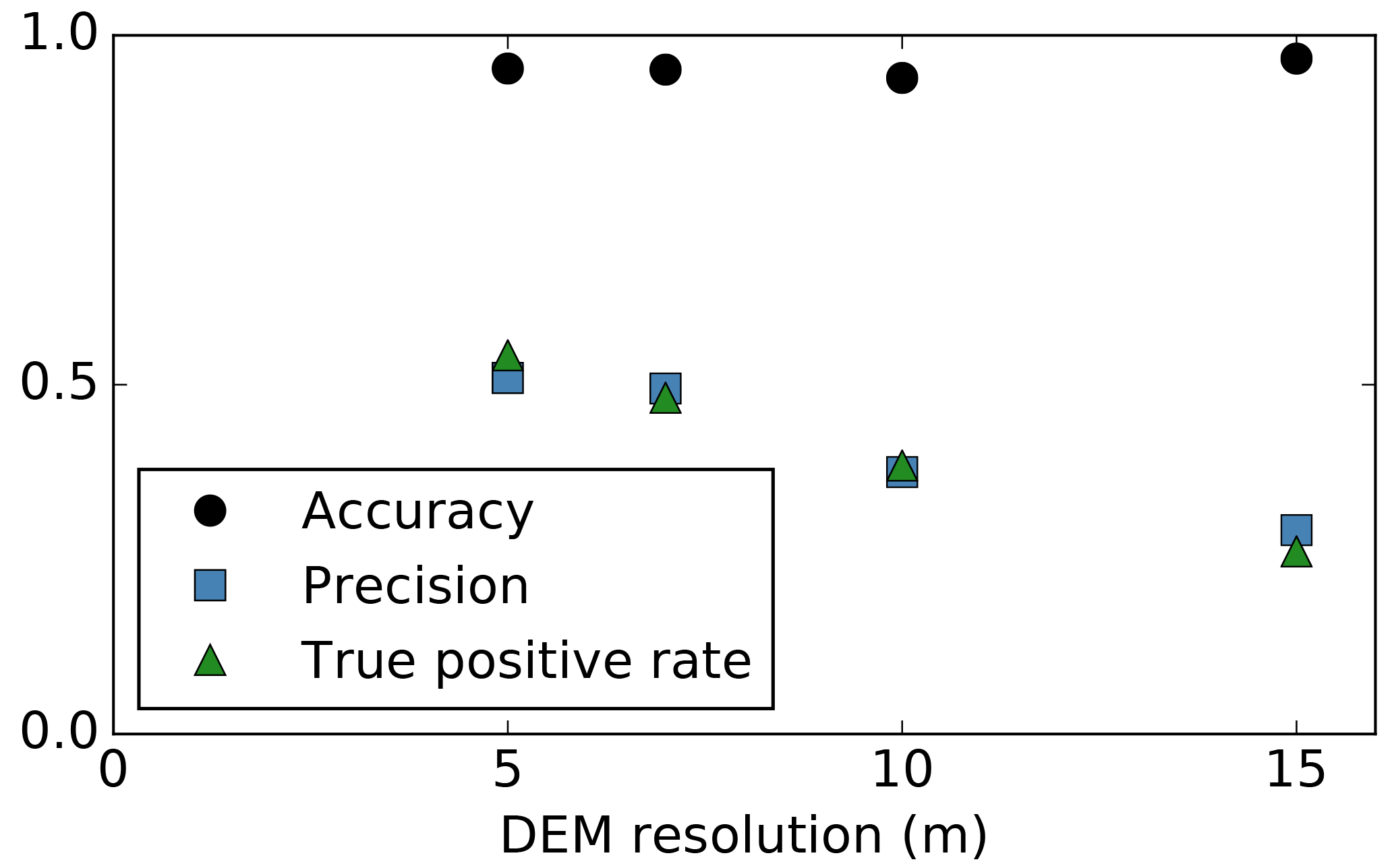
Figure 9 Identical to Fig. 6a, except with TP and FP area removed from the Canwell Glacier spatial domain to test the method on an area that definitively has no ice cliffs. For comparison, dots shown in grey are the black dots in Fig. 6a where TP and FP area are not removed. The curly bracket shows the extension of the curve that is indicative of the presence of steep surface slope areas characteristic of ice cliffs. While the method still identified area (erroneously) as ice cliff, the abrupt termination of the curve with TP and FP area removed was an indication that there were in fact no ice cliffs present.

5.3 What are ice cliffs and how should glaciologists map them?

Throughout this paper the ambiguity of what exactly an ice cliff is has been mentioned. Figure 10 shows an example of an area possibly in the process of becoming an ice cliff. The relief of this medial moraine has facilitated a setting where (geomorphic) mass wasting exceeds englacial debris exhumation and accumulation. The area remains evenly and largely debris-covered, but does appear distinct both in visible and thermal imagery. However, if this is considered sufficient criteria to be defined as an ice cliff, there is no clear edge where ice cliff ends and debris cover begins. We had a difficult time deciding if this feature should be included in the “true” ice cliff dataset, ultimately deciding to include it (and similarly ambiguous features), but also with the caveat in Sect. 3.4 stating that “ice cliffs were liberally outlined”. The slope of the feature identified in Fig. 10 was sufficient to be identified by the automated method as an ice cliff while the surrounding slopes of the medial moraine were not.

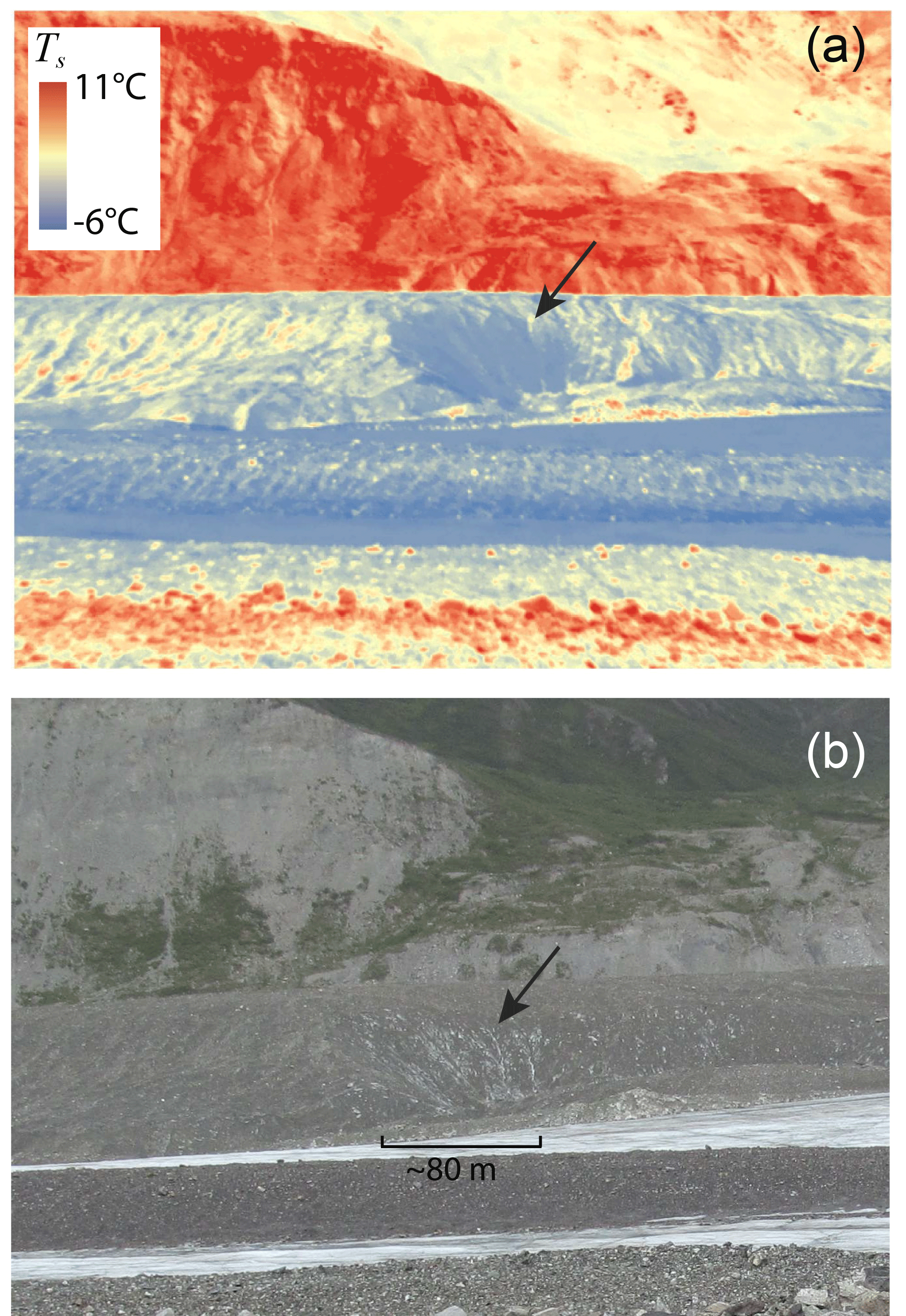
Figure 10 The side of a medial moraine on Canwell Glacier, possibly at an intermediate stage between being classified as an ice cliff or debris-covered area (black arrow in panels a and b). (a) Oblique image of surface temperature (T_s). The sharp boundary between blue and red in the middle of the image separates the top of the medial moraine and the off-glacier valley wall. (b) Oblique visible image of the same feature. Location shown in Fig. 2. Bare ice T_s values below 0 ^∘C are likely due to camera calibration error and/or assuming a constant emissivity for the entire image.

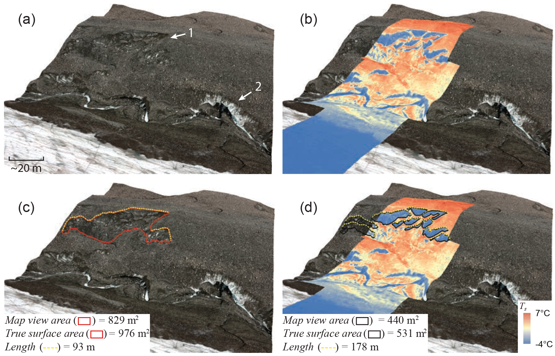
Figure 11 “1” and “2” in panel (a) show a less obvious and a very obvious ice cliff, respectively. When high-resolution surface temperature (T_s) data is draped over ice cliff “1” in panel (b), it becomes very apparent. Panels (c) and (d) demonstrate two common methods for mapping ice cliffs: by area and by tracing the top edge. Bare ice T_s values below 0 ^∘C are likely due to camera calibration error and/or assuming a constant emissivity for the entire image.

Figure 11 shows a second example where an ice cliff could be mapped in detail excluding bands of debris within the ice cliff face (Fig. 11d) or could be mapped more broadly including the debris bands (Fig. 11c). This is a setting where time could be considered when defining an ice cliff as described in Sect. 1. If these debris bands are long term fixtures and there are sufficient data to resolve the individual ice cliff faces, then possibly the detailed mapping is correct. However, if the clasts within the debris bands are transported to the ice cliff margins and not resupplied, the more broad/coarse mapping approach would be appropriate. For this study, we delineated ice cliff(s) “1” from Fig. 11 using the more coarse mapping approach.

While higher resolution data capturing a suite of properties (e.g., visible and surface temperature data) can further resolve what is truly present, it will likely not resolve classification ambiguities (e.g., Figs. 10 and 11), and at the present time these data are not available at large scales. Focus should therefore be more targeted towards mapping consistency. This is best met when automated methods can be applied with sufficient levels of confidence, eliminating technician bias and error.

For both automated and manual mapping methods used in this study, we mapped ice cliffs as a 2-D area (or converted to a 3-D surface). An alternative method to map ice cliffs is to define a line along the ice cliff top edge (Thompson et al., 2016; Watson et al., 2017). Figure 11 provides a comparison of all three methods (3-D surface area, 2-D map-view surface area and 1-D top edge line) and shows that when mapping ice cliffs as a 2- or 3-D area, refined detail leads to a refined (smaller/more accurate) area, while refined detail leads to an expansion of ice cliff top edge length when mapping ice cliffs in 1-D. This suggests that 2- or 3-D area is a more reliable measure and likely more communicative if drawing a comparison with other regions or studies.

6 Conclusions

This study presents a new automated method for mapping ice cliffs within supraglacial debris cover. The method uses glacier outlines and satellite imagery to isolate debris-covered area where ice cliffs might exist and then uses DEM data alone to map ice cliff area. The DEMs used in this study had a spatial resolution of 5 m; however, for future applications of this method with different input DEM sources, we have derived a relation between coarsening DEM resolution and method performance which can help guide anticipated outcomes. The method is designed to accommodate regional variability in ice cliff characteristics by selecting unique surface slope threshold values automatically. The method also attempts to improve performance by explicitly considering the often narrowing ends of ice cliffs. The method was calibrated using data from Canwell Glacier in Alaska, USA, and validated using data from Ngozumpa Glacier in Nepal. The best parameter set for Canwell Glacier produced an ice cliff map with essentially equivalent success to a carefully selected simple surface slope threshold, which itself carried a degree of error with true positive rate and precision both around 0.5. While the application of a simple surface slope threshold is a much easier mapping technique, the selection of a sufficient threshold requires supplemental, high-resolution data due to the rapid increase in error with less ideal threshold selections. The method presented here attempts to automatically mitigate this instability and offer a confident ice cliff map when supplemental data are not available. With no parameter alteration, the method was applied on the other side of the world. Results from Ngozumpa Glacier show a decrease in performance relative to Canwell Glacier where true positive rate is similar, but precision is 19 % less. This is still, however, an ice cliff map with more success than if the carefully selected simple surface slope threshold for Canwell Glacier was assumed to be transferable to Ngozumpa Glacier. Under this assumption, precision is 41 % less and the ice cliff area mapped incorrectly is a factor of 6.93 more than the results for Canwell Glacier. We therefore conclude that simple surface slope thresholds (1) carry a non-trivial degree of error even if carefully selected; and (2) cannot be considered transferable to other regions. In this study we have quantified (1) and presented a method to mitigate (2).

While we only consider two locations, these results offer an idea of how well the method might perform in other regions without supplemental validation data and opens the possibility for deriving ice cliff area at large scales. With a DEM of adequate spatial resolution, which we show is best around 5 m, and sufficient computational capacity, this method could be applied to all glacierized area on Earth. Additionally, applying the method to temporal data will produce a time-lapse evolution of ice cliff formation, cessation, melt patterns and motion through the glacier flow regime. Further validation of this method using ice cliff maps from high-resolution visible, thermal or other data in other regions will help to either support or discredit our claim of wide applicability. Ambiguities defining what exactly an ice cliff is are likely to persist in any technique used to map ice cliffs, but map variance from these ambiguities will become less of a factor if a consistent methodology is used.