Changing pattern of ice flow and mass balance for glaciers discharging into the Larsen A and B embayments, Antarctic Peninsula, 2011 to 2016

We analysed volume change and mass balance of outlet glaciers on the northern Antarctic Peninsula over the periods 2011 to 2013 and 2013 to 2016, using high-resolution topographic data from the bistatic interferometric radar satellite mission TanDEM-X. Complementary to the geodetic method that applies DEM differencing, we computed the net mass balance of the main outlet glaciers using the mass budget method, accounting for the difference between the surface mass balance (SMB) and the discharge of ice into an ocean or ice shelf. The SMB values are based on output of the regional climate model RACMO version 2.3p2. To study glacier flow and retrieve ice discharge we generated time series of ice velocity from data from different satellite radar sensors, with radar images of the satellites TerraSAR-X and TanDEM-X as the main source. The study area comprises tributaries to the Larsen A, Larsen Inlet and Prince Gustav Channel embayments (region A), the glaciers calving into the Larsen B embayment (region B) and the glaciers draining into the remnant part of the Larsen B ice shelf in Scar Inlet (region C). The glaciers of region A, where the buttressing ice shelf disintegrated in 1995, and of region B (ice shelf break-up in 2002) show continuing losses in ice mass, with significant reduction of losses after 2013. The mass balance numbers for the grounded glacier area of region A are −3.98 ± 0.33 Gt a⁻¹ from 2011 to 2013 and −2.38 ± 0.18 Gt a⁻¹ from 2013 to 2016. The corresponding numbers for region B are −5.75 ± 0.45 and −2.32 ± 0.25 Gt a⁻¹. The mass balance in region C during the two periods was slightly negative, at −0.54 ± 0.38 Gt a⁻¹ and −0.58 ± 0.25 Gt a⁻¹. The main share in the overall mass losses of the region was contributed by two glaciers: Drygalski Glacier contributing 61 % to the mass deficit of region A, and Hektoria and Green glaciers accounting for 67 % to the mass deficit of region B. Hektoria and Green glaciers accelerated significantly in 2010–2011, triggering elevation losses up to 19.5 m a⁻¹ on the lower terminus during the period 2011 to 2013 and resulting in a mass balance of −3.88 Gt a⁻¹. Slowdown of calving velocities and reduced calving fluxes in 2013 to 2016 coincided with years in which ice mélange and sea ice cover persisted in proglacial fjords and bays during summer.

1 Introduction

The disintegration of the ice shelves in Prince Gustav Channel and the Larsen A embayment in January 1995 (Rott et al., 1996) and the break-up of the northern and central sections of the Larsen B embayment in March 2002 (Rack and Rott, 2004; Glasser and Scambos, 2008) triggered near-immediate acceleration of the outlet glaciers previously feeding the ice shelves, resulting in major mass losses due to increased ice discharge (Rott et al., 2002; De Angelis and Skvarca, 2003; Scambos et al., 2004, 2011). Precise, spatially detailed data on flow dynamics and mass balance of these glaciers after ice-shelf disintegration are essential for understanding the complex glacier response to the loss of ice shelf buttressing, as well as for learning about the processes controlling the adaptation to new boundary conditions. Furthermore, due to the complex topography of this region, spatially detailed data on glacier surface elevation change and mass balance are key for reducing the uncertainty of northern Antarctic Peninsula (API) contributions to sea level rise.

Several studies dealt with mass balance, acceleration and thinning of glaciers after the disintegration of the Larsen A and B ice shelves, with the majority focusing on glaciers of the Larsen B embayment. A complete, detailed analysis of changes in ice mass was performed by Scambos et al. (2014) for 33 glacier basins covering the API mainland and adjoining islands north of 66^∘ S, using a combination of digital elevation model (DEM) differencing from optical stereo satellite images and repeat-track laser altimetry from the Ice, Cloud, and land Elevation Satellite (ICESat). The DEM difference pairs cover the periods 2001–2006, 2003–2008 and 2004–2010 for different sections of the study area and are integrated with ICESat data from the years 2003 to 2008. A detailed analysis of surface elevation change and mass depletion for API outlet glaciers draining into the Larsen A, Larsen Inlet and Prince Gustav Channel (PGC) embayments from 2011 to 2013 was reported by Rott et al. (2014), based on topographic data from the TanDEM-X/TerraSAR-X satellite formation. With a mass balance of −4.21 ± 0.37 Gt a⁻¹ during 2011–2013 these glaciers were still largely out of balance, although the loss rate during this period was diminished by 27 % compared to the loss rate reported by Scambos et al. (2014) for 2001 to 2008. Studies on frontal retreat, ice velocities and ice discharge, based on remote sensing data from the period 1992 to 2014, are reported by Seehaus et al. (2015) for the Dinsmoor–Bombardier–Edgeworth glacier system previously feeding the Larsen A ice shelf and by Seehaus et al. (2016) for the glaciers of Sjögren Inlet previously feeding the PGC ice shelf.

As observed previously for Larsen A (Rott et al., 2002), the major outlet glaciers to the Larsen B embayment started to accelerate and thin immediately after the collapse of the ice shelf (Rignot et al., 2004; Scambos et al., 2004; De Rydt et al., 2015). The patterns of acceleration, thinning and change in the frontal position have been variable in time and space. After strong acceleration during the first years, some of the main glaciers slowed down significantly after 2007, resulting in a major decrease in calving fluxes. Other glaciers continued to show widespread fluctuations in velocity, with periods of major frontal retreat alternating with stationary positions or intermittent frontal advance (Wuite et al., 2015). The remnant section of the Larsen B ice shelf in Scar Inlet started to accelerate soon after the central and northern sections of the ice shelf broke away, triggering modest acceleration of the main glaciers flowing into the Scar Inlet ice shelf (Wuite et al., 2015; Khazendar et al., 2015).

Several publications reported ice export and mass balance of the Larsen B glaciers. Shuman et al. (2011) derived surface elevation change from optical stereo satellite imagery and laser altimetry of ICESat and the Airborne Topographic Mapper (ATM) of NASA's IceBridge programme. For the period 2001 to 2006 they report a combined mass balance of −8.4 ± 1.7 Gt a⁻¹ for the glaciers discharging into the Larsen B embayment and Scar Inlet, excluding ice lost by frontal retreat. ICESat and ATM altimetry measurements spanning 2002–2009 show for the lower Crane Glacier a period of very rapid drawdown between September 2004 and September 2005, bounded by periods of more moderate rates of surface lowering (Scambos et al., 2011). Rott et al. (2011) derived velocities and ice discharge of the nine main Larsen B glaciers in a pre-collapse state (1995 and 1999) and for 2008–2009, estimating the mass balance of these glaciers in 2008 at −4.34 ± 1.64 Gt a⁻¹. Berthier et al. (2012) report a mass balance of −9.04 ± 2.01 Gt a⁻¹ for Larsen B glaciers, excluding Scar Inlet, for the period 2006 to 2010–2011, based on altimetry and optical stereo imagery. Scambos et al. (2014) analysed changes in ice mass from ICESat data spanning September 2003 to March 2008 and stereo image DEMs spanning 2001–2002 to 2006. They report a combined mass balance of −7.9 Gt a⁻¹ for the tributaries of the Larsen B embayment and −1.4 Gt a⁻¹ for the tributaries to the Scar Inlet ice shelf. Wuite et al. (2015) report strongly reduced calving fluxes for the main outlet glaciers during the period 2010 to 2013 compared to the first few years after ice shelf collapse.

We use high-resolution data on surface topography derived from synthetic aperture radar interferometry (InSAR) satellite measurements for retrieving changes in glacier volume and estimating glacier mass balance over well-defined epochs for API outlet glaciers along the Weddell Sea coast between PGC and Jason Peninsula. In addition, we generate ice velocity maps to study the temporal evolution of ice motion and derive the ice discharge for the major glacier drainage basins. We also compute the mass balance by means of the mass budget method, quantifying the difference between glacier surface mass balance (SMB) and the discharge of ice into the ocean or across the grounding line to an ice shelf. The SMB estimates are obtained from the output of the regional atmospheric climate model RACMO version 2.3p2 at a grid size of ∼ 5.5 km (van Wessem et al., 2016, 2017).

Volume change and mass balance of glaciers discharging into the PGC, Larsen Inlet and Larsen A embayments were derived by Rott et al. (2014) for the period 2011 to 2013, applying TanDEM-X DEM differencing. Here we extend the observation period for the same glacier basins by covering the time span 2013 to 2016. Furthermore, we present time series of surface velocity starting in 1993–1995 in order to relate the recent flow behaviour to pre-collapse conditions.

For glaciers of the Larsen B embayment we generated maps of surface elevation change by TanDEM-X DEM differencing for the periods 2011 to 2013 and 2013 to 2016. From these maps we derived mass changes at the scale of individual glacier drainage basins. In addition, we obtained mass balance estimates for the eight main glaciers using the mass budget method and compare the results of the two independent methods. A detailed analysis of surface velocities of the Larsen B glaciers for the period 1995 to 2013 was presented by Wuite et al. (2015). We extend the time series to cover glacier velocities up to 2016.

These data sets disclose large temporal and spatial variability in ice flow and surface elevation change between different glacier basins and show ongoing loss of grounded ice. This provides a valuable basis for studying factors responsible for instability and downwasting of glaciers and for exploring possible mechanisms of adaptation to new boundary conditions.

2 Data and methods

2.1 DEM differencing using TanDEM-X interferometric SAR data

The study is based on remote sensing data from various satellite missions. We applied DEM differencing using interferometric SAR data (InSAR) of the TanDEM-X mission to map the surface elevation change and retrieve the mass balance for 24 catchments on the API east coast between PGC and Jason Peninsula (Table S1 in the Supplement). Large glaciers are retained as single catchments, whereas smaller glaciers and glaciers that used to share the same outlet are grouped together. To separate glacier drainage basins inland of the frontal areas, the glacier outlines of the Glaciology Group, University of Swansea are used, which are available from the GLIMS database (Cook et al., 2014). We updated the glacier fronts for several dates of the study period using TerraSAR-X, TanDEM-X and Landsat 8 images. Catchment outlines and frontal positions in 2011, 2013 and 2016 are plotted in a Landsat image of 29 October 2016 (Figs. S1 and S2 in the Supplement).

The TanDEM-X mission (TDM) employs a bistatic interferometric configuration of the two satellites TerraSAR-X and TanDEM-X flying in close formation (Krieger et al., 2013). The two satellites together form a single-pass synthetic aperture radar (SAR) interferometer, enabling the acquisition of highly accurate cross-track interferograms that are not affected by temporal decorrelation and variations in atmospheric phase delay. The main objective of the mission is the acquisition of a global DEM with high accuracy. The 90 % relative point-to-point height accuracy for moderate terrain is ±2 m at 12 m posting (Rossi et al., 2012; Rizzoli et al., 2012). Higher relative vertical accuracy can be achieved for measuring elevation change over time.

Our analysis of elevation change is based on DEMs derived from interferograms acquired by the TanDEM-X mission in mid-2011, -2013 and -2016. SAR data takes from descending satellite orbits, acquired in 2013 and 2016, cover the API east coast glaciers between 64^∘ S and the Jason Peninsula, as well as parts of the west coast glaciers (Fig. S3). For 2011 we processed data takes covering the Larsen B glaciers. Over the Larsen A glaciers TDM data from 2011 and 2013 had been processed in an earlier study to derive surface elevation change (SEC). The mid-beam incidence angle of the various tracks varies between 36.1 and 45.6^∘. The height of ambiguity (HoA, the elevation difference corresponding to a phase cycle of 2π) varies between 20.6 and 68.9 m, providing good sensitivity to elevation (Rott, 2009) (Table S2). Only track A has a larger HoA and thus less height sensitivity; this track extends along the west coast and covers only a very small section of study glaciers along the Weddell coast.

We used the operational Integrated TanDEM-X Processor (ITP) from the German Aerospace Center (DLR) to process the raw bistatic SAR data from the individual tracks into so-called raw DEMs (Rossi et al., 2012; Abdel Jaber, 2016). In the production line for the global DEM, which also uses the ITP, raw DEMs are intermediate products generated before DEM mosaicking. An option recently added to the ITP foresees the use of reference DEMs to support raw DEM processing (Lachaise and Fritz, 2016). We applied this option to generate the raw DEMs by subtracting the phase of the simulated reference DEM from the interferometric phase of the corresponding scene. The recently released TanDEM-X global DEM with a posting of 0.4 arcsec was used as the main reference DEM. Although the relative elevation in output is not related to the reference DEM, the presence of inconsistencies in the reference DEM may lead to artefacts in the output DEM. Therefore some preparatory editing was performed: unreliable values were removed based on the provided consistency mask of the global DEM and visual analysis and were substituted by data from the Antarctic Peninsula DEM of Cook et al. (2012). The phase difference image, which has a much lower fringe frequency, is unwrapped and summed up with the simulated phase image. This option provides a robust phase-unwrapping performance for compiling the individual DEMs. By subtracting the two DEMs and accounting for the appropriate time span we obtain a surface elevation rate of change map, with horizontal posting at about 12 m × 12 m.

For estimating the uncertainty of the TanDEM SEC maps we use a fully independent data set acquired during NASA IceBridge campaigns that became available after the production of the TDM SEC maps had been completed (Sect. S3 in the Supplement). Surface elevation rate of change data (dh∕dt, product code IDHDT4) derived from Airborne Topographic Mapper (ATM) swathes, acquired on 14 November 2011 and 10 November 2016, cover longitudinal profiles on six of our study glaciers (Studinger, 2014, updated 2017). Each IDHDT4 data record corresponds to an area where two ATM lidar swathes have co-located measurements. The IDHDT4 data are provided as discrete points representing a 250 m × 250 m surface area and are posted with about 80 m along-track spacing. We compare mean values of cells comprising 7 × 7 TDM dh∕dt pixels (12 m × 12 m pixel size) with the corresponding IDHDT4 points. Even though the start and end dates of the TDM and ATM data sets differ by a few months, the agreement in dh∕dt is very good. The root mean square differences (RMSDs) of the data points range from 0.14 to 0.35 m a⁻¹ for the different glaciers, and the mean difference of the ATM and TDM data sets is $\text{d}h/\text{d}t=-\mathrm{0.08}$ m a⁻¹ (Table S3). For the error analysis we assume that the differences result from uncertainties in both data sets. The resulting RMSE for the TDM dh∕dt cells is 0.20 m a⁻¹ over the 5-year time span, and 0.39 and 0.58 m a⁻¹ for the 3- and 2-year time spans, respectively.

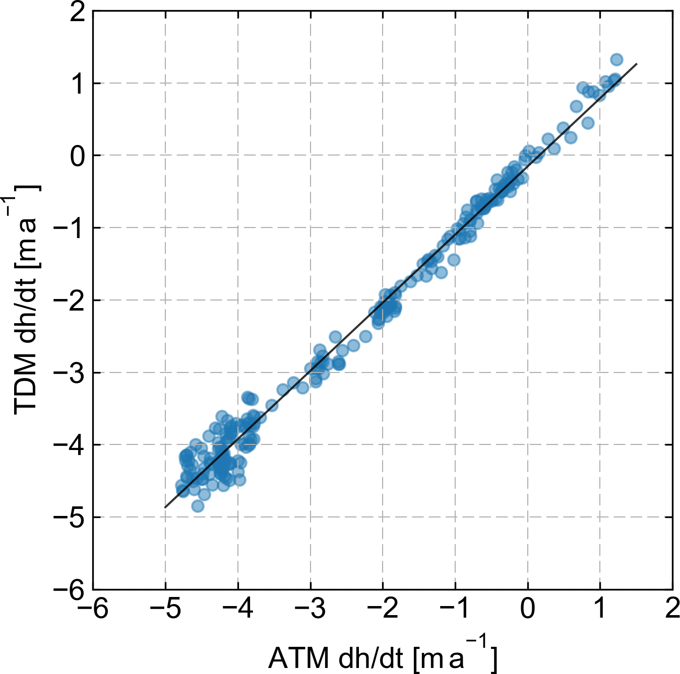
Figure 1 Scatter plot of measurements of surface elevation change (dh∕dt) 2016–2011 on the central flow line of Crane Glacier based on IceBrigde ATM and TanDEM-X elevation data. The line shows the linear fit.

In order to demonstrate the concordance of the dh∕dt data sets, in Fig. 1 we show a scatter plot of ATM and TDM dh∕dt values from the central flow line on Crane Glacier. The TDM dh∕dt data are derived from DEMs from 30 June 2011 and 7 August 2016. Because of the time shifts between ATM and TDM data acquisitions we start with the comparison 5 km inland of the front in order to avoid the impact of the shifting glacier front, of floating section of the terminus and of moving crevasse zones. The data in the figure include the points along the flow line as far as the upper end of the ATM profile at 1000 m elevation. In spite of the time shift the agreement between the two data sets is excellent; the coefficient of determination (R²) is 0.98.

The agreement between the lidar and radar dh∕dt data indicates that radar penetration is not an issue for deriving elevation change from the SAR based DEMs of this study. This can be attributed to the close agreement of the viewing angles in the corresponding SAR repeat data, acquired from the same orbit track and beam and to the consistency of radar propagation properties in the snow and firn bodies. The latter point follows from the similarity of the backscatter coefficients of the corresponding scenes, with differences between the two dates staying below 1 dB. The radar backscatter coefficient can be used as an indicator of stability of the structure and radar propagation properties of a snow/ice medium which determine the signal penetration and the offset of the scattering phase centre versus the surface (Rizzoli et al., 2017). The TDM SAR backscatter images have high radiometric accuracy (absolute radiometric accuracy 0.7 dB, relative radiometric accuracy 0.3 dB), very suitable for quantifying temporal changes in backscatter (Schwerdt et al., 2010; Walter Antony et al., 2016).

The main outlet glaciers of the study area arise from the plateaus along the central API ice divide. The plateaus stretch across elevations between about 1500 and 2000 m a.s.l. A steep escarpment, dropping about 500 m in elevation, separates the plateau from the individual glacier streams and cirques. The high-resolution SEC maps, shown in Figs. 2, 6 and 7, cover the areas below the escarpment excluding parts of the steep rock- and ice-covered slopes along the glacier streams. These gaps are due to the particular SAR observation geometry, with slopes facing towards the illuminating radar beam appearing compressed (foreshortening) or being affected by the superposition of dual or multiple radar signals (layover) (Rott, 2009). On areas with gentle topography and on slopes facing away from the radar beam (back-slopes) the surface elevation and its change can be derived from the interferometric SAR images. In order to fill the gaps in areas of foreshortening and layover, we checked the topographic change on the back-slopes. The TDM data set includes SEC data for 38 individual sections on the back-slopes with mean slope angles ≥ 20^∘, covering a total area of 787 km². The mean dh∕dt value of these slopes is −0.054 m a⁻¹. The satellite-derived velocity maps show surface velocities < 0.02 m d⁻¹ on any slope area, indicating that dynamic effects are insignificant for mass turnover. This explains the observed stability of surface topography.

There are also some gaps in the SEC maps on the plateau above the escarpment. The TDM SEC analysis covers substantial parts (all together 2013 km²) of the ice plateaus between 1500 and 2000 m; the mean dh∕dt is −0.012 m a⁻¹. No distinct spatial pattern is evident. Considering the small change in surface elevation in the available data samples of the ice plateau and on the slopes, we assume stationary conditions for the unsurveyed slopes and the central ice plateau. To estimate uncertainty for these areas we assume a bulk uncertainty $\text{d}h/\text{d}t=\pm$0.10 m a⁻¹ for the error budget of elevation change derived from DEMs spanning 3 years and $\text{d}h/\text{d}t=\pm$0.15 m a⁻¹ for DEMs spanning 2 years (Sect. S3).

2.2 Ice velocity maps and calving fluxes

We generated maps of glacier surface velocity for several dates of the study period from radar satellite images, extending the available velocity time series up to 2016. The main data for the recent velocity maps are repeat-pass SAR images of the satellites TerraSAR-X and TanDEM-X. Gaps in these maps, primarily in the slow-moving interior, are filled with velocities derived from SAR images of Sentinel-1 (S1) and of the Phased Array L-band SAR (PALSAR) on ALOS. We applied offset tracking to derive two-dimensional surface displacements in radar geometry and projected these onto the glaciers surfaces defined by the Advanced Spaceborne Thermal Emission and Reflection Radiometer (ASTER)-based Antarctic Peninsula digital elevation model (API-DEM) of Cook et al. (2012). The velocity data set comprises the three components of the surface velocity vector in Antarctic polar stereographic projection resampled to a 50 m grid.

The TerraSAR-X/TanDEM-X velocity maps are based on SAR strip map mode images of 11-day repeat-pass orbits, using data spanning one or two repeat cycles. Due to the high spatial resolution of the images (3.3 m along the flight track and 1.2 m in radar line-of-sight) velocity gradients are well resolved. Wuite et al. (2015) estimated the uncertainty of velocity maps (magnitude) of the Larsen B glaciers derived from TerraSAR-X 11-day repeat-pass images at ±0.05 m d⁻¹.

Regarding S1 we use single-look complex (SLC) Level 1 products acquired in interferometric wide (IW) swath mode, with nominal spatial resolution of 20 m × 5 m (Torres et al., 2012; Nagler et al., 2015). Images of the Sentinel-1A satellite in a 12-day repeat cycle cover the study region from December 2014. Since September 2016 the area has also been covered by the Sentinel-1B satellite, providing a combined S1 data set with 6-day repeat coverage. In order to check the impact of combining different ice velocity products, we compared TerraSAR-X/TanDEM-X velocity maps of the study area, resampled to 200 m, with S1 velocity maps using data sets with a maximum time difference of 10 days. The overall mean bias (S1 – TerraSAR-X/TanDEM-X) between the two data sets (sample 570 000 points) is 0.011 m d⁻¹ for the velocity component V_e (easting) and −0.002 m d⁻¹ for V_n (northing), the RMSD is 0.175 m d⁻¹ for V_e and 0.207 m d⁻¹ for V_n. The RMSD values for the TerraSAR-X and Sentinel-1 velocity product are mainly due to the different spatial resolutions of the sensors. The good agreement of the mean velocity values indicates that velocity data from the two missions can be easily merged.

In addition to the recently generated velocity products we use velocity data from earlier years to support the scientific interpretations which were derived from SAR data from various satellite missions, including ERS-1, ERS-2, Envisat ASAR and ALOS PALSAR (Rott et al., 2002, 2011, 2014; Wuite et al., 2015).

In order to obtain mass balance estimates using the mass budget method, we compute the mass flux F across a gate of width Y [m] at the calving front or grounding line according to

$$F_Y={\mathit{\rho }}_{\text{i}}\underset{\mathrm{0}}{\overset{Y}{\int }}\left[u_{\text{m}}\left(y\right)H\left(y\right)\right]\text{d}y.$$

ρ_i is the density of ice, u_m is the mean velocity of the vertical ice column perpendicular to the gate, and H is the ice thickness. We use an ice density of 900 kg m⁻³ to convert the ice volume into mass. From the similarity of the radar backscatter coefficients in the 2011 and 2016 TanDEM-X images we can exclude significant changes in the structure and density of the snow/firn column. The good agreement between the IceBridge lidar and the TanDEM-X dh∕dt values also indicates stability of the structure and density of the snow/ice medium. Therefore the possible error due to density changes in the vertical column is negligible compared to the uncertainty in dh∕dt (details in Sect. S3.2). For calving glaciers full sliding is assumed across calving fronts, so that u_m corresponds to the surface velocity, u_s, obtained from satellite data. For glaciers discharging into the Scar Inlet ice shelf we estimated the ice deformation at the flux gates applying the laminar flow approximation (Paterson, 1994). The resulting vertically averaged velocity for these glaciers is u_m=0.95u_s. The ice thickness at the flux gates is obtained from various sources. For some glaciers sounding data on ice thickness are available, measured either by in situ or airborne radar sounders (Farinotti et al., 2013, 2014; Leuschen et al., 2010, updated 2016). For glaciers with floating terminus the ice thickness is deduced from the height above sea level, applying the flotation criterion.

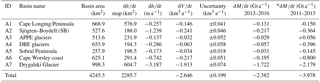
Table 1 Rates of surface elevation change, volume change and mass balance by means of TDM DEM differencing 2013 to 2016, for glacier basins discharging into Prince Gustav Channel, Larsen Inlet and Larsen A embayment. dh∕dt is the mean rate of elevation change in the area covered by the high-resolution map (Fig. 2). The basin area refers to ice front positions delineated in TanDEM-X images of 16 July, 27 July, 18 August 2016. The rates of ice volume change (dV∕dt) and total mass balance (dM∕dt) refer to grounded ice. ^* dM∕dt 2011–2013 for grounded areas of basins A1 to A7 from the TDM SEC analysis by Rott et al. (2014).

The uncertainty estimate for mass balance at basin scale, derived by means of the mass budget method, accounts for uncertainties of SMB and for uncertainties in flow velocity and ice thickness at the flux gates (Sect. S3.2). For uncertainty estimates of mass fluxes we assume ±10 % error in the cross section area of glaciers with GPR data across or close to the gates and ±15 % for glaciers where the ice thickness is deduced from frontal height above flotation. The velocities used for computing calving fluxes are exclusively derived from TerraSAR-X and TanDEM-X repeat-pass data. For velocities across the gates we assume ±5 % uncertainty. For surface mass balance at basin scale, based on RACMO output, the uncertainty is estimated at ±15 %.

3 Elevation change and mass balance of glaciers north of Seal Nunataks

3.1 Elevation change and mass balance by DEM differencing

The map of surface elevation change dh∕dt from June–July 2013 to July–August 2016 for the glacier basins discharging into PGC, Larsen Inlet and Larsen A embayment is shown in Fig. 2. The numbers on elevation change, volume change and mass balance, excluding floating glacier areas, are specified in Table 1. As explained in Sect. 2.1, for areas not displayed on this map (steep radar fore-slopes and the ice plateau above the escarpment) the available data indicate minimal changes in surface elevation so that stable surface topography is assumed for estimating the net mass balance.

Figure 2 Map of surface elevation change dh∕dt (SEC) (m a⁻¹) June–July 2013 to July–August 2016 on glaciers north of Seal Nunataks (SN). AI – Arrol Icefall, CL – Cape Longing, CW – Cape Worsley. L-A – Larsen A embayment, LI – Larsen Inlet, PGC – Prince Gustav Channel.

Table 2 (a) Area extent of floating ice in 2016; (b) and (c)  show rate of surface elevation change and volume change 2013 to 2016 of floating ice; (a–c) exclude the areas of frontal advance; (d) and (e) show the extent and volume of frontal advance (+) or retreat (−) areas.

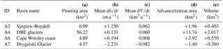
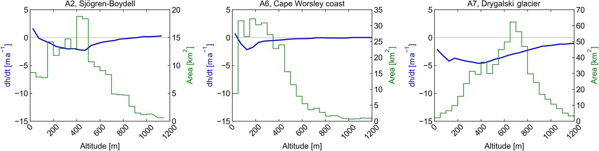
Figure 3 Rate of glacier surface elevation change dh∕dt (in m a⁻¹) from 2013 to 2016 versus altitude in 50 m intervals for basins A2, A6 and A7. Green line: hypsometry of surveyed glacier area in km².

For glaciers with major sections of floating ice and frontal advance or retreat, the extent, SEC and volume change (including the subaqueous part) of the floating area and the advance/retreat area and volume are specified in Table 2. The area extent of floating ice is inferred from the reduced rate of SEC compared to grounded ice, using the height above sea level as an additional constraint. Dinsmoor–Bombardier–Edgeworth glaciers (DBE, basin A4) had the largest floating area (56.2 km²), extending about 8 km into a narrow fjord and also showed the largest frontal advance (11.7 km²) between 2013 and 2016.

The mass depletion of grounded ice in the basins A1 to A7 ($B_{\text{n}}=-\mathrm{2.38}$ Gt a⁻¹) during the period 2013 to 2016 amounts to 60 % of the 2011 to 2013 value ($B_{\text{n}}=-\mathrm{3.98}$ Gt a⁻¹ for the grounded areas; Rott et al., 2014). The mass deficit is dominated by Drygalski Glacier ($B_{\text{n}}=-\mathrm{1.72}$ Gt a⁻¹ for 2013 to 2016 and −2.18 Gt a⁻¹ for 2011 to 2013). A decline of mass losses between the first and second period is observed for all basins except A3 (Albone, Pyke, Polaris, Eliason glaciers, APPE) in Larsen Inlet, which was approximately in a balanced state from 2011 to 2016 (Table 1, Fig. 2).

The altitude dependence of elevation change (dh∕dt) for the three basins with the largest mass deficit is shown in Fig. 3. Positive values in the lowest elevation zone of Basin A2 and A6 are due to frontal advance. The areas close to the fronts include partly floating ice so that the observed SEC is smaller than on grounded areas further upstream. The largest loss rates are observed in elevation zones several km inland of the front.

3.2 Flow velocities, calving fluxes and mass balance using the mass budget method

Data on flow velocities provide, on one hand, input for deriving calving fluxes. On the other hand they provide information for studying the dynamic response of the glaciers. Figure 4 shows maps of surface velocities in 2011 and 2016, derived from TerraSAR-X and TanDEM-X 11-day repeat-pass images and a map of the difference in velocity between October–November 1995 and 2016. Insets show the velocity difference from 2011 to 2016 for the main glaciers that were subject to slowdown. The 1995 velocity map was derived from interferometric 1-day repeat-pass data on crossing orbits from the satellites ERS-1 and ERS-2 (map shown in Fig. S3 of Rott et al., 2014, Supplement). In October–November 1995, 10 months after the ice shelf collapse, the velocities at the calving fronts had already accelerated significantly compared to pre-collapse conditions (Rott et al., 2002). Between 2011 and 2016 the flow velocities slowed down significantly. Even so, in 2016 the terminus velocities of the major outlet glaciers still exceeded the November 1995 velocities.

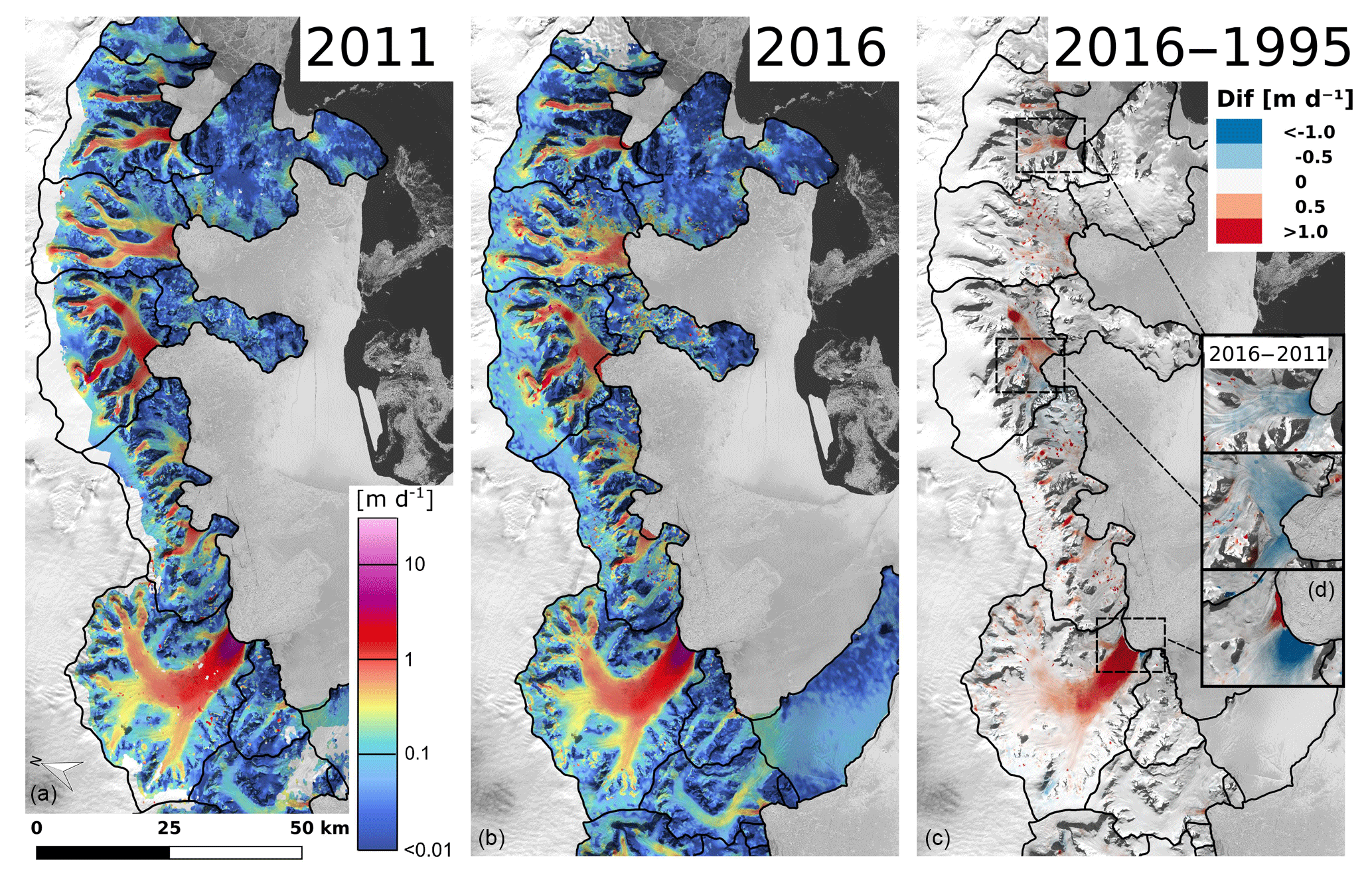
Figure 4 Magnitude of ice velocity (m d⁻¹) 2011 (a) and 2016 (b) derived from TerraSAR-X and TanDEM-X data. Gaps in 2011 filled with PALSAR data and in 2016 filled with Sentinel-1 data. (c) Map of velocity difference between 2016 and 1995 (October–November). Insets: velocity difference between 2016 and 2011 for Sjögren, DBE and Drygalski glaciers.

Table 3 Mean specific surface mass balance, b_n, for 2011 to 2016, and rates of surface mass balance (SMB), calving flux (CF) and mass balance (MB) using the mass budget method in Gt a⁻¹ for the periods 2011 to 2013 and 2013 to 2016 for outlet glaciers north of Seal Nunataks.

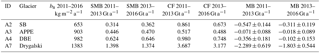
Figure 5 Surface velocities along the central flow lines of Drygalski, Edgeworth and Sjögren glaciers and their frontal positions on different dates (month/year). The x and y scales are different for individual glaciers. Vertical lines show positions of the calving front. The insets show velocities in the centre of the flux gates.

Details on velocities along the central flow lines of Drygalski, Edgeworth and Sjögren glaciers and the position of calving fronts are shown in Fig. 5 for different dates between 1993–1995 and 2016. The distance along the x axis refers to the 1995 grounding line retrieved from ERS-1/ERS-2 InSAR data (Rott et al., 2002). The front of the three glaciers has retreated by several kilometres since 1995, with the largest retreat (11 km) by Sjögren Glacier in 2012. Between 2013 and 2016 the front of Edgeworth Glacier advanced by 1.5 km and the front of Sjögren Glacier by 0.5 km.

The velocity of Sjögren Glacier decreased gradually from 2.9 m d⁻¹ in August 2009 to 1.5 m d⁻¹ in October 2016, referring to the centre of the 2009 front. The calving velocity on Edgeworth Glacier in the centre of the flux gate decreased from 2.5 m d⁻¹ in October 2008 to 1.1 m d⁻¹ in August 2016. The rate of deceleration between 2013 and 2016 was particularly pronounced at the lowest 6 km of the terminus where the ice was ungrounded. For Drygalski Glacier we also show pre-collapse velocities (January 1993), derived from 35-day ERS-1 repeat-pass images by offset tracking. In November 1995 the glacier front was located near the pre-collapse grounding line, but the flow acceleration had already propagated 10 km upstream of the front. Due to rapid flow the phase of the 31 October–1 November 1995 ERS-1/ERS-2 InSAR pair is decorrelated on the lowest 2 km, prohibiting interferometric velocity retrieval. Velocities in January 1999 and November 2015 are similar, with 7.0 m d⁻¹ at the location of the 2015 glacier front. Velocities were lower in 2007 to 2009 and higher in 2011 to 2014, reaching 8.8 m d⁻¹ in November 2011.

The recent period of abating flow velocities coincides with years in which the sea ice cover persisted during summer. Time series of satellite SAR images show open water in front of the glaciers during several summers up to 2008–2009 and again in the summers of 2010–2011 and 2011–2012. Ice mélange and sea ice persisted all year round from winter 2012 onwards. Open leads in summer and the gradual drift of ice that calved off from the glaciers indicate moderate movement of sea ice.

Slowdown of calving velocities is the main cause for reduced mass deficits during the period 2013 to 2016 compared to previous years. Numbers on calving fluxes for 2011 to 2013 and 2013 to 2016 and the mass balance, derived by the mass budget method (MBM), are specified for four main glacier basins in Table 3. To derive the calving flux (CF) for each period a linear interpolation between the fluxes at the start date and end date of the period is applied, including a correction for the time lag between ice motion and topography data. If velocity data are available on additional dates in between, these are also taken into account for temporal interpolation. Whereas the SMB values between the periods 2011 to 2013 and 2013 to 2016 differ only by 2 %, the combined annual calving flux of the four glaciers is reduced by 16 % from 2013 to 2016 (Table 3). The decrease is even more pronounced when calving fluxes of individual dates in 2011, 2013 and 2016 are compared. On Drygalski Glacier the calving flux decreased from 4.03 Gt a⁻¹ in November 2011 to 3.34 Gt a⁻¹ in December 2013 and 2.92 Gt a⁻¹ in September 2016, a decrease by 28 % over the 5 years.

The differences in the mass balance by TDM SEC (Table 1) and MBM (Table 3) are within the specified uncertainty. For MBM the mass balance of the four glaciers sums up to −3.26 Gt a⁻¹ for 2011 to 2013 and −2.23 Gt a⁻¹ for 2013 to 2016. The corresponding numbers from SEC analysis, after adding or subtracting the subaqueous mass changes, are −3.01 and −1.99 Gt a⁻¹ for the two periods.

For Drygalski Glacier the mass balance numbers for the two periods are −2.29 and −1.80 Gt a⁻¹ by MBM, versus −2.18 and −1.80 Gt a⁻¹ (including the subaqueous part) by TDM SEC analysis. The good agreement of the MBM and SEC mass balance values for Drygalski Glacier backs up the RACMO estimate for SMB with specific net balance b_n=1383 kg m⁻² a⁻¹. For the period 1980 to 2016 the mean SMB for Drygalski Glacier by RACMO is 1.35 Gt a⁻¹ (b_n=1342 kg m⁻² a⁻¹). This is more than twice the ice mass flux across the grounding line in a pre-collapse state (0.58 Gt a⁻¹) obtained as model output by Royston and Gudmundsson (2016), which would imply a highly positive mass balance taking RACMO SMB as reference for mass input. Velocity measurements in October–November 1994 at stakes on the Larsen A ice shelf downstream of Drygalski Glacier show values that are close to the average velocity of the 10-year period 1984 to 1994 (Rott et al., 1998; Rack et al., 1999). This supports the assumption that the Larsen A tributary glaciers were approximately in a balanced state before ice shelf collapse.

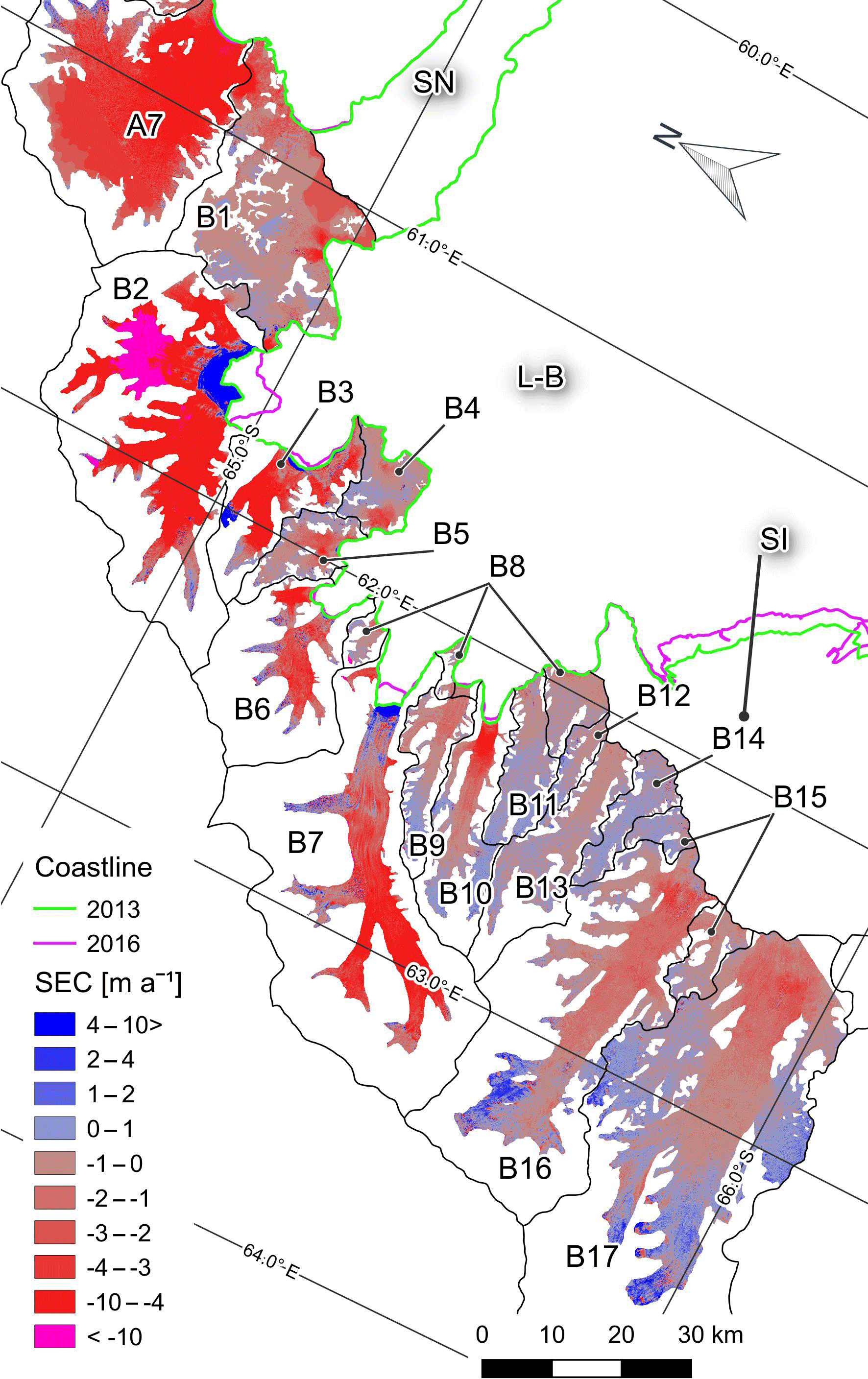
Figure 6 Map of surface elevation change (SEC, m a⁻¹) from May–June 2011 to June–July 2013 on glaciers of the Larsen B embayment (L-B). SN – Seal Nunataks. SI – Scar Inlet ice shelf.

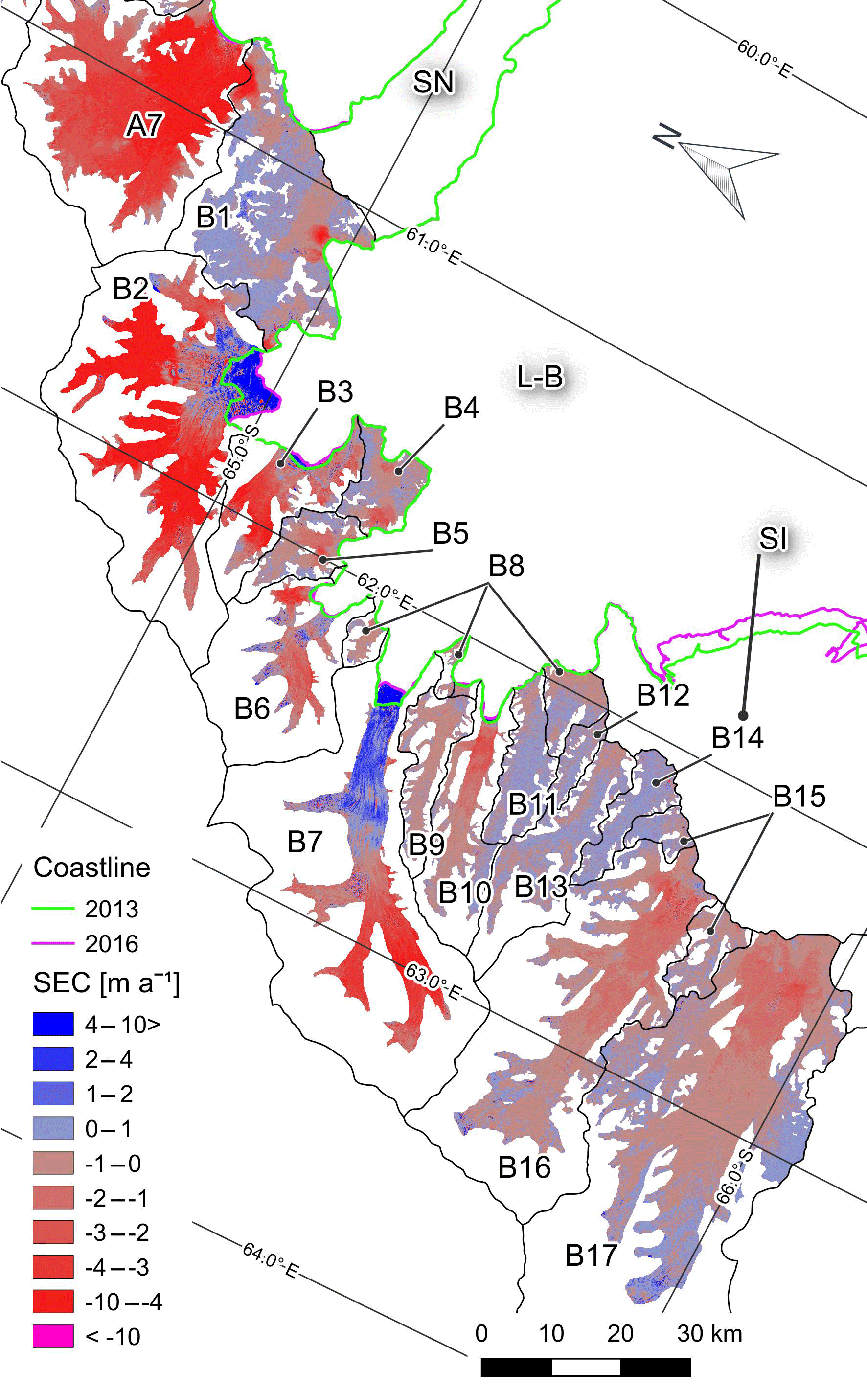
Figure 7 Map of surface elevation change (SEC, m a⁻¹) from June–July 2013 to July–August 2016 on glaciers of the Larsen B embayment (L-B). SN – Seal Nunataks. SI – Scar Inlet ice shelf.

Table 4 Rate of surface elevation change for areas by means of TDM DEM differencing from 2011 to 2013 for glacier basins of the Larsen B embayment. dh∕dt is the mean rate of elevation change in the area covered by the high-resolution map (Fig. 6). The basin area refers to ice front positions delineated in TanDEM-X images of 20 June and 1 July 2013. The rates of ice volume change (dV∕dt) and total mass balance (dM∕dt) refer to grounded ice.

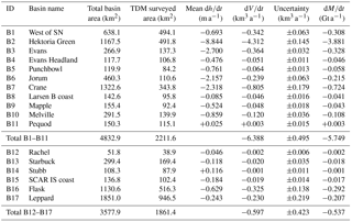
Table 5 Rate of surface elevation change for areas by means of TDM DEM differencing from 2013 to 2016 for glacier basins of the Larsen B embayment. dh∕dt is the mean rate of elevation change in the area covered by the high-resolution map (Fig. 7). The basin area refers to ice front positions delineated in TanDEM-X images of 27 June and 1 August 2016. The rates of ice volume change (dV∕dt) and total mass balance (dM∕dt) refer to grounded ice.

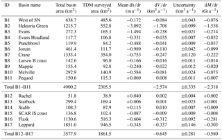
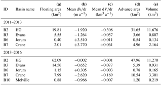
Table 6 (a) Area extent of floating ice in 2013 (top) and 2016 (bottom); (b) and (c) show the rate of surface elevation change and volume change in floating ice from 2011 to 2013 (top) and from 2013 to 2016 (bottom); (a–c) exclude the areas of frontal advance; (d) and (e) show the extent and volume of frontal advance areas.

4 Elevation change and mass balance of the Larsen B glaciers

4.1 Elevation change and mass balance by DEM differencing

The map of surface elevation change dh∕dt for the glacier basins discharging into the Larsen B embayment and Scar Inlet ice shelf is shown in Fig. 6 for the period May–June 2011 to June–July 2013 and in Fig. 7 for June–July 2013 to July–August 2016. The numbers on elevation change, volume change and mass balance, referring to grounded ice, are specified in Table 4 for 2011 to 2013 and in Table 5 for 2013 to 2016.

The SEC analysis shows large spatial and temporal differences in mass depletion between individual glaciers. The overall mass deficit of the Larsen B region is dominated by glaciers draining into the embayment where the ice shelf broke away in 2003 (basins B1 to B11). The annual mass balance of the glaciers draining into the Scar Inlet ice shelf (basins B12 to B17) was slightly negative in both periods: $B_{\text{n}}=-\mathrm{0.54}$ Gt a⁻¹ from 2011 to 2013 and $B_{\text{n}}=-\mathrm{0.58}$ Gt a⁻¹ from 2013 to 2016. The small glaciers (B12 to B15) were in a balanced state (Tables 4 and 5, Figs. 6 and 7). The mass deficit of the Flask and Leppard glaciers can be attributed to flow acceleration and increased ice export after break-up of the main section of the Larsen B ice shelf (Wuite et al., 2015).

In 2011 to 2013 the total annual net mass balance of basins B1 to B11 amounted to −5.75 Gt a⁻¹, with the mass deficit dominated by the Hektoria and Green (HG) glaciers ($B_{\text{n}}=-\mathrm{3.88}$ Gt a⁻¹), followed by Crane Glacier ($B_{\text{n}}=-\mathrm{0.72}$ Gt a⁻¹). The mass losses of the Evans and Jorum glaciers and of basin B1 (north-east of Hektoria Glacier) were also substantial, whereas the mass deficit of the other glaciers was modest. During the period 2013 to 2016 the annual mass deficit of the glacier ensemble was cut by more than half ($B_{\text{n}}=-\mathrm{2.32}$ Gt a⁻¹) compared to 2011 to 2013, with HG again dominating the loss ($B_{\text{n}}=-\mathrm{1.54}$ Gt a⁻¹). The decrease in mass depletion was also significant for other glaciers. For Crane Glacier the 2013 to 2016 losses ($B_{\text{n}}=-\mathrm{0.22}$ Gt a⁻¹) correspond to only 18 % of the estimated balance flux (Rott et al., 2011). This results in a large change after 2007 with $B_{\text{n}}=-\mathrm{3.87}$ Gt a⁻¹ (Wuite et al., 2015).

The decline of mass depletion coincided with a period of permanent cover by ice mélange and sea ice in the proglacial fjords and bays, starting in autumn/winter 2011. Several summers before, including the summer of 2010–2011, the sea ice in front of the glaciers drifted away and led to several weeks with open water. In the years thereafter the continuous sea ice cover obstructed the detachment of frontal ice and facilitated frontal advance. The maximum terminus advance was observed for HG glaciers, resulting in an increase in glacier area of 31.6 km² from 2011 to 2013 and 48.0 km² from 2013 to 2016 (Table 6).

Due to a significant decrease in ice thickness the floating area on Hektoria and Green glaciers increased significantly after 2011, covering an area of 19.8 km² inland of the 2011 ice front in June 2013 and an area of 62.1 km² inland of the 2013 ice front in June 2016 in addition to the frontal advance areas, where the ice was almost completely ungrounded. Areas of floating ice, covering several square kilometres in area, were observed on Evans Glacier and Crane Glacier. The areas of frontal advance showed a similar temporal trend, with an increase from 3.7 km² between 2011 and 2013 to 5.4 km² between 2013 and 2016 for Evans Glacier and 5.0 to 10.5 km² for Crane Glacier.

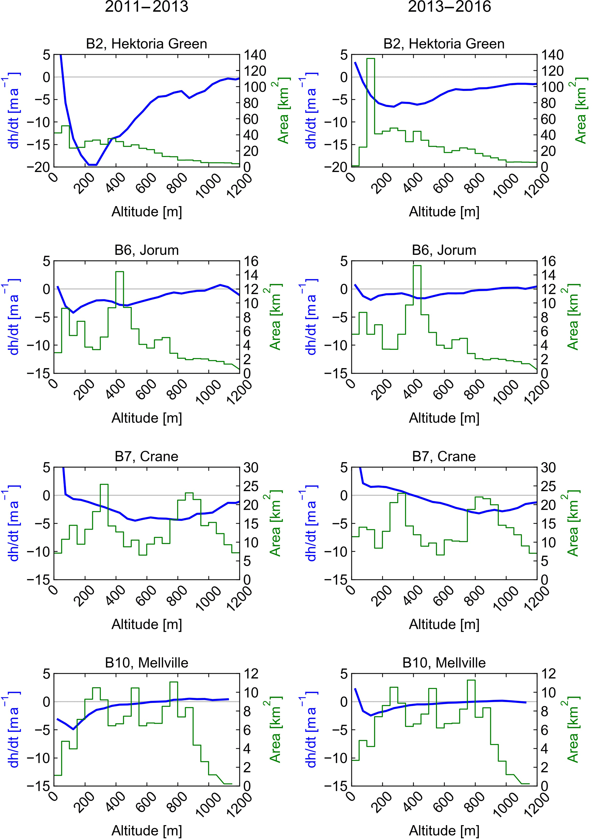
Figure 8 Rate of glacier surface elevation change dh∕dt (in m a⁻¹) from 2011 to 2013 and from 2013 to 2016 versus altitude in 50 m intervals for basins B2, B6, B7 and B10. Green line: hypsometry of surveyed glacier area in km².

Figure 8 shows the altitude dependence of elevation change (dh∕dt) for four basins with large mass deficits. The largest drawdown rate (19.5 m a⁻¹) was observed on HG glaciers in the elevation zone 200 to 300 m a.s.l. from 2011 to 2013, with substantial drawdown up to the 1000 m elevation zone. On Jorum Glacier the area affected by surface lowering extended up to 700 m elevation, with a maximum rate of 5 m a⁻¹. The drawdown pattern of Crane Glacier is different, with the zone of the largest 2011 to 2013 drawdown rates (4.5 m a⁻¹) commencing about 30 km inland of the front, extending across the elevation zone from 500 to 850 m a.s.l., and abating and shifting further upstream in 2013 to 2016. Scambos et al. (2011) observed an anomalous drawdown pattern on the Crane terminus during the first few years after ice shelf collapse, which was very likely associated with drainage of a subglacial lake.

4.2 Flow velocities, calving fluxes and mass balance using the mass budget method

Figure 9 shows maps of surface velocities in 2011 and 2016 and a map of the differences in velocity between October–November 1995 and 2016. Insets show differences in velocity between 2011 and 2016 for HG and Crane glaciers. Gaps in the 2011 TerraSAR-X/TanDEM-X velocity map are filled up with PALSAR data and in the 2016 map with Sentinel-1 data. The 1995 velocity map used as reference for pre-collapse conditions was derived from ERS 1-day interferometric repeat-pass data. The ERS data show very little difference between 1995 and 1999 flow velocities, suggesting that the glaciers were close to a balanced state during those years (Rott et al, 2011). In 2016 the velocities of the main glaciers were still higher than in 1995 but have slowed down significantly since 2011.

The temporal evolution of the Larsen B glaciers between 1995 and 2013 is described in detail by Wuite et al. (2015), showing velocity maps for 1995 and 2008–2012 and time series of velocities along central flow lines of eight glaciers between 1995 and 2013. Furthermore, here we report velocity changes since 2013 and provide details on velocities of HG and Crane glaciers in recent years, including a diagram of velocities across the flux gates on different dates (Fig. 10).

Figure 9 Magnitude of ice velocity (m d⁻¹) in 2011 (a) and 2016 (b) derived from TerraSAR-X and TanDEM-X data. Gaps in 2011 are filled with PALSAR data and in 2016 they are filled with Sentinel-1 data. (c) Map of velocity difference between 2016 and 1995. Insets: velocity difference between 2016 and 2011 for HG and Crane glaciers.

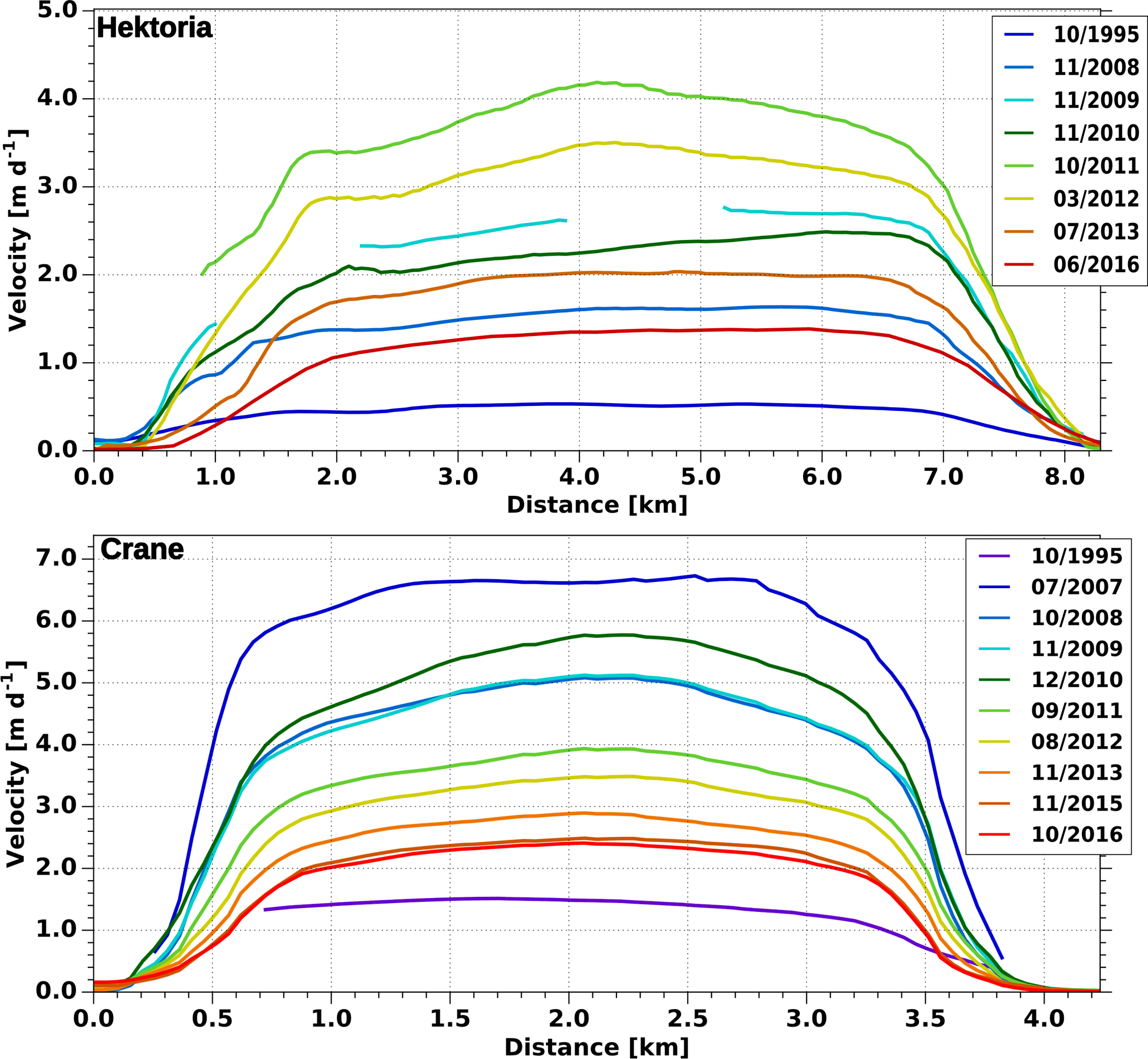
Figure 10 Surface velocity across the flux gate of Hektoria Glacier and Crane Glacier on different dates (month/year) between 1995 and 2016.

Flask and Leppard glaciers, discharging into the Scar Inlet ice shelf, and the small glaciers of the main Larsen B embayment (B4, B5, B8 to B11) showed only small variations in velocity after 2011, though in 2016 the velocities of these glaciers were still higher than during the pre-collapse period. The main glaciers were subject to significant slowdown. On Crane Glacier the velocity in the centre of the flux gate decreased from a value of 6.8 m d⁻¹ in July 2007 to 3.9 m d⁻¹ in September 2011, 2.9 m d⁻¹ in November 2013 and 2.4 m d⁻¹ in October 2016, which is still 50 % higher than the velocities in 1995 and 1999. Because of major glacier thinning, the cross section of the flux gate decreased significantly, so that the calving flux amounted in mid-2016 to 1.39 Gt a⁻¹, only 20 % larger than in 1995 to 1999. Since 2007 the drawdown rate of Crane Glacier has decreased steadily from a mass balance of −3.87 Gt a⁻¹ in June 2007 to −0.23 Gt a⁻¹ in November 2016. Also, on Jorum Glacier the calving velocity has decreased gradually since 2007; from 2013 to 2016 the glacier was close to a balanced state. In contrast, in 2011 to 2016 the velocity at the flux gate of Melville Glacier was only 5 % lower than in 2008, 2.6 times higher than the pre-collapse velocity reported by Rott et al. (2011). This agrees with the negative mass balance by TDM SEC analysis. However, the mass deficit is small in absolute terms because of the modest mass turnover.

The velocities of the Hektoria and Green glaciers have been subject to significant variation since 2002, associated with major frontal retreat but also with intermittent periods of frontal advance (Wuite et al., 2015). Between November 2008 and November 2009 the velocity in the centre of the Hektoria flux gate increased from 1.7 to 2.8 m d⁻¹, slowed down slightly during 2010 and accelerated again in 2011 to reach a value of 4.2 m d⁻¹ in November 2011, followed by deceleration to 3.5 m d⁻¹ in March 2012, 2.0 m d⁻¹ in July 2013 and 1.4 m d⁻¹ in June 2016 (Fig. 10). Similar deceleration was observed for Green Glacier, from 4.6 m d⁻¹ in November 2011 to 2.8 m d⁻¹ in July 2013 and 2.0 m d⁻¹ in June 2016.

The slowdown and frontal advance of the Larsen B calving glaciers coincided with a period of continuous cover by ice mélange and sea ice in the proglacial fjords after mid-2011, indicating significant impact of pre-frontal marine conditions on ice flow (Fig. S4). We tracked detached ice blocks close to glacier fronts to estimate the order of magnitude of motion. Typical values for 2013 to 2016 pre-frontal displacements are 6.1 km for Crane Glacier, 2.7 km for Melville Glacier, 2.5 km for Jorum Glacier and 0.9 km for Mapple Glacier. This corresponds to about twice the flux gate velocity for Crane Glacier and about 5 times for Melville Glacier. The 2013 to 2016 displacement of ice blocks in front of HG glaciers (4.5 km for Green, 3.9 km for Hektoria) exceeded only slightly the distance of frontal advance.

Table 7 Mean specific surface mass balance (b_n) in 2011–2016, annual surface mass balance (SMB) and calving flux (CF) in 2011–2013 and 2013–2016 and resulting mass balance (MB) in Gt a⁻¹ for Larsen B glaciers.

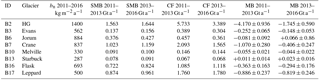
The comparisons of mass balance by MBM (Table 7) and SEC show good agreement overall as well as for most of the individual basins. The combined 2011 to 2013 annual mass balance of the five basins discharging into the main Larsen B embayment (B2, B3, B6, B7, B10) is −5.26 Gt a⁻¹ by TDM SEC and −5.63 Gt a⁻¹ by MBM, and for 2013 to 2016 −2.15 Gt a⁻¹ by TDM SEC and −2.28 Gt a⁻¹ by MBM. The SEC mass balance in this comparison also includes the volume change in the floating glacier sections (Table 6). Also, for Starbuck and Flask glaciers (B13, B16) the mass balance values of the two methods agree well. The only basin where the difference between the two methods exceeds the estimated uncertainty is Leppard Glacier (B17), where MBM ($B_{\text{n}}=-\mathrm{0.89}$ Gt a⁻¹ and $B_{\text{n}}=-\mathrm{0.82}$ Gt a⁻¹ for the two periods) shows higher losses than SEC ($B_{\text{n}}=-\mathrm{0.21}$ Gt a⁻¹ and $B_{\text{n}}=-\mathrm{0.30}$ Gt a⁻¹). The SEC retrievals of the basins B3, B7, B10, B13, B16, which show good agreement between SEC and MBM mass balance, are based on data from the same TDM track as B17. Therefore it can be concluded that the difference in MB of Leppard Glacier is probably due to a bias in SMB, in the cross section of the flux gate or in both. The specific surface mass balance (Table 7) for the adjoining Flask Glacier is 39 % higher than for Leppard Glacier.

5 Discussion

The main outlet glaciers in the northern sections of the Larsen ice shelf that disintegrated in 1995 (Prince Gustav Channel and Larsen A ice shelves, PGC–LA) and in 2002 (the main section of the Larsen B ice shelf) are still losing mass due to dynamic thinning. The losses are caused by accelerated ice flow tracing back to the reduction of back stress after ice shelf break-up, triggering dynamic instabilities (Rott et al., 2002, 2011; Scambos et al., 2004; Wuite et al., 2015; De Rydt et al., 2015; Royston and Gudmundsson, 2016).

On the outlet glaciers to PGC–LA (basins A1 to A7) the rate of mass depletion of grounded ice decreased by 40 % from the period 2011 to 2013 ($B_{\text{n}}=-\mathrm{3.98}\pm \mathrm{0.33}$ Gt a⁻¹) to the period 2013 to 2016 ($B_{\text{n}}=-\mathrm{2.38}\pm \mathrm{0.18}$ Gt a⁻¹). The mass deficit of the area was dominated by losses at Drygalski Glacier, with an annual mass balance of −2.18 Gt a⁻¹ in 2011 to 2013 and −1.72 Gt a⁻¹ in 2013 to 2016. Scambos et al. (2014) report a mass balance of −5.67 Gt a⁻¹ for glacier basins 21 to 25 for 2001 to 2008, corresponding approximately to our basins A1 to A7. On Drygalski Glacier the 2003 to 2008 annual mass balance (−2.39 Gt a⁻¹) by Scambos et al. (2014) was only 9 % lower than our estimate for 2011 to 2013. On the other glaciers of PGC and Larsen A embayment, the slowdown of calving velocities and decrease in calving fluxes during the last decade was more pronounced.

On the outlet glaciers to the Larsen B embayment (basins B1 to B11) the rate of mass depletion for grounded ice decreased by 60 % ($B_{\text{n}}=-\mathrm{5.75}$ ± 0.45 Gt a⁻¹ from 2011 to 2013, $B_{\text{n}}=-\mathrm{2.32}$ ± 0.25  Gt a⁻¹ from 2013 to 2016). Hektoria and Green glaciers accounted for the bulk of the mass deficit ($B_{\text{n}}=-\mathrm{3.88}$ Gt a⁻¹, $B_{\text{n}}=-\mathrm{1.54}$ Gt a⁻¹) in both periods. High drawdown rates were observed on HG glaciers from 2011 to 2013, with the maximum value (19.5 m a⁻¹) in the elevation zone from 200 to 300 m a.s.l. Our basins B1 to B11 correspond to the basins 26a and 27 to 31a of Scambos et al. (2014). Based on ICESat data spanning September 2003 to March 2008 and optical stereo image DEMs acquired between November 2001 to November 2006, Scambos et al. (2014) report an annual mass balance of −8.39 Gt a⁻¹ for these basins, excluding ice lost by frontal retreat. Our rate of mass loss for 2011 to 2013 amounts to 69 % of this value, and for 2013 to 2016 to 36 %, a similar percentage decrease in mass losses as for the PGC–LA basins. After ice shelf break-up in March 2002 the glacier flow accelerated rapidly, causing a large increase in calving fluxes during the first years after the Larsen B collapse, whereas on most glaciers the calving velocities slowed down significantly after 2007 (Scambos et al., 2004, 2011; Rott et al., 2011; Shuman et al., 2011; Wuite at al., 2015). An exception is basin B2 (HG glaciers) for which the 2011 to 2013 loss rate was 2 % higher than the value ($B_{\text{n}}=-\mathrm{3.82}$ Gt a⁻¹) reported by Scambos et al. (2014) for 2001 to 2008.

The drawdown pattern on the main glaciers shows high elevation loss rates for grounded ice shortly upstream of the glacier front or upstream of the floating glacier section, and abating loss rates towards higher elevations. This is the typical loss pattern for changes in the stress state at the downstream end of a glacier as a response to the loss of terminal floating ice (Hulbe et al., 2008). The elevation change pattern in recent years is different on Crane Glacier, where elevation decline and thinning migrated upglacier from 2011 to 2016, an indication for upstream-propagating disturbances (Pfeffer, 2007). Both patterns indicate that the glaciers are still far from a state of equilibrium, so dynamic thinning will continue for years.

We compiled surface motion and calving fluxes for the main glaciers of the study region and derived the surface mass balance from the output of the regional atmospheric climate model RACMO. These data enable individual components of the mass balance to be compared. Whereas the SMB between the periods 2011 to 2013 and 2013 to 2016 differed only by few percent, the calving fluxes decreased significantly due to slowdown of ice motion, confirming that the mass losses were of dynamic origin, an aftermath to changes in the stress regime after ice shelf collapse.

The terminus velocities on most glaciers are still higher than during the pre-collapse period. After rapid flow acceleration during the first years after ice shelf break-up there has been a general trend of deceleration afterwards, but with distinct differences in the temporal pattern between individual glaciers. Glaciers with broad calving fronts show larger temporal variability of velocities and calving fluxes than glaciers with a small width-to-length ratio. In the Larsen A embayment the Drygalski Glacier has been subject to major variations in flow velocity and calving flux during the last decade. In 2007 to 2009 the velocity in the centre of the flux gate varied between 5.5 and 6 m d⁻¹, increased to 8 m d⁻¹ in 2011 and 2012 and decreased to 6.0 m d⁻¹ in July 2016, which is still 4 times higher than the velocity in 1993. In the Larsen B embayment Hektoria and Green glaciers showed large temporal fluctuation in velocity and a general trend of frontal retreat, but also sporadic periods of frontal advance. A major intermittent acceleration event, starting in 2010, was responsible for a large mass deficit in 2011 to 2013.

Regarding the Scar Inlet ice shelf tributaries, the small glaciers (basin B12 to B15) were approximately in a balanced state, whereas Flask (B16) and Leppard (B17) glaciers showed a moderate mass deficit. The total mass balance of the Scar Inlet glaciers, based on TDM SEC analysis, was −0.54 ± 0.38 Gt a⁻¹ in 2011 to 2013 and −0.58 ± 0.38 Gt a⁻¹ in 2013 to 2016. As for the calving glaciers to the Larsen A and B embayments, the mass balance was less negative than during the period 2001 to 2008 ($B_{\text{n}}=-\mathrm{1.37}$ Gt a⁻¹) reported by Scambos et al. (2014).

The slowdown of flow velocities and decline in mass depletion between 2011 and 2016 coincided with periods of continuous coverage by ice mélange (a mixture of icebergs and bergy bits, held together by sea ice) and sea ice in the proglacial fjords and bays. After several summers with open water (excluding summer 2009–2010), a period of permanent coverage by ice mélange and sea ice commenced in the Larsen B embayment in winter 2011 and in PGC and Larsen A embayment in winter 2013. Observations and modelling of seasonal advance and retreat of calving fronts of Greenland outlet glaciers indicate that the buttressing pressure from rigid ice mélange is principally responsible for the seasonal variations (Walter et al., 2012; Todd and Christofferson, 2014; Amundson et al., 2016). Whereas for Greenland outlet glaciers ice mélange usually breaks up in spring, coinciding with ice flow acceleration and increased calving, the observations in the Larsen A and B embayments show persisting ice mélange and sea ice cover over multiyear periods. The cold water of the surface mixed layer in the western Weddell Sea favours sea ice formation and the persistence of sea ice during summer.

The sea ice cover impeded glacier calving, as apparent in frontal advance of several glaciers. Large frontal advance was observed for HG glaciers (∼ 3.2 km from 2011 to 2013 and ∼ 3.8 km from 2013 to 2016) and Crane Glacier (∼ 1.2 km from 2011 to 2013 and ∼ 2.5 km from 2013 to 2016). The front of Bombardier–Edgeworth glaciers advanced between 2013 and 2016 by 1.5 km and the front of Sjögren Glacier by 0.5 km. The continuous sea ice cover and restricted movement of ice calving from glaciers contrasts with the rapid movement of icebergs during the first few days after the Larsen A and B collapse, drifting away by up to 20 km per day due to strong downslope winds and local ocean currents (Rott et al., 1996; Rack and Rott 2004). For 2006 to 2015 a modest trend of atmospheric cooling was observed in the study region, in particular in summer (Turner et al., 2016; Oliva et al., 2017). However, this feature does not fully explain the striking difference in sea ice pattern and ice drift. Changes in regional atmospheric circulation patterns affecting the frequency and intensity of downslope foehn events play a main role in the presence of sea ice and the variability of melt patterns (Cape et al., 2015). Clem at al. (2016) show that the interannual variability of north-east peninsula temperatures is primarily sensitive to zonal wind anomalies and resultant leeside adiabatic warming. After 1999 changes in cyclonic conditions in the northern Weddell Sea resulted in a higher frequency of east to south-easterly winds, increasing the advection of sea ice towards the east coast of the Antarctic Peninsula (Turner at al., 2016). Superimposed on these regional patterns in atmospheric circulation are local differences in the relationship between melting and foehn winds causing a comparatively high degree of spatial variability in the melt pattern (Leeson et al., 2017). The break-up patterns of sea ice in summer 2017 show local differences. Sjögren fjord and the main section of the Larsen A embayment were clear of sea ice, whereas ice mélange and sea ice persisted in Larsen Inlet, the inlet in front of the DBE glaciers and in the Larsen B embayment.

6 Conclusions

The analysis of surface elevation change by DEM differencing over the periods 2011 to 2013 and 2013 to 2016 shows continuing drawdown and major losses in ice mass for outlet glaciers to Prince Gustav Channel and the Larsen A and B embayments. During the observation period 2011 to 2016 there was a general trend of decreasing mass depletion, induced by slowdown of calving velocities resulting in reduced calving fluxes. For several glaciers frontal advance was observed in spite of ongoing elevation losses upstream. The mass balance numbers for the glaciers north of Seal Nunataks are −3.98 ± 0.33 Gt a⁻¹ from 2011 to 2013 and −2.38 ± 0.18 Gt a⁻¹ from 2013 to 2016. The corresponding numbers for glaciers calving into the Larsen B embayment for the two periods are −5.75 ± 0.45 and −2.32 ± 0.25 Gt a⁻¹. For the glacier discharge into the Scar Inlet ice shelf the losses were modest.

The period of decreasing flow velocities and frontal advance coincides with several years in which ice mélange and sea ice cover persisted in proglacial fjords during summer. Considering the ongoing mass depletion of the main glaciers and the increase in ungrounded glacier area due to thinning, we expect a recurrence of periods with frontal retreat and increasing calving fluxes, in particular for those glaciers that showed major temporal variations in ice flow during the last several years. In the Larsen A embayment large fluctuations in velocity were observed for Drygalski Glacier and in the Larsen B embayment for the Hektoria and Green glaciers. These are the glaciers with the main share in the overall mass loss of the region: Drygalski Glacier contributed 61 % to the 2011 to 2016 mass deficit of the Larsen A/PGC outlet glaciers, and HG glaciers accounted for 67 % of the mass deficit of the Larsen B glaciers. On HG glaciers the ice flow accelerated significantly in 2010–2011, triggering elevation losses up to 19.5 m a⁻¹ on the lower terminus during the period 2011 to 2013. HG glaciers have a joint broad calving front and the frontal sections are ungrounded, thus are more vulnerable to changes in atmospheric and oceanic boundary conditions than glaciers that are confined in narrow valleys.

Complementary to DEM differencing, we applied the mass budget method to derive the mass balance of the main glaciers. The mass balance numbers of these two independent methods show good agreement, affirming the soundness of the reported results. The agreement also backs up the reliability of the RACMO SMB data. A strong indicator of the high quality of the TDM SEC products is the good agreement with 2011–2016 SEC data measured by the airborne laser scanner of NASA IceBridge. Both data sets were independently processed. The agreement indicates that SAR signal penetration does not affect the retrieval of surface elevation change on glaciers by InSAR DEM differencing if repeat observation data are acquired over snow/ice media with stable backscatter properties under the same observation geometry.