the Creative Commons Attribution 4.0 License.
the Creative Commons Attribution 4.0 License.
 | 10 Apr 2018
Thermodynamic and dynamic ice thickness contributions in the Canadian Arctic Archipelago in NEMO-LIM2 numerical simulations
Jingfan Sun
Ting On Chan
Paul G. Myers
Sea ice thickness evolution within the Canadian Arctic Archipelago (CAA) is of great interest to science, as well as local communities and their economy. In this study, based on the NEMO numerical framework including the LIM2 sea ice module, simulations at both 1∕4 and horizontal resolution were conducted from 2002 to 2016. The model captures well the general spatial distribution of ice thickness in the CAA region, with very thick sea ice (∼ 4 m and thicker) in the northern CAA, thick sea ice (2.5 to 3 m) in the west-central Parry Channel and M'Clintock Channel, and thin (<2 m) ice (in winter months) on the east side of CAA (e.g., eastern Parry Channel, Baffin Island coast) and in the channels in southern areas. Even though the configurations still have resolution limitations in resolving the exact observation sites, simulated ice thickness compares reasonably (seasonal cycle and amplitudes) with weekly Environment and Climate Change Canada (ECCC) New Ice Thickness Program data at first-year landfast ice sites except at the northern sites with high concentration of old ice. At 1∕4 to scale, model resolution does not play a significant role in the sea ice simulation except to improve local dynamics because of better coastline representation. Sea ice growth is decomposed into thermodynamic and dynamic (including all non-thermodynamic processes in the model) contributions to study the ice thickness evolution. Relatively smaller thermodynamic contribution to ice growth between December and the following April is found in the thick and very thick ice regions, with larger contributions in the thin ice-covered region. No significant trend in winter maximum ice volume is found in the northern CAA and Baffin Bay while a decline (r2 ≈ 0.6, p < 0.01) is simulated in Parry Channel region. The two main contributors (thermodynamic growth and lateral transport) have high interannual variabilities which largely balance each other, so that maximum ice volume can vary interannually by ±12 % in the northern CAA, ±15 % in Parry Channel, and ±9 % in Baffin Bay. Further quantitative evaluation is required.
- Article
(9506 KB) - Full-text XML
- BibTeX
- EndNote


The Canadian Arctic Archipelago (CAA), the complex network of shallow-water channels adjacent to the Arctic ice pack, has been a scientific research hot spot for a long time. Scientifically, it is an important pathway delivering cold, fresh Arctic water downstream (Dickson et al., 2007; Melling et al., 2008; Peterson et al., 2012; Prinsenberg and Hamilton, 2005) that eventually feeds the North Atlantic Ocean, where the water mass formation and ocean dynamics play a key role in the large-scale meridional overturning circulation and global climate variability (Hátún et al., 2005; Marshall et al., 2001; Rhein et al., 2011; Vellinga and Wood, 2002). Economically, shipping through the CAA, via the Northwest Passage (NWP), is of particular interest to commercial transport between Europe and Asia because of the great distance savings compared to the current route through the Panama Canal (Howell et al., 2008; Pizzolato et al., 2014, 2016). This has been a hot topic considering that northern hemispheric sea ice cover has been declining dramatically (Comiso et al., 2008; Parkinson and Cavalieri, 2008; Parkinson and Comiso, 2013; Parkinson et al., 1999; Serreze et al., 2007; Stroeve et al., 2008), especially after 2007. Besides the harsh weather and other safety issues (e.g., icebergs), the biggest concern for using the NWP is still the condition of sea ice, especially high concentrations of thick multiyear ice (MYI) (Haas and Howell, 2015; Howell et al., 2008; Melling, 2002).
Lietaer et al. (2008) estimated about 10 % of the total northern hemispheric sea ice volume is stored within the CAA. Sea ice within the CAA region is a combination of both first-year ice (FYI) and MYI. MYI is both locally formed and imported from the Arctic Ocean and is normally located in the central-west Parry Channel and northern CAA (Howell et al., 2008, 2013; Melling, 2002). Since the late 1970s, the ice-free season has extended by about 1 week per decade (Howell et al., 2009), with a statistically significant decrease of 8.7 % per decade in the September FYI cover. Reduction in the September MYI cover is also found to be −6.4 % per decade until 2008 (Howell et al., 2009). But this trend was not “yet statistically significant” due to the inflow of MYI from the Arctic Ocean mainly via the Queen Elizabeth Islands (QEI) gates in August to September (Howell et al., 2009). With extended data in recent years (until 2016), Mudryk et al. (2017) showed that the summer MYI decline rate has almost doubled. Even though the Arctic Ocean ice pack also extends to the CAA region through M'Clure Strait, the net sea ice flux is small and usually leads to an outflow from the CAA (Agnew et al., 2008; Howell et al., 2013; Kwok, 2006).
Although there is increasing demand for sea ice thickness information within this region, there are still very limited records available (Haas and Howell, 2015). Melling (2002) analyzed drill-hole data measured in winters during 1971–1980 within the Sverdrup Basin (the marine area between Parry Channel and QEI gates, see Fig. 1) and found that sea ice in this region is landfast (100 % concentration without motion) for more than half of the year (from October–November to late July) with a mean late winter thickness of 3.4 m. Sub-regional means of the ice thickness can reach 5.5 m, but very thick multiyear ice was found to be less common, which is likely due to the melting caused by tidally enhanced oceanic heat flux in this region (Melling, 2002). The seasonal transport of the old ice from the Sverdrup Basin down to the south was known to occur (Bailey, 1957), which helps to create another major region with severe MYI conditions in the CAA, the central Parry Channel and M'Clintock Channel (see Fig. 1 for the location). Based on two airborne electromagnetic (AEM) ice thickness surveys conducted in May 2011 and April 2015, Haas and Howell (2015) estimated the ice thickness to be 2 to 3 m in this region with MYI thicker than 3 m on average. This supports the general spatial distribution of ice thickness within the CAA, thicker in the north and relatively thinner in the south.
Observations were not only limited in time but also in spatial coverage; thus, numerical simulations are required to better understand the ice distribution and variability in the CAA (Dumas et al., 2006; Hu and Myers, 2014; Sou and Flato, 2009). Dumas et al. (2006) evaluated the simulated ice thickness at CAA meteorological stations but with a uncoupled one-dimensional (1-D) sea ice model (Flato and Brown, 1996). The variability and trends of landfast ice thickness within the CAA were systematically studied by a recent paper from Howell et al. (2016) based on historical records at observed sites (Cambridge Bay, Resolute, Eureka, and Alert) and numerical model simulations over the 1957–2014 period. They found statistically significant thinning at the sites except at Resolute, and the detrended interannual variability is high (negative) correlated with snow depth due to the insulating effect of the snow (Brown and Cote, 1992). Although some of the numerical simulations used in Howell et al. (2016) produced a reasonable seasonal cycle generally, these simulations overestimated ice thickness and did not do a good job in capturing the trend. In addition, the lack of horizontal resolution in these models were also pointed out in Howell et al. (2016).
In this paper, we focus on the simulated CAA sea ice thickness over recent years (2002–2016), focussing on (1) the evaluation of the skill of a numerical model in simulating sea ice thickness compared with the landfast ice thickness at several sites in the CAA and (2) the relative importance of thermodynamic and dynamic processes in the simulated sea ice seasonal and interannual changes in the CAA. This paper starts with a brief description of the numerical simulations and observational data used in this study. Then the evaluation of simulated ice thickness in the CAA region is presented in Sect. 3.1. The spatial distribution and temporal evolution (at selected sites) of thermodynamic and dynamic ice thickness contributions are studied in Sect. 3.2. Ice volume budgets in the northern CAA, Parry Channel, and Baffin Bay are discussed in Sect. 3.3. Concluding remarks and discussions are given in Sect. 4.
2.1 Numerical model setup
In this study, the coupled ocean sea ice model, the Nucleus for European Modelling of the Ocean (NEMO, available at https://www.nemo-ocean.eu) version 3.4 (Madec and the NEMO team, 2008), is utilized to conduct the numerical simulations. The model domain covers the Arctic and the Northern Hemisphere Atlantic (ANHA) with two open boundaries, one close to Bering Strait in the Pacific Ocean and the other one at 20∘ S across the Atlantic Ocean (Fig. 1, inset). The model mesh is extracted from the global tripolar grid, ORCA (Drakkar Group, 2007), with two different horizontal resolutions, 1∕4∘ (hereafter ANHA4) and 1∕12∘ (hereafter ANHA12). The highest horizontal resolution is ∼ 2 km for ANHA12 and ∼ 6 km for ANHA4 in Coronation Gulf–Dease Strait region, which is near the artificial pole over northern Canada (Fig. 1), and the lowest resolution is ∼ 9 km for ANHA12 and ∼ 28 km for ANHA4 at the Equator. In the vertical, there are 50 geopotential levels with high resolution focused in the upper ocean. Layer thickness smoothly transitions from ∼ 1 m at surface (22 levels for the top 100 m) to 458 m at the last level.
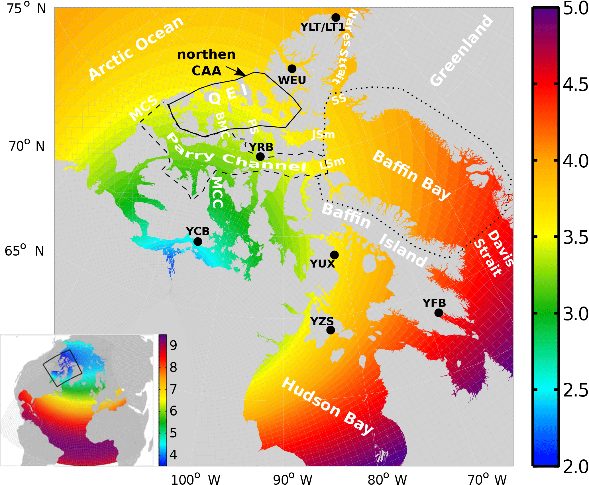
Figure 1ANHA12 (inset) model mesh (every 10th grid point) and horizontal resolution (colours, unit: kilometres) in the Canadian Arctic Archipelago (QEI: Queen Elizabeth Islands; MCS: M'Clure Strait; MCC: M'Clintock Channel; BMC: Byam Martin Channel; PS: Penny Strait; JSm: Jones Sound Mouth; LSm: Lancaster Sound Mouth; SS: Smith Sound) and Hudson Bay region (thick black box highlighted in the inset. Note the colour scale is different from that used in the inset). Ice thickness observation sites (YZS: Coral Harbour, YUX: Hall Beach; YFB: Iqaluit; YCB: Cambridge Bay; YRB: Resolute; WEU: Eureka; YLT: Alert; LT1: Alert LT1) are shown with black circles on the map. Detailed location information of observation sites is available in Table 2.
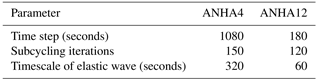
The sea ice module used here is the Louvain-la-Neuve Ice Model Version 2 (LIM2) with an elastic–viscous–plastic (EVP) rheology (Hunke and Dukowicz, 1997), including both thermodynamic and dynamic components (Fichefet and Maqueda, 1997). It is based on a three-layer (one snow layer and two ice layers of equal thickness) model proposed by Semtner Jr. (1976) with two ice thickness categories (mean thickness and open water). The sea ice module is coupled to the ocean module every model step. The elastic timescale is tuned small enough to damp the elastic wave in the EVP approach (see Table 1), based on the discussions in Hunke and Dukowicz (1997). Note that recent studies (Bouillon et al., 2013; Lemieux et al., 2012; Williams et al., 2017) showed that more iterations are needed to reach a viscous–plastic solution. Without doing that, the divergence field will be affected, i.e., being noisy (Frédéric Dupont, personal communication, 2017). Thus, to what degree it will impact the final averaged ice thickness will vary in space. Such an investigation in the CAA is beyond the scope of this study. A no-slip boundary condition is applied for sea ice in the simulations, which means the ice can have zero velocity along the coast. However, it should be noted that the sea ice module used in this study does not include a representation of landfast ice (Lemieux et al., 2016), which may negatively impact the sea ice simulation where landfast ice exists.
Two simulations, ANHA4-CGRF and ANHA12-CGRF, are integrated from 1 January 2002 to 31 December 2016. The initial conditions, including three-dimensional (3-D) ocean fields (temperature, salinity, zonal velocity, and meridional velocity) as well as two-dimensional (2-D) sea surface height and sea ice fields (concentration and thickness), are taken from the Global Ocean Reanalysis and Simulations (GLORYS2v3) produced by Mercator Ocean (Masina et al., 2017). Open boundary conditions (temperature, salinity, and horizontal ocean velocities) are derived from the monthly GLORYS2v3 product as well. At the surface, the model is driven with high temporal (hourly) and spatial resolution (33 km) atmospheric forcing data provided by Canadian Meteorological Centre (CMC) Global Deterministic Prediction System (GDPS) reforecasts (CGRF) dataset (Smith et al., 2014), including 10 m wind, 2 m air temperature and humidity, downwelling and longwave radiation flux, and total precipitation. These forcing fields are linearly interpolated onto the model grid. Interannual monthly river discharge data from Dai et al. (2009) as well as Greenland meltwater (5 km × 5 km) provided by Bamber et al. (2012) are carefully (volume conserved) remapped onto the model grid.
With the same setting as ANHA4-CGRF but driven with the interannual atmospheric forcings from the Coordinated Ocean-ice Reference Experiments version 2 (CORE-II) (Large and Yeager, 2009), another ANHA4 simulation, ANHA4-CORE, integrated from 1 January 2002 to 31 December 2009, is also conducted to study the sensitivity of the sea ice simulation to the atmospheric forcings. The CORE-II provides fields at various temporal resolutions: (a) 6-hourly 10 m surface wind, 10 m air temperature and specific humidity; (b) daily downward longwave and shortwave radiation; and (c) monthly total precipitation and snowfall. No temperature or salinity restoring is applied in any of the simulations used in this study. Without such constraints the model evolves freely in time to help understand better the limitations of the physical processes represented by the model.
2.2 Environment and Climate Change Canada New Arctic Ice Thickness Program
To evaluate the performance of the model in terms of ice thickness, simulated ice thickness is compared to the observed landfast ice data from Environment and Climate Change Canada (ECCC) New Ice Thickness Program (hereafter ECCC thickness). The new ECCC thickness program, the second stage of the Original Ice Thickness Program Collection used in Dumas et al. (2006), started in the fall of 2002, and continued to the present at only 11 stations (including sites on lakes). Measurements were conducted weekly at approximately the same location close to shore between freeze-up and break-up (when the ice was safe to walk on) with a special auger kit or a hot wire ice thickness gauge. Note the measurement represents the immobile level first-year (seasonal) ice of uniform thickness that forms close to shore; however, simulated ice thickness, e.g., due to resolution, generally is an estimation of the mean state of different types of ice (e.g., first-year level ice, young ice, and old ice).
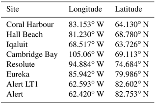
Data are made available to the public by Environment and Climate Change Canada under the Open Government License (Canada) at http://open.canada.ca/data/en/dataset (last access: 4 April 2017). Eight coastal sites – Coral Harbour, Hall Beach, Iqaluit, Cambridge Bay, Resolute, Eureka, Alert, and Alert LT1 – were used in this study. The remaining three sites are on lakes (not included in our simulations). The detailed location information of each site can be found in Fig. 1 and Table 2.
Table 2ECCC ice thickness station locations (only sites used in this study).
Unlike the 1-D model used in Dumas et al. (2006), which can be applied at the exact location where the measurements were carried out, 3-D models usually have horizontal resolution issues in resolving the observation sites, even with the high-resolution ANHA12 configuration used in this study. Interpolation is needed to do the comparison between simulated fields and observations. This is also mentioned in Howell et al. (2016). To interpolate simulated fields onto the nearest water point (xk,yk) of each observation site (xobs,yobs), we utilized a modified inverse distance weighting method (Eq. 1) proposed by Renka (1988):
where Rw is the influence radius about point (xk,yk), dk is the distance from point (xk,yk) to each neighbouring point (xi,yi), fi is the inverse distance function, wi is the weight function on each neighbouring point (xi,yi), N is the number of neighbouring points within Rw, Qi is variable value on each neighbouring point, and Qtarget is the final result. In practice, nine neighbouring points, including point (xk,yk), were considered in the calculation. As Rw is set to the maximum value of dk and land points should be excluded, eventually up to eight effective points are used in our interpolation process.
In this section, first the ice thickness reproduction ability within the CAA of the NEMO-LIM2 configurations used in this study is examined via comparisons with the ECCC thickness. Second, the detailed thermodynamic and dynamic ice thickness changes, both the spatial distribution and temporal evolution at selected sites (Cambridge Bay and Resolute), based on the simulation outputs will be presented. Ice volume balance, focusing on the thermodynamics contribution and lateral transport, in the northern CAA, Parry Channel, and Baffin Bay will also be included at the end.
3.1 Ice thickness comparison
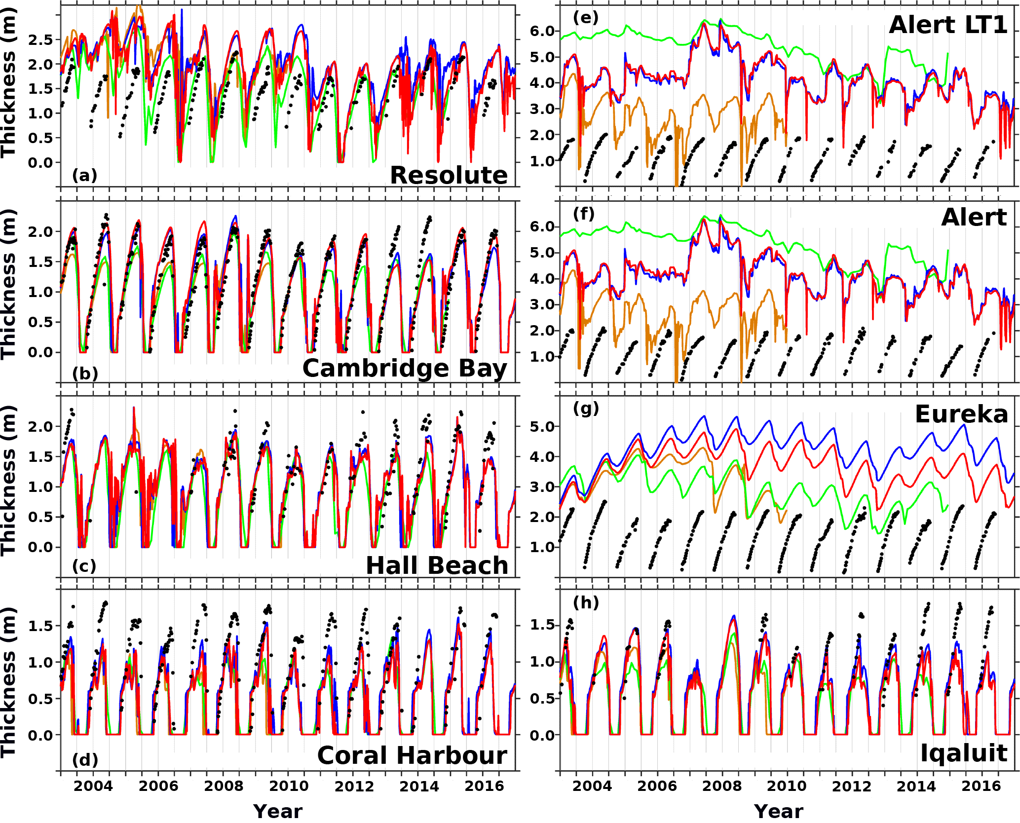
Figure 2Simulated ice thickness at each selected ECCC thickness site (Fig. 1 and Table 2, unit: metres) from January 2003 to December 2016 (orange: ANHA4-CORE simulation; green: GLORYS2v3 product; blue: ANHA4-CGRF simulation; red: ANHA12-CGRF simulation) against weekly ECCC observations (black dots). Note the GLORYS2v3 product is a monthly mean field while the rest of the simulations use 5-day averages. Different y axis scales are used.
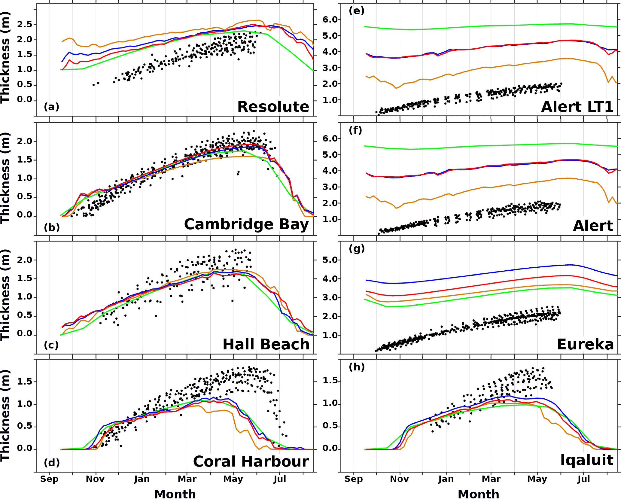
Figure 3Similar to Fig. 2 but for ice thickness seasonal cycle (starting from 17 September to the next 12 September, averaged over 2003 to 2016; ANHA4-CORE ends by 2009). Note observations are not averaged over time because the sampling time is different from year to year).
Figure 2 shows the ice thickness comparison with observations. In general, both ANHA4-CGRF (blue lines) and ANHA12-CGRF (red lines) simulations produce similar seasonal and interannual variations in ice thickness, which compare reasonably well at some sites (i.e., Cambridge Bay, Coral Harbour, Hall Beach, Resolute, and Iqaluit) but not at the others (Eureka, Alert, and Alert LT1). The sites where the model produced much thicker ice are likely where significant concentrations of old ice exists (CIS, 2011). Although the observations are missing in the sea ice melting season, an asymmetric seasonal cycle (a shorter faster melting period follows a relatively longer slow growth period) is evidenced by the available data and reproduced by the simulations. This is clearly shown in the ice thickness seasonal cycle plot (Fig. 3). Taking account of the model resolution, the interpolated simulated ice thickness reflects the variability some distance off the coast rather than the exact observation locations. The geographic location differences, which are also related to model resolution, could also lead to discrepancies in the comparisons here. Thus, if the model can capture the seasonal cycle (e.g., multiple data points in both ice growth and melting seasons), the model is likely capable of simulating the process.
At Iqaluit, the model did a good job in most years during the initial ice growth period but failed to catch the thick sea ice in the next April and May (Fig. 3), particularly in 2014, 2015, and 2016 (Fig. 2h). This could be a local atmospheric forcing field bias or a model resolution issue, i.e., the measurements captured very localized extremes beyond the ability of model to resolve. Similar behaviour happens at Coral Harbour and Hall Beach (Fig. 2c and d). Further investigation is needed.
At Eureka, Alert, and Alert LT1 sites (Figs. 2 and 3e, f, and g), there are clear differences between the simulated ice thickness and the observations (∼ 2 m at Alert/Alert LT1 and ∼ 1 m at Eureka). Note that neither ANHA4 nor ANHA12 has the capability to resolve the difference between Alert and Alert LT1; thus, the same simulated values are shown on the figure for both sites. The differences between simulations and observations could be an initial value problem, particularly at Eureka (Fig. 2g). However, given high concentrations of old ice are at these sites, observations represent the immobile level first-year ice only. Thus, the model and the observations may not be representing the same type of ice. At Alert and Alert LT1, both ANHA4-CGRF (blue line) and ANHA12-CGRF (red line) show similar interannual trends to that in GLORYS2v3 (which extends back to 1993, green line), meaning it is likely a pure initial value problem rather than the model equilibrium issue mentioned in Howell et al. (2016). In addition, the seasonal cycle is not clear in the GLORYS2v3 product. The issue is also present in some years, i.e., 2005–2007, in the ANHA4-CGRF and ANHA12-CGRF simulations. ANHA4-CORE (orange line) is generally improved compared with the observations in both the amplitude and seasonal cycle. However, this improvement was achieved by accident and is related to a snow depth issue in this simulation. The snowfall data from CORE-II have a monthly resolution, which is possibly too coarse temporally (Hakase Hayashida, personal communication, 2017). This leads the snow depth to drop to close to zero quickly during the first year of the simulation but not in the CGRF simulations with hourly snowfall. Thus, it does not indicate that CORE-II forcing is performing better than other atmospheric forcing datasets in this region. The equilibrium issue, i.e., ice thickness keeping increasing, might happen at Eureka in our simulations with either CGRF or CORE-II forcing. The upward trend over 2005 to 2007 is also present in the observations but is missing in the GLORYS2v3 although GLORYS2v3 has a small thickness (which is likely due to data assimilation in GLORYS2v3 or an atmospheric forcing issue in 2005). Its trend does not reflect the real change or variability.
At Cambridge Bay, simulations (red and blue lines in Fig. 2b) with CGRF forcing show very good agreement with the observations except during the winters of 2013 and 2014. Considering the horizontal resolution of our simulations is not capable of resolving the inner bay at Cambridge Bay, the match in ice thickness between the simulation and observations indicates the variation of ice thickness within the inner Bay might be small. Both ANHA4-CORE and GLORYS2v3 simulations underestimated the maximum values in winters by ∼ 0.5 m. This indicates CGRF forcing might provide more realistic surface inputs in this region.
At Resolute, it is more complicated (Fig. 2a). Prior to the significant sea ice melting in 2007, none of the simulations show ice-free conditions in this region in summer. GLORYS2v3 shows relatively thinner ice in summer months but it is still 0.5 to 1.5 m thick. It could be the initial value problem. However, high-frequently variations even in winter in the ANHA simulations suggest that the ice growth process is not dominated by a smoothly changing physical process (e.g., air temperature). Thus, it is likely due to another physical process such as advection from surrounding areas. This will be discussed more in the following section. Post-2007, the seasonal cycle in the sea ice field is more distinct, although ice-free summer conditions do not happen every year. After 2010, simulations produce winter sea ice thickness much closer to the observations.
3.2 Thermodynamic and dynamic ice thickness change
In the real world, both the thermodynamic and dynamic ice thickness processes are coupled together (occurring at the same time). However, with the assistance of numerical model, the two processes can be decoupled (shown in Eq. 2) to better understand the relative importance of each process.
where ΔHtotal is the total ice thickness change over a specific time interval, ΔHthermal is the ice thickness change due to vertical heat fluxes (through the atmosphere–ice–ocean interfaces), and ΔHdynamic is the ice thickness change due to dynamic processes. In practice, a simple approach is utilized to compute the two terms on the right side. ΔHthermal is calculated based on the model thermal ice production. ΔHdynamic is taken as the residual from the ΔHtotal.
3.2.1 Spatial distribution
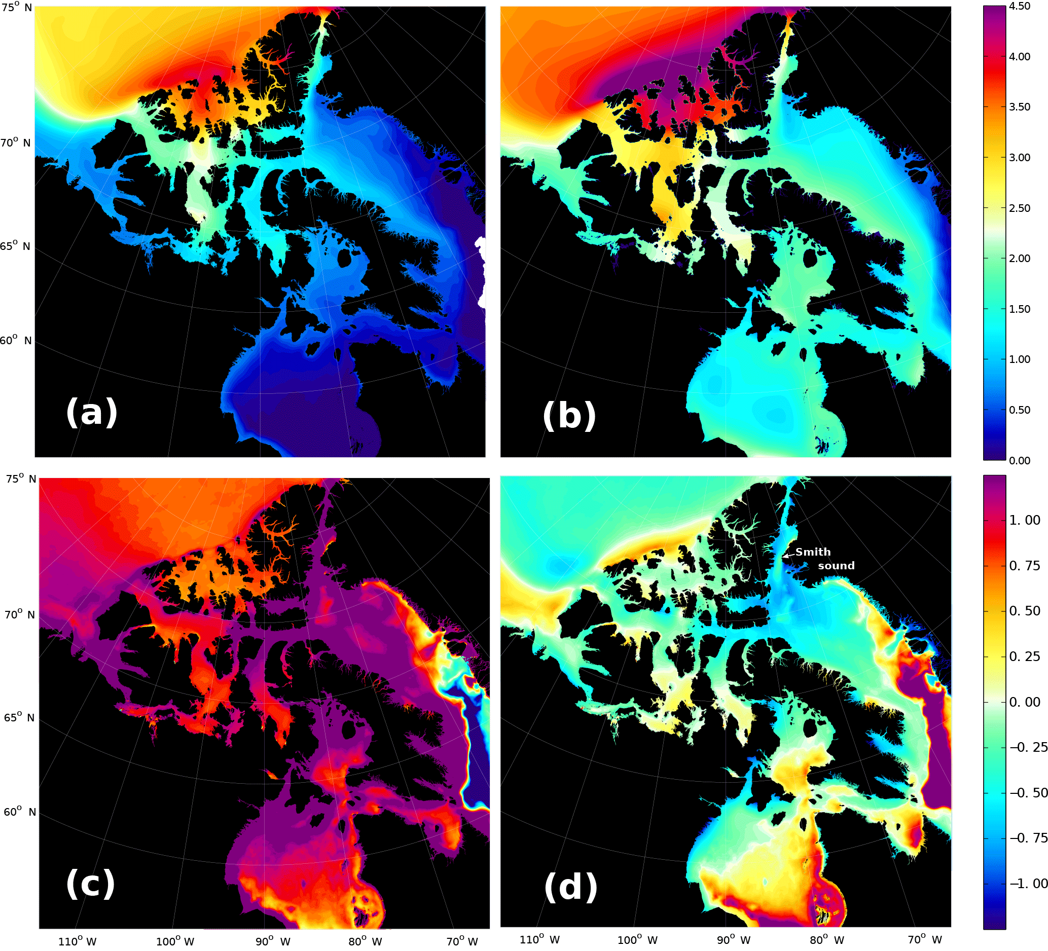
Figure 4Upper panel shows the thickness (unit: metres) averaged over 2003–2016 at the beginning of December (a) and at end of April (b). Lower panel shows the thermodynamics component (c) and dynamic component (d) ice thickness contribution (unit: metres) between December (a) and the following April (b) averaged over 2003–2015. ANHA12-CGRF simulation is used here.
Here we focus on ice growth process between December and April of the following year. Figure 4a and b show the simulated ice thickness in ANHA12 at the beginning of December and at the end of April, respectively. Geographically, at the end of April, very thick sea ice is located in the northern CAA (∼ 4 m by the end of April) with regional maximum (> 4.5 m) at the openings to the Arctic Ocean. This is consistent with the ICESat and Cryosat-2 estimations (Kwok and Cunningham, 2015; Laxon et al., 2013; Tilling et al., 2015). Less thick sea ice covers western, and central Parry Channel (just to the west of the site Resolute) and M'Clintock Channel with a thickness of 2.5 to 3 m. These values are similar to previous observations from airborne electromagnetic surveys (Haas and Howell, 2015) and satellite (Tilling et al., 2018). Relatively thin ice (<2 m) is mainly in the southern CAA, eastern Parry Channel, coast of Baffin Island, and within Hudson Bay. Invasion of the Arctic Ocean ice pack through the northern CAA openings and the advection from there into central Parry Channel are clearly shown in the figures, consistent with previous studies Haas and Howell (2015); Howell et al. (2008); Melling (2002).
During the winter, sea ice grows everywhere in the CAA regions due to the thermodynamic cooling (Fig. 4c). But the total increase over the winter is not evenly distributed in space, and ice growth is not largest in the north. Large thermodynamic ice growth is seen in the eastern CAA (eastern Parry Channel, Nares Strait, Baffin Island coast, and western Hudson Bay), Amundsen Bay, and many coastal regions (e.g., western coast of Banks Island, northern coast of western Parry Channel). Regions covered by thick sea ice (i.e., northern CAA, west-central Parry Channel, and M'Clintock Channel) show less thermodynamic ice growth over the winter. This is particularly true in the northern CAA, likely due to the existence of already thick ice reducing the heat exchange between the ocean and atmosphere.
The dynamic contribution to sea ice thickness is mainly negative (reduces local ice thickness) within the CAA (Fig. 4d). Large positive values (0.4 to 0.7 m) are shown along the Arctic Ocean coast off the CAA and within the Beaufort Sea. This is consistent with known sea ice convergence or strong advection of thick ice from upstream regions (Kwok, 2015; Maslanik et al., 2011). Within the northern CAA, west-central Parry Channel, and M'Clintock Channel, there is ∼ 0.25 m thick ice loss locally due to the dynamics. Note the positive values occurring in the south of M'Clintock Channel, suggesting a net convergence there which contributes to the local ice thickening in winter. In the eastern CAA (e.g., eastern Parry Channel, Nares Strait, and northwest corner of Baffin Bay), there are large negative dynamic thickness contributions, implying strong ice advection.
Although the North Water (NOW) Polynya (Dunbar, 1969; Melling et al., 2001) region is still ice covered by the end of April (Fig. 4b), the spatial distribution of negative dynamic ice thickness (which helps to remove local ice) captures the shape of NOW Polynya well. Weaker advection of sea ice at Smith Sound and to its south, which is likely to be caused by ice jamming, is also simulated by the model.
3.2.2 Seasonal cycle at Cambridge Bay and Resolute
Two sites, Cambridge Bay and Resolute, were selected to further study the seasonal cycle of the thermodynamic and dynamic ice thickness changes.
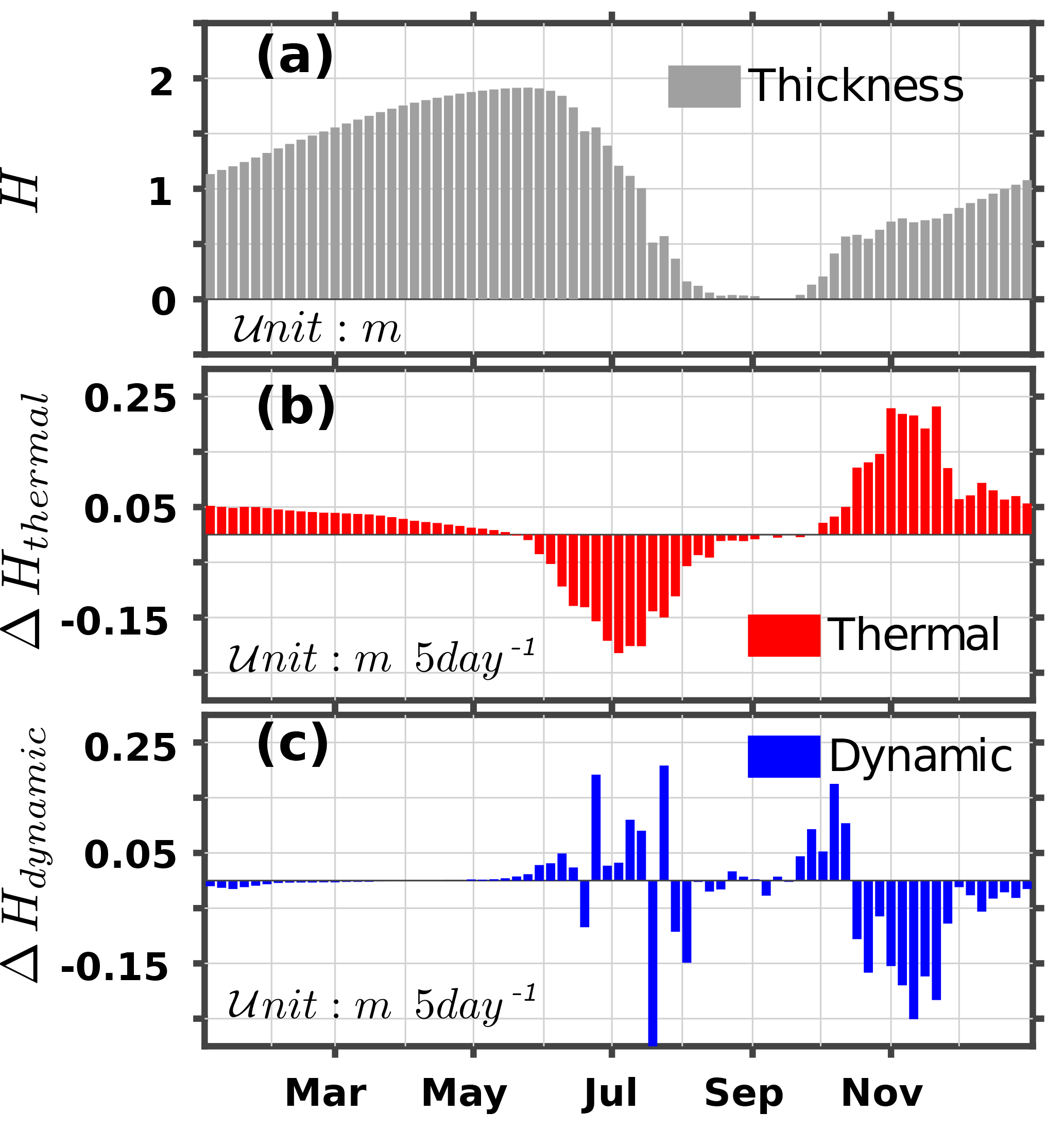
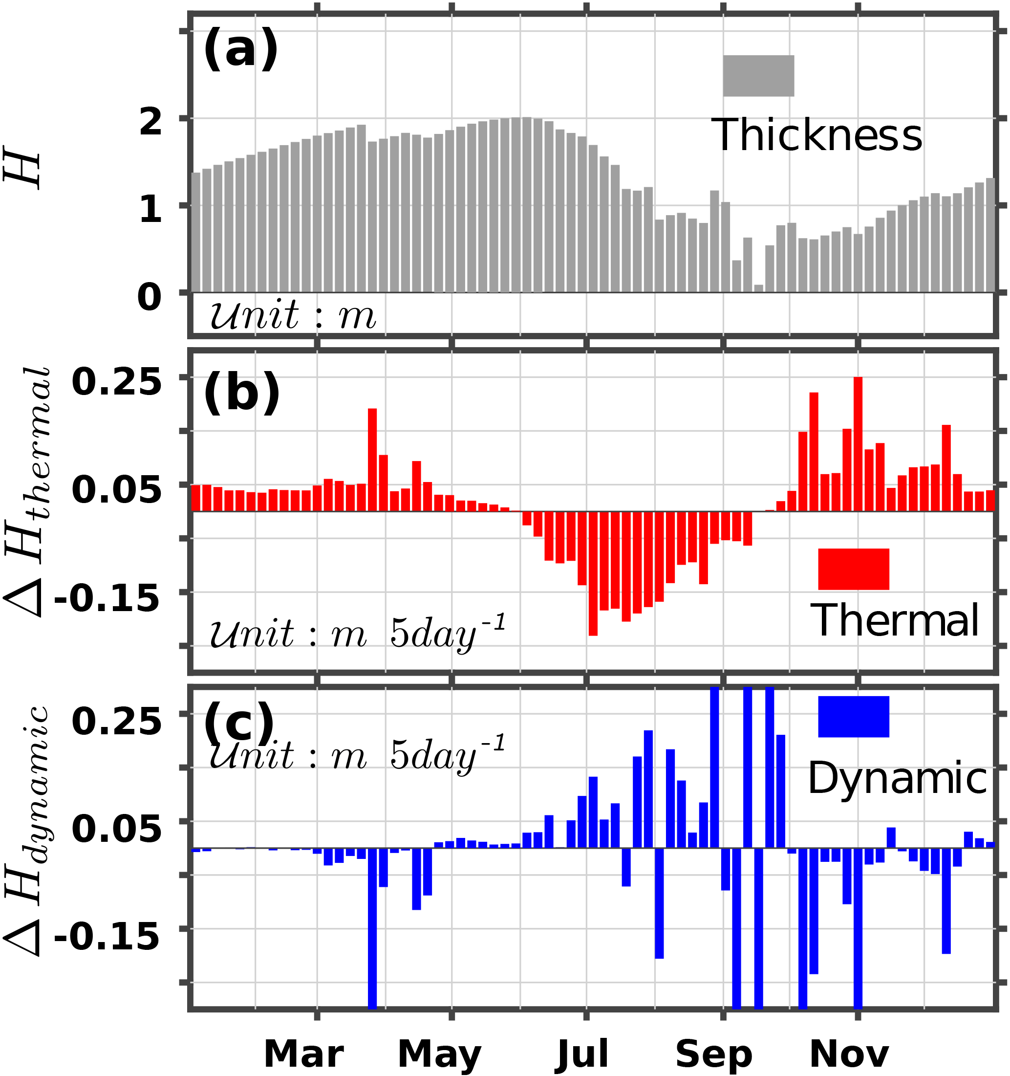
Figure 5Seasonal cycle (averaged over 2003 to 2016) of ice thickness (a, unit: metres), dynamic (b), and thermodynamic (c) ice thickness changes (unit: metres per 5-day) at Cambridge Bay from the ANHA12-CGRF simulation. Note each x grid line indicates the beginning of each month.
Figure 5 shows the seasonal cycle of ice thickness, 5-day ΔHdynamic and ΔHthermal averaged between 2003 and 2016 at Cambridge Bay. Sea ice reaches its maximal thickness (∼ 2 m) in late May with ice-free conditions for about 2 months (August and September). As the sea ice starts to form (October and November), both thermodynamics (e.g., due to cold temperature) and dynamics (e.g., local advection) play a role in the production of the ice thickness although with opposite contributions (Fig. 5b and c). Starting from December through to the end of the next May, it is almost a pure thermodynamic process that controls the ice thickness change. Note that the thermodynamic ice production is not constant in time; it is about 3 times larger in the first period (∼ 0.03 m per day) than in the later period (∼ 0.01 m per day). The steady thermodynamic growth in the second period contributes to about half of the total ice thickness. During the ice melting period (June and July), the thermodynamics is the major player as well (Fig. 5c).
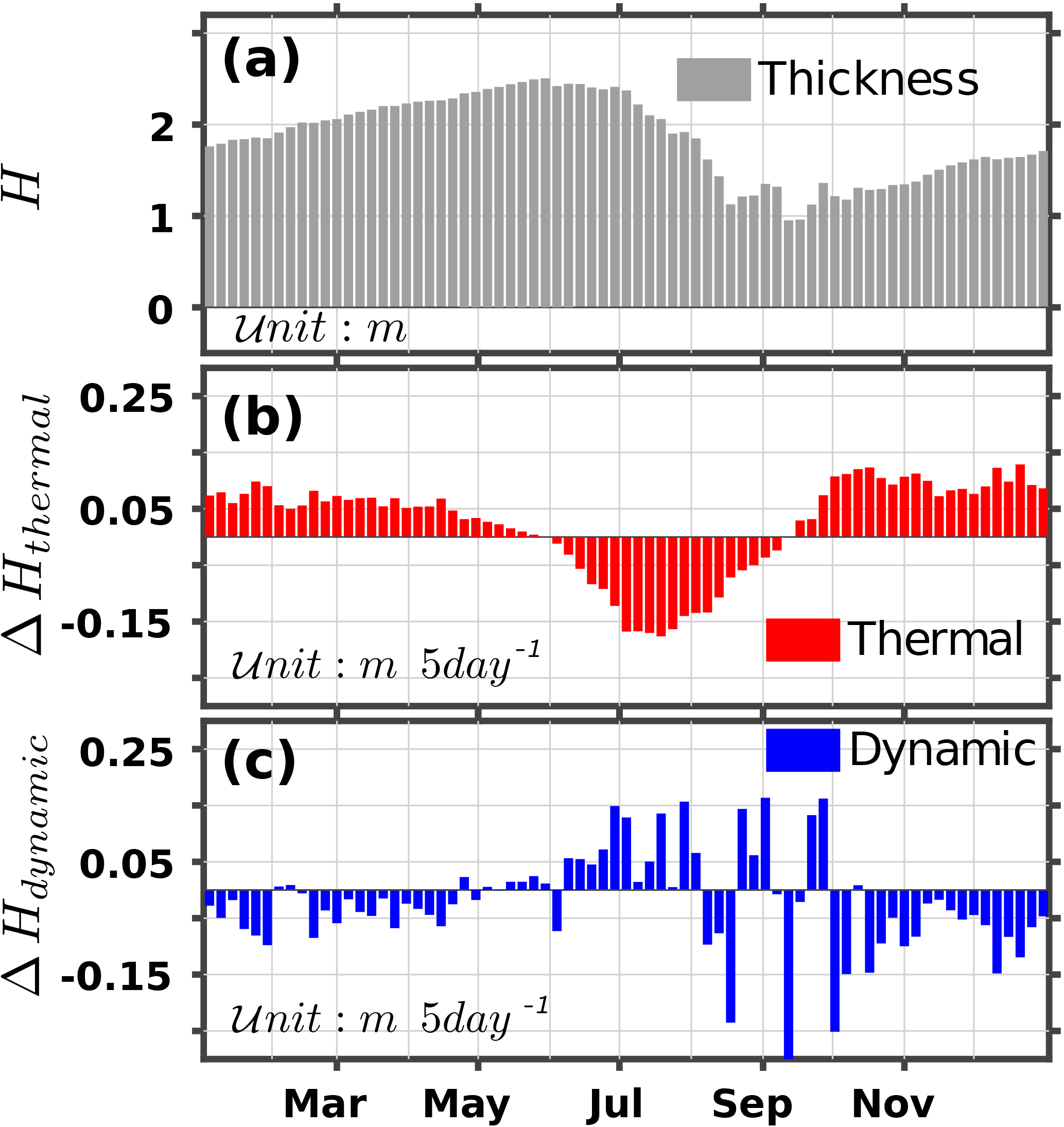
At Resolute, on average, there is no ice-free period (∼ 2.5 m at the end of May and ∼ 1 m in August and September) (Fig. 6a), although there is large interannual variability (Fig. 2a). For example, in 2012 there is an ice-free period in the middle of September (Fig. 7a). The freeze-up date is about half a month earlier at Resolute than that at Cambridge Bay. The ice production is a little larger at the beginning (October to December), ∼ 0.02 m per day, than later (Fig. 6b), ∼ 0.01 m per day, but the difference is not as noticeable as at Cambridge Bay (Fig. 5b). The relatively faster thermal growth lasts longer at Resolute than that at Cambridge Bay, likely due to local advection. These features are also applicable to a specific year, e.g., 2012 (Fig. 7). The non-thermodynamic contribution is more significant than at Resolute (Fig. 5c) but basically plays a negative role, i.e., slowing ice thickness increase during the winter season. Similarly to Cambridge Bay, the thermodynamics is the dominant factor melting the sea ice, with a melting peak in July. During the melting season, more ice can be advected to Resolute and melts later locally (Fig. 6c) than that at Cambridge (Fig. 5c).
3.3 Ice volume budget
3.3.1 Northern CAA
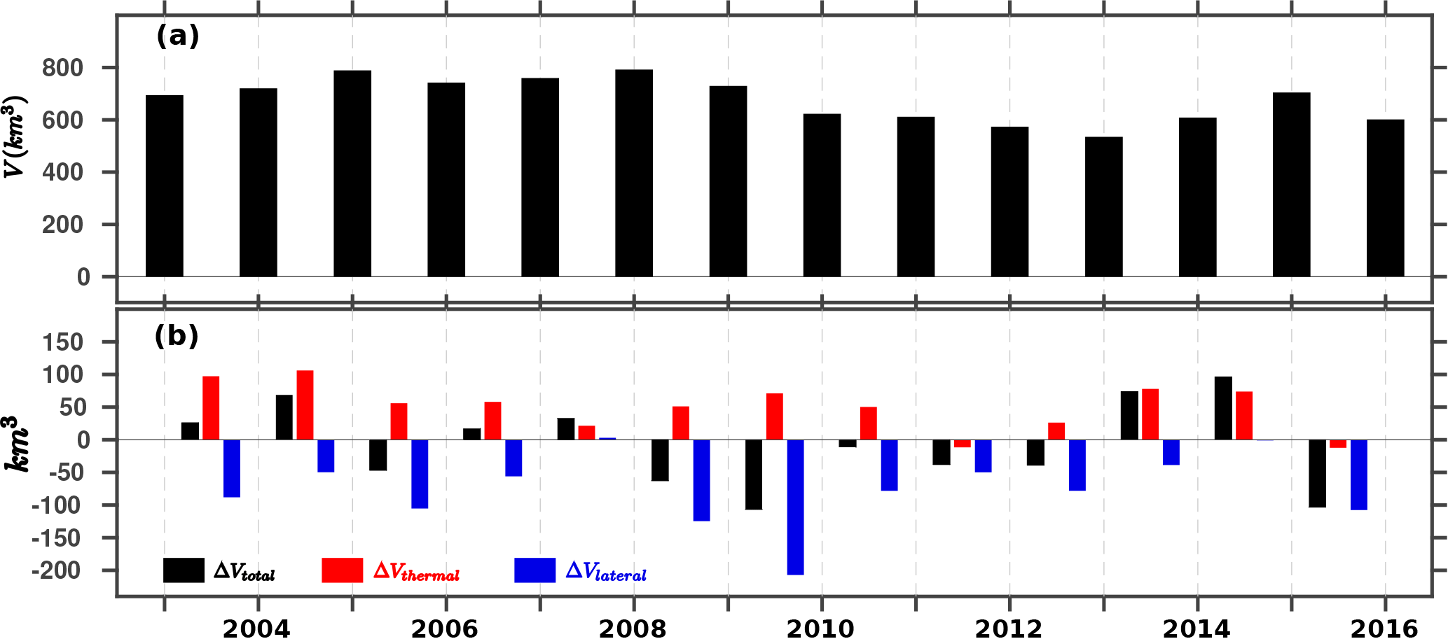
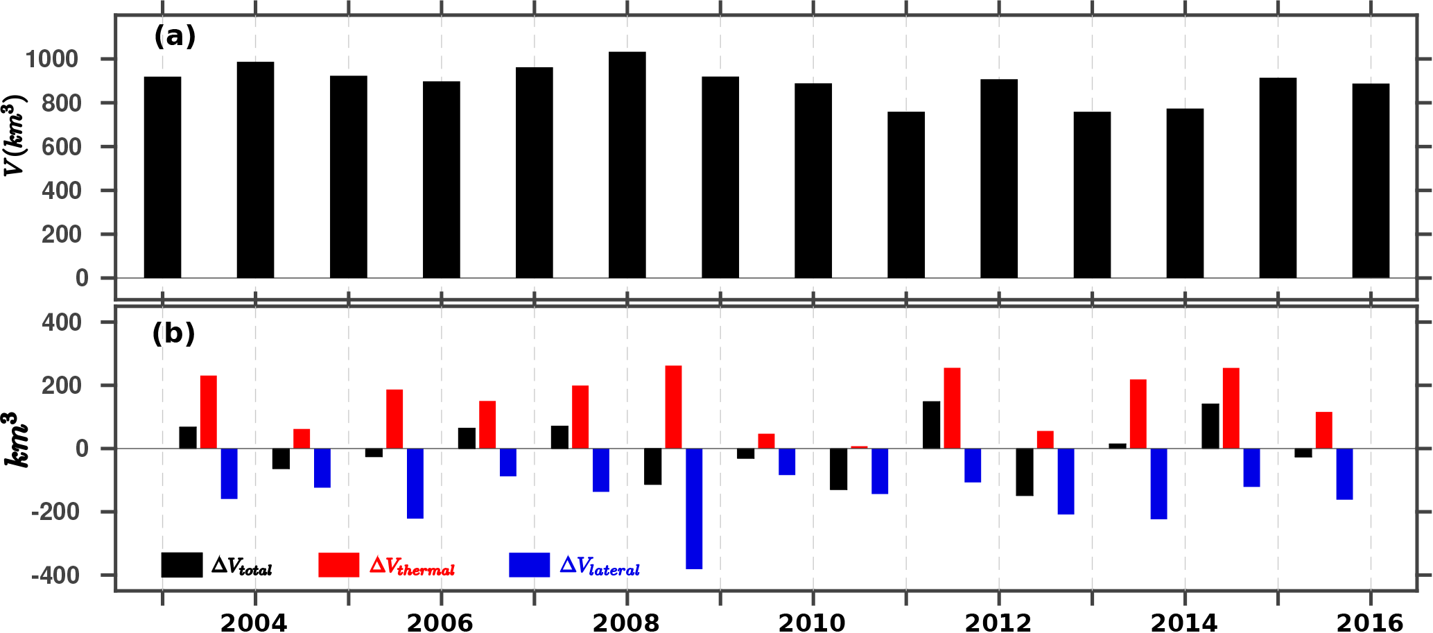
Figure 8Sea ice volume balance in the northern CAA (location see Fig. 1). (a) Maximum total ice volume (black bars, unit: km3) in each seasonal cycle (17 September to next 12 September). (b) The net ice volume change (black bars) between 2 consecutive years, thermodynamic ice volume change (red bars) and lateral ice volume transport (blue bars) in cubic kilometres.
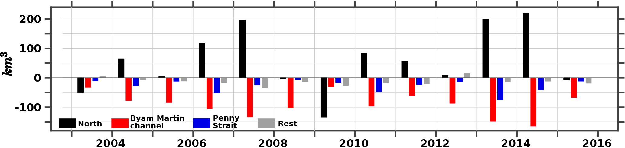
Figure 8a shows the maximum total ice volume (referred as “ice volume” hereafter if not mentioned specifically) in the northern CAA (solid black polygon shown in Fig. 1), which is covered by thick ice most of the year. An increase of 14 % (from 695 to 789 km3) in the ice volume is shown in the first 3 years. This is similar to the equilibrium problem we see at Eureka (Fig. 2g). During this period, the thermodynamic growth is the main contributor (203 km3) while the net lateral ice volume transport (−138 km3 per year) is out of this region (Fig. 8b), particular through Byam Martin Channel (Fig. 9). The sign convention is defined as positive means transport into the northern CAA regions. The ice volume stabilizes at high values for 4 years until 2008. After that, a shrinkage of about one-third (792 to 535 km3) in ice volume is simulated over 2008–2013. This reduction is due to large net lateral transport (Fig. 8b), e.g., in 2008 (−125 km3), 2009 (−207 km3), and 2012 (−78 km3). The large lateral transport is not always due to large outflow to the south, e.g., −102 km3 in 2008 and −96 km3 in 2010 through Byam Martin Channel and −48 km3 in 2010 through Penny Strait, but also could be caused by less import (e.g., 8 km3 in 2012) or even export (−134 km3 in 2009) through the northern gates (Fig. 9). It also shows that large import of ice through the northern gates is usually accompanied by large export to the south, mainly via Byam Martin Channel but also through Penny Strait in some years, e.g., 2010, 2013, and 2014. Both the thermodynamic and lateral transport (contribution through each major gate as well) experience significant interannual variations.
3.3.2 Parry Channel
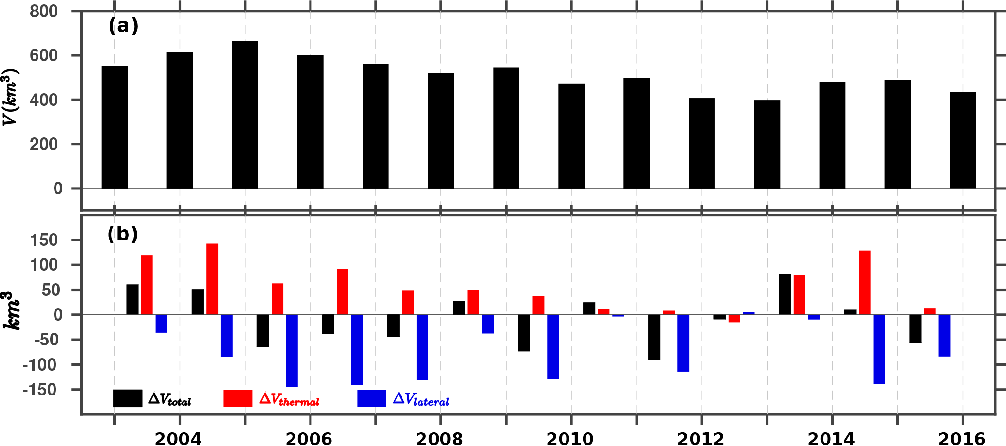
Parry Channel (dashed black polygon shown in Fig. 1) is the main water channel that connects the Arctic Ocean and Baffin Bay through the CAA (Fig. 1). It starts from M'Clure Strait on the west, running to east by the mouth of Lancaster Sound before entering Baffin Bay. Over the whole simulation, a decrease of 15.2 km3 per year (r2 = 0.66, p=0.0004) in the maximum ice volume is present (Fig. 10a). Even ignoring the initial increase over the first 3 years (from 554 km3 in 2003 to 665 km3 in 2005), the downward trend is similar (14.6 km3 per year with r2 = 0.58, p=0.0065). However, this decline is not steady but with interannual variability. The minima are found in 2012 (407 km3) and 2013 (398 km3), which are more than 20 % lower than the average, 524 km3. Similar to the northern CAA, thermodynamic growth is the main contributor to the ice volume increase from year to year while net lateral transport functions to deplete the sea ice (Fig. 10b).
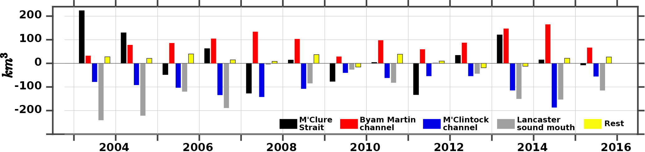
Large inflows from M'Clure Strait are simulated in the first 2 years (Fig. 11), but the direction of sea ice flow can switch from year to year (e.g., −132 km3 in 2011 and 120 km3 in 2013). The outflow events in 2007 and 2011 are consistent with the ice area flux study in Howell et al. (2013). As significant interannual variability in the amount of this ice volume flux is also present, the overall contribution of ice volume into Parry Channel from M'Clure Strait is small, which also supports the finding in Howell et al. (2013).
Major sea ice volume exchanges (Fig. 11) occur at Byam Martin Channel (inflow from the north), M'Clintock Channel (outflow to the south), and Lancaster Sound mouth (outflow to Baffin Bay). On average, annual ice volume fluxes through the first two routes nearly cancel each other (92 km3 vs. 94 km3), which indicates a relatively volume conservation due to high concentrations. The averaged sea ice transport at the east end (via Lancaster Sound mouth) is an export into Baffin Bay (92 km3 per year), which is closed to an early estimation (102 km3 per year) from Agnew et al. (2008).
3.3.3 Baffin Bay
Baffin Bay (dotted black polygon shown in Fig. 1), bounded by Smith Sound in the north, Jones Sound and Lancaster Sound in the west, and Davis Strait in the south (∼ 672× 103 km2), is covered by seasonal sea ice with an averaged maximum ice volume of 895 km3. No obvious decline is found over the simulation period (Fig. 12a). Although both the local thermodynamic ice growth and lateral ice volume flux show remarkable interannual variability (Fig. 12b), the balance between the contributions results in a relatively stable ice volume within the Bay.
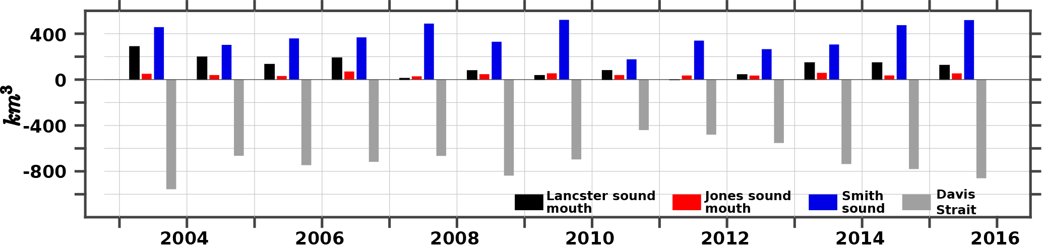
Figure 13 shows the lateral ice volume flux is dominated by the inflow from the northern (Smith Sound) and outflow from the south (Davis Strait). On the west side (via Lancaster Sound and Jones Sound), the direction of ice flux is mainly into Baffin Bay, but the total amount is much smaller than ice volume flux via either Smith Sound or Davis Strait. This is consistent with other studies (Agnew et al., 2008; Sou and Flato, 2009; Tang et al., 2004). The averaged export of ice volume flux through Davis Strait is 702 km3 per year with a standard deviation of 147 km3 per year. This number is larger than estimates in Curry et al. (2011, 2014): 500 and 424 km3, respectively. But they are not very different, taking account of the uncertainties in observations, large interannual variability, and difference in integration period (Baffin Bay ice volume maximals are used to determine the integration period in this study). It is more comparable to the 530–800 km3 per year estimated by Kwok (2007). In addition, the low outflow event in 2004 and high outflow event in 2008 agree with Curry et al. (2014). The inflow of ice flux from Smith Sound is 377 km3 per year, which is much larger than the long-term mean (9 km3 per year) in a coarse simulation done by Sou and Flato (2009), but closer to their estimate through southern Smith Sound section, i.e., 170 km3. It indicates sea ice in this region is more dynamic in our simulation (Fig. 4). This dynamic feature is also evidenced in ice motion vector fields derived from enhanced resolution Advanced Microwave Scanning Radiometer (AMSR-E) imagery in Agnew et al. (2008). Relatively large ice fluxes (e.g., 110 km3 per year in 1977–1978 and 136 km3 in 1974–1975) through Smith Sound were also estimated based on satellite images and a mean ice thickness of 2.5 m by Dey (1981). Another way to estimate the ice flux through Smith Sound is based on the ice flux through the north end of Nares Strait (i.e., Robeson Channel). Note ice flux through Smith Sound usually is larger than the sea ice influx through Nares Strait (Dey, 1981). Kwok et al. (2010) estimated the annual mean ice volume flux to 141 km3 per year over 2003–2008. The large outflow (254 km3) event in 2007 through Nares Strait reported by Kwok et al. (2010) is also seen in our simulation (Fig. 13). Both Sou and Flato (2009) and Terwisscha van Scheltinga et al. (2010) attributed the much-lower-than-observation ice flux through Nares Strait to wind forcing, which does not have enough resolution to resolve the along-strait winds. With a high-resolution wind forcing, Rasmussen et al. (2010) were able to reproduce much more reasonable ice flux through this narrow channel.
Increasing model horizontal resolution does not result in much noticeable change or improvement in sea ice thickness simulation, at least between 1∕4 and . We presented the sea ice thickness simulated within the CAA with a relatively simple (not multi-category) sea ice model, LIM2, with both 1∕4 and resolutions from 2002 to 2016. Simulations can capture the ice thickness asymmetric seasonal cycle and amplitude and compare reasonably well with the ECCC observations at most sites. In general, the difference is not visible between the runs with different horizontal resolutions. We expect model resolution to play a big role when it resolves much smaller scale, e.g., sufficient to resolve a ridge/lead. ANHA12 does show differences at Eureka (Fig. 2g), but this is related not to the sea ice model physics but rather to improvements in the local coastline, and thus to the regional circulation and the dynamic component (not shown). In regards to the model's horizontal resolution, our simulations do not have enough resolution to resolve the fjord process, which is important to study the hidden polynyas in Melling et al. (2015). This study focuses on the large-scale features; e.g., the simulations can produce reasonable spatial distribution of the thickness (very thick ice in the northern CAA, thick ice in the west-central Parry Channel, and thin ice in the eastern and southern regions of CAA).
The dynamic contribution should be considered in the offshore ice growth and basin-scale ice volume budget in the CAA. We studied the spatial distribution of the thermodynamic and dynamic ice growth in winter months. Relatively smaller thermodynamic contribution in the winter season is found in the thick ice-covered areas, with larger contributions in the thin ice-covered regions. Large dynamic ice growth is found along the northern CAA coast, the west of Bank Island, Byam Martin Channel, and northwest Baffin Bay region (e.g., Smith Sound, Jones Sound, and Lancaster Sound). On the basin scale, the interannual variations of the winter maximum ice volume in the northern CAA, Parry Channel and Baffin Bay are controlled by the thermodynamic growth and lateral transport. While both components demonstrate significant interannual variabilities, there is no clear trend in the winter maximum ice volume within the northern CAA and Baffin Bay regions but there is a downward trend (r2 ≈ 0.6) in Parry Channel region. In the northern CAA, the lateral transport is mainly through the northern gates and Byam Martin Channel but large ice volume flux could also flow south via Penny Strait when there is large inflow through the northern gates. Ice flow via Byam Martin Channel into Parry Channel is balanced by outflow into M'Clintock Channel on average. Eastward sea ice export through Lancaster Sound mouth is a big term in Parry Channel ice volume budget, but it is much smaller than the influx from Smith Sound and outflux through Davis Strait in the ice volume budget of Baffin Bay. These estimates are comparable to limited available studies, but further evaluations are still in need to confirm the quantities and variations.
It should be noted that landfast ice parameterizations and tides were not included in our simulations. The sea ice model utilized here does produce zero-motion sea ice (e.g., Fig. 4d), but more realistic physical parameterizations (Lemieux et al., 2016) are not applied in our simulations yet. With such parameterizations, we expect great improvements in simulating the widely existing landfast ice in the CAA region (Galley et al., 2012; Haas and Howell, 2015; Howell et al., 2016; Melling, 2002). Below the ice, tidal current plays an important role in the formation of open and hidden polynyas by enhancing mixing, bringing warm subsurface water towards surface or into fjords over the sills (Melling et al., 2015). Luneva et al. (2015) also showed there is much larger tidal impact on ice thickness in the CAA than the Arctic Ocean in numerical sensitivity experiments. Unfortunately, tides are not included in the ocean component of our current simulations. Thus, polynyas, the important features in this region, were not well produced in the simulations. We cannot study the detailed realistic physical formation processes proposed by Melling et al. (2015).
For access to the model data contact Paul G. Myers (pmyers@ualberta.ca).
The authors declare that they have no conflict of interest.
We
gratefully acknowledge the financial and logistic support of grants from the
Natural Sciences and Engineering Research Council (NSERC) of Canada. These
include a Discovery Grant (rgpin 227438-09) awarded to Paul G. Myers, Climate
Change and Atmospheric Research grants (VITALS, RGPCC 433898, and the
Canadian Arctic Geotraces program, RGPCC 433848), and Polar Knowledge
(432295). We are grateful to the NEMO development team and the Drakkar
project for providing the model and continuous guidance and to Westgrid and
Compute Canada for computational resources. We also thank Gregory
Smith for the CGRF forcing fields
that made available by Environment and Climate Change Canada. We appreciate
the Environment and Climate Change Canada New Arctic Ice Thickness Program
for providing valuable sea ice thickness measurements used in this study.
Greenland freshwater flux data analyzed in this study are presented in
Bamber et al. (2012) and are available on request as a gridded
product. We thank NCAR/UCAR for making Dai and Trenberth Global River Flow
and Continental Discharge Dataset available. We acknowledge WCRP/CLIVAR Ocean
Model Development Panel (OMDP) for sponsoring and organizing the Coordinated
Ocean-sea ice Reference Experiments (CORE) dataset. We also acknowledge
Mercator Ocean for providing the GLORYS model output for initial and open
boundary conditions. The GLORYS reanalysis project is carried out in the
framework of the European Copernicus Marine Environment Monitoring Service
(CMEMS). We also appreciate the three anonymous reviewers for their valuable
comments, which have greatly improved this
paper.
Edited by: Christian Haas
Reviewed by: three anonymous referees
Agnew, T., Lambe, A., and Long, D.: Estimating sea ice area flux across the Canadian Arctic Archipelago using enhanced AMSR-E, J. Geophys. Res., 113, C10011, https://doi.org/10.1029/2007JC004582, 2008. a, b, c, d
Bailey, W. B.: Oceanographic Features of the Canadian Archipelago, J. Fish. Res. Board Can., 14, 731–769, https://doi.org/10.1139/f57-030, 1957. a
Bamber, J., van den Broeke, M., Ettema, J., Lenaerts, J., and Rignot, E.: Recent large increases in freshwater fluxes from Greenland into the North Atlantic, Geophys. Res. Lett., 39, L19501, https://doi.org/10.1029/2012GL052552, 2012. a, b
Bouillon, S., Fichefet, T., Legat, V., and Madec, G.: The elastic–viscous–plastic method revisited, Ocean Model., 71, 2–12, 2013. a
Brown, R. D. and Cote, P.: Interannual variability of landfast ice thickness in the Canadian High Arctic, 1950–89, Arctic, 45, 273–284, 1992. a
CIS: Sea Ice Climatic Atlas: Northern Canadian Waters, 1981–2010, available at: http://publications.gc.ca/site/eng/441147/publication.html (last access: 11 December 2017), 2011. a
Comiso, J. C., Parkinson, C. L., Gersten, R., and Stock, L.: Accelerated decline in the Arctic sea ice cover, Geophys. Res. Lett., 35, L01703, https://doi.org/10.1029/2007GL031972, 2008. a
Curry, B., Lee, C. M., and Petrie, B.: Volume, freshwater, and heat fluxes through Davis Strait, 2004–05, J. Phys. Oceanogr., 41, 429–436, https://doi.org/10.1175/2010JPO4536.1, 2011. a
Curry, B., Lee, C. M., Petrie, B., Moritz, R. E., and Kwok, R.: Multiyear Volume, Liquid Freshwater, and Sea Ice Transports through Davis Strait, 2004-10*, J. Phys. Oceanogr., 44, 1244–1266, https://doi.org/10.1175/JPO-D-13-0177.1, 2014. a, b
Dai, A., Qian, T., Trenberth, K. E., and Milliman, J. D.: Changes in continental freshwater discharge from 1948 to 2004, J. Climate, 22, 2773–2792, 2009. a
Dey, B.: Monitoring winter sea ice dynamics in the Canadian Arctic with NOAA-TIR images, J. Geophys. Res., 86, 3223–3235, https://doi.org/10.1029/JC086iC04p03223, 1981. a, b
Dickson, R., Rudels, B., Dye, S., Karcher, M., Meincke, J., and Yashayaev, I.: Current estimates of freshwater flux through Arctic and subarctic seas, Prog. Oceanogr., 73, 210–230, 2007. a
Drakkar Group: Eddy-permitting ocean circulation hindcasts of past decades, CLIVAR Exchanges, 42, 8–10, 2007. a
Dumas, J. A., Flato, G. M., and Brown, R. D.: Future projections of landfast ice thickness and duration in the Canadian Arctic, J. Climate, 19, 5175–5189, 2006. a, b, c, d
Dunbar, M.: The geographical position of the North Water, Arctic, 22, 438–441, 1969. a
Fichefet, T. and Maqueda, M. A. M.: Sensitivity of a global sea ice model to the treatment of ice thermodynamics and dynamics, J. Geophys. Res., 102, 12609–12646, https://doi.org/10.1029/97JC00480, 1997. a
Flato, G. M. and Brown, R. D.: Variability and climate sensitivity of landfast Arctic sea ice, J. Geophys. Res., 101, 25767–25777, https://doi.org/10.1029/96JC02431, 1996. a
Galley, R. J., Else, B. G., Howell, S. E., Lukovich, J. V., and Barber, D. G.: Landfast sea ice conditions in the Canadian Arctic: 1983–2009, Arctic, 65, 133–144, 2012. a
Haas, C. and Howell, S. E. L.: Ice thickness in the Northwest Passage, Geophys. Res. Lett., 42, 7673–7680, https://doi.org/10.1002/2015GL065704, 2015. a, b, c, d, e, f
Hátún, H., Sandø, A. B., Drange, H., Hansen, B., and Valdimarsson, H.: Influence of the Atlantic subpolar gyre on the thermohaline circulation, Science, 309, 1841–1844, 2005. a
Howell, S. E. L., Tivy, A., Yackel, J. J., and McCourt, S.: Multi-year sea-ice conditions in the western Canadian Arctic Archipelago region of the Northwest Passage: 1968-2006, Atmos. Ocean, 46, 229–242, 2008. a, b, c, d
Howell, S. E. L., Duguay, C. R., and Markus, T.: Sea ice conditions and melt season duration variability within the Canadian Arctic Archipelago: 1979–2008, Geophys. Res. Lett., 36, L10502, https://doi.org/10.1029/2009GL037681, 2009. a, b, c
Howell, S. E. L., Wohlleben, T., Dabboor, M., Derksen, C., Komarov, A., and Pizzolato, L.: Recent changes in the exchange of sea ice between the Arctic Ocean and the Canadian Arctic Archipelago, J. Geophys. Res.-Oceans, 118, 3595–3607, https://doi.org/10.1002/jgrc.20265, 2013. a, b, c, d
Howell, S. E. L., Laliberté, F., Kwok, R., Derksen, C., and King, J.: Landfast ice thickness in the Canadian Arctic Archipelago from observations and models, The Cryosphere, 10, 1463–1475, https://doi.org/10.5194/tc-10-1463-2016, 2016. a, b, c, d, e, f
Hu, X. and Myers, P. G.: Changes to the Canadian Arctic Archipelago Sea Ice and Freshwater Fluxes in the Twenty-First Century under the Intergovernmental Panel on Climate Change A1B Climate Scenario, Atmos. Ocean, 52, 331–350, https://doi.org/10.1080/07055900.2014.942592, 2014. a
Hunke, E. C. and Dukowicz, J. K.: An elastic-viscous-plastic model for sea ice dynamics, J. Phys. Oceanogr., 27, 1849–1867, 1997. a, b
Kwok, R.: Exchange of sea ice between the Arctic Ocean and the Canadian Arctic Archipelago, Geophys. Res. Lett., 33, L16501, https://doi.org/10.1029/2006GL027094, 2006. a
Kwok, R.: Baffin Bay ice drift and export: 2002–2007, Geophys. Res. Lett., 34, L19501, https://doi.org/10.1029/2007GL031204, 2007. a
Kwok, R.: Sea ice convergence along the Arctic coasts of Greenland and the Canadian Arctic Archipelago: Variability and extremes (1992–2014), Geophys. Res. Lett., 42, 7598–7605, 2015. a
Kwok, R. and Cunningham, G. F.: Variability of Arctic sea ice thickness and volume from CryoSat-2, Philos. T. R. Soc. A, 373, 20140157, https://doi.org/10.1098/rsta.2014.0157, 2015. a
Kwok, R., Toudal Pedersen, L., Gudmandsen, P., and Pang, S. S.: Large sea ice outflow into the Nares Strait in 2007, Geophys. Res. Lett., 37, L03502, https://doi.org/10.1029/2009GL041872, 2010. a, b
Large, W. G. and Yeager, S. G.: The global climatology of an interannually varying air–sea flux data set, Clim. Dynam., 33, 341–364, 2009. a
Laxon, S. W., Giles, K. A., Ridout, A. L., Wingham, D. J., Willatt, R., Cullen, R., Kwok, R., Schweiger, A., Zhang, J., Haas, C., Stefan Hendricks, S., Krishfield, R., Kurtz, N., Farrell, S., and Davidson, M.: CryoSat-2 estimates of Arctic sea ice thickness and volume, Geophys. Res. Lett., 40, 732–737, 2013. a
Lemieux, J.-F., Knoll, D. A., Tremblay, B., Holland, D. M., and Losch, M.: A comparison of the Jacobian-free Newton–Krylov method and the EVP model for solving the sea ice momentum equation with a viscous-plastic formulation: a serial algorithm study, J. Comput. Phys., 231, 5926–5944, 2012. a
Lemieux, J.-F., Dupont, F., Blain, P., Roy, F., Smith, G. C., and Flato, G. M.: Improving the simulation of landfast ice by combining tensile strength and a parameterization for grounded ridges, J. Geophys Res.-Oceans, 121, 7354–7368, 2016. a, b
Lietaer, O., Fichefet, T., and Legat, V.: The effects of resolving the Canadian Arctic Archipelago in a finite element sea ice model, Ocean Model., 24, 140–152, 2008. a
Luneva, M. V., Aksenov, Y., Harle, J. D., and Holt, J. T.: The effects of tides on the water mass mixing and sea ice in the Arctic Ocean, J. Geophys. Res.-Oceans, 120, 6669–6699, 2015. a
Madec, G. and the NEMO team: NEMO ocean engine, Note du Pôle de modélisation, Institut Pierre-Simon Laplace (IPSL), France, No 27, ISSN No 1288-1619, 2008. a
Marshall, J., Kushnir, Y., Battisti, D., Chang, P., Czaja, A., Dickson, R., Hurrell, J., McCartney, M., Saravanan, R., and Visbeck, M.: North Atlantic climate variability: phenomena, impacts and mechanisms, Int. J. Climatol., 21, 1863–1898, 2001. a
Masina, S., Storto, A., Ferry, N., Valdivieso, M., Haines, K., Balmaseda, M., Zuo, H., Drevillon, M., and Parent, P.: Clim. Dynam., 49, 813, https://doi.org/10.1007/s00382-015-2728-5, 2017. a
Maslanik, J., Stroeve, J., Fowler, C., and Emery, W.: Distribution and trends in Arctic sea ice age through spring 2011, Geophys. Res. Lett., 38, https://doi.org/10.1029/2011GL047735, 2011. a
Melling, H.: Sea ice of the northern Canadian Arctic Archipelago, J. Geophys. Res., 107, 3181, https://doi.org/10.1029/2001JC001102, 2002. a, b, c, d, e, f
Melling, H., Gratton, Y., and Ingram, G.: Ocean circulation within the North Water polynya of Baffin Bay, Atmos. Ocean, 39, 301–325, https://doi.org/10.1080/07055900.2001.9649683, 2001. a
Melling, H., Agnew, T., Falkner, K. K., Greenberg, D. A., Lee, C. M., Münchow, A., Petrie, B., Prinsenberg, S. J., Samelson, R. M., and Woodgate, R. A.: Fresh-water fluxes via Pacific and Arctic outflows across the Canadian polar shelf, Arctic-Subarctic Ocean Fluxes: Defining the Role of the Northern Seas in Climate, 193–247, 2008. a
Melling, H., Haas, C., and Brossier, E.: Invisible polynyas: Modulation of fast ice thickness by ocean heat flux on the Canadian polar shelf, J. Geophys. Res.-Oceans, 120, 777–795, https://doi.org/10.1002/2014JC010404, 2015. a, b, c
Mudryk, L., Derksen, C., Howell, S., Laliberté, F., Thackeray, C., Sospedra-Alfonso, R., Vionnet, V., Kushner, P., and Brown, R.: Canadian Snow and Sea Ice: Trends (1981–2015) and Projections (2020–2050), The Cryosphere Discuss., https://doi.org/10.5194/tc-2017-198, in review, 2017. a
Parkinson, C. L. and Cavalieri, D. J.: Arctic sea ice variability and trends, 1979–2006, J. Geophys. Res., 113, C07003, https://doi.org/10.1029/2007JC004558, 2008. a
Parkinson, C. L. and Comiso, J. C.: On the 2012 record low Arctic sea ice cover: Combined impact of preconditioning and an August storm, Geophys. Res. Lett., 40, 1356–1361, https://doi.org/10.1002/grl.50349, 2013. a
Parkinson, C. L., Cavalieri, D. J., Gloersen, P., Zwally, H. J., and Comiso, J. C.: Arctic sea ice extents, areas, and trends, 1978–1996, J. Geophys. Res., 104, 20837–20856, 1999. a
Peterson, I., Hamilton, J., Prinsenberg, S., and Pettipas, R.: Wind-forcing of volume transport through Lancaster Sound, J. Geophys. Res., 117, C11018, https://doi.org/10.1029/2012JC008140, 2012. a
Pizzolato, L., Howell, S. E. L., Derksen, C., Dawson, J., and Copland, L.: Changing sea ice conditions and marine transportation activity in Canadian Arctic waters between 1990 and 2012, Climatic Change, 123, 161–173, https://doi.org/10.1007/s10584-013-1038-3, 2014. a
Pizzolato, L., Howell, S. E. L., Dawson, J., Laliberté, F., and Copland, L.: The influence of declining sea ice on shipping activity in the Canadian Arctic, Geophys. Res. Lett., 43, 12146–12154, https://doi.org/10.1002/2016GL071489, 2016. a
Prinsenberg, S. J. and Hamilton, J.: Monitoring the volume, freshwater and heat fluxes passing through Lancaster Sound in the Canadian Arctic Archipelago, Atmos. Ocean, 43, 1–22, https://doi.org/10.3137/ao.430101, 2005. a
Rasmussen, T. A. S., Kliem, N., and Kaas, E.: Modelling the sea ice in the Nares Strait, Ocean Model., 35, 161–172, https://doi.org/10.1016/j.ocemod.2010.07.003, 2010. a
Renka, R. J.: Multivariate interpolation of large sets of scattered data, ACM T. Math. Software, 14, 139–148, https://doi.org/10.1145/45054.45055, 1988. a
Rhein, M., Kieke, D., Hüttl-Kabus, S., Roessler, A., Mertens, C., Meissner, R., Klein, B., Böning, C. W., and Yashayaev, I.: Deep water formation, the subpolar gyre, and the meridional overturning circulation in the subpolar North Atlantic, Deep-Sea Res. Pt. II, 58, 1819–1832, 2011. a
Semtner Jr., A. J.: A model for the thermodynamic growth of sea ice in numerical investigations of climate, J. Phys. Oceanogr., 6, 379–389, 1976. a
Serreze, M. C., Holland, M. M., and Stroeve, J.: Perspectives on the Arctic's shrinking sea-ice cover, Science, 315, 1533–1536, 2007. a
Smith, G. C., Roy, F., Mann, P., Dupont, F., Brasnett, B., Lemieux, J.-F., Laroche, S., and Bélair, S.: A new atmospheric dataset for forcing ice–ocean models: Evaluation of reforecasts using the Canadian global deterministic prediction system, Q. J. Roy. Meteor. Soc., 140, 881–894, 2014. a
Sou, T. and Flato, G.: Sea ice in the Canadian Arctic Archipelago: Modeling the past (1950–2004) and the future (2041–60), J. Climate, 22, 2181–2198, 2009. a, b, c, d
Stroeve, J., Serreze, M., Drobot, S., Gearheard, S., Holland, M., Maslanik, J., Meier, W., and Scambos, T.: Arctic sea ice extent plummets in 2007, Eos, Transactions American Geophysical Union, 89, 13–14, 2008. a
Tang, C. C. L., Ross, C. K., Yao, T., Petrie, B., DeTracey, B. M., and Dunlap, E.: The circulation, water masses and sea-ice of Baffin Bay, Prog. Oceanogr., 63, 183–228, 2004. a
Terwisscha van Scheltinga, A. D., Myers, P. G., and Pietrzak, J. D.: A finite element sea ice model of the Canadian Arctic Archipelago, Ocean Dynam., 60, 1539–1558, https://doi.org/10.1007/s10236-010-0356-5, 2010. a
Tilling, R. L., Ridout, A., Shepherd, A., and Wingham, D. J.: Increased Arctic sea ice volume after anomalously low melting in 2013, Nat. Geosci., 8, 643–646, 2015. a
Tilling, R. L., Ridout, A., and Shepherd, A.: Estimating Arctic sea ice thickness and volume using CryoSat-2 radar altimeter data, Adv. Space Res., https://doi.org/10.1016/j.asr.2017.10.051, 2018. a
Vellinga, M. and Wood, R. A.: Global climatic impacts of a collapse of the Atlantic thermohaline circulation, Climatic Change, 54, 251–267, 2002. a
Williams, J., Tremblay, L. B., and Lemieux, J.-F.: The effects of plastic waves on the numerical convergence of the viscous–plastic and elastic–viscous–plastic sea-ice models, J. Comput. Phys., 340, 519–533, 2017. a