Canadian snow and sea ice: assessment of snow, sea ice, and related climate processes in Canada's Earth system model and climate-prediction system

The Canadian Sea Ice and Snow Evolution (CanSISE) Network is a climate research network focused on developing and applying state-of-the-art observational data to advance dynamical prediction, projections, and understanding of seasonal snow cover and sea ice in Canada and the circumpolar Arctic. This study presents an assessment from the CanSISE Network of the ability of the second-generation Canadian Earth System Model (CanESM2) and the Canadian Seasonal to Interannual Prediction System (CanSIPS) to simulate and predict snow and sea ice from seasonal to multi-decadal timescales, with a focus on the Canadian sector. To account for observational uncertainty, model structural uncertainty, and internal climate variability, the analysis uses multi-source observations, multiple Earth system models (ESMs) in Phase 5 of the Coupled Model Intercomparison Project (CMIP5), and large initial-condition ensembles of CanESM2 and other models. It is found that the ability of the CanESM2 simulation to capture snow-related climate parameters, such as cold-region surface temperature and precipitation, lies within the range of currently available international models. Accounting for the considerable disagreement among satellite-era observational datasets on the distribution of snow water equivalent, CanESM2 has too much springtime snow mass over Canada, reflecting a broader northern hemispheric positive bias. Biases in seasonal snow cover extent are generally less pronounced. CanESM2 also exhibits retreat of springtime snow generally greater than observational estimates, after accounting for observational uncertainty and internal variability. Sea ice is biased low in the Canadian Arctic, which makes it difficult to assess the realism of long-term sea ice trends there. The strengths and weaknesses of the modelling system need to be understood as a practical tradeoff: the Canadian models are relatively inexpensive computationally because of their moderate resolution, thus enabling their use in operational seasonal prediction and for generating large ensembles of multidecadal simulations. Improvements in climate-prediction systems like CanSIPS rely not just on simulation quality but also on using novel observational constraints and the ready transfer of research to an operational setting. Improvements in seasonal forecasting practice arising from recent research include accurate initialization of snow and frozen soil, accounting for observational uncertainty in forecast verification, and sea ice thickness initialization using statistical predictors available in real time.

1 Introduction

Seasonal snow cover and sea ice are integral to the cultural identity, history, and economy of northern nations like Canada. They also exert an enormous physical influence on the Earth system, ranging from local interactions with winds and temperatures in the Arctic and snow-covered regions, to larger-scale interactions with weather systems and ocean circulation, to global-scale influences on the Earth's energy balance. In recent decades, dramatic changes in Canada's snow cover and sea ice have been witnessed and documented (Derksen et al., 2012; Najafi et al., 2016). This has driven the need to better understand and predict these fields for the coming seasons, years, and decades. To address this need, Canada has helped lead the global effort to better observe and model snow, sea ice, and related climate parameters (such as northern high-latitude land-surface temperature and precipitation). This effort includes Canadian contributions to the International Polar Year (e.g. Kulkarni et al., 2012), to the development of Earth system model (ESM) and climate-prediction systems (Merryfield et al., 2013a; Sigmond et al., 2013; van den Hurk et al., 2016), and to leadership of ongoing field and remote sensing efforts (King et al., 2015).

As part of Canada's larger effort in snow and sea ice research, the focus here is on seasonal and longer timescale prediction of terrestrial snow, sea ice cover, and related climate variability. The purpose of this paper is to evaluate the ability of Canada's current ESM and climate-prediction system to carry out this kind of prediction in the context of the development of new observational products. This work was undertaken by the Canadian Sea Ice and Snow Evolution Network (CanSISE), a core project of the Climate Change and Atmospheric Research Program of the Natural Sciences and Engineering Research Council of Canada (CCAR/NSERC)¹. Model evaluation, which typically compares a model to observations, needs to account for several sources of uncertainty, including impacts of spatial and temporal sampling in the presence of internal climate variability and observational uncertainty (whether instrumental error or errors related to data processing and retrieval systems). Our evaluation of Canadian models is helped by ready access and comparison with output from internationally available models, to provide a suitable scientific context.

This study focuses on snow, sea ice, and related climate parameters and processes relevant to the Canadian land mass and the pan-Arctic region. The Canadian ESM and climate-prediction system has been studied in a variety of related settings (e.g. Arora et al., 2011; Merryfield et al., 2013a, b; Gillet et al., 2012; Sigmond et al., 2013; Kirtman et al., 2013; Flato et al., 2013). We here seek to more fully assess simulation and prediction of seasonal snow cover and regional sea ice variability accompanied by a more complete characterization of observational uncertainty, model structural uncertainty, and internal climate variability. After reviewing the current-generation Canadian Seasonal to Interannual Prediction System and the second-generation Canadian Earth System Model (CanSIPS and CanESM2, respectively; Sect. 2), we characterize climatological behaviour and trends for snow and sea ice in these systems (Sect. 3), provide an overview of recent developments in seasonal snow and sea ice prediction (Sect. 4), and conclude (Sect. 5) with a summary and discussion of new directions for prediction system development.

A companion paper from the CanSISE Network (Mudryk et al., 2018) assesses 1981–2015 trends and 2020–2050 projections of Canadian snow cover and sea ice.

2 Models and data used

In Sect. 3, our analysis will focus on CanESM2 (Arora et al., 2011; Scinocca et al., 2016). This is the ESM used by the Canadian Centre for Climate Modelling and Analysis (CCCma) of Environment and Climate Change Canada (ECCC) for its contribution to Phase 5 of the Coupled Model Intercomparison Project (CMIP5). CanESM2 combines atmosphere, ocean, land-surface (including snow), sea ice, and carbon-cycle components in a coupled framework in which all model components interact. The system can simulate the past and projected state of global temperature, circulation, carbon dioxide concentrations, etc. under the influence of external forcing, but independently of assimilated ocean and atmospheric initialization data. As summarized in Arora et al. (2011), the atmospheric and oceanic components are the fourth-generation atmospheric and oceanic general circulation models CanAM4 and CanOM4, the prognostic carbon-cycle components are the Canadian Model of Ocean Carbon (CMOC) and the Canadian Terrestrial Ecosystem Model (CTEM), the land-surface component (including the snow scheme) is version 3 of the Canadian Land Surface Scheme (CLASS), and the sea ice component is the Flato and Hibler (1992) cavitating fluid scheme. As with most other models participating in CMIP5, CanESM2 does not use flux adjustments that artificially constrain the climate system to be in a state of energy and water balance. Following CMIP5 protocols, the model includes concentrations and emissions of greenhouse gases, aerosol and aerosol-precursor emissions, and prescriptions for land-cover change (Arora et al., 2011).

CanESM2 has moderate spatial resolution compared to other CMIP5 models (approximately 2.8^∘ horizontal grid spacing and up to 35 vertical levels in the atmosphere; approximately 100 km horizontal grid spacing and up to 40 levels in the ocean). This resolution accounts for constraints on available computing resources. It sufficiently resolves salient features of the global atmospheric ocean circulation while still permitting the execution of large initial-condition ensembles of model simulations to adequately sample internal variability under different external forcings. We note that ECCC has also made a complementary multi-year investment in regional climate modelling (Scinocca et al., 2016) to provide higher resolution over North America (with versions at 50 and at 25 km grid resolution) to address the shortcomings of coarse resolution.

In Sect. 4, we consider the application over Canada of CanSIPS (Merryfield et al., 2013a), the operational prediction system of the Canadian Meteorological Centre (CMC) for climate variability on seasonal to interannual (several-month to multiple-year) timescales. Like CanESM2, CanSIPS is also a multi-component interactive system. However, unlike CanESM2, when operating as a prediction system CanSIPS starts from an initial state that approximates the real-world state at a given initial time. CanSIPS includes (1) a data assimilation system that estimates realistic initial states of the atmosphere, ocean, land, and sea ice to start the forecasts; (2) two separate coupled climate models (the earlier-generation Canadian Coupled Model 3, CanCM3; and the later-generation Canadian Coupled Model, CanCM4) that advance the simulated system from this initial condition (using an ensemble size of 10 for each model); and (3) diagnostic systems to analyze the output and generate useful forecasts for operational use within ECCC's Meteorological Service of Canada (e.g. Fig. 14 below and the probabilistic seasonal forecast at https://weather.gc.ca/saisons/prob_e.html). Evaluations of CanSIPS need to consider all three parts of the seasonal prediction system. CanCM4 has the same atmosphere, ocean, land, and sea ice components as CanESM2, but does not include CanESM2's carbon-cycle components. CanCM3 has the previous-generation atmosphere and ocean components relative to CanCM4 and CanESM2, but the same land-surface and sea ice components as CanCM4 and CanESM2 (Merryfield et al., 2013a).

Merryfield et al. (2013a) summarize the performance of CanCM3 and CanCM4 when the models are run independently of assimilated data. CanCM4 reduces the global mean absolute error of ocean surface temperatures compared to CanCM3, indicating an overall improvement in the coupled ocean–atmosphere state that results from improved physical parameterizations and finer resolution. Relative to CanCM3 and observations, CanCM4 tends to warm more rapidly under the effects of anthropogenic radiative forcing over the 1970–2009 period. In CanCM3, the simulation is characterized by excessive pan-Arctic sea ice cover in summer and winter and a small rate of sea ice loss compared to observations. In CanCM4, while there is still excessive sea ice cover in winter, there is too little sea ice in summer (see Sect. 3 below). The rate of sea ice loss in CanCM4 is more in line with recent observations than that in CanCM3 (Stroeve et al., 2012); however, caution is required to interpret recent sea ice loss rates in light of the large amount of multidecadal variability expected in these trends (e.g. Notz, 2012; Swart et al., 2015). Because CMIP5 simulations were carried out with CanESM2 but not CanCM4, the simulations required to do a clean comparison of CanCM4 and CanESM2, and thus gauge the impact of carbon-cycle processes on simulation quality, are not available.

When run as a prediction system, CanSIPS, combining CanCM3 and CanCM4, is able to show multi-month skill in seasonal forecasts of detrended sea ice area anomalies, comparable to that obtained in other modelling systems (Merryfield et al., 2013b), and generally enhanced skill relative to a statistical persistence forecast (Sigmond et al., 2013). The assessed skill depends on the verification dataset (Sigmond et al., 2013), especially for total (non-detrended) anomalies. Such issues will be revisited in this study.

Our assessment of CanSIPS and CanESM2 is enhanced by two recent research products arising from CanSISE: the Blended-5 snow water equivalent (SWE) dataset of Mudryk et al. (2015) and the CanESM2-LE (large ensemble) of simulations from CanESM2. The Blended-5 dataset addresses the need for a SWE verification dataset and, potentially, for initialization of snow-related parameters in CanSIPS and other prediction systems. Blended-5 builds on long-term work of ECCC (e.g. Brown et al., 2010; Derksen and Brown, 2012; Brown and Derksen, 2013) and consists of an ensemble of gridded SWE datasets over 1981–2010 from a variety of sources including remote sensing, land-surface assimilation systems, and reanalysis-driven snow models. The papers of Mudryk et al. (2015, 2017) detail the components, quality assessment, and characteristics of the Blended-5 dataset.

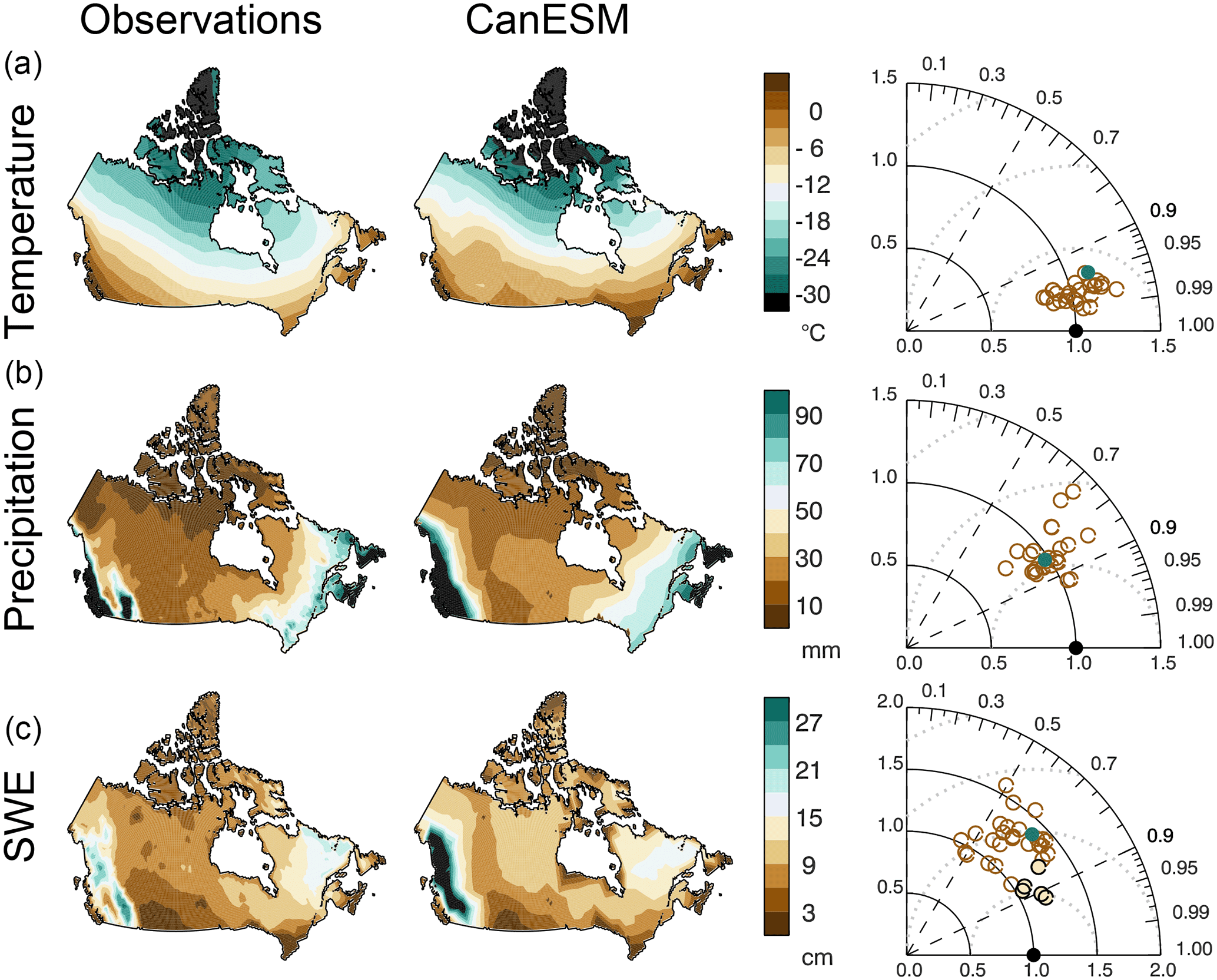
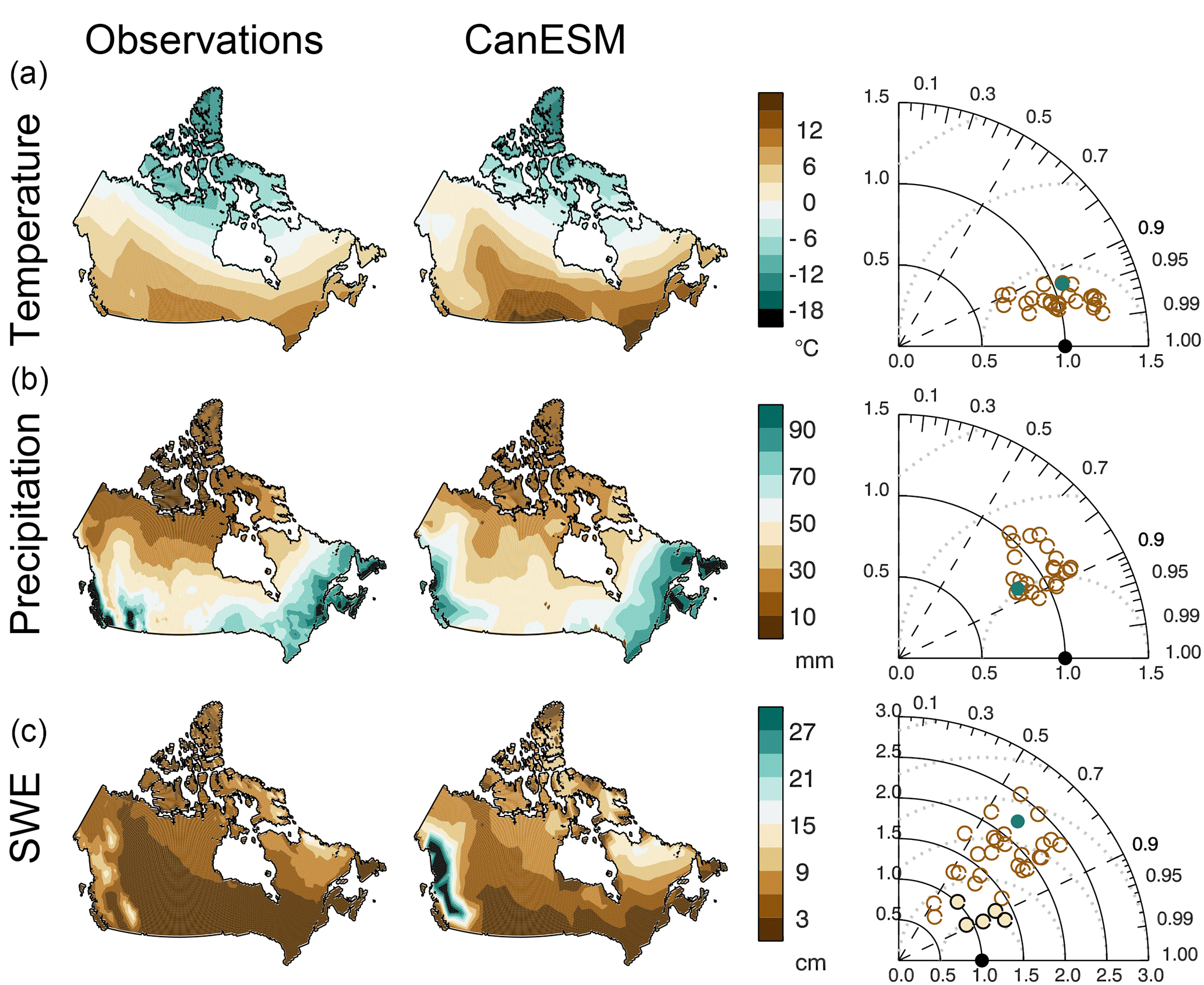
Figure 1 Comparison of simulated Canadian climate in CanESM2 with observations and other climate models for 1981–2005. The left column shows observed January–March (JFM) mean land-surface temperature (a, left panel, HadCRUT4), precipitation (b, left panel, CRU TS3.21), and snow water equivalent (c, left panel, Blended-5 data). The central column shows the same fields as simulated by the ensemble mean of the CanESM2 large ensemble. Observations and the CanESM2 output have been mapped to a common grid that represents the model grid spacing. The right column plots are Taylor (2001) diagrams showing the correlation (related to the polar angle) and standard deviation relative to observations (distance from origin) of the patterns of these variables in observations (black dot), CanESM2 (green dot), and other CMIP5 climate models (brown circles). Models that are closer to the black dot representing the observations have smaller errors (standard error represented by dotted semicircles at intervals of 0.5). In the SWE Taylor diagram (c, right panel), the filled light brown dots compare the individual Blended-5 datasets to the Blended-5 mean.

The use of large initial-condition ensembles has afforded a renewed assessment of the impacts of natural climate variability on recent and projected climatic variability and trends (e.g. Deser et al., 2012; Kay et al., 2015). The CanSISE team designed the CanESM2-LE (e.g. Sigmond and Fyfe, 2016), which consists of four sets of 50 simulations each of CanESM2 that examine the impact of natural and anthropogenic forcings over the period 1950–2100 in the presence of internal climate variability. For each of the five realizations run by CCCma for CMIP5, a new set of 10 simulations is generated by slightly perturbing the atmospheric state at the beginning of 1950, with 10 different perturbations. These 50 realizations are then integrated forward until 2005 with CMIP5 historical forcings (Taylor et al., 2012); from 2006 to 2100, the RCP8.5 CMIP5 scenario is used. The first ensemble set, which applies all available external forcings, will be the one used here. Additional sets of attribution integrations not analyzed here include just historic natural external forcings (solar and volcanic), just historic anthropogenic aerosol forcings, and just stratospheric ozone forcing. Each realization in each set is identical apart from its initial conditions. Thus, the ensemble mean of a given 50-member set is characterized by about a factor of 7 less internal variability than a single realization, and therefore provides a relatively robust estimate of that set's externally forced signal. The distinctively forced ensembles permit attribution of observed climate signals to different external forcings. The CanESM2-LE has been used in several current and ongoing studies (Sigmond and Fyfe, 2016; McKusker et al., 2016; Gagné et al., 2017a; Fyfe et al., 2017; Mudryk et al., 2017; Kirchmeier-Young et al., 2016). We also use similar initial-condition ensembles of the National Center for Atmospheric Research Community Earth System Model 1 (NCAR CESM1; Kay et al., 2015) and the NCAR Community Climate System Model 4 (CCSM4; Mudryk et al., 2013). Other observational sources and modelling results used in this study will be described in the text and figure captions. In what follows, our primary focus is on Canada and the pan-Arctic, placed in the context of northern hemispheric climate.

Besides CanESM2, the other CMIP5 models referenced below are the same as those in Mudryk et al. (2018) (see Table 2 of the paper).

Figure 2 As in Fig. 1, for April–June (AMJ).

3 CanESM2 climatology and trends

3.1 Observed and simulated terrestrial snow climatology

We first evaluate the climatological characteristics of CanESM2's land-surface temperature, precipitation, and SWE for the Canadian land mass. In winter and spring, the distribution of land-surface temperature over Canada is well reproduced in CanESM2, although a warm bias is evident in both seasons (left and central panels of the top rows of Figs. 1 and 2). The Taylor (2001) diagram for land-surface temperature (right panels of Figs. 1a and 2a) shows that CanESM2 compares well to other CMIP5 models (as stated in Sect. 2, the same models and realizations are used in Mudryk et al., 2018) in capturing the spatial pattern and correlation with observations, although the spatial gradients are somewhat stronger than observed for winter (as shown by the distance of the CanESM2 point from the origin in the Taylor diagram), associated with a stronger south-to-north temperature gradient than observed. In JFM precipitation (panel a of Figs. 1 and 2), the general pattern and spatial gradient strength are captured in the model, but there is excessive wintertime precipitation over most of Canada, including the Western Cordillera, sub-Arctic and Arctic, in both seasons. This excessive precipitation contributes towards a bias of excessive SWE over much of western Canada and the Canadian sub-Arctic that is particularly pronounced in spring (panel b of Figs. 1 and 2). CanESM2 SWE has greater spatial variance than the Blended-5 SWE ensemble mean and most of the individual component datasets of the Blended-5 (panel c of Figs. 1 and 2). Generally speaking, the Taylor diagrams in Figs. 1 and 2 suggest that CanESM2 is well within the state of the art of current models for the climate parameters related to seasonal snow cover.

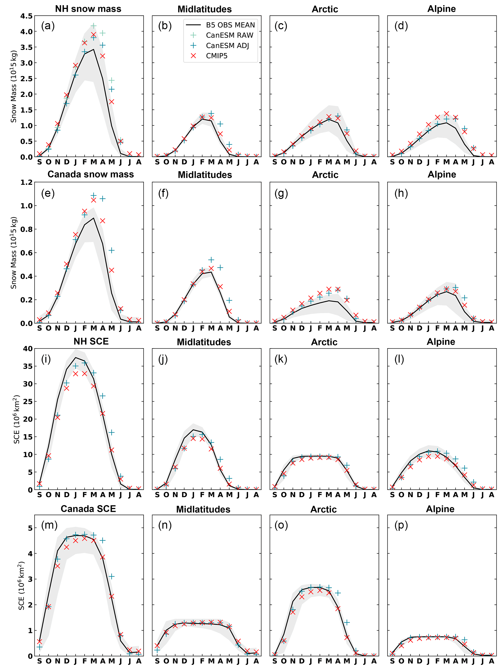
Figure 3 First row: seasonal cycle of Northern Hemisphere 1981–2005 snow mass (in 10¹⁵ kg) for regions defined in Mudryk et al. (2015): midlatitudes, i.e. northern hemispheric non-alpine land regions south of 60^∘ N; Arctic, i.e. non-alpine land regions north of 60^∘ N; and alpine. Grey shading represents the range of Blended-5 datasets, the black curve represents the Blended-5 mean, the light teal points (in panel a) mark the ensemble mean of CanESM2 using its land mask, and the dark teal points mark CanESM2 adjusted to represent the same land fractions as the observational mask from the Blended-5 dataset. The CMIP multi-model mean, adjusted to the observational mask, is show with red x symbols. The legend in panel (b) applies to the figure as a whole. Panels e–h as in panels a–d, but for Canadian land mass only. Panels (i–l) and (m–p) are similar to (a–d) and (e–h), but for snow cover extent in 10⁶ km². The estimate of observed snow cover extent is derived from the Blended-5 SWE dataset using the approach of Mudryk et al. (2017) and is based on a 4 mm SWE threshold for the presence of snow cover; the simulated snow cover extent is based on snow cover fraction directly produced by the models.

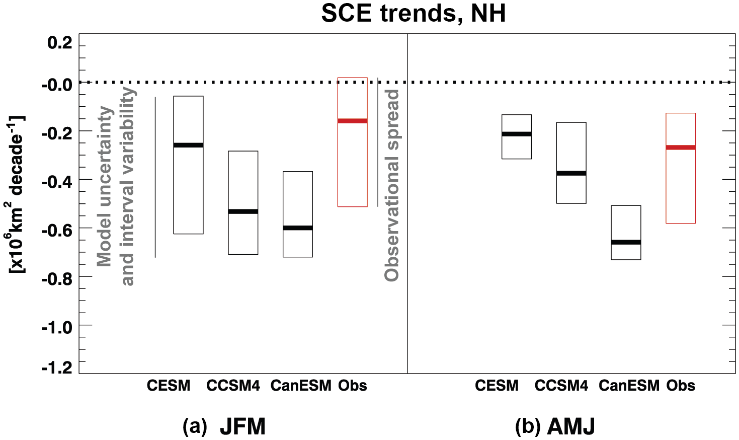
Figure 4 Horizontal bars and boxes show the median and interquartile range of northern hemispheric snow cover extent trends calculated over 1981–2005 period for January–March (a) and April–June (b). Black boxes are used for trends calculated from models (large initial-condition ensembles of NCAR CCSM4, NCAR CESM1, and CanESM2 as labelled), and red boxes are used for trends derived from the Blended-5 SWE dataset (Mudryk et al., 2017). For the models, the boxes indicate the interquartile range (IQR) of trends captured in individual realizations of the ensembles. For the observations, the boxes indicate the IQR of observed trend estimates. Unlike the observational uncertainty, the uncertainty represented for the models is the impact of internal variability on estimated trends. In addition, the IQR of the observations is obtained from only five datasets, which represents a less robust estimate of uncertainty than that from the 30–50 simulated realizations in the large ensembles. Spread from these distinctive sources of uncertainty is indicated schematically by the extent of the vertical grey lines.

Observed SWE climatology, variability, and trends are relatively non-robust compared to variables such as land-surface temperature (Mudryk et al., 2015, 2017) and for this reason we assess some aspects of the spread across the Blended-5 SWE datasets. Individual observational datasets contributing to Blended-5 also show stronger spatial gradients than the Blended-5 mean (circles filled with light brown in the Taylor diagram in Figs. 1c and 2c). This is in part expected because the observational mean will cancel random errors. However, this also suggests that there is considerable uncertainty in the spatial variance, and so it is difficult to assess how realistically spatial variance is captured in CanESM2 and the other CMIP5 models. This observational uncertainty is also evident in the seasonal cycle of total snow mass aggregated for Canada and the Northern Hemisphere, as well as geographic subregions (Fig. 3a–h, grey shading). For example, for the Northern Hemisphere (panel a), the range in Blended-5 estimates of peak snow mass in February is over 50 % of the average and is driven mainly by uncertainty in Arctic (panel c) and alpine regions (panel d). The individual datasets in the Blended-5 product are not shown in Fig. 3, but their characteristics are discussed in Mudryk et al. (2015). The NASA Global Land Data Assimilation System (GLDAS) provides an estimate well below the multi-dataset mean, the MERRA reanalysis dataset typically provides a central estimate, and the maximum estimate varies with region among the remaining three datasets.

After accounting for the considerable observational uncertainty in total snow mass, it is nevertheless possible to assess the realism of CanESM2's simulation. The CanESM2 snow mass for the Northern Hemisphere is plotted as originally available on the model's land grid (light teal points, shown only in Fig. 3a) and as adjusted to reflect the observational mask which is on a finer scale (dark teal points). The adjustment is downward because some of the model's snow mass is located in grid cells that, in reality, are only partially covered by land. The positive bias of CanESM2 relative to the observational mean (Figs. 1 and 2) is evident in the seasonal cycle in snow mass over Canada (Fig. 3e–h), especially in spring in midlatitudes, and reflects a broader northern hemispheric positive bias (Fig. 3a–d). Sospedra-Alfonso et al. (2016a) also find that CanCM4 model that contribute to CanSIPS features a positive springtime SWE bias. For comparison, the CMIP5 multi-model mean over Canada (red x symbols in Fig. 3e–h) does not feature as pronounced a bias. The CMIP5 model range (not shown) spans from the lowest observational estimate to above CanESM2, but CanESM2 is on the high end, especially during spring in the midlatitudes. Our assessment is that, especially in midlatitudes, CanESM2 simulates excessive springtime snow associated with excessive wintertime precipitation building up throughout winter and into spring (middle rows of Figs. 1 and 2).

The seasonal cycle of snow cover extent (SCE) is shown in Fig. 3i–l for North America and Fig. 3m–p for Canada. Here, observed SCE is derived from the Blended-5 dataset by converting SWE to SCE using a threshold of 4 mm; this threshold was tested in Mudryk et al. (2017). For the observational products in the Blended-5 dataset, the relative uncertainty in SCE is generally less than for snow mass. For example, the observational range in peak northern hemispheric SCE in January is about 15 % and is dominated by uncertainty in midlatitude and Arctic regions. A modest positive springtime excess of SCE is evident for CanESM2 for Canada and the Northern Hemisphere. On the whole, observed SCE is better constrained than observed snow mass, and simulated SCE is generally more realistic than simulated snow mass for CanESM2, as well as for the average over the CMIP5 models.

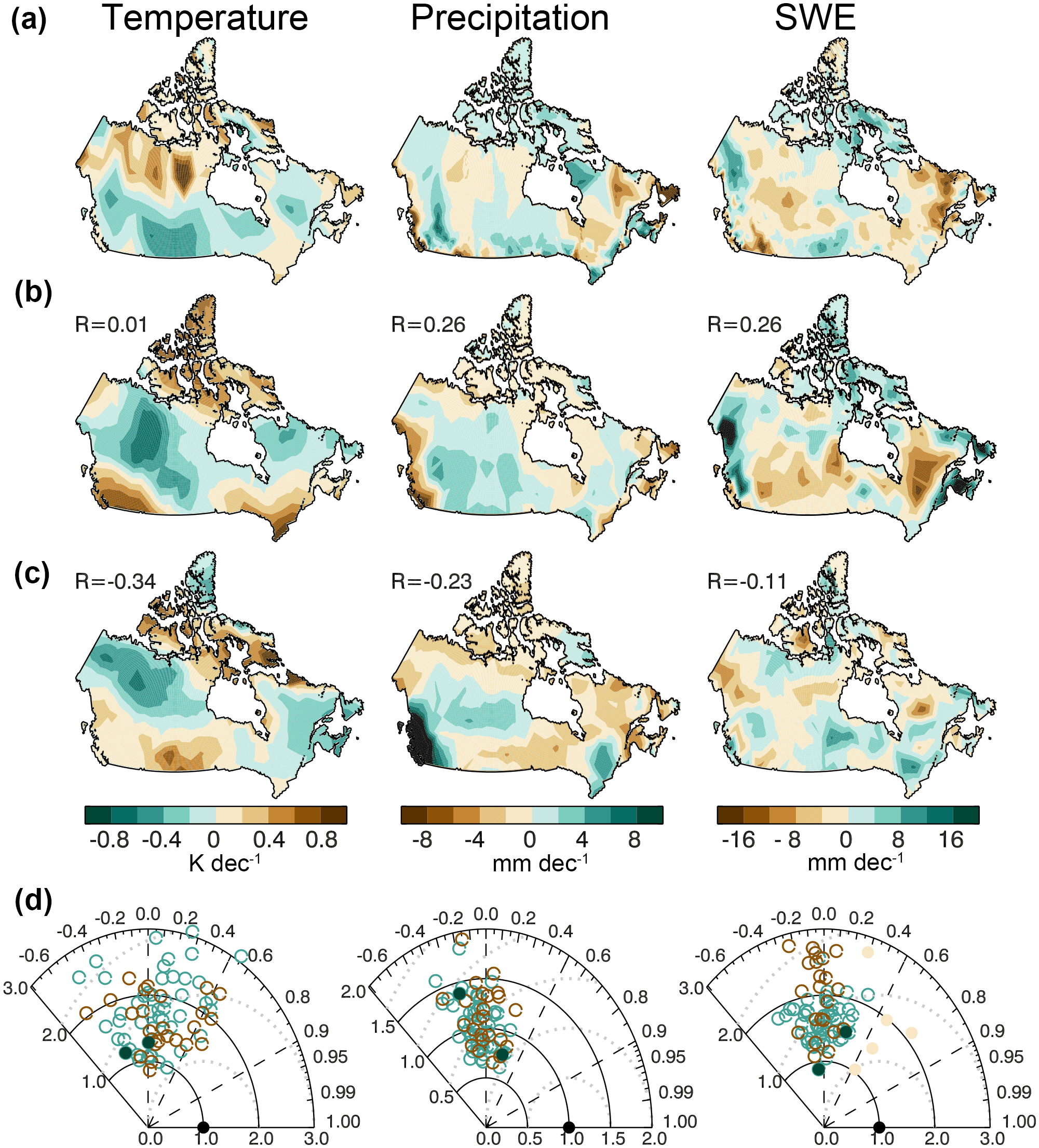
Figure 5 Panel (a) shows the observed 1981–2005 trend over Canada in JFM land-surface temperature, precipitation, and SWE, with the spatial mean of the trend removed, based on the same observational datasets represented in Figs. 1 and 2. Panel (d) shows the Taylor diagram of individual realizations of CanESM2 (teal) and CMIP5 (brown). The Taylor diagram for SWE also includes individual Blended-5 observations (light brown). Panels (b) and (c) show the land-surface temperature, precipitation, and SWE trends for the best match and worst match realizations as defined in the text. The best and worst match realizations are shown as filled circles in the Taylor diagrams. Note that the realizations represented are the same in this figure and in Fig. 6.

3.2 Observed and simulated trends in terrestrial snow

A standard target for snow process analysis in climate models is trends of SCE, which are strongly temperature controlled (e.g. Brutel-Vuilmet et al., 2013; Mudryk et al., 2017). Assessing the ability of models to capture these trends needs to account for natural variability, forced variability, observational uncertainty, and inter-model differences. We show in Fig. 4a and b the trends in SCE derived from the Blended-5 dataset for the Northern Hemisphere in January–March and April–June. In both seasons, there is a spread of observed seasonal snow cover reduction estimates from 0.0 to −0.5 million km² per decade in winter (based on a simple interquartile range for this small number of observational datasets) and from −0.1 to −0.6 million km² in spring. The red horizontal line in the box plot represents the median over the Blended-5 datasets. Over the 25-year observational period, the trends correspond to an approximate snow loss that is at most 4 % of JFM SCE and in the range of 5–40 % of AMJ SCE. The range of trends from the CanESM2-LE, NCAR CESM1, and NCAR CCSM4 suggests that internal variability alone provides an uncertainty range of about 0.5 million km² per decade. Assuming internal variability is realistic in the models, this is the limit of precision we can expect in assessing recent trends. CanESM2 consistently produces greater snow loss than NCAR CCSM4 and CESM1, especially in AMJ. We conclude that all the models displayed fall within wintertime snow retreat estimates, that NCAR CCSM4 and CESM1 overlap with estimates of observed snow retreat in spring, but that CanESM2 exhibits more spring snow retreat than our best estimate of the observations. This excessive snow retreat is associated in part with excessive global warming in the model mentioned in Sect. 2 (Mudryk et al., 2017).

Figure 6 A similar analysis to Fig. 5 but for AMJ. Panels (a) and (d) represent AMJ trends, and (b) and (c) represent the same best match and worst match realizations from Fig. 5, but with AMJ trends displayed.

A more challenging target for the purpose of simulation and attribution of climate change on a regional scale is the spatial pattern of observed climate fluctuations in recent decades. Acknowledging the overall biases noted above, we concentrate our analysis on the response patterns with spatial means removed. We first show the wintertime 1981–2005 land-surface temperature trend pattern with the spatial mean removed in the left panel of Fig. 5a. This represents a predominantly positive meridional gradient of land-surface temperature change from southern to northern Canada, reflecting wintertime Arctic amplification of warming. The same field in individual realizations of CESM1 and CanESM2 has a spatial correlation in the range of −0.6 to +0.6 (Taylor diagram in the left panel of Fig. 5c), suggesting that these patterns are affected by significant internal variability (Deser et al., 2012). There are more realizations with positive than negative spatial correlation in winter land-surface temperature trend patterns, which is consistent with the anticipated effect of anthropogenic forcing. Wintertime land-surface temperature trends systematically show greater spatial variance than the estimated warming pattern from the single observational land-surface temperature dataset employed here. This could be related to stronger (more negative) meridional gradients in land-surface temperature and its trends in the models compared to the observational dataset. Springtime land-surface temperature trend patterns (left panel of Fig. 6a) feature anomalously negative changes in the Canadian prairie regions and positive changes around the coastal regions. It is harder to find realizations in the spring that correspond to the observed pattern (left Taylor diagram in Fig. 6d), and spatial variance of the land-surface temperature trends appears to be biased high as in winter. For precipitation, there is little evidence of consistent pattern matching between the observations and individual realizations, for winter or spring (middle column of panels a and d of Figs. 5 and 6). For SWE spatial patterns (right column of panels a and d of Figs. 5 and 6), the structural details of the trend maps are also not readily found in the models compared to the mean of the Blended-5 SWE. Compared to the ensemble mean of the Blended-5 observations, the simulations show greater spatial variance in SWE trends, but this is partially due to smoothing of spatial structure in observational errors, as is shown by the scatter of SWE trends by individual contributors to the Blended-5 dataset (light brown circles in Taylor diagrams).

It is possible to find individual realizations in the CanESM2-LE that match either fairly well or fairly poorly with observed trends. In panel b of Figs. 5 and 6, we show for the two seasons of JFM and AMJ, respectively, the land-surface temperature, precipitation, and SWE trends for the best all-round match realization, which is a single realization with the greatest average pattern correlation across the three fields (land-surface temperature, precipitation, and SWE) and the two seasons of JFM and AMJ. The spatial pattern correlation coefficient of each field with its observational counterpart is labelled. Plotted in Figs. 5c and 6c is the worst all-round match realization, which is the single realization with the least (most negative) pattern correlation. The best match realization exhibits tradeoffs across fields, for example in the ability to represent the structured pattern of springtime precipitation change (r=0.38 for the middle panel of Fig. 6b) versus wintertime land-surface temperature change (r=0.01 for the left panel of Fig. 5b). The worst match case exhibits a similar range of correlations, on the negative side, and generally looks quite different from the best match case. This preliminary analysis of intra-ensemble variability suggests limits on how much regional-scale information about changes for snow cover and related climate variables can be extracted from ESMs. The key point is that caution is needed in judging a model on its ability to reproduce spatial patterns of trends in SWE and related climate parameters, even on these multidecadal timescales.

Figure 7 Column (a) shows the multimodel mean of CMIP5 trends over the 1981–2005 historical period for JFM land-surface temperature, precipitation, and SWE. Column (b) shows the corresponding multi-realization mean for the CanESM2 large ensemble. Unlike Figs. 5 and 6, the spatial mean of the trend has not been removed.

The spatial pattern of CanESM2 land-surface temperature and precipitation trends is generally representative of that found in individual realizations of the CMIP5 datasets, in the sense that the individual realizations of CanESM2 and other CMIP5 models have positive pattern correlations with the CMIP5 multi-model mean (Taylor diagrams not shown). Consistently, the CMIP5 multimodel mean of the land-surface temperature and precipitation trends are generally similar to the CanESM2 ensemble mean (winter example shown in the top two rows of Fig. 7; note that in Fig. 7 the spatial mean of the patterns is not removed in order to allow comparison of the overall responses in CanESM2 to CMIP5). However, for SWE, we find CanESM2's pattern is typically opposite that of individual realizations from other models in CMIP5 (not shown) as is also evident in the ensemble mean (bottom row of Fig. 7). In particular, CanESM2 shows a strong positive trend in the Western Cordillera and a weaker positive trend in Southern Ontario and eastern Canada in both winter (Fig. 7) and spring (not shown), whereas a reduction of SWE is found in these regions and seasons in CMIP5.

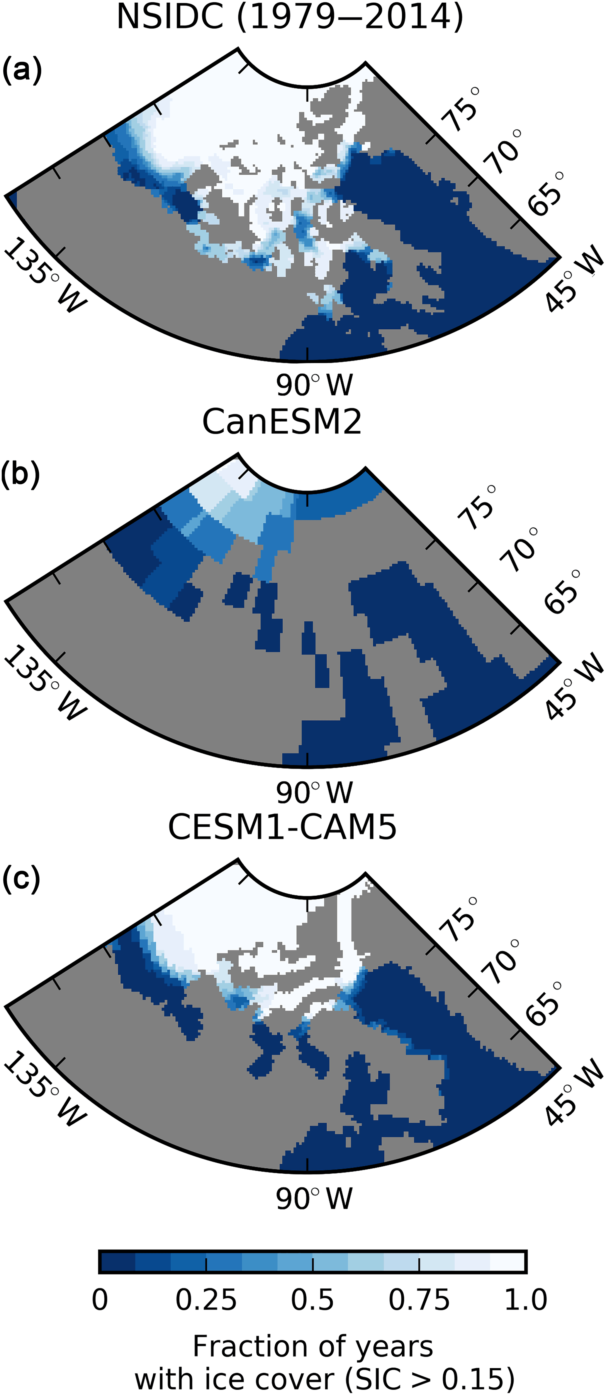
Figure 8 (a) Fraction of years (1979–2014) with September sea ice cover (sea ice concentration > 0.15) for the NSIDC passive microwave product on an EASE 25 km grid. (b) as in (a) but for the CanESM2 model, remapped using a nearest-neighbour remapping. (c) as in (b) but for the CESM1-CAM5 model. The grey shading indicates the land–sea mask for each dataset. The NCAR CESM1 CICE grid provide a rough indication of how geographical features of the Canadian Arctic, such as the Canadian Arctic Archipelago, might be resolved in future configurations of CanESM2. Also evident is the low September sea ice extent bias in CanESM2.

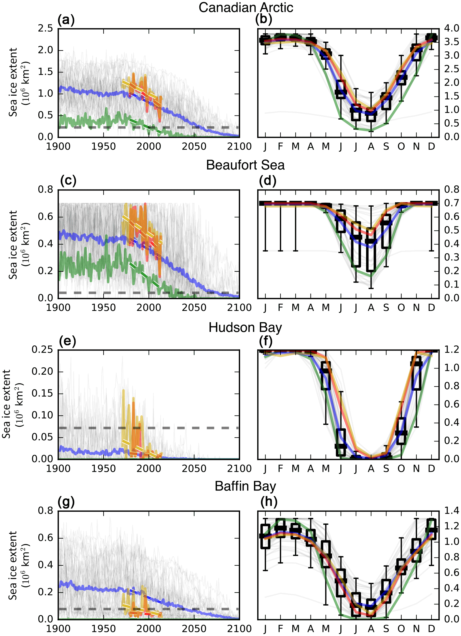
Figure 9 (a) September sea ice extent (sea ice concentration larger than 0.15) for the Canadian Arctic (defined by the Canadian Ice Service Data Archive (CISDA) domain). The CanESM2 model (green), CISDA (yellow), National Snow and Ice Data Center (NSIDC, red), and the multi-model mean (blue) are shown with their 1979–2013 trends. Individual models are shown in light grey. (b) The Canadian Arctic seasonal cycle for 1979–2013. Box plots were added to describe the inter-model spread (whiskers are 5th and 9th percentiles). Panels (c–d), (e–f), and (g–h) are the same as panels (a) and (b) but for the Beaufort Sea, Baffin Bay, and Hudson Bay, respectively. In panels (e) and (g), the CanESM2 curve is close to zero. Sea ice amounts are scaled to account for the fraction of ocean present in the CanESM2 land–sea mask (Laliberté et al., 2016).

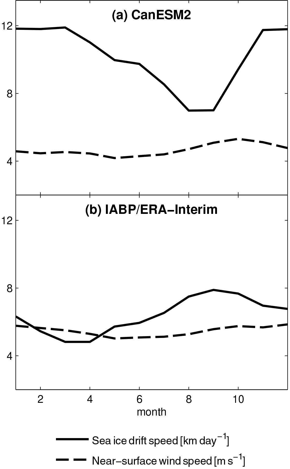
Figure 10 (a) Seasonal cycle of Arctic average sea ice drift speed (solid, in units of km day⁻¹) and near-surface wind speed (dashed, in units of m s⁻¹) from a historical run of CanESM2 averaged over 1979–2005. The spatial domain used for the calculation is the region north of 68^∘ N for longitudes east of 103^∘ E and west of 124^∘ W and north of 79^∘ N at all other longitudes, excluding grid points within 150 km of a coastline. This focuses on regions of year-round drifting ice and excludes landfast ice. (b) as in (a) but using non-gridded drift speed measurements from the International Arctic Buoy Programme (solid; Tschudi et al., 2016) and near-surface wind data from ERA-Interim (dashed; Dee et al., 2011).

3.3 Canadian Arctic sea ice in CanESM2

Turning to sea ice, we recall that it is well established that summertime Arctic sea ice area or extent is biased low in CanESM2 (Stroeve et al., 2012; Merryfield et al., 2013a; Laliberté et al., 2016). We thus focus a limited amount of additional analysis on sea ice in the Canadian sector. The established low bias is borne out in the Canadian Arctic sector (Fig. 8a–b), where CanESM2 has less than half of the observed sea ice coverage in the Beaufort Sea–Arctic Ocean sector. Further limiting the utility of regional sea ice analysis with this model is the moderate spatial resolution of the model and its associated land–sea distribution, particularly in the Canadian Arctic Archipelago (Fig. 8a–b). The summertime sea ice extent is among the lowest of all CMIP5 models in the Canadian Arctic as a whole. In Canadian Arctic regions, summertime sea ice extent is biased low in the Beaufort Sea and is practically zero in Hudson Bay and Baffin Bay (Fig. 9, left column). This bias contributes to the outcome that the sea ice reaches nominally ice-free summertime conditions at times comparable to present-day in CanESM2. The bias is evident throughout the seasonal cycle in most regions (Fig. 9, right column), with the exception of Baffin Bay, although not as extreme relative to other models in other seasons as it is in summer. In this respect, the quality of simulation in CanESM2 is not as good as that of other ESMs such as NCAR CESM1 (Fig. 8c), which provide a better baseline for regional sea ice studies in terms of both climatology and land–sea distribution.

Process investigations of sea ice by CanSISE include a focus on the relationship between sea ice drift and Arctic winds, since realistic sea ice dynamics are crucial for accurate representation of sea ice (Notz, 2012). International Arctic Buoy (IABP) Programme measurements (Tschudi et al., 2016) show that sea ice drift speed peaks in September, when sea ice is thinnest (Fig. 10b), and not at the time of peak wind speed in December. However, in CanESM2, the peak sea ice drift speed occurs in November and is more in phase with the seasonal cycle of near-surface wind speed. Other models in the CMIP5 archive that have more modern sea ice components are able to reproduce more closely the observed seasonal cycle of sea ice drift speed (Neil F. Tandon, personal communication, 2018). These results provide strong motivation to transition to a modelling system with improved sea ice and related processes in the Arctic.

4 Snow- and sea-ice-related forecast performance and development of CanSIPS

Operational seasonal forecasts based on coupled global ocean–atmosphere models have been produced for about two decades internationally (Stockdale et al., 1998) and in Canada (by CanSIPS) since 2011. Over this period the main emphasis has been on predicting seasonal meteorological variables describing near-surface temperature, atmospheric circulation, and precipitation, as well as sea-surface temperatures, since these are a major driver of seasonal climate variations. Potential has also existed for such systems to usefully predict additional variables, including snow and sea ice, particularly as the sophistication of the models and the methods used to initialize them have increased. With respect to the cryosphere, however, such capabilities have received little attention until relatively recently compared to other areas of focus in seasonal prediction (e.g. Blanchard-Wrigglesworth et al., 2011; Sigmond et al., 2013; Guémas et al., 2016).

4.1 Characteristics of CanSIPS related to seasonal forecasts of terrestrial snow

Research carried out under CanSISE examined the ability of CanSIPS both to realistically initialize SWE and to predict future SWE variations (Sospedra-Alfonso et al., 2016a, b). This was the first study of snow in an operational seasonal forecast system. Regarding seasonal prediction of snow by CanSIPS, anomaly correlation skill for wintertime SWE is high at short lead times and remains statistically significant (greater than 0.3) at lead times of at least 6 months for certain regions (Fig. 11), which suggests potential for practical utilization of such forecasts. Two primary sources of potential predictability (PP, defined as the ratio of “signal” variance describing interannual variability of ensemble means to total variance consisting of the sum of “signal” and “noise” components) and skill in CanSIPS forecasts of SWE have been identified (Sospedra-Alfonso et al., 2016a, b). The first, which is most important at short lead times, is the demonstrated ability of CanSIPS to provide realistic initial values for SWE, combined with the natural tendency for SWE anomalies to persist throughout the snow season in regions where winter land-surface temperatures remain below freezing, so that the snowpack accumulates until the onset of spring melt. The second main source of PP and skill, which becomes increasingly prevalent at longer lead times, is the ability of CanSIPS to predict future climatic conditions such as land-surface temperature and precipitation anomalies which influence snow accumulation and melt. A large part of this type of predictability and skill arises from ENSO, which strongly influences winter climate in North America and is skillfully forecast by CanSIPS up to a year in advance.

The value of skillful seasonal forecasting of snow in turn depends on process representation and initialization at the land surface. For example, Ambadan et al. (2015) have investigated the impact of initialization of SWE, soil liquid water, and soil frozen water on PP of springtime surface air temperature in the CanSIPS system (Fig. 12). Realistic initialization of these variables enhances PP by as much as 30 % in terms of variance explained within the PP framework. This shows that it is important to regard snow initialization in the broader setting of land-surface initialization and that there is evidence for quantitative improvement in regional predictability as more observational information on the state of the land surface is brought into the prediction system. Current operational practice in CanSIPS uses observed atmospheric forcing to bring the land surface (including soil moisture and snow cover) into a realistic state. Although this procedure performs reasonably well for snow (within observational uncertainty), potential remains for improving the initialization and forecasting of snow and other land variables by assimilating observation-based land data directly in real time.

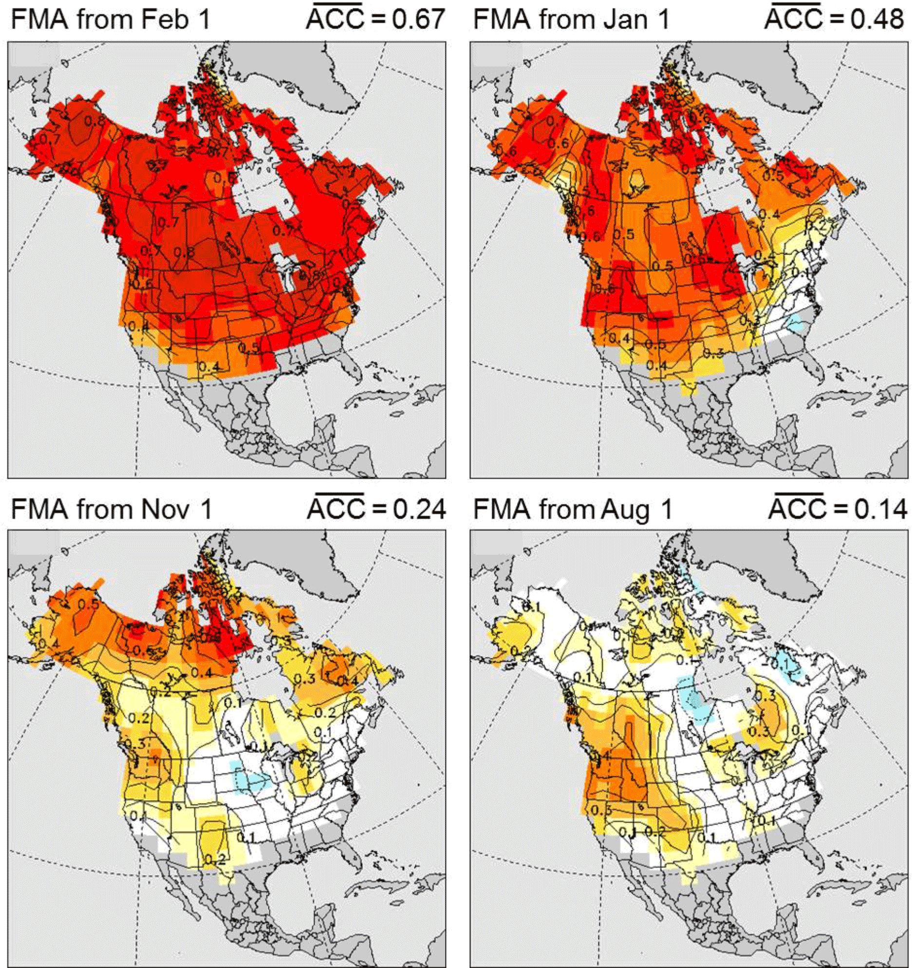
Figure 11 Anomaly correlation coefficient (ACC) skill for February–April (FMA) SWE of 1981–2010 CanSIPS hindcasts initialized at the start of February and the preceding January, November, and August (lead times of 0, 1, 3, and 6 months, respectively). The Blended-5 dataset of Mudryk et al. (2015) is used for observational verification. The contour interval is 0.1, and the overbars denote spatial averages of ACC over areas of North America having seasonal snow cover.

Figure 12 Impact on the square of the anomaly correlation coefficient of initialization of (a) SWE, (b) frozen soil water, and (c) liquid soil water on springtime forecasts of land-surface temperature at 45-day lead. Red colours indicate increase and blue colours decrease of the potential predictability (an idealized model based estimate of potential forecast skill). Based on Ambadan et al. (2015).

Blending different sources of data from highly uncertain observations has led to improved characterization of the forecast skill of the CanSIPS system. Figure 13 shows the degree of agreement between SWE forecasts from CanSIPS and several SWE products over Canada (similar results are found for other regions). The degree of agreement is measured as the anomaly correlation coefficient for a 1-month forecast (with lead 0 from initialization). The five datasets are the Blended-5 dataset (blue) and four individual datasets including two components of the Blended-5 dataset. Even though all observational datasets are being compared to the same forecast, it is the Blended-5 dataset, capturing the mean of several observational datasets, that agrees best with the forecast. It is clear that improving verification datasets through blending, which can be reasonably expected to lead to cancellation of independent errors in observational estimates, impacts assessed agreement with the forecast. To reiterate, in this case, improved calculated skill is derived from an apparent improvement in the quality of the verification data and not an improvement of the forecast (Sospedra-Alfonso et al., 2016b). Whether or not such improved consistency might be found for the prediction of other quantities, the broader point is that there is a need to ensure that verification data are continually updated in order to fairly compare predictions to the best available data (Massonet et al., 2016).

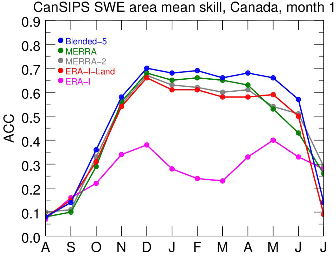
Figure 13 Anomaly correlation coefficient (ACC) averaged over Canada for first-month CanSIPS forecasts of SWE, verified against several observation-based datasets including Blended-5 (blue), MERRA (green), MERRA-2 (grey), ERA-Interim Land (red), and ERA-Interim (magenta); the MERRA and ERA-Interim Land are components of Blended-5. Blended-5 shows the best agreement with the forecast, suggesting a strong influence of observational dataset on evaluation of forecast performance.

Recent research in snow analysis and observational datasets is expected to support operational improvements in CanSIPS and hence in ECCC's operational prediction capacity. For example, CanSISE work has led to new efforts to develop an operational real-time snow amount forecast for the coming months, which could be used in several impacted sectors such as outdoor recreation, water resource planning, and agriculture (Fig. 14, snow amount forecast shown as above and below normal SWE amounts). In this successful proof of concept, we note satisfactory general agreement with the MERRA analysis, which is independent of CanSIPS and is itself subject to some uncertainty. This indicates promise for this new forecast product, while highlighting issues of observational uncertainty addressed in part by our recent research.

4.2 Sea ice forecasting with CanSIPS

Much as for snow, the ability of global climate model-based seasonal forecasting systems to predict sea ice has also received little attention until recently, although such assessments have now been carried out for several systems (Guémas et al., 2016). In the area of sea ice prediction, CanSIPS hindcasts, despite some of the simulation deficiencies described above, have demonstrated skill in seasonal predictions of sea ice (e.g. Sigmond et al., 2013; Merryfield et al., 2013b). While these prior studies have focused on forecast skill of area-integrated quantities such as sea ice area, recent work (Sigmond et al., 2016) has also shown significant forecast skill of more user-relevant sea ice metrics such as the first calendar date that sea ice melts (retreat date; Fig. 15a–c) or freezes up (advance date; Fig. 15d–f). Advance dates are skillfully predicted at lead times of 5 months on average (3.3 months for detrended anomalies) and retreat dates at lead times of 3 months (2.2 months for detrended anomalies). For retreat dates, the main source of forecast skill is persistence, while advance date predictions benefit from predictable ocean temperatures.

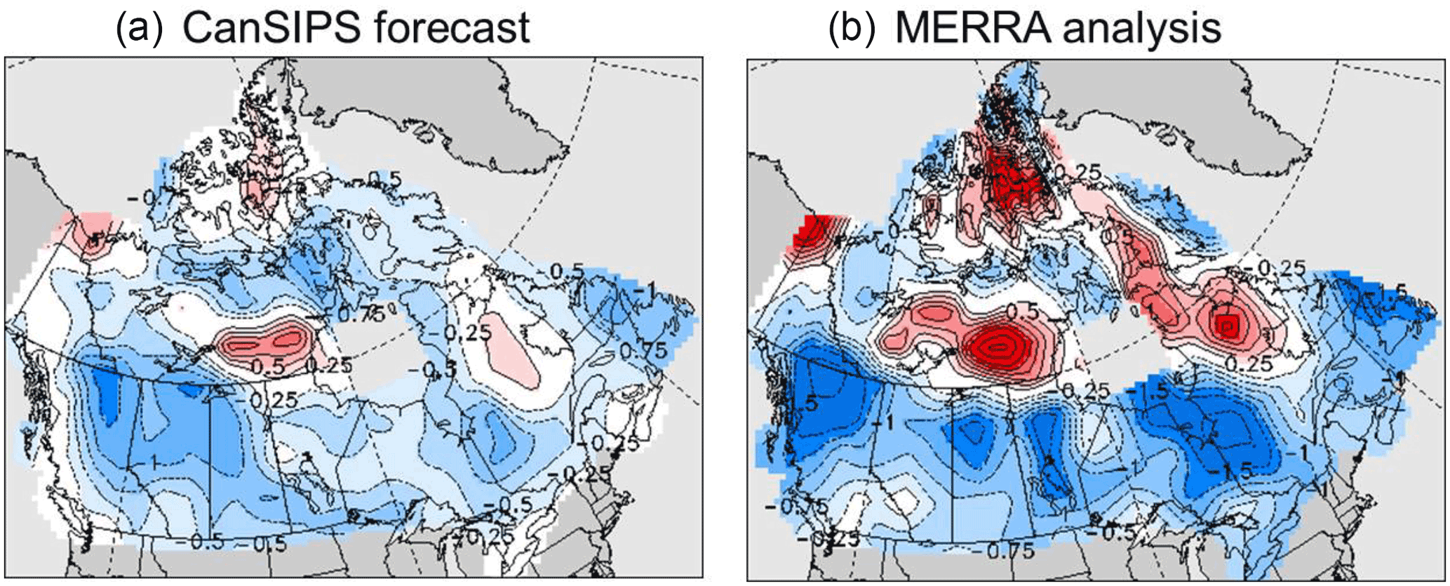
Figure 14 Real-time CanSIPS forecast of standardized anomalies of monthly-mean SWE for January 2016 (a), initialized at the end of the preceding month, compared to the MERRA analysis for the same period (b). The contour interval is 0.25, and anomalies are relative to a 1981–2010 base period.

Figure 15 Maximum lead time at which CanSIPS skillfully predicts retreat and advance dates (defined as the calendar date at which sea ice concentration first drops below or exceeds 50 %) for total anomalies (first column), detrended anomalies (second column), and a detrended persistence forecast based on persisting the observed initial sea ice concentration anomaly. The numbers in the top right corner of each panel indicate the Arctic average maximum lead time (in months). From Sigmond et al. (2016).

Sea ice predictability is also assisted by persistence of sea ice thickness (e.g. Chevallier and Salas-Mélia, 2014), but CanSIPS does not take advantage of this in that it currently employs an initialization method that uses only climatological sea ice thickness (SIT) information. Since real-time SIT observations are limited, Dirkson et al. (2015, 2017) have developed several statistical models of varying complexity for initializing SIT in operational predictions. These are based on predictors available in real time together with historical SIT values represented by the pan-Arctic Ice and Ocean Modelling System, or PIOMAS (Zhang and Rothrock, 2003), which is frequently used as a reference dataset for SIT due to the sparseness of historical SIT observations. The first such model (known as “SMv1”), described in Dirkson et al. (2015), uses a statistical approach to find an optimal combination of sea ice concentration and sea level pressure information to provide useful sea ice thickness information. While this model reduces temporal- and spatial-mean absolute errors in the SIT initial conditions by 48 % relative to the original CanSIPS initialization (when validated against PIOMAS SIT values) and shows consistent skill estimating ice volume in all months, much of this improvement in skill emerges from a more accurate representation of local negative trends in SIT. Two additional statistical models, “SMv2” and “SMv3”, that improve on SMv1 with respect to interannual variations in SIT anomalies are described in Dirkson et al. (2017), and seasonal sea ice volume from SMv3 is compared to that from CanSIPS initial conditions in Fig. 16. Seasonal forecasting experiments using these SIT initial conditions demonstrate general improvement forecasting both pan-Arctic sea ice extent and local sea ice concentration compared to the current operational system, with most significant improvements afforded by initializing with either SMv2 or SMv3 (Dirkson et al., 2017).

Figure 16 Time series of seasonally averaged sea ice volume over the period 1981–2012, in units of 10³ km³ for the PIOMAS sea ice thickness analysis (which assimilates observations) (black), the SMv3 statistical model of Dirkson et al. (2017) (red), and CanSIPS initial conditions (cyan). The CanSIPS system as originally configured incorporates no information about recent sea ice thinning and thus misses the recent downward trends of sea ice volume.

5 Conclusions

We have assessed characteristics of snow, sea ice, and related climate parameters in Environment and Climate Change Canada's (ECCC) Earth system model (ESM) CanESM2 and seasonal to interannual climate-prediction system CanSIPS, with a focus on the Canadian sector of the Northern Hemisphere. This assessment is intended to provide a baseline for future versions of the models with respect to these important societally relevant climate parameters. It has highlighted the application of the Blended-5 multi-source SWE (Mudryk et al., 2015) and the CanESM2-LE of climate simulations. In addition, it has highlighted new developments in sea ice, snow, and related climate parameter prediction on seasonal timescales. We summarize our key findings:

• The CanESM2 simulation of climate parameters over the Canadian land mass closely tied to snow – land-surface temperature and precipitation on land in cold regions – lies well within the range of currently available international models. There is considerable disagreement among observational datasets on the amount and geographical structure of SWE in the satellite era. The CanESM2 simulation of SWE performs as well as available international models in this area. Even accounting for this observational uncertainty, however, there is a bias towards excessive seasonal snow cover and unrealistic spatial distribution of SWE in the spring over the Canadian land mass and over the Northern Hemisphere as a whole. Excessive precipitation over the Canadian land mass contributes to this bias.

• Accounting for observational uncertainty, CanESM2 simulates a greater retreat of springtime snow over the satellite era than most of the available observations assessed here and other models that include large initial-condition ensembles. The spatial pattern of the observed temperature, precipitation, and SWE trends is strongly influenced by internal variability. This makes it difficult to assess the model-simulated patterns of change in the variables we have examined. Nevertheless, Western Cordillera trends in SWE in CanESM2 represent a recent increase that is opposite to those found in typical CMIP5 models.

• Previously identified biases towards low Arctic sea ice extent are also reflected in regional biases: in Hudson's Bay and the Canadian Beaufort Sea sector, the sea ice extent is biased low and this undermines projections of when regional sectors of the Arctic will be ice-free. In the current system, there are tradeoffs related to the resolution of geographical features in the CanESM and CanSIPS systems that impact both the snow and sea ice simulations. This provides an urgent area of improvement for future model development.

• Recent work suggests promising potential for seasonal forecasting of snow, sea ice and related climate parameters using CanSIPS. For example, accurate initialization of frozen and liquid soil water, in addition to improved SWE representation, might lead to significantly improved seasonal temperature forecasts. Furthermore, the Blended-5 example shows that accounting for observational uncertainty can lead to better understanding of forecast quality. This result suggests initialization could also be improved in this manner. This and related work has stimulated the development of ECCC's first experimental seasonal snow amount forecast product.

• Despite biases in the sea ice simulation, it is possible to develop potentially useful new seasonal forecast products for sea ice advance and retreat. In addition, implementing sea ice thickness initialization using indirect statistical predictors of thickness can improve sea ice forecasts compared to the current methodology. Motivated by the promising research results, improved sea ice thickness initialization (as initially explored by Lindsay et al., 2012, and Day et al., 2014) is being considered for implementation in the CanSIPS system.

Further improvements in the CanSIPS and CanESM climate prediction and projection capacity for snow, sea ice, and related climate variables also hinge on assessing model process representation in more depth. For example, critical to capture accurately is the snow albedo feedback process, which governs the seasonality of snow cover and land-surface temperature and hydroclimatic responses to climate change (Qu and Hall, 2007, 2014; Hall et al., 2008; Thackeray et al., 2015; Thackeray and Fletcher, 2016). Thackeray et al. (2015) show that CanESM2 places among the best CMIP5 models for all regions in terms of the overall simulation of snow cover fraction and snow-covered surface albedo. Further progress in this kind of process representation will be achieved in part through internationally coordinated intercomparison efforts associated with CMIP6, including the Land Surface, Snow and Soil Moisture Model Intercomparison Program (LS3MIP; van den Hurk et al., 2016) and the Earth System Model Snow Intercomparison Project (ESM-SnowMIP). Besides ongoing work on sea ice mechanics and its relationship, through wind driving, to sea ice drift, CanSISE research is also currently characterizing snow cover on sea ice in models and observations, which also serves as a potential source of model error in the timing and amplitude of sea ice growth and melt.

CanSISE demonstrates the utility of entraining a network of researchers bridging observational and modelling communities to focus on a related set of processes in evaluation of Earth system models and climate-prediction systems. The results suggest that there can be several benefits to updated multi-source observational datasets for climate prediction, monitoring, and assessment. Our focus in this paper has been on recently produced multi-source snow observational datasets, but our results suggest that there are benefits of multi-source temperature, precipitation, and sea ice datasets that follow a similar approach (Massonet et al., 2016). We have articulated the tradeoffs involved in constraints on CanESM2's resolution in light of limitations of available advanced computing resources. Running the model at 2^∘ latitude–longitude permits the creation of the CanESM2-LE set, but can entail under-resolution of key features of interest in applications, such as the Canadian Arctic Archipelago's channels and islands. We suggest that similar large ensembles be considered based on future model versions, accounting for these tradeoffs, and being complemented by ECCC regional climate model simulations (e.g. Scinocca et al., 2016).