Influence of snowpack properties and local incidence angle on SAR signal depolarization: a mathematical model for high-resolution snow depth estimation

Recently, Dual-Polarimetric Synthetic Aperture Radar (SAR) has been shown to be effective for large-scale snow cover monitoring, but it faces significant challenges when applied to finer resolutions, which are crucial for applications such as avalanche forecasting. In this study, we propose a novel mathematical model to retrieve snow properties from Sentinel-1 SAR data, leveraging variations in the Dual-Polarimetric Radar Vegetation Index (DpRVI_c). We introduce the Snow Index SAR (SIsar), which approximates variations in signal depolarization occurring within the snowpack. Our study, conducted in the Central Italian Alps, reveals a strong correlation between the SIsar index and the snowpack height, enabling accurate snow depth estimation. We also demonstrate the significant impact of the local incidence angle on signal depolarization during the accumulation season. Based on this, we derive a mathematical correction for the incidence angle, whose inclusion in the model reduces snow depth estimation errors by approximately 39 %. The model validation conducted in Tromsø (Norway) and in Davos (Switzerland) confirms its applicability beyond the calibration area, with a root mean squared error (RMSE) of 30.7 cm and a mean absolute error (MAE) of 24.3 cm in Tromsø, and a RMSE of 22.4 cm and a MAE of 18.1 cm in Davos. These findings enhance our understanding of dual-polarimetric Sentinel-1 SAR data sensitivity for high-resolution snow monitoring, providing valuable insights for avalanche forecasting and hydrological applications.

1 Introduction

Snow, in addition to being a complex meteorological phenomenon, represents one of the main resources of the mountain environment, and it is well-established that more than one-sixth of the Earth's population relies on glaciers and seasonal snow for their water supply (Barnett et al., 2005). Moreover, this water source is released gradually during the spring and summer season, filling rivers and lakes, allowing the production of hydroelectric power (80 % of Alpine waterways are exploited by hydroelectric power plants) and, above all, renewing the groundwater reserves essential for drinking water supply and agriculture (Soncini and Bocchiola, 2011). Furthermore, snow monitoring is critically important for avalanche forecasting, indeed snow avalanches are among the most significant hazards in mountain regions, causing approximately 100 fatalities in Europe alone each winter (EAWS, 2025). While for environmental purposes the study of snow at the large-scale is essential (i.e., from a single mountain range to the entire globe), for avalanche forecasting purposes there is more interest in the distribution and properties of the snowpack at the small-scale (i.e., from an individual slope to a single mountain massif; Mariani et al., 2023, 2024).

In recent years, satellite remote sensing has become a fundamental tool for monitoring snow cover properties at the large-scale, particularly in remote regions lacking monitoring stations (Awasthi and Varade, 2021). One of the most important snow properties that can be monitored using remote sensing techniques is the snowpack height (HS). In this study, we propose a new mathematical model for estimating HS using dual-polarimetric Synthetic Aperture Radar (SAR) data, which corrects biases inherent in previous methods, thereby improving the retrieval of HS at the small-scale.

Initially, optical satellite data with medium or high resolution, such as Moderate-Resolution Imaging Spectroradiometer (MODIS), Advanced Very High-Resolution Radiometer (AVHRR), and Sentinel-2, served as the primary spaceborne data sources for monitoring snow cover extent and surface properties (Feng et al., 2024). However, optical imaging has significant limitations: it cannot provide information under cloud cover or during nighttime and is sensitive only to the surface of the snowpack. To overcome these limitations, the use of SAR data has been widely explored since the first pioneering studies on microwave interaction with snow reported a certain sensitivity on snow as a volume (Ulaby and Stiles, 1981; Kendra et al., 1998; Tsai et al., 2019).

The interaction of electromagnetic waves with snow is a result of the geometrical structure of the snowpack and of the electromagnetic properties of its single components: air, ice, water vapor, and, when the snow is wet, liquid water. The basic electromagnetic properties are thus the relative dielectric constants of ice and liquid water, and their geometrical distribution in the snow cover (Tiuri et al., 1984; Mätzler, 1987). The presence of a certain liquid water content in the snow strongly influences the amount of backscattered signal, making wet snow retrieval one of the primary applications of SAR related to snow monitoring (Picard et al., 2022). Key contributions in wet snow retrieval include the works of Nagler and Rott (2000) and Nagler et al. (2016). Additionally, SAR satellites are increasingly used to detect avalanche deposits, providing crucial data for avalanche forecasting (Kapper et al., 2023). The sensitiveness of microwave instrument to snow volume variations also depends on the microwave frequency (Strozzi et al., 1997). At the frequencies commonly used for snow monitoring in SAR missions, such as X-band and C-band, the radar signal penetrates a dry snowpack (i.e., a snowpack without liquid water), reaching the underlying soil and leading to surface backscatter, which predominantly contributes to the total received signal in both co- and cross-polarizations (Wiesmann et al., 2007; Awasthi and Varade, 2021). However, the snow volume tends to depolarize the signal, leading to a certain backscatter increase, compared to bare soil, in cross-polarization (Kendra et al., 1998; Chang et al., 2014). The influence of the underlying ground is more limited at high-frequency (i.e., Ku-band; Tsang et al., 2022), however, despite this, high-resolution Ku-band satellite products are currently unavailable, and new missions, such as the European Space Agency (ESA) Cold Regions Hydrology High-Resolution Observatory (CoReH2O; Rott et al., 2012), have not been selected for implementation.

In Pettinato et al. (2013), the potential of COSMO-SkyMed X-band SAR for HS retrieval was demonstrated, highlighting the capability of a radiative transfer model to simulate snowpack backscatter at this frequency. To overcome the difficulties in neglecting the underlying soil contribution to the total backscatter at low-frequency SAR platforms, Reppucci et al. (2012) utilized polarimetric decomposition of full-polarimetric RADARSAT-2 products (C-band) to extract the volumetric backscatter contribution and retrieve snowpack characteristics. Finally, it is important to mention works such as the one of Li et al. (2017) or the one of Oveisgharan et al. (2024), in which interferometric SAR (InSAR) technique is used to invert snowpack properties. However, it has been demonstrated that such techniques perform well mainly at longer wavelengths, such as the L-band (Rott et al., 2003). Unfortunately, X-band, L-band, and quad-polarimetric products are currently confined to commercial platforms. Therefore, several studies have focused on exploring the use of publicly available, dual-polarimetric, C-band Sentinel-1 products through backscatter-based techniques.

A significant advancement in understanding the response of the alpine snowpack to the Sentinel-1 signal is presented in Brangers et al. (2024), where the use of a tower-based radar system demonstrated that the C-band backscatter generated by the snowpack is not negligible, and can even exceed the backscatter from the underlying ground towards the end of the accumulation season. In Lievens et al. (2019), the separation of ground and snowpack contributions to the total backscatter in dual-polarimetric Sentinel-1 products was achieved by computing the ratio between the cross-polarization channel (VH), which is more sensitive to volumetric backscatter, and the co-polarization channel (VV), which is more sensitive to the surface backscatter produced at the snow-soil interface (formally named depolarization ratio). The resulting index was then used to map HS at 1 km and 500 m resolution over the European Alps in Lievens et al. (2022). Moreover, Feng et al. (2024) recently demonstrated that the dual-polarimetric radar vegetation index (DpRVI_c) outperforms all other dual-polarimetric indices recoverable from Sentinel-1 in HS retrieval. This index describes an approximation of the degree of depolarization of the backscattered signal, and theoretically ranges from 0, indicating no depolarization, to 1, representing full depolarization of the signal (Mandal et al., 2020). The DpRVI_c index is a simplified version of the DpRVI index, adapted to be computed from a Ground Range Detected (GRD) Sentinel-1 product (Feng et al., 2024). Full signal depolarization is theoretically obtained when the intensity of the cross-polarized band equals the intensity of the co-polarized band. Since snowpack volumetric backscatter causes signal depolarization, the DpRVI_c index increases as HS increases, and its ability in snow depth estimation is demonstrated for the Scandinavian Alps (Feng et al., 2024). It is important to note that signal depolarizations also occur at rough ground surfaces, therefore, to minimize this contribution, most of the cited algorithms operates in a change detection framework, assuming that soil roughness does not change along the snow accumulation season. Further progress in understanding the backscatter mechanisms of the snowpack in response to Sentinel-1's C-band signal, as well as the sensitivity of derived polarimetric indices and interferometric coherence to seasonal snow accumulation, is presented in Jans et al. (2025). The cited study also analyzes the influence of the incidence angle between the SAR signal and the normal to the slope surface, known as the local incidence angle (LIA), on HS and on the snow water equivalent (SWE) sensitivity, at a resolution of 1 km, over the Alps.

Despite the significant progress made in leveraging SAR data to monitor snowpack properties at large-scales, limited attention has been given to smaller-scale investigations. Studies targeting specific mountain ranges, valleys, or avalanche forecasting zones where a resolution at the scale of the individual slope is required, are still scarce.

The aim of this study is to provide a detailed analysis of the capability of the DpRVI_c index to retrieve snow depth and other snowpack properties at a small spatial scale. To this end, we compute a snow index, here named Snow Index SAR (SIsar), based on DpRVI_c variations, taking as reference its summer average value. We examine the relationship between the SIsar index and measured or simulated snowpack properties for two proximal locations in the Central Italian Alps. The snowpack is a highly dynamic material that undergoes several metamorphic processes throughout the season, altering its physical and mechanical properties (McClung and Schaerer, 2023). For this reason, we try to identify which snowpack variables are more correlated to SAR signal depolarization variations, described by the SIsar index. Additionally, the complex mountain topography, combined with the side-looking geometry of SAR, causes significant variation in the LIA at the small-scale. We hypothesize that as the LIA increases, the SAR signal penetrates more snow, leading to greater depolarization at the slope-scale. Therefore, we analyze in detail the influence of the LIA on the SIsar index. Based on this analysis, we propose a novel mathematical model to estimate HS, which turns out to be the snowpack variable most strongly correlated to our index, demonstrating a significant improvement resulting from considering the LIA. The model is validated with in situ observations collected in an area around Tromsø (Norway), which is significantly different from the calibration area in terms of snow and weather conditions, and with a photogrammetric snow depth product near Davos (Switzerland).

2 Study areas and data

2.1 Study areas

We considered three study areas: a model calibration area and two model validation areas. The model calibration area is located around the municipality of Livigno (Sondrio province, Italy), on the border with Switzerland in the central Rhaetian Alps (46°28^′ N, 10°8^′ E). The elevation ranges from 1800 m a.s.l. on the Livigno valley floor to 4049 m a.s.l. at the summit of Piz Bernina. The area experiences an Alpine climate, with snow regimes transitioning from continental in the northern part and maritime in the southern region (McClung and Schaerer, 2023). The Livigno valley floor is predominantly anthropogenic, with a ski area occupying both sides of the valley up to 2800 m a.s.l. The higher alpine regions are mainly covered by alpine meadows and talus, with widespread permafrost present (Dramis and Gugliemin, 2001). In the southwestern part of the area, numerous alpine glaciers can be found. The intense tourist activity in the area, particularly among winter outdoor enthusiasts, has led to the development of a local avalanche forecasting system, and several automatic weather stations (AWSs) equipped with standard gauges are operational (Monti et al., 2014). The first model validation area is located around Tromsø, Norway (69°38^′58^′′ N, 18°57^′25^′′ E). This region is characterized by an Arctic transitional snow climate (Velsand, 2017), and features relatively smoother topography compared to the Alpine area used for model calibration. The second model validation area is located near Davos, Switzerland (46°49^′20^′′ N, 09°50^′02^′′ E) and corresponds to the south-facing slope of Salezerhora peak (2537 m a.s.l.). This region ranges in altitude from 1660 to 2500 m a.s.l. and is characterized by alpine meadows, with a few small forested sections that have been excluded.

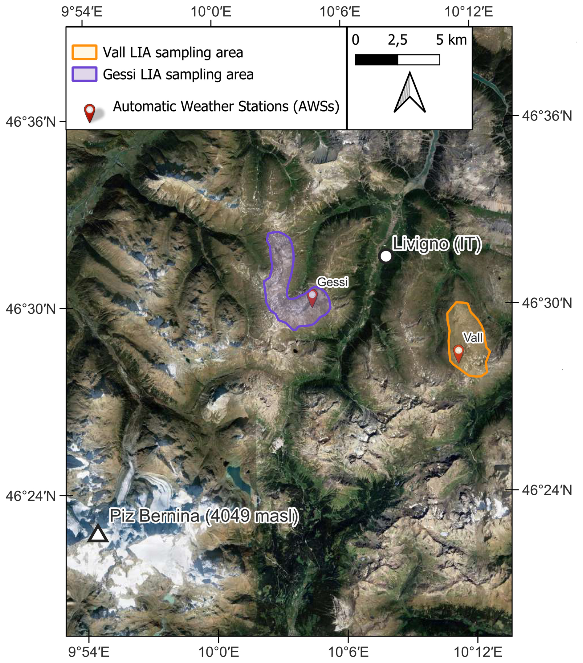
Figure 1 General overview of the model calibration area together with the locations of the two AWSs and the LIA sampling areas.

To analyze the evolution of the SAR signals over the seasons and their dependency on the snowpack properties, we selected two sampling areas inside the model calibration area (hereafter referred to as regression sampling areas) around two AWSs: Gessi (46°31^′23^′′ N, 10°7^′27^′′ E – 2633 m a.s.l.) and Vall (46°28^′37^′′ N, 10°11^′28^′′ E – 2660 m a.s.l.). Both areas were defined with a 25 m square buffer around the locations of the AWSs, which was adjusted to exclude zones affected by wind deposition and erosion, while aiming to keep the morphology as homogeneous as possible. Both regression sampling areas have slopes ranging from 0 to 12°, with the AWSs located on flat terrain, and a predominant northwest slope orientation. The area surrounding the Gessi AWS is a typical periglacial environment, characterized by a landscape of scattered stones interspersed with moss and alpine steppe; the presence of permafrost cannot be excluded. In contrast, the area around the Vall AWS exhibits a smaller concentration of stones and is dominated by alpine steppe, interspersed with smooth bedrock outcrops. To analyze the relationship of SAR signal variations with the LIA, we selected two larger areas around the location of the AWSs (hereafter referred to as LIA sampling areas) to ensure a heterogeneous LIA distribution (see Fig. 1). For these areas, a 2 km buffer was applied around the location of the AWSs, with elevation differences limited to ±200 m. Zones with anthropogenic features, such as ski slopes or zones where snow cover is heavily influenced by ski touring and freeride tracks, were excluded based on the experience of local avalanche forecasters. The LIA sampling areas surrounding the two AWSs display comparable yet heterogeneous land-cover compositions, characterized by alternating zones of alpine steppe, talus deposits, occasional bedrock outcrops, and dispersed large boulders. It is important to note that the regression sampling areas were included within the LIA sampling areas, but the former represented only a small fraction of the latter. Therefore, despite the partial overlap, the results obtained from analyzing the second area were largely independent from those related to the first, as they were mainly driven by new additional data.

To validate the results, we selected a 50 km × 50 km area inside the Norwegian model validation area where in situ measurements were available. Within this area, we applied a 25 m square buffer around each measurement location to sample the model estimations (hereafter referred to as Norwegian validation sampling areas). Concerning the Swiss validation area, we considered an area of approximately 2 km² where a photogrammetric snow depth product was available (as will be shown later in the paper, our analysis predominantly focused on snow depth retrieval). Images of the two validation areas will be presented in Sect. 4.3 together with the related results.

2.2 SAR data

In the present study, we employed freely available level-1 GRD data products from the Sentinel-1 platform, which provides data from a dual-polarization C-band Synthetic Aperture Radar (SAR) instrument at 5.405 GHz. The data were acquired in Interferometric Wide swath mode (IW), with an original resolution of 5 m in range and 20 m in azimuth. Both VV and VH polarization are available and the platform is right-looking. During the SAR data preprocessing phase, as well as to compute the local incidence angle for the two AGs, we used the freely-available Copernicus GLO-30 DEM (digital elevation model) with a 30 m cell resolution (European Union, 2021).

For the calibration of our model we selected two acquisition geometries (AGs) that entirely cover the calibration area, taking advantage of the different acquisition times and look directions. The first AG, with relative orbit number 168, was in the descending direction and was acquired around 05:00 UTC. The second orbit, with relative orbit number 15, was in the ascending direction and acquired around 17:00 UTC. The different acquisition times provided valuable information for monitoring snowpack conditions, which could vary significantly between morning and afternoon at this latitude. In the present study, we focused on the period from October 2022 to July 2024, covering two full snow seasons. Given the Sentinel-1 revisit time of 12 d, a total number of 57 descending plus 59 ascending Ground Range Detected (GRD) products were downloaded in Cloud Optimized Geotiff format (COG) (Copernicus, 2025).

For the validation of the model we downloaded Sentinel-1 GRD products over the Norwegian validation area for the months of December 2024 and January 2025. The two AGs had relative orbit numbers 131, with descending direction and acquisition time around 05:00 UTC, and 95, with ascending direction and acquisition time around 17:00 UTC. Concerning the Swiss validation area, we downloaded a Sentinel-1 GRD product acquired on 9 January 2022 at 17:00 UTC (AG 15).

2.3 Weather and snowpack measurements

Concerning the calibration area, the weather data utilized to run the snowpack evolution model were collected by the two AWSs, which operated throughout the analysis period. These measurements included air and snow-surface temperature, snowpack height, relative humidity, atmospheric pressure, wind speed and direction, and incoming shortwave radiation. It should be noted that these AWSs are routinely employed for snowpack simulations to support avalanche forecasting within the Livigno municipality (additionally, standard in situ snow stratigraphies are routinely performed in the backcountry areas to calibrate model parameters and validate simulation outputs; Monti et al., 2016). During the 2022–2023 winter season, meteorological conditions were marked by below-average precipitation. The maximum HS recorded at the Vall station was 146 cm on 22 April 2023. Field observations revealed that the combination of low temperatures and reduced snowpack thickness led to significant constructive metamorphism, resulting in a generally low-density snowpack dominated by depth hoar and faceted grains in the deeper layers (McClung and Schaerer, 2023). In contrast, the 2023–2024 winter season experienced frequent Atlantic weather systems, leading to above-average temperatures and precipitation. The maximum HS during this period was 322 cm, recorded at the Vall station on 3 April 2024. These conditions produced a dense and warm snowpack overall.

To the Norwegian validation area are associated 27 in situ snow stratigraphies or snow depth manual observations, already presented by Engeset et al. (2018). These measurements were acquired between 10 December 2024 and 15 January 2025 in dry snow conditions. On the other hand, to the Swiss validation area is associated a snow depth raster obtained by differentiating a summer digital surface model (DSM) realized with a UAV–photogrammetric survey with another DSM carried out on 12 January 2022 in dry snow condition (Bühler et al., 2022). The dataset has an original resolution of 10 cm. These measurements were made 3 d after the corresponding SAR acquisitions, but the snowpack did not change significantly during that period, so the temporal offset is not expected to strongly affect the comparison.

3 Methods

3.1 Snowpack modelling

Snow observations directly measured by the AWSs were integrated with data derived by snowpack simulations. For this purpose, the SNOWPACK software was used (Bartelt and Lehning, 2002), with the operational setting employed for avalanche forecasting purpose in Livigno. The simulations were performed for a flat terrain (no preferential exposition), where the model was forced to follow the snowpack height measured by the AWSs, thus also simulating wind-driven snow erosion. The simulated data had an hourly temporal resolution. For each date and time of the available SAR acquisitions, we extracted the following snowpack variables (Xsv):

• snow height directly measured by the AWSs (HS);

• snow surface temperature directly measured by the AWSs (T_ss);

• simulated snow water equivalent (SWE);

• average simulated snow density of the entire snowpack (ρ_s);

• average simulated grain size, referring to the grain diameter, of the entire snowpack (E_s);

• average simulated liquid water content of the entire snowpack (LWC) expressed in percent by volume;

• height of the new snow of the last 24 h (HN24).

3.2 SAR data processing

We used the open-source software SNAP for the entire standard preprocessing workflow of the Sentinel-1 GRD products, as well as for extracting the LIA. Initially, we applied the orbit state vectors provided by the satellite facility and then we performed radiometric calibration following the beta-nought (β⁰) convention. Next, we removed the radiometric variability associated with topography using the Radiometric Terrain Correction algorithm proposed by Small (2011), obtaining the backscatter coefficient gamma-nought (γ⁰). This coefficient was subsequently subjected to geometric terrain correction and speckle filtering using the Lee filter with a 9×9 pixels window size and 2 looks (Yommy et al., 2015). The original resolution of the GRD products was 10 m.

For each preprocessed scene we computed the simplified DpRVI_c index as proposed by Feng et al. (2024):

$$\begin{array}{}\text{(1)}& {\mathrm{DpRVI}}_{\mathrm{c}}={\displaystyle \frac{({\mathit{\gamma }}_{\mathrm{VH}}^{\mathrm{0}}{)}^{\mathrm{2}}+\mathrm{3}{\mathit{\gamma }}_{\mathrm{VH}}^{\mathrm{0}}{\mathit{\gamma }}_{\mathrm{VV}}^{\mathrm{0}}}{({\mathit{\gamma }}_{\mathrm{VH}}^{\mathrm{0}}+{\mathit{\gamma }}_{\mathrm{VV}}^{\mathrm{0}}{)}^{\mathrm{2}}}},\end{array}$$

where ${\mathit{\gamma }}_{\mathrm{VH}}^{\mathrm{0}}$ represents the backscatter coefficient γ⁰ in cross-polarization, while ${\mathit{\gamma }}_{\mathrm{VV}}^{\mathrm{0}}$ represents the backscatter coefficient γ⁰ in co-polarization. Both of them are measured in linear scale. Note that for a fixed value of ${\mathit{\gamma }}_{\mathrm{VH}}^{\mathrm{0}}$, the DpRVI_c index decreases as ${\mathit{\gamma }}_{\mathrm{VV}}^{\mathrm{0}}$ increases because ${\partial }_{{\mathit{\gamma }}_{\mathrm{VV}}^{\mathrm{0}}}{\mathrm{DpRVI}}_{\mathrm{c}}={\mathit{\gamma }}_{\mathrm{VH}}^{\mathrm{0}}({\mathit{\gamma }}_{\mathrm{VH}}^{\mathrm{0}}-\mathrm{3}{\mathit{\gamma }}_{\mathrm{VV}}^{\mathrm{0}})/({\mathit{\gamma }}_{\mathrm{VH}}^{\mathrm{0}}+{\mathit{\gamma }}_{\mathrm{VV}}^{\mathrm{0}}{)}^{\mathrm{3}}<\mathrm{0}$ since in general ${\mathit{\gamma }}_{\mathrm{VH}}^{\mathrm{0}}\le {\mathit{\gamma }}_{\mathrm{VV}}^{\mathrm{0}}$ (Mandal et al., 2020; see also Fig. 3). On the other hand, for a fixed value of ${\mathit{\gamma }}_{\mathrm{VV}}^{\mathrm{0}}$, the DpRVI_c index increases as ${\mathit{\gamma }}_{\mathrm{VH}}^{\mathrm{0}}$ increases. Using data from the AWSs and Sentinel-2 optical imagery, we selected and averaged snow-free summer images to obtain a summer reference image (${\mathrm{DpRVI}}_{\mathrm{c}}^{\mathrm{sr}}$) for each of the two AGs. We then computed a new (adimensional) snow index, named Snow Index SAR (SIsar), as follows:

$$\begin{array}{}\text{(2)}& \text{SIsar}={\mathrm{DpRVI}}_{\mathrm{c}}\left(t\right)-{\mathrm{DpRVI}}_{\mathrm{c}}^{\mathrm{sr}},\end{array}$$

where t represents the acquisition time over the snow season.

To analyze the relationship between the SIsar index and each of the Xsvs, we extracted SIsar–time-series for the two regression sampling areas and the two satellite orbits. Wet snow presence in each scene was identified using γ⁰ images, following the algorithm proposed by Nagler et al. (2016), and dates with wet snow conditions were neglected from the study. The Nagler's method was performed using reference images from the same acquisition dates as those used for ${\mathrm{DpRVI}}_{\mathrm{c}}^{\mathrm{sr}}$ computation. The SIsar values in the time series were computed by averaging the values within the 50 m × 50 m regression sampling areas for the two different AGs (similarly to Pettinato et al. (2013), we noticed that this was the optimal choice to balance spatial resolution and temporal signal stability). The pixels with negative SIsar values along the snow season were excluded and we hypothesized that this anomalous effect was related to the LIA. For analyzing the dependence between our index and the LIA, we grouped and averaged the SIsar values for LIA classes of 5 and 2° within the two LIA sampling areas (in this case, we considered the values of each 10 m × 10 m pixel separately and no averaging was performed since each pixel was characterized by a different LIA). This last analysis was conducted under snow-free conditions as well as on several dates during the snow season. In this case, the pixels with negative SIsar values were not excluded in order to verify our previous hypothesis. The SIsar values related to each 50 m × 50 m Norwegian validation sampling areas were again computed by averaging the values of each pixel. The Swiss validation area was treated in a similar manner: we computed SIsar values over the SAR scene at 50 m spatial resolution and applied a 3×3 pixel median filter to reduce outliers and to handle for a few missing values in the photogrammetric raster. Subsequently, the photogrammetric snow depth raster was resampled to the same resolution using bilinear interpolation. The presence of dry snow was verified with the Nagler's method in all validation areas, moreover for the validation we did not remove the pixels with negative SIsar values (the reason of this different choice will be clear in Sect. 4.2).

3.3 Mathematical modelling

Based on the theoretical background, the SIsar index was assumed to be a function of the snowpack properties. Therefore, it could be expressed as:

$$\begin{array}{}\text{(3)}& \text{SIsar}=\text{SIsar}(\text{HS},{\mathit{\rho }}_{\mathrm{s}},T_{\mathrm{ss}},E_{\mathrm{s}},\text{LWC},\text{HN24}\mathrm{\dots }).\end{array}$$

Our objective was to identify the most important snowpack variable Xsv, to approximate the SIsar index as

$$\begin{array}{}\text{(4)}& \text{SIsar}\simeq f\left(\text{Xsv}\right),\end{array}$$

where f was a suitable unknown function to be derived. Moreover, we then studied the dependence of the SIsar index on the LIA in order to refine Eq. (4), namely we would like to write:

$$\begin{array}{}\text{(5)}& \text{SIsar}\simeq \stackrel{\mathrm{̃}}{f}(\text{Xsv},\text{LIA}),\end{array}$$

where, again, $\stackrel{\mathrm{̃}}{f}$ had to be derived. Finally, since the LIA is always known, by inverting Eq. (5) we would be able to compute an approximation Xsv_mdl (“mdl” stands for modelled) for the variable Xsv.

To this end, we initially implemented a random forest algorithm to assess the importance of the snowpack variables in predicting the values of the SIsar index sampled within the two regression sampling areas. The random forest was performed using the R programming environment, running the algorithm proposed by Breiman (2001). This approach allows for the estimation of the importance of independent variables in predicting the dependent variable. Variable importance is assessed using the permutation method, which involves randomizing the values of each variable one at a time and evaluating the resulting decrease in model performances. It is worth noticing that the SWE variable was excluded from the random forest model as it is dependent on other variables, indeed $\text{SWE}=\text{HS}\cdot ({\mathit{\rho }}_{\mathrm{s}}/{\mathit{\rho }}_{\mathrm{w}})$, where ρ_w denotes the water density. The purpose of this analysis was purely qualitative, and the results were then validated through a statistical analysis. This latter analysis was conducted for the individual time series derived from the two regression sampling areas and the two separate AGs, as well as for all the data treated together. Specifically, Spearman's correlation coefficient (SCC) and Pearson's correlation coefficient (PCC) were calculated, and their significance was verified through the associated p value obtained from a Z test and a t test, respectively. The SCC was used to assess the presence and the nature (positive or negative) of the correlation between the SIsar index and the target Xsv. The SCC is a non-parametric measure, meaning it does not assume any specific distribution of the data, and it helps to identify monotonic relationships, whether linear or non-linear. In contrast, the PCC was used to determine whether the relationship between the SIsar index and the chosen Xsv was linear or not. The PCC measures the strength and direction of a linear relationship between the data, and the assumption that those data are normally distributed must be made to verify the significance of the test (Hauke and Kossowski, 2011). For the variables that showed a significant linear correlation, we then fitted a linear regression model.

At this stage of the analysis, we selected the Xsv which showed the best linear correlation with the SIsar index, and for which we could assume the theoretical property that SIsar≃0 corresponds to snow-free conditions. Thus, we expressed the following relation:

$$\begin{array}{}\text{(6)}& \text{SIsar}\simeq f\left(\text{Xsv}\right)=a\cdot \text{Xsv},\end{array}$$

where a>0 was derived with the least squares method. Therefore, the initial (linear) model for Xsv was given by

$$\begin{array}{}\text{(7)}& {\mathrm{Xsv}}_{\mathrm{mdl}\mathrm{\_}\mathrm{lin}}={\displaystyle \frac{\text{SIsar}}{a}},\end{array}$$

where Xsv_{mdl_lin} denotes the linear model-based approximation of Xsv. Concerning the study of the dependence of the SIsar index on the LIA, we expressed this relationship as:

$$\begin{array}{}\text{(8)}& \text{SIsar}\simeq \stackrel{\mathrm{̃}}{f}(\text{Xsv},\text{LIA})=g\left(\text{LIA}\right)\cdot \text{Xsv},\end{array}$$

where the function g was derived again with the least squares method and its shape was chosen according to the distribution of the data derived from the LIA sampling areas. Indeed, when selecting a time and a LIA sampling area, we could assume (especially at the beginning of the winter season, when wind redistribution and variations in melting or metamorphism are not very influential) that the snowpack variable Xsv remained constant in that zone. On the other hand, the LIA took on many different values. For this reason, the function g could be approximated as $g\left(\text{LIA}\right)\simeq \text{SIsar}/\text{Xsv}$, which should be independent on Xsv. Therefore, the final model for estimating Xsv was:

$$\begin{array}{}\text{(9)}& {\mathrm{Xsv}}_{\mathrm{mdl}\mathrm{\_}\mathrm{LIA}}={\displaystyle \frac{\text{SIsar}}{g\left(\text{LIA}\right)}},\end{array}$$

where Xsv_{mdl_LIA} denotes the approximation of Xsv depending on the local incidence angle.

3.4 Model validation strategy

The validation of our model for approximating Xsv was divided into four parts. Initially, we compared, in terms of root mean squared error (RMSE) and mean absolute error (MAE), the approximations for Xsv given by Eqs. (7) and (9), using as reference the measurements of the two AWSs (Xsv_msr; “msr” stands for measured) inside the model calibration area. Secondly, we performed a mathematical analysis to establish the validity of the LIA dependency through the function g. When we initially derived the value a we considered values of the SIsar index related to different LIAs. For this reason, the weighted average value $\stackrel{\mathrm{‾}}{g}$ of the function g should be similar to a. Note that we had to consider a weighted average because some LIAs were more recurring than others. Recall that the regression sampling areas and the LIA sampling areas were effectively independent of each other. Thirdly, using Eq. (9), we computed the values of Xsv_{mdl_LIA} for the Norwegian validation sampling areas and, to demonstrate the model's applicability in a location significantly different from the one it was calibrated on, we compared those values with the field measurements. Finally, using again Eq. (9), we computed the values of Xsv_{mdl_LIA} for the Swiss validation area and we compared them to the photogrammetric data in order to validate the model with a large dataset.

4 Results

4.1 SIsar index and snowpack variables

Due to the limited dataset available, the results of the random forest analysis are exploratory. The importance values of the variables are uniformly low and, therefore, not reported, as they are likely affected by the small sample size and should not be overinterpreted. Nevertheless, the random forest model suggests that the variable HN24 is not important for predicting the SIsar index, while HS emerged as the most important predictor, followed by ρ_s, E_s, LWC, and T_ss. The results of the statistical analysis, conducted on the entire dataset (which includes all regression sampling areas and acquisition geometries), are presented in Table 1. The analysis reveals significant correlations between the SIsar index and several variables, including HS, SWE, ρ_s, and E_s. Specifically, there is a moderate-to-strong positive relationship with both HS and SWE, a moderate positive correlation with ρ_s, and a moderate-to-low negative correlation with E_s. These findings align with the results from the random forest model. The PCCs and the related p value tests indicate that the linear relationships between the SIsar index and both HS and SWE are strong, while no robust linear relationship is found between the SIsar index and ρ_s. Moreover, the p values associated to the linear regression model show that, for both HS and SWE, the regression slope is significant. However, only for HS the intercept is not significant. Therefore, only for HS, we can set the intercept to zero, implying that snow-free conditions should correspond to a value of SIsar≃0 (see Sect. 3.3). This, together with the fact that the best PCC corresponds to HS, supports the selection of this variable as the candidate Xsv for the model. Therefore, hereafter we set Xsv=HS. In particular, the quality of the linear regression with intercept set equal to zero is almost the same as the one obtained for a generic intercept, indeed the R² coefficients are 0.493 and 0.495 respectively. The coefficient a of the linear relationship between HS and the SIsar index (see Eq. 6) is approximately $\mathrm{6.00}\times {\mathrm{10}}^{-\mathrm{4}}{\mathrm{cm}}^{-\mathrm{1}}$, as reported in Fig. 5a.

Table 1 Summary of the results of the statistical analysis for each snowpack variable Xsv. The linear regression is performed only for those variables showing a significant and large PCC.

The results of the statistical analysis conducted for each individual regression sampling area are not presented in tabular form for brevity. However, the findings are consistent with those reported for the analysis conducted on the entire dataset. Focusing only on the most influential variables, a strong positive PCC with the SIsar index is observed for HS and SWE across all areas and AGs. In particular, the highest PCC values for HS and SWE are at Vall for AG 15, with PCC equal to 0.802 and 0.800, respectively. Additionally, the correlation intensity order among the variables is in line with the results from the analysis of the entire dataset, except for the Gessi area in AG 168, where SWE shows a slightly better linear correlation with the SIsar index than HS (PCC equal to 0.761 against 0.756). Finally, the best correlations are in general related to the AG 15 (afternoon).

4.2 SIsar index and local incidence angle

Figure 2 shows examples of the behavior of the SIsar index for 5° LIA classes across the different LIA sampling areas, at different times during the snow season, and under snow-free conditions. In both areas, for all acquisitions with snow-free conditions, the SIsar index on average remains approximately constant as the LIA increases, with values close to zero. When analyzing the relationship in both LIA sampling areas for all dates with snow cover, we first observe that the SIsar index shows negative values for angles approximately smaller than 30°, even if HS is not zero. For all these acquisitions, for angles greater than approximately 30°, the relationship between the SIsar index and the LIA follows a parabolic shape, which suggests a relationship between them in the presence of snow.

Figure 2 Box plots of 5° LIA classes vs. SIsar index values over the course of the snow accumulation season (i.e., for increasing values of HS measured by the AWSs within the LIA sampling areas). (a) Gessi AG 15, 8 August 2023, snow-free conditions. (b) Gessi AG 168, 23 November 2023, HS_msr=60 cm. (c) Gessi AG 15, 24 November 2023, HS_msr=60 cm. (d) Vall AG 168, 29 December 2023, HS_msr=100 cm.

As one can notice from Fig. 3, the point where the curves showing the relation between the LIA and the SIsar index intersect the x axis is consistently around 25–30°, and again we see that the relationship between the SIsar index and the LIA follows a parabolic shape for larger angles. In particular, as HS increases the parabolic shape expands vertically upwards. This suggests that the SIsar index can be expressed as Eq. (8). Figure 3 also reports the behaviors of the DpRVI_c index and of the single backscatter components ${\mathit{\gamma }}_{\mathrm{VH}}^{\mathrm{0}}$ and ${\mathit{\gamma }}_{\mathrm{VV}}^{\mathrm{0}}$ as the LIA varies. Under snow conditions, the DpRVI_c index attains values smaller than under snow-free conditions only for LIAs smaller than 25–30°, in line with the SIsar index behavior. Unlike the latter, its values related to the summer acquisition depend on the LIA. Note that ${\mathit{\gamma }}_{\mathrm{VV}}^{\mathrm{0}}$ increases with HS for LIAs below approximately 20°, in line with the findings of Jans et al. (2025), while it appears to be independent on HS for larger LIAs. However, it decreases as the LIA varies between 20 and 80°. On the other hand, ${\mathit{\gamma }}_{\mathrm{VH}}^{\mathrm{0}}$ shows a more complex behavior as the LIA varies. Interestingly, for LIA values below 30°, it reaches smaller values under snow-covered conditions than under snow-free conditions. However, we observe the opposite trend for larger LIAs and a positive correlation with HS in line with the results of Brangers et al. (2024).

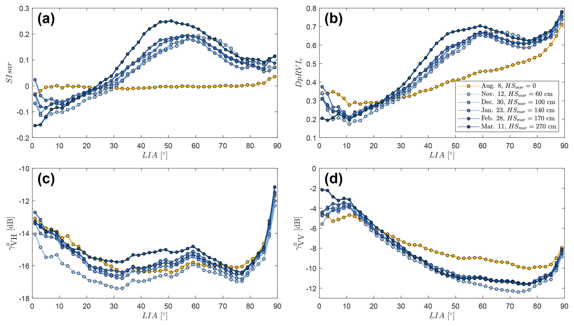
Figure 3 Mean SIsar (a), DpRVI_c (b), ${\mathit{\gamma }}_{\mathrm{VH}}^{\mathrm{0}}$ (c), and ${\mathit{\gamma }}_{\mathrm{VV}}^{\mathrm{0}}$ (d) values, sampled from the LIA sampling areas, grouped into LIA classes of 2° width. The blue color scale represents the increasing HS values measured by the two AWSs for different acquisition dates along the 2023-2024 season. Yellow points represent the values from an acquisition date in summer 2023. The legend in (b) is the same for all subfigures.

From the least squares method, we obtain the following equation for g(LIA) describing a parabola, as represented in Fig. 4:

$$\begin{array}{}\text{(10)}& g\left(\text{LIA}\right)=a_{\mathrm{0}}+a_{\mathrm{1}}\cdot \text{LIA}+a_{\mathrm{2}}\cdot {\text{LIA}}^{\mathrm{2}},\end{array}$$

where the LIA is expressed in degrees, $a_{\mathrm{0}}=\mathrm{4.41}\times {\mathrm{10}}^{-\mathrm{3}}{\mathrm{cm}}^{-\mathrm{1}}$, $a_{\mathrm{1}}=\mathrm{2.04}\times {\mathrm{10}}^{-\mathrm{4}}$ per degree cm⁻¹, and $a_{\mathrm{2}}=-\mathrm{1.80}\times {\mathrm{10}}^{-\mathrm{6}}$ per degree cm⁻¹. The resulting R² coefficient is equal to 0.695. The zeros of g(LIA) are approximately 29.1 and 84.4°. Since we observe that for LIA values below approximately 30° the SIsar index is always negative, even when HS is nonzero, we exclude all areas with LIA<30° in the implementation of the final model (this confirms our initial hypothesis that those negative SIsar values are related to the LIA; see Sect. 3.2). Areas with LIA>80° are also removed because they are in shadow. Note that, due to these choices, Eq. (9) is well-defined since g(LIA)≠0 for all LIAs of interest.

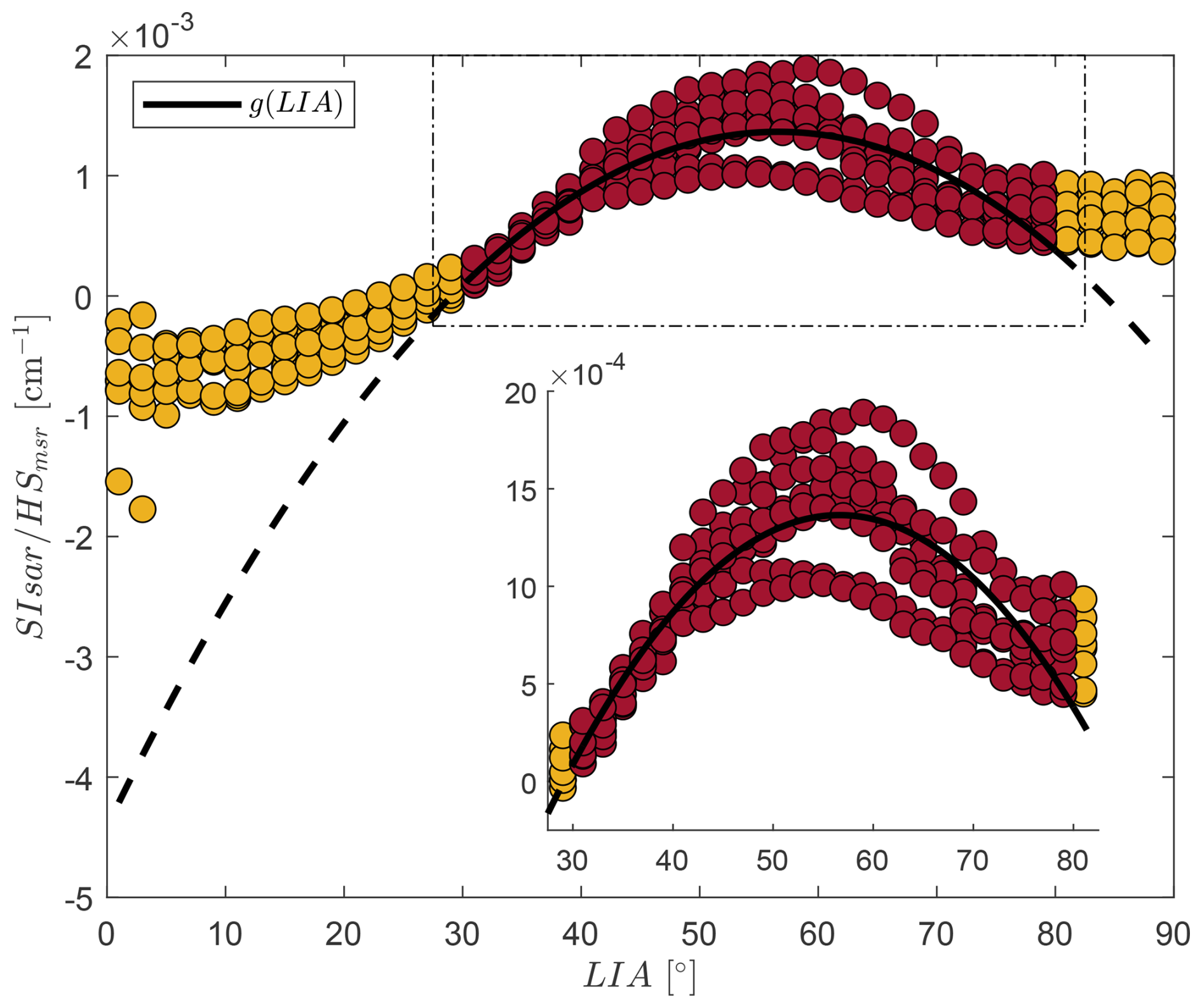
Figure 4 Mean SIsar values normalized by HS measured by the AWSs grouped into LIA classes of 2° width. Data derive from the beginning of the season, when we could assume that HS was representative of the entire LIA sampling areas. Values for LIA<30° and LIA>80° are reported in yellow, while values between 30 and 80° in red. In black we report the function g(LIA), inferred on the red data.

4.3 Models comparison and validation

When applied to the calibration area, the model for HS given by Eq. (7) leads to a RMSE equal to 57.2 cm and a MAE equal to 46.0 cm. With the LIA correction, the errors drop significantly, indeed using Eq. (9) the RMSE becomes 34.6 cm while MAE 28.3 cm. These values represent a 39.5 % decrease in RMSE and a 38.5 % decrease in MAE. Plotting HS_{mdl_LIA} against HS_msr (Fig. 5b), we observe that ${\mathrm{HS}}_{\mathrm{mdl}\mathrm{\_}\mathrm{LIA}}\simeq c_{\mathrm{1}}\cdot {\mathrm{HS}}_{\mathrm{msr}}$, with c₁=0.841. It is important to note that a perfect model would lead to a value of c₁ equal to 1. To mathematically verify the validity of g(LIA) we compute its weighted average $\stackrel{\mathrm{‾}}{g}$ as explained in Sect. 3.4, obtaining $\stackrel{\mathrm{‾}}{g}=\mathrm{9.70}\times {\mathrm{10}}^{-\mathrm{4}}{\mathrm{cm}}^{-\mathrm{1}}$, which is of the same order of magnitude as the coefficient $a=\mathrm{6.00}\times {\mathrm{10}}^{-\mathrm{4}}{\mathrm{cm}}^{-\mathrm{1}}$ of Eq. (7). Moreover, using Eq. (9) to estimate HS in the validation area around Tromsø (the Norwegian validation dataset; see Fig. 6b) we obtain an RMSE of 30.7 cm and a MAE of 24.3 cm. Finally, using Eq. (9) to estimate HS in the validation area around Davos (the Swiss validation dataset; see Fig. 7) we obtain an RMSE of 22.4 cm and a MAE of 18.1 cm. See Table 2 for a comparison of the errors and the number of data points.

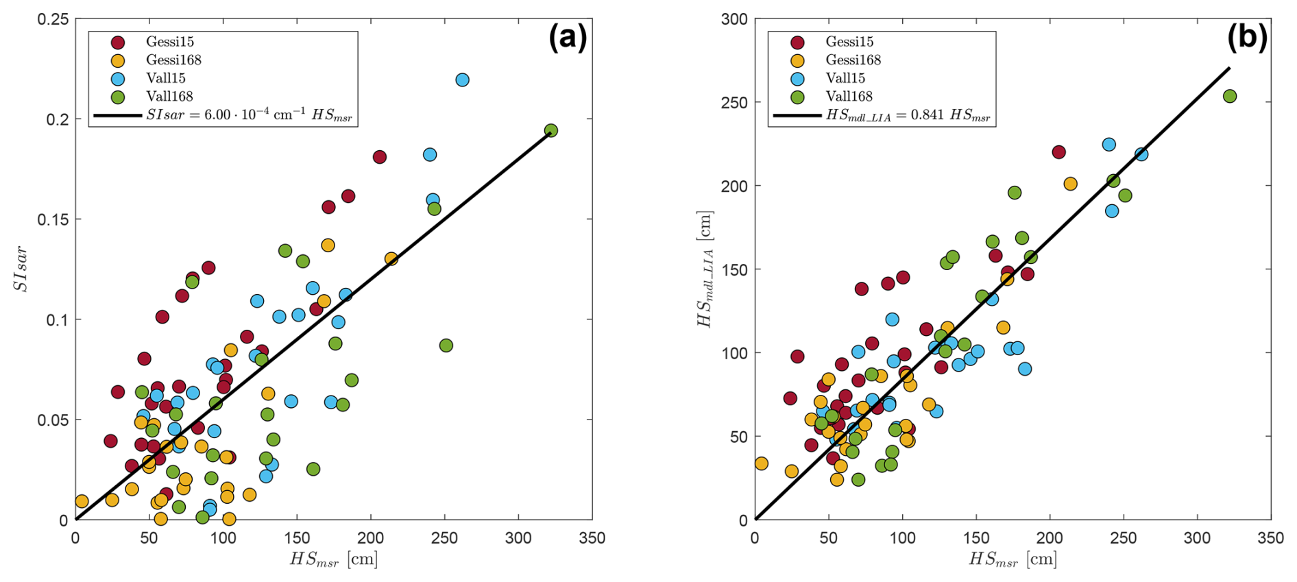
Figure 5 (a) Scatter plot of HS_msr vs. SIsar. (b) Scatter plot of HS_msr vs. HS_{mdl_LIA}. The linear regressions computed with the least square method are also represented.

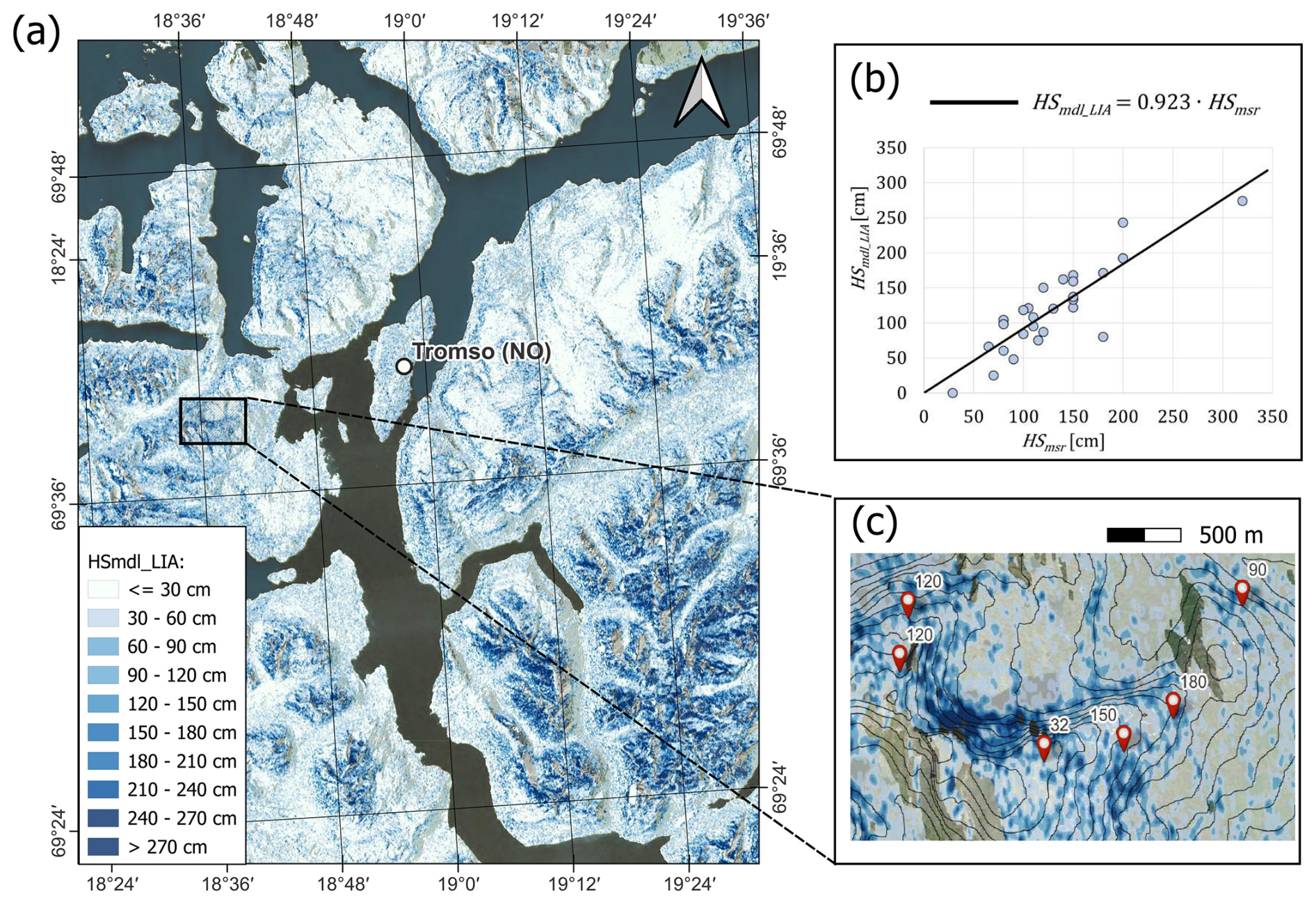
Figure 6 Snow depth estimation for the Norwegian validation area. (a) Overview of HS_{mdl_LIA} between 31 December 2024 and 1 January 2025. (b) HS_msr vs. HS_{mdl_LIA} related to the 27 in situ snowpack observations. (c) Particular of (a) showing in situ observations carried out between 30 December 2024 and 2 January 2025 (no significant variation of HS occurred in this time window).

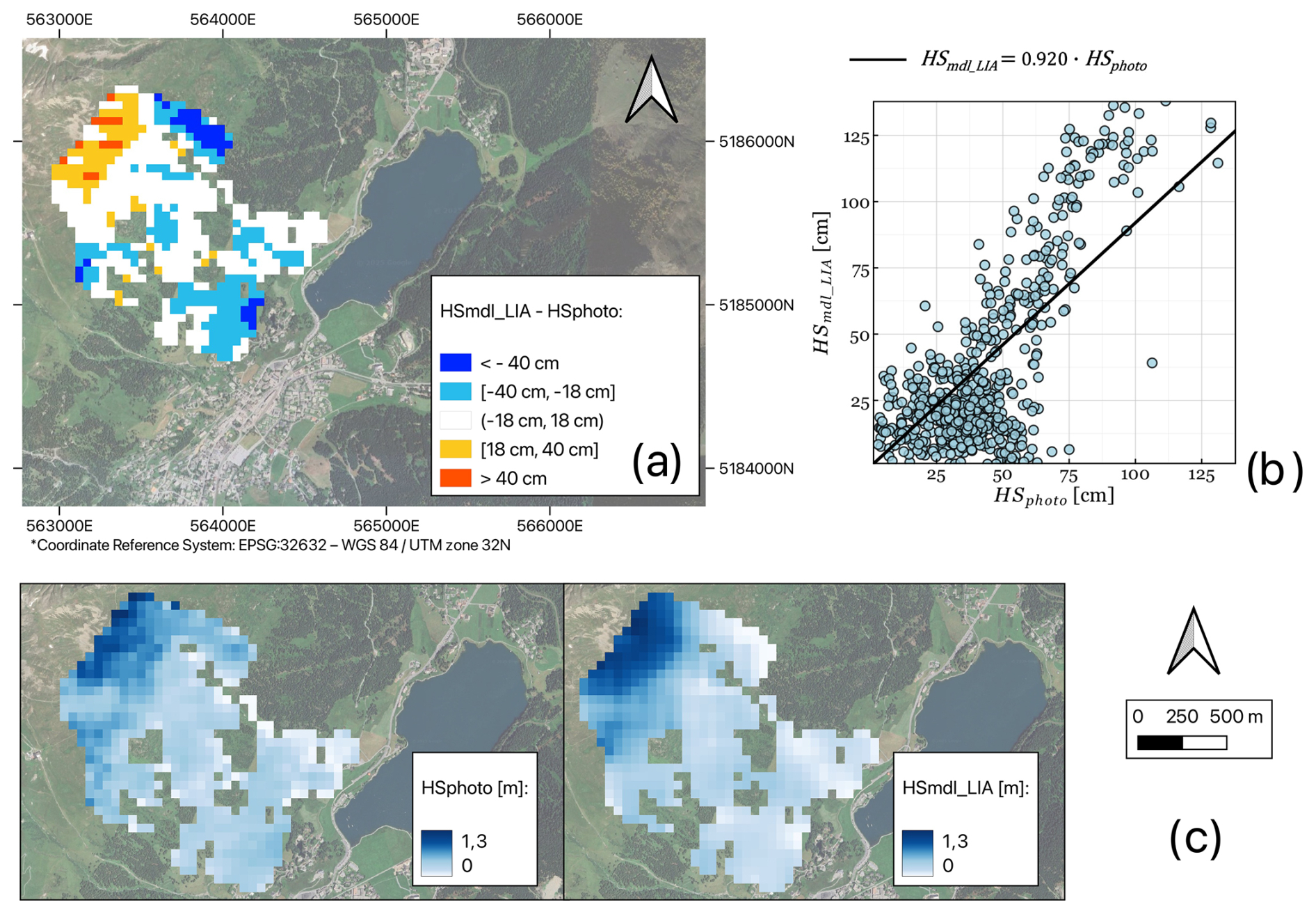
Figure 7 Swiss validation area. (a) Difference between HS_{mdl_LIA} and HS_photo, derived from the photogrammetric survey; the cell size is 50 m. (b) HS_{mdl_LIA} vs. HS_photo. (c) HS_photo (left) and HS_{mdl_LIA} (right).

Table 2 Errors and number of data points related to the different models and datasets.

5 Discussion

5.1 Correlations of the SIsar index with snowpack variables

The statistical analysis indicates that the SIsar index is a complex function of several snowpack parameters. Nevertheless, since SAR measurements are of great interest, especially in poorly monitored areas where no additional observations are generally available, we aimed to limit the dependency to just one of the most significantly linearly correlated variables. These are HS and SWE, in accordance with several other studies (Snehmani et al., 2015; Lievens et al., 2019; Patil et al., 2020). The selection of HS as candidate Xsv is supported by the fact that it is the only snowpack variable for which the intercept value is not statistically significant, thereby fulfilling the theoretical condition that SIsar≃0 corresponds (on average) to a snow-free state.

The Spearman's correlation coefficient suggests that the SIsar index increases also with ρ_s. One possible explanation for this increase is that thicker and denser snowpacks contain larger snow mass and more grains per unit volume of snow, consequently, there will be more opportunities for signal depolarization, as reported in Lievens et al. (2019). In addition, Tiuri et al. (1984) demonstrated that both the real and imaginary parts of the dry-snow dielectric constant increase with snow density. As this happens, the surface backscatter enhances, while the influence of the underlying soil may be slightly reduced due to the stronger absorption. However, the Pearson's correlation coefficient suggests that the relation between the SIsar index and ρ_s is not linear. This is in line with the linear relationship resulted between the SIsar index and the SWE: if both ρ_s and HS would be linearly correlated with the index, then the SWE would be quadratically correlated with it (this directly follows from the definition of SWE; see Sect. 3.3). Concerning the fact that the intercept can be set equal to zero for HS but not for the SWE, this is probably a consequence of the fact that the SWE is not well-defined in absence of snow: as snow fades away, both its mass and volume tend to zero, implying that ρ_s cannot be defined in absence of snow. A backscatter increase with ρ_s is also observed in Besic et al. (2012), who however demonstrate how the ρ_s influence on SAR-based SWE retrieval is negligible.

Paloscia et al. (2017) observed that the co-polarized band of Cosmo-SkyMed ${\mathit{\sigma }}_{\mathrm{HH}}^{\mathrm{0}}$ increases with larger E_s. Assuming that ${\mathit{\gamma }}_{\mathrm{VV}}^{\mathrm{0}}$ behaves similarly to ${\mathit{\sigma }}_{\mathrm{HH}}^{\mathrm{0}}$, this could explain the slight decrease in the SIsar index that we observe for increasing E_s. Nevertheless, further analysis are required to understand the influence of this parameter. Interestingly, the results do not show a significant correlation between the SIsar index and T_ss even if Baumgartner et al. (1999) demonstrated that SAR backscatter is sensitive to variations in near-surface snow temperature.

Finally, it should be emphasized that the LWC exhibits one of the weakest correlations with the SIsar index, despite its primary role in the snow backscattering mechanism (Tiuri et al., 1984; Nagler and Rott, 2000; Besic et al., 2012). However, this is not surprising since we excluded all acquisitions containing wet snow according to the Nagler's method, which obviously significantly reduced the variability of the LWC.

The statistical analysis conducted for individual regression sampling areas and individual acquisition geometry confirm the one conducted on the entire dataset. The evidence that the Pearson's correlation coefficients for individual stations and acquisition geometry slightly differ from the one obtained when considering all data together suggests that variations in morphology, land cover, and local climatic conditions lead to slight differences in the relationship between the SIsar index and any Xsv. Consequently, a local fitting approach should perform slightly better than a global one. These results are consistent with the findings of Jans et al. (2025).

5.2 Influence of the local incidence angle on the SIsar index

The analysis of the relationship between the DpRVI_c index and the SIsar index with the LIA under snow-free and snow-covered conditions reported in Fig. 3 is revealing. In particular, the findings regarding the two single backscatter components ${\mathit{\gamma }}_{\mathrm{VH}}^{\mathrm{0}}$ and ${\mathit{\gamma }}_{\mathrm{VV}}^{\mathrm{0}}$ are in line with the results presented by Brangers et al. (2024) and Jans et al. (2025), respectively. The increase of ${\mathit{\gamma }}_{\mathrm{VH}}^{\mathrm{0}}$ as HS increases can be explained by the larger volume of snow traversed by the SAR signal, which leads to more opportunities for signal depolarization and by the different interactions with layered structures. The fact that ${\mathit{\gamma }}_{\mathrm{VV}}^{\mathrm{0}}$ shows no dependence on HS indicates that it is primarily influenced by soil properties, further confirming the effectiveness of using depolarization ratios to isolate the snow backscatter contributions. Note, however, that the variations of ${\mathit{\gamma }}_{\mathrm{VH}}^{\mathrm{0}}$ with HS is very small, attaining values very close to those observed under snow-free conditions. This may explain why Strozzi et al. (1997) concluded that HS could not be monitored with C-band SAR due to the low sensitivity of the backscatter components to snow accumulation. Interestingly, we observe that in presence of snow the DpRVI_c index attains values significantly larger than those under snow-free conditions for LIAs above 40°, and its variations with HS is substantial. This confirms that the use of polarization ratios or similar indices increases the sensitivity of SAR to HS variations, enabling its monitoring (Lievens et al., 2019; Feng et al., 2024; Jans et al., 2025).

Focusing on the SIsar index, no significant dependence on the LIA is observed for any of the snow-free acquisitions in either analysis area, with values on average around zero. On the other hand, in all acquisitions under snow-cover conditions, we first observe that SIsar values are negative for low incidence angles, specifically for LIA values below approximately 25–30°. For incidence angles greater than 30°, the relationship between our index and the LIA takes on a parabolic shape, increasing up to around 55° before decreasing again. This suggest that DpRVI_c index variations in presence of snow above the ground are significantly influenced by the LIA, and that the latter must be taken into account for dual-polarimetric SAR retrieval of HS (despite the SAR products were radiometrically terrain corrected for the LIA within the preprocessing phase). A complex relationship between SAR-derived vegetation indexes and LIA has been already demonstrated in the presence of vegetation cover above the ground by Kaplan et al. (2021). Since the influence of a vegetation volume on the DpRVI_c can be linked to the one snow over bare soil (Feng et al., 2024), we believe our observations are valid. As shown in Fig. 2, the presence of outliers in the SIsar index values across the LIA classes is notable. However, such variability is common in this type of experiment and can be attributed to various sources of error, including wind redistribution effects, speckle noise, and spatial variability in snowpack or ground properties.

Since the SIsar index is consistently negative during the accumulation season for LIA values smaller than 30°, snow cover monitoring is not possible in this situation. The negative values of the SIsar index at low LIAs can be primarily attributed to the increase of ${\mathit{\gamma }}_{\mathrm{VV}}^{\mathrm{0}}$ with HS (recall Fig. 3d), consistent with previous observations (Jans et al., 2025), which results in snow-covered DpRVI_c index values lower than those under snow-free conditions. The decrease of the SIsar index values for large LIAs is more difficult to interpret. Some possible explanations include a combination of factors such as the dominant specular scattering mechanism, many pixels being in shadows, different interactions with soil and snowpack structures, and travel path of the signal trough the snow being so long that its energy absorption is no longer negligible, even at C-band (Rott et al., 2021). However, further specific studies are needed to confirm or refute these hypotheses.

All these considerations, together with the fact that the parabolic curve describing the dependence of the SIsar index on the LIA extends upwards as the accumulation season progresses (i.e., as HS increases), support the choice of Eq. (8), and hence also the estimation for HS given by Eq. (9). Note that analogous relationships between the DpRVI_c index and HS cannot be established, due to the index's sensitivity to the LIA under snow-free conditions (see Fig. 3b). Finally, the similar behaviors of the SIsar index normalized by the measured HS in both LIA sampling areas at different times of the snow season (see Fig. 4) suggest that g(LIA) is not significantly dependent on local or temporal conditions. Notice that acquisitions refer to two very different seasons in terms of structure and physical properties of the snowpack.

5.3 Effectiveness of considering the local incidence angle within the model

When we approximate HS trough Eq. (9) (i.e., HS_{mdl_LIA}) we obtain a significant improvement with respect to the usage of Eq. (7) (i.e., HS_{mdl_lin}), both in terms of root mean square error and mean absolute error. Furthermore, the values of the weighted average $\stackrel{\mathrm{‾}}{g}$ of the function g(LIA) is of the same order of magnitude of the slope coefficient a of the linear regression. Differences between the values of $\stackrel{\mathrm{‾}}{g}$ and a are attributed to the several sources of errors: we consider only the most influential snowpack variable, variations in soil properties that we do not consider could affect the values of the SIsar index, and the datasets used to derived a and g(LIA) are different and effectively independent of each other (in particular, the former is much smaller than the latter, which naturally results in a smaller variation of LIAs). This also explains why ${\mathrm{HS}}_{\mathrm{mdl}\mathrm{\_}\mathrm{LIA}}\simeq c_{\mathrm{1}}\cdot {\mathrm{HS}}_{\mathrm{msr}}$ with c₁ not exactly equal to 1: the slope c₁ incorporates the errors deriving from the factors just described. However, the results obtained not only confirm the significance of the relationship between the SIsar index and the LIA, but also indicate that correcting the index with a function accounting for its dependence on the LIA leads to a substantial improvement. Therefore, the LIA has a non-negligible influence on SAR signal depolarization when snow is present above the ground.

The results of the validation performed with the in situ measurements carried out in Tromsø, Norway, and Davos, Switzerland, further support the correctness of the modelling. The relation HS_{mdl_LIA}≃HS_msr is successfully verified, and both the RMSE and the MAE are slightly smaller than the corresponding values obtained for Livigno, Italy. This suggests a global applicability of the model, even if a local calibration with in situ observations is recommended, as already discussed in Sect. 5.1. As shown in Fig. 6, mapping HS_{mdl_LIA} for the Norwegian validation area reveals a high degree of heterogeneity in snow cover distribution. At a large-scale, we observe that zones with greater snow accumulation are generally found at higher elevations (see Fig. 6a). Conversely, at a small-scale, we observe that the snow distribution appears highly irregular, with eroded peaks and ridges, while significant deposits are found in bowls and gullies (see Fig. 6c). This latter observation aligns with both field measurements available for the period under analysis and the regional climate, which is characterized by frequent wind transport events. It is important to note that, within the same acquisition, we used field observations that were proximal to one another (minimum spacing of approximately 100 m) but, being the slopes naturally non-homogeneous, they correspond to different LIAs. This implies that, although the obtained MAE was slightly larger than the one obtained in the work of Lievens et al. (2022), where HS was mapped for a 500 m resolution, or in the one of Feng et al. (2024), the proposed model demonstrates a good ability in describing snow depth variations at the small-scale (i.e., within the same slope). This is particularly relevant for avalanche forecasting purposes, since avalanche forecasters are interested in detecting the complex snow cover heterogeneity of the alpine environment, which is influenced by wind transport, avalanches, and the various metamorphic processes occurring at different aspects (Plattner et al., 2004).

The quality of snow depth retrieval at the slope scale is confirmed by the validation in Switzerland, where the HS mapped with our model was compared with measurements derived from a photogrammetric survey. Indeed, the RMSE and the MAE were even smaller than the ones related to the Norwegian validation area. From Fig. 7a, it is evident that the largest overestimations are concentrated in the upper part of the mountain slope, where the steepest gradients occur and the snowpack may have experienced variations (e.g., snow creep) during the 3 d between the Sentinel-1 GRD acquisitions and the UAV–photogrammetric survey. On the other hand, the largest underestimations are found in the lower part of the slope, where the snowpack is very thin.

5.4 Model limitations and future work

A key limitation of our model is that the SIsar index depends not only on the snow height HS but also on other snowpack properties, such as the average snow density ρ_s and average grain size E_s. In mountain regions, these properties can vary considerably since they are strongly influenced by both elevation and aspect. This variability may result in areas where the model performs slightly better and others where its performance is somewhat reduced. Furthermore, the model's sensitivity to specific snow properties can result in biased snow depth estimates for individual scenes, which supports the use of average summer conditions in the change detection algorithm to minimize error propagation.

As reported in Appendix A, we observe an overestimation of HS when wet snow layers are embedded within dry snow layers. This configuration is typical during the early or late stages of the snow season, particularly when dry snowfall accumulates over an existing wet snow surface due to a decrease in frost level during a precipitation event (Colbeck, 1982). This overestimation can be theoretically interpreted as follows: both ${\mathit{\gamma }}_{\mathrm{VV}}^{\mathrm{0}}$ and ${\mathit{\gamma }}_{\mathrm{VH}}^{\mathrm{0}}$ should drop in presence of wet snow since the signal is absorbed and hence unable to penetrate further in depth. However, as observed from analyzing the data, the presence of dry snow on the surface results in a ${\mathit{\gamma }}_{\mathrm{VH}}^{\mathrm{0}}$ increase, which is more sensitive to volumetric backscatter than ${\mathit{\gamma }}_{\mathrm{VV}}^{\mathrm{0}}$. This implies a significant increase of the DpRVI_c index since it increases as the difference between co- and cross- polarization backscatter decreases. Under these conditions, the method of Nagler et al. (2016) used for SAR-based wet snow retrieval may fail since it relies on both VV and VH bands. Notably, in these conditions, the average liquid water content (LWC) of the snowpack is not particularly large, considering that an LWC threshold of 1 % is commonly used to distinguish dry from wet snow (Mitterer et al., 2013).

The variations of HS_{mdl_LIA} in bare-soil conditions reflect the dependence of DpRVI_c by external factors, such as soil moisture, ground surface temperature, and variations in low-lying vegetation (Das and Pandey, 2024). This confirms that the method is inherently unable to clearly discriminate between the presence and absence of snow, as noted in Jans et al. (2025). Indeed, SIsar≃0 in snow-free conditions (see Sect. 3.3) is verified only on average, not for the single acquisition (see Appendix A). Moreover, even if further studies are needed to confirm this behavior, the high number of pixels with negative SIsar values at the beginning of the snow season confirms what reported in Lemos and Riihelä (2025), who demonstrates the difficulties of Sentinel-1 based HS retrieval in very thin snowpacks.

Since the model was calibrated with snowpacks not deeper than 300 cm, its validity for thicker snow accumulations remains untested. Future studies will address these gaps, particularly focusing on DpRVI_c variations in snow-free conditions and explore potential model adjustments for deeper snowpacks, also considering that, theoretically, the signal absorption by Sentinel-1 may become non-negligible for very thick snow layers. Moreover, our study focused on alpine terrain, suggesting that the quality of snowpack height estimations under different terrains and soil covers should be assessed.

When mapping HS over the validation area near Davos (Switzerland), we observed the presence of few patchy outliers. These anomalous pixels likely resulted from the sensitivity of the SIsar index to local variations in snow cover conditions or changes in soil properties between the snow-covered and summer reference acquisitions. However, these outliers could be effectively reduced by applying a median filter over a small pixel window (see Sect. 3.2). We therefore recommend using this filter as a post-processing step.

Finally, it is known that the presence of melt-freeze crusts within the snowpack can strongly affect both co- and cross-polarized backscatter coefficients (Brangers et al., 2024), and thus also the performance of our model.

6 Conclusions

In this study, we presented a novel mathematical model that enhances small-scale snow depth monitoring leveraging dual-polarimetric Sentinel-1 SAR data. Specifically, we introduced a new index, named Snow Index SAR (SIsar), which is defined as the difference between the Dual Polarimetric Radar Vegetation Index (DpRVI_c) computed under snow-covered conditions and average snow-free conditions. The model was calibrated using two independent datasets from the Livigno area (Italy, Central Italian Alps), which include data collected from two proximal automatic weather stations and simulated with the SNOWPACK snow cover model. These datasets span two winter seasons and cover two different acquisition geometries.

A statistical analysis revealed that the SIsar index is influenced by several snowpack variables. In particular, it shows a linear correlation with the snowpack height and the snow water equivalent, while statistically significant relationships were also found with the average snowpack density and grain size. The SIsar index generally increases with these quantities, except for the average grain size, where a low negative correlation was observed. The strongest linear correlation is with the snowpack height, so we initially applied a linear regression model to estimate snow depth from SIsar values. Notably, the model aligns well with theoretical expectations, confirming that SIsar≃0 corresponds (on average) to snow-free conditions.

A key result of this study is the demonstration of the strong influence of the local incidence angle (LIA) on the SIsar index in presence of snow, despite the SAR products are radiometrically terrain corrected for the LIA within the preprocessing phase. For angles below 30°, the SIsar index is almost always negative, a behavior we explained theoretically. Between 30 and 80°, its relationship with the LIA follows a parabolic curve. The derivation of this curve allowed us to correct for the angular dependence of signal depolarization for increasing snowpack height. This correction significantly improved snowpack height estimations compared to the initial linear model, reducing the mean absolute error (MAE) by 38.5 % and the root mean square error (RMSE) by 39.5 %.

The final model was verified and validated using two independent datasets: field observations acquired in Tromsø (Norway) and a photogrammetric snow depth products realized near Davos (Switzerland). The validation results showed a RMSE of 30.7 cm and a MAE of 24.3 cm in Tromsø, and a RMSE of 22.4 cm and a MAE of 18.1 cm in Davos, providing preliminary evidence of the model's potential for global applicability. In addition to the dependence of our index on several snowpack properties, a supplementary analysis identified the summer DpRVI_c index variations and the presence of wet snow layers inside the snowpack as significant sources of error.

Appendix A: Wet snow and summer SIsar index-variations

To further investigate the results, we compared the modelled snowpack height (i.e., HS_{mdl_LIA}) with the SNOWPACK simulated stratigraphies on the two regression sampling areas and across two seasons (2022/23 and 2023/24). We observed that the average liquid water content (LWC) was nonzero, albeit very low, on certain days when Nagler's method did not indicate the presence of wet snow. Looking at the stratigraphies, we noticed that in these dates there were wet snow layers embedded within dry snow layers. As illustrated in Fig. A1 for Gessi with AG 15, overall, the HS_{mdl_LIA} exhibits larger fluctuations compared to HS_msr. Moreover, our model seems to significantly overestimate the snowpack height in the situation mentioned above.

Furthermore, we assessed the model's capability to distinguish between snow-free and snow-covered conditions. In Fig. A1 are shown the values of HS_{mdl_LIA} during the summer 2023 computed for the Gessi regression sampling area. During the observed summer period, the RMSE was 30.5 cm and the MAE 25.6 cm, consistent with snow-covered seasons. Negative SIsar values were common and expected, as even small model errors can yield negative estimates when snow depth is zero; this behavior is not related to the LIA (see Sects. 3.2 and 4.2). Due to the modelled HS fluctuations, it is not possible to detect snow-free conditions with our model. Anyway, on average HS_{mdl_LIA}≃0, which is in line with the results presented in Sect. 4.2. Similarly, we noticed the presence of pixels characterized by negative SIsar values under snow-covered conditions when the snowpack is very thin.

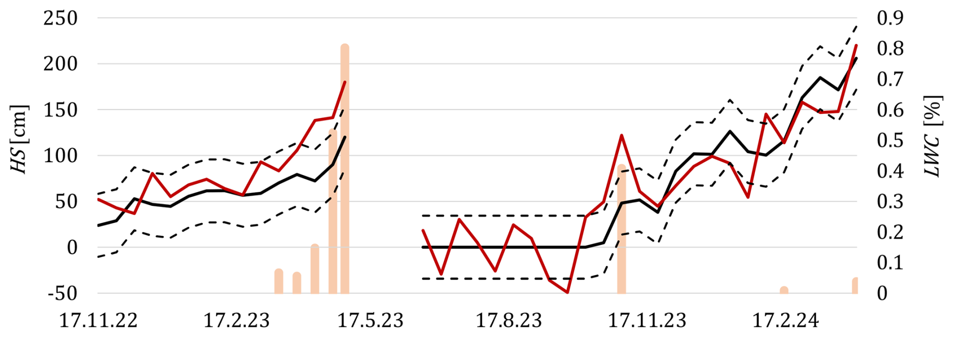
Figure A1 Comparison between HS_{mdl_LIA} (solid red line) and HS_msr (solid black line; Gessi AWS) during the two full seasons 2022/23 and 2023/24. The dotted black lines are obtained by shifting the solid one upward and downward by 31.0 cm, which is the RMSE obtained by estimating HS considering only the Gessi data. The bar chart represents the liquid water content (LWC).