Quantifying temperature-sliding inconsistency in thermomechanical coupling: a comparative analysis of geothermal heat flux datasets at Totten Glacier

Rapid sliding of ice sheets requires warm basal temperatures and lubricating basal meltwater, whereas slow velocities typically correlate with a frozen bed. However, ice sheet models often infer basal sliding by inverting surface velocity observations with the vertical structure of temperature and hence rheology held constant. If the inversion is allowed to freely vary sliding over the model domain, then inconsistencies between the basal thermal state and ice motion can arise lowering simulation realism. In this study, we propose a new method that quantifies inconsistencies when inferring thawed and frozen-bedded regions of ice sheets. This method can be used to evaluate the quality of ice sheet simulation results without requiring any englacial or subglacial measurements. We apply the method to evaluate simulation results for Totten Glacier using an isotropic 3D full-Stokes ice sheet model with eight geothermal heat flux (GHF) datasets and compare our evaluation results with inferences on basal thermal state from radar specularity. The rankings of GHF datasets based on inconsistency are closely aligned with those using the independent specularity content data. To illustrate the method's utility, we identified an overcooling inconsistency across all GHFs near the western boundary of Totten Glacier (70–72° S), a region with a bedrock canyon and fast surface ice velocities, suggesting that all GHFs are underestimated. Conversely, an overheating inconsistency exists in eastern Totten Glacier across all GHFs, indicating an overestimation of ice temperature that, in this case, is associated with a warm bias in surface temperature. Our approach opens a new avenue for assessing the self-consistency and reliability of ice sheet model results and GHF datasets, which may be widely applicable.

1 Introduction

Ice sheet models are an important tool for projections of ice sheet mass balance and their contribution to sea level rise. Ice sheet models are usually initialized by “spin-up” or data assimilation such that they reproduce the present-day geometry or surface velocity of an ice sheet (Seroussi et al., 2019). Often ice sheet model simulations derive ice dynamics using ice temperatures taken from other studies (e.g., Gillet-Chaulet et al., 2012; Cornford et al., 2015; Pittard et al., 2016; Siahaan et al., 2022). In thermo-mechanically coupled ice sheet simulations, the ice sheet model is usually spun up with idealized temperature-depth profiles and then run in a thermo-mechanically coupled mode constrained by geothermal heat flux (GHF) and surface ice temperature fields (Seroussi et al., 2019). While advances in satellite and field observation technologies have led to a preliminary consensus on ice sheet geometry and surface ice temperature, significant uncertainties persist in basal boundary conditions, including GHF and basal friction, since reliable observational data are scarce. These basal properties introduce significant uncertainty in the simulated ice sheet dynamics, and thus ice sheet mass balance.

The GHF, the heat flow from the Earth's crust to the base of ice sheet, is a critical variable in the basal boundary condition for simulating the ice temperature profile, and hence ice rheology and flow dynamics (Fisher et al., 2015; Smith-Johnsen et al., 2020; Reading et al., 2022). Several GHF datasets exist, derived in various ways from geophysical observations and models, and they exhibit significant variability in both spatial distribution and magnitude (e.g., An et al., 2015; Dziadek et al., 2017; Martos et al., 2017; Shen et al., 2020; Stål et al., 2021). These GHF datasets have been widely used in thermodynamic simulations of Antarctica (e.g., McCormack et al., 2022; Shackleton et al., 2023; Park et al., 2024; Van Liefferinge et al., 2018). However, assessing the GHF field accuracy is problematic because in situ measurements such as boreholes are sparse. Few studies have assessed the quality and reliability of GHF datasets over specific regions. Kang et al. (2022) employed a combination of forward model and inversion using a 3D full-Stokes ice flow model to simulate the basal thermal state in the Lambert–Amery Glacier region and evaluate different GHFs using the locations of subglacial lakes, but the constraints used were asymmetric between frozen and thawed beds, and assigned inflated reliability to the warmer GHF maps. Indirect estimates of basal conditions have used airborne radar specularity content (Schroeder et al., 2013; Young et al., 2016) as proxies for basal wetness/dryness and thermal regime (Dow et al., 2020). Huang et al. (2024) used an inverse modeling approach similar to that of Kang et al. (2022) for Totten Glacier and combined this with measured radar specularity content to derive a two-sided constraint on the basal thermal state in addition to subglacial lakes locations. However, specularity content is not yet available for many regions of Antarctica.

The basal friction field is another poorly known boundary condition in ice sheet modeling, and a key source of uncertainty in the long-term projection of ice sheets and glaciers. Although basal slip is crucial to the 3D ice flow, it is difficult to observe. Several basal sliding parameterizations have been proposed and widely used (Weertman, 1957; Kamb, 1970; Nye, 1970; Budd et al., 1979; Fowler, 1981; Schoof, 2005; Gagliardini et al., 2007; Gladstone et al., 2014; Tsai et al., 2015; Brondex et al., 2017, 2019). The linear Weertman basal sliding parameterization is the most widely used due to its simple form. Given prescribed or modelled ice temperatures and hence ice viscosity, numerous studies have inferred the spatial distribution of the basal friction coefficient over grounded ice to best match observed present-day surface ice velocities or ice sheet geometry using snapshot or time-dependent data assimilation and inverse methods (MacAyeal, 1993; Gillet-Chaulet et al., 2012; Larour et al., 2012; Pollard and DeConto, 2012; Morlighem et al., 2013; Pattyn, 2017; Albrecht et al., 2020; Lipscomb et al., 2021; Choi et al., 2023). However, such inversions typically allow the friction coefficient to vary freely to match the surface velocity observations. This can potentially lead to conflicts with the temperature field used during the inversion. For instance, relatively fast surface ice velocity may demand basal sliding in areas where the basal temperatures are below the local pressure melting point. However, many studies overlook this aspect, and use the inversion results to initialize ice sheet dynamics simulations and estimate glacier mass balance and its contribution to sea level rise (Seroussi et al., 2019; Peyaud et al., 2020; Schannwell et al., 2020; Payne et al., 2021).

For this study, we define the inconsistencies as differences between a sliding inversion and the temperature/rheology field used as an input to that inversion. More specifically, the inconsistencies are between modelled basal sliding (which is tuned to match the observed fast surface velocity during the inversion) and modelled frozen bed, and between observed slow surface velocity (which is most likely indicative of a non-slip basal condition) and modelled thawed bed. The inconsistencies originate from multiple causes, including uncertainties in GHF, surface ice temperature, ice sheet geometry, bed topography, surface velocity, ice density and incomplete ice flow mechanics.

To the best of our knowledge, there has been no study of such inconsistencies. Here we develop a novel and generally applicable method to estimate this inconsistency without relying on basal observation data. We utilize this approach to evaluate the quality of ice flow model results. Notably, this approach can also serve as a supplementary method for assessing geothermal heat flux datasets, relying solely on surface ice velocity observations rather than additional englacial or subglacial data.

We apply our method to Totten Glacier, a primary outlet of the Aurora subglacial basin in East Antarctica (Greenbaum et al., 2015; Pritchard et al., 2009). The Totten Glacier subregion experienced the largest mass loss among drainage basins in East Antarctica during the period 1979–2017 and 2003–2020 (Kim et al., 2024; Rignot et al., 2019) (Fig. 1a). We examine inconsistencies between simulated ice temperature and ice velocity fields from Huang et al. (2024) using a 3D full-Stokes model with the various GHFs, and we use this analysis to rank the reliability of different GHF fields. This GHF ranking closely resembles that reported by Huang et al. (2024), which used the agreement between the modelled basal thermal regime and specularity content, which we take as a validation of the method. Since the new method does not require any englacial or subglacial data, it can be applied to many glaciers, particularly those lacking observations. Our approach can provide a swift assessment of the plausibility of basal temperature and velocity simulated by ice sheet models. Additionally, it can be effectively utilized to map the spatial distribution of GHF over- or under-estimation.

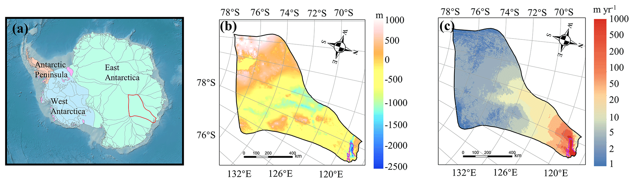
Figure 1 (a) Geographic location of Totten Glacier (red outline) in Antarctica; (b) bed elevation of Totten Glacier, the purple curve represents the grounding line; (c) observed surface velocity.

2 Method

2.1 Definition of Metrics

There is no direct correlation between basal temperature and surface velocity; rather, they are linked through the basal thermal state – the basal temperature being at or below the pressure melting point. The ice bottom in the study domain can be partitioned into thawed and frozen beds depending on whether the simulated basal ice temperature reaches the local pressure melting point. To effectively penalize models exhibiting both localized overheating (bed too warm) and overcooling (bed too cold), we establish overheating metrics within the thawed-bedded region and overcooling metrics within the frozen-bedded region to quantitatively assess the inconsistency between the simulated temperature and velocity fields. Thus, we provide two-sided constraints on the temperature field that penalize both too high and too low ice temperature.

Overcooling occurs where basal temperature is underestimated. Crucially, in regions with relatively fast observed surface velocity, the inverse method nevertheless yields a nonzero basal velocity – a physically inconsistent result given the cold basal temperature. When basal ice temperature is below the pressure melting point, the basal modelled velocity is expected to approach zero. This inconsistency is larger for faster simulated basal velocity magnitude and for colder simulated basal temperatures. We therefore use a formula that accounts for both variables to quantify overcooling:

$$\begin{array}{}\text{(1)}& \mathrm{AOC}=(T_{\mathrm{melt}}-T_{\mathrm{bm}})\times U_{\mathrm{bm}},\end{array}$$

where AOC stands for absolute overcooling, T_melt is the basal pressure melting point, T_bm represents the simulated basal ice temperature and U_bm means the simulated basal velocity magnitude.

It is not straightforward to quantify the inconsistencies between modelled thawed bed and expected slow basal velocity magnitude given slow observed surface velocity magnitude. We note the fact that modelled basal sliding velocity magnitude must remain non-negative. If the ice is warm and soft enough to permit deformation such that the modelled surface velocity magnitude is much faster than the observed, then a friction inversion will be ineffective to correct this misfit, producing a bias towards positive misfits (i.e., model velocities are too fast) in the inversion results. Therefore, we use the positive difference between simulated and observed surface velocity magnitude to calculate the inconsistency caused by the overheating effect:

$$\begin{array}{}\text{(2)}& \mathrm{AOH}=max(\mathrm{0},U_{\mathrm{sm}}-U_{\mathrm{obs}}),\end{array}$$

where AOH refers to absolute overheating, U_sm represents the modelled surface velocity magnitude and U_obs is the observed surface velocity magnitude. We only calculated AOH for the thawed-bedded areas, i.e. T_bm=T_melt, because observed surface velocity magnitude errors are proportionally much less in thawed-bedded areas (corresponding to fast flow regions) than in frozen-bedded area (correspond to slow flow regions).

To mitigate the impact of substantial differences in observed surface velocity magnitude across various areas, we also define “relative overheating” (ROH) and “relative overcooling” (ROC), dividing AOH and AOC  by the observed surface velocity magnitude respectively:

$$\begin{array}{}\text{(3)}& {\displaystyle }\mathrm{ROH}={\displaystyle \frac{max(\mathrm{0},U_{\mathrm{sm}}-U_{\mathrm{obs}})}{U_{\mathrm{obs}}}},\text{(4)}& {\displaystyle }\mathrm{ROC}=(T_{\mathrm{melt}}-T_{\mathrm{bm}})\times {\displaystyle \frac{U_{\mathrm{bm}}}{U_{\mathrm{obs}}}}.\end{array}$$

2.2 Normalization and ranking

Overheating and overcooling inconsistencies are calculated on thawed bed and frozen bed, respectively. To evaluate the inconsistencies for the whole domain, we linearly normalized the overheating inconsistency and overcooling inconsistency to range from zero to one and then sum them as:

$$\begin{array}{}\text{(5)}& {\displaystyle }\mathrm{ACI}=L_{\mathrm{N}}\left(\mathrm{AOC}\right)+L_{\mathrm{N}}\left(\mathrm{AOH}\right),\text{(6)}& {\displaystyle }\mathrm{RCI}=L_{\mathrm{N}}\left(\mathrm{ROC}\right)+L_{\mathrm{N}}\left(\mathrm{ROH}\right),\end{array}$$

where ACI means absolute combined inconsistency, RCI represents relative combined inconsistency, and L_N represents linear normalization. Taking AOC as an example, its linear normalization is:

$$\begin{array}{}\text{(7)}& L_{\mathrm{N}}\left(\mathrm{AOC}\right)={\displaystyle \frac{\mathrm{AOC}-{\mathrm{AOC}}_{\min }}{{\mathrm{AOC}}_{\max }-{\mathrm{AOC}}_{\min }}}.\end{array}$$

Therefore, we obtain three absolute inconsistencies (AOH, AOC, ACI) and three relative inconsistencies (ROH, ROC, RCI), with which we can comprehensively analyze the temperature-sliding inconsistency in the inversion results of ice sheet model. For each metric, we rank the eight GHF datasets from one (least inconsistent) to eight (most inconsistent). The final score for each dataset is the average of its ranks across the six metrics to ensure a comprehensive evaluation, as a reasonable simulation result should perform well across thawed bed, frozen bed, and the whole region. We only consider grounded ice and exclude points located at the domain boundary due to relatively poor model performance there.

The specific metrics that we use to quantify this inconsistency could be adaptable, for example by using a squared error term instead of the linear error terms that we used. However, the general practice of emphasizing and quantifying the inconsistency between a sliding inversion and the temperature/rheology field used as an input to that inversion is novel.

2.3 Methodology in Huang et al. (2024)

In this study, we validate our method by comparing our ranking of GHF datasets to the observationally constrained ranking established by Huang et al. (2024). For readers not familiar with this paper, we provide here a brief summary of their method and, in the next section, clarify the distinction between their paper and the present study.

Huang et al. (2024) employed thermo-mechanical coupled simulations using eight GHF datasets to investigate the steady-state thermal regime of Totten Glacier. The methodology comprised two interconnected modeling components:

1. Forward Modeling: An enhanced shallow-ice approximation model integrated with a subglacial hydrology module was utilized to simulate englacial temperature profiles.

2. Inverse Problem: A full-Stokes ice flow model was applied to resolve the basal friction coefficients through inverse analysis, to minimize the misfit between simulated and observed velocities while simultaneously generating velocity predictions.

A feedback loop was then established: the velocity outputs from the inverse model were used to refine key parameters in the forward model – specifically constraining the basal slip ratio, rheological properties, and shape functions. This bidirectional coupling process underwent multiple iterations to achieve convergent steady-state solutions.

Huang et al. (2024) utilized radar specularity content data to differentiate localized wet (thawed) versus dry (frozen) basal conditions and used this data as a two-sided constraint on the basal thermal state. They compared modeled basal thermal states derived from different GHFs to evaluate the reliability of the GHF datasets.

2.4 Distinction from Huang et al. (2024)

In Huang et al. (2024), modelled surface velocities are compared with observations over the whole domain during the inversion for basal parameters for each GHF dataset. Here, surface velocities act as the observational constraints for the mechanical inversion.

Although the overheating metrics here use the surface velocities and can thus be considered a subset of the inversion residual, our overcooling metrics are based on the basal sliding velocity derived from the inversion, which is not part of the mechanical inversion's residual. A mechanical inversion does not take into account the physical plausibility of the sliding result it produces. Therefore, it is not circular reasoning to compare two different parts of a model to each other; rather, it is an assessment of internal consistency, or lack thereof. A mechanical inversion may fit the surface velocity observations equally well when forced with many different models of the ice sheet thermal structure and rheology; however, if some models require high sliding velocities in frozen-bedded regions, then they should be downweighted in comparison to models that show a good agreement between basal temperature and velocity.

The method here does not require any additional observations beyond the surface velocities used in the mechanical inversion. However, there are “independent constraints” in the method here, which are not observations, but rather a priori physical understandings that: (1) rapid sliding requires warm basal temperatures and subglacial water; (2) reducing the basal slip coefficient cannot prevent the ice from flowing by internal shear deformation. The inconsistency metrics developed in this paper are an attempt to quantify and rank the extent to which these basic (and uncontroversial) physical understandings are violated.

3 Application to Totten Glacier with Different GHFs

3.1 Study domain and Data

We apply our method to evaluate simulated ice temperature and ice velocity in Totten Glacier with eight GHF datasets by Huang et al. (2024). Huang et al. (2024) used the present-day surface ice temperature (Le Brocq et al., 2010a), observed surface velocity from MEaSUREs InSAR-Based Antarctic Ice Velocity Map, version 2 (Rignot et al., 2017) and ice sheet topography data from BedMachine Antarctica, version 2 (Morlighem et al., 2020). The eight GHF datasets were derived by various methodologies, resulting in significant differences in both spatial distribution and magnitude (Fig. 2). GHF fields from Stål et al. (2021), Haeger et al. (2022), Lösing and Ebbing (2021) and Martos et al. (2017) generally exhibit higher magnitudes than the other GHFs. Supplement Table S1 summarizes the input datasets, which follow the configuration described in Huang et al. (2024).

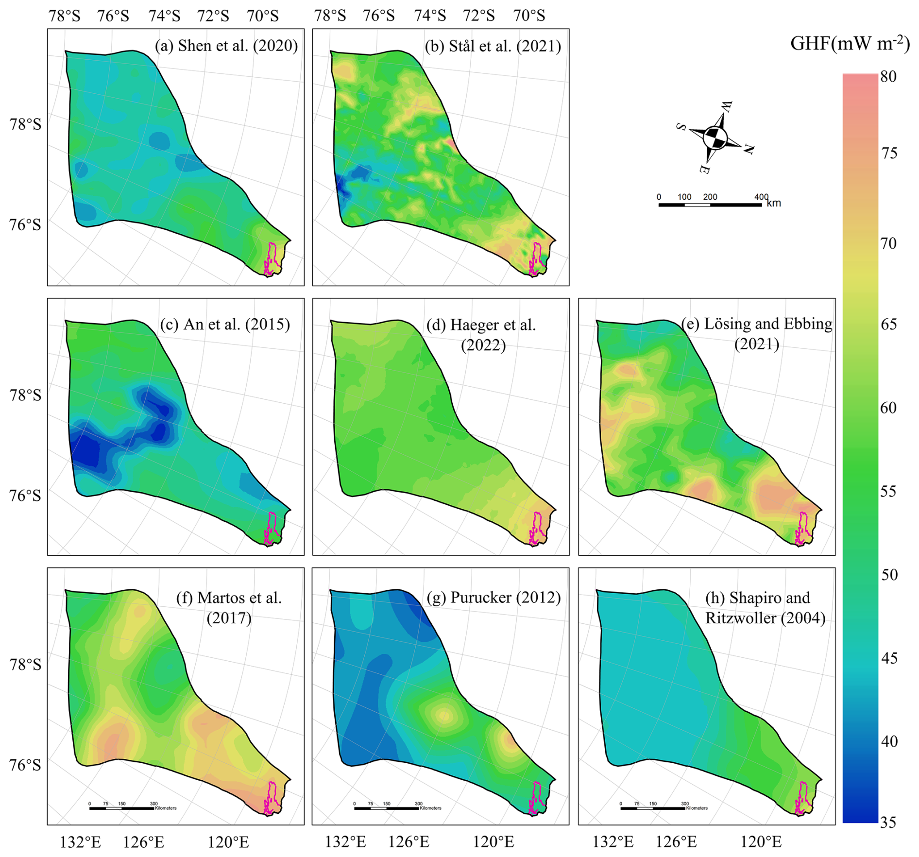
Figure 2 The spatial distribution of the eight GHF datasets for Totten Glacier (a–h) used as input data in Huang et al. (2024). The purple line depicts the grounding line.

The spatial distribution of modelled basal temperature using the eight GHFs displays both similarities and heterogeneity. In the northern part of Totten Glacier, there is a consistent thawed-bedded pattern across all eight simulation results (Fig. S1 in the Supplement), which originates from the grounding line and extends upstream to approximately 71° S. This thawed-bedded area is not contiguous with the lateral boundaries of Totten Glacier but is instead bordered by frozen bed. All eight GHF datasets produce low basal ice temperatures in the inland southwest, with Purucker (2012), Shapiro and Ritzwoller (2004), Shen et al. (2020) and Lösing and Ebbing (2021) being colder than the other four GHF products. The basal ice velocities modelled from the eight different GHF datasets produce similar spatial distributions (Fig. S2), which can be expected as they were derived using the same inverse method and constrained by the identical observed surface ice velocity. The modelled basal ice velocity is fast near the grounding line and its upstream area. There are also high velocities between 70 and 72° S close to the western boundary of Totten Glacier, which are associated with subglacial canyon features in the basal topography (Fig. 1b) and observed fast surface ice velocity there (Fig. 1c).

3.2 Spatial Distribution of Inconsistencies with one GHF dataset

In this section, we show the spatial fields of the inconsistency metrics (Sect. 2.1 and 2.2) for the modelled result in Huang et al. (2024), using Martos et al. (2017) GHF as an example. This example illustrates the interpretation process before conducting a comprehensive comparative analysis for the result with eight GHF datasets.

The modelled result based on the Martos et al. (2017) GHF reveals extensive regions of thawed bed with limited areas of frozen bed. The frozen bed is predominantly located in the southern corner of the study domain, where the modelled basal velocity magnitude approaches zero, consistent with cold basal ice temperature. Consequently, the AOC inconsistency at this marginal zone is negligible (Fig. 3). Along the western margin of Totten Glacier, basal ice temperature remains below the pressure melting point, albeit approaching it. However, localized regions exhibit high basal velocities of several tens of meters per year, contradicting the presence of a frozen bed and resulting in large AOC inconsistencies.

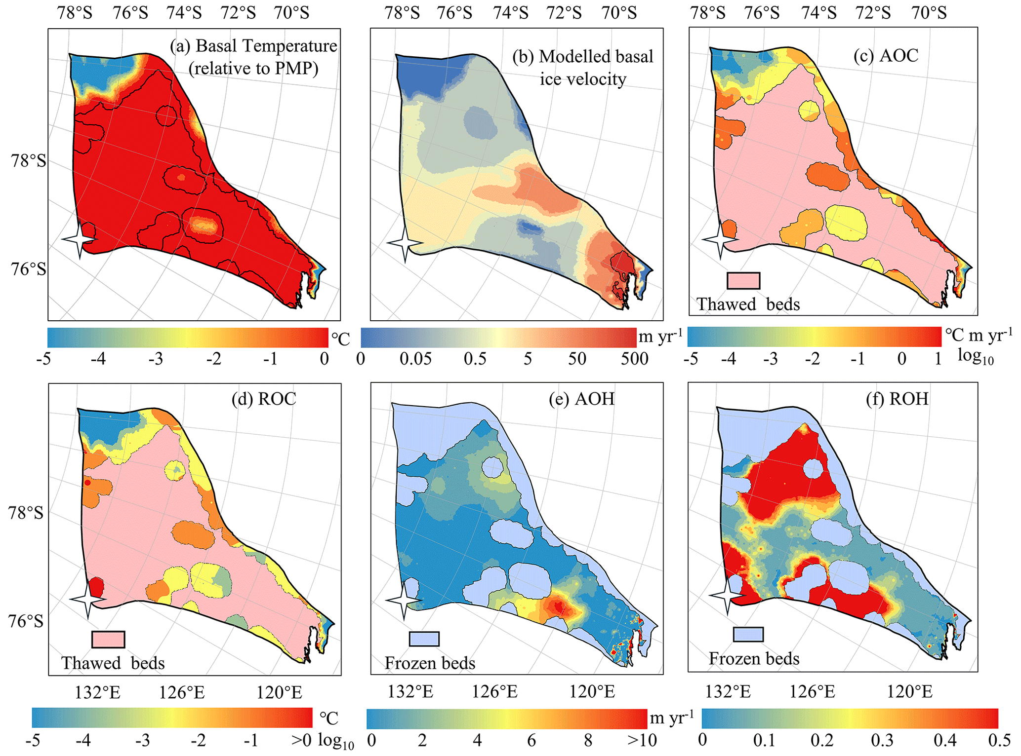
Figure 3 Spatial distribution of modelled basal ice temperature (a), modelled basal ice velocity magnitude (b), AOC (c), ROC (d) inconsistencies in modelled frozen-bedded regions, and AOH (e) and ROH (f) inconsistencies in modelled thawed-bedded regions associated with Martos et al. (2017) GHF. The colormap in (c) and (d) is on logarithmic scale. The pink region in (c) and (d) represents modelled thawed bed, while the blue region in (e) and (f) indicates frozen-bedded areas. The white star represents Dome C.

Conversely, large AOH values are observed between 69 and 71° S in the eastern Totten Glacier region, where the simulated surface velocity magnitude exceeds observational data by > 5 m yr⁻¹ (Fig. 3e). In this area, the modelled basal ice temperature reaches the pressure melting point, with the modelled basal velocity magnitude at approximately 0.05 m yr⁻¹. Basal friction inversion failed to reproduce observed surface velocity magnitude due to the model's overestimation of ice temperature and softness. This pronounced velocity mismatch highlights a fundamental inconsistency in the eastern glacier region, likely originating from discrepancies in the input datasets. Regions of high ROH and ROC values coincide with areas of relatively high AOH and AOC, particularly where the observed surface velocities are slow, as per their formulations.

3.3 Spatial Distribution of Inconsistencies with eight GHF datasets

3.3.1 Overcooling Inconsistency on Frozen Beds

We calculated the inconsistency metrics for the thawed and frozen beds respectively, and summed the values over the corresponding regions. The results are shown in Table 1. To visualize the spatial heterogeneity of these inconsistencies, we mapped the distribution of the metrics. The spatial distribution of AOC reveals that most GHF datasets exhibit significant local overcooling inconsistencies at the subglacial canyon between 70 and 72° S (Fig. 4). There is fast basal sliding in the inverse model results (Fig. S2), however, the modelled basal ice temperatures inferred from most of the GHF datasets are below the pressure melting point (Fig. S1). High specularity content in radar data (Fig. 4c) suggests the presence of basal water in the subglacial canyons here (Dow et al., 2020; Huang et al., 2024), which also suggests that the basal ice temperature should be at the pressure melting point and confirms the inconsistency between the modelled temperature and velocity fields.

Table 1 Summary of inconsistency metrics for different GHF maps.

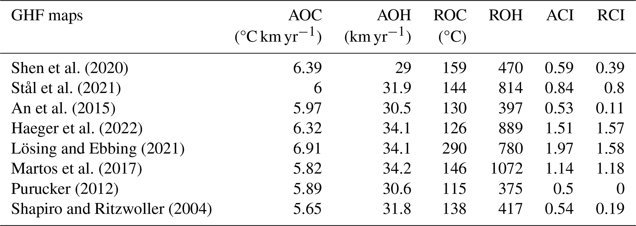
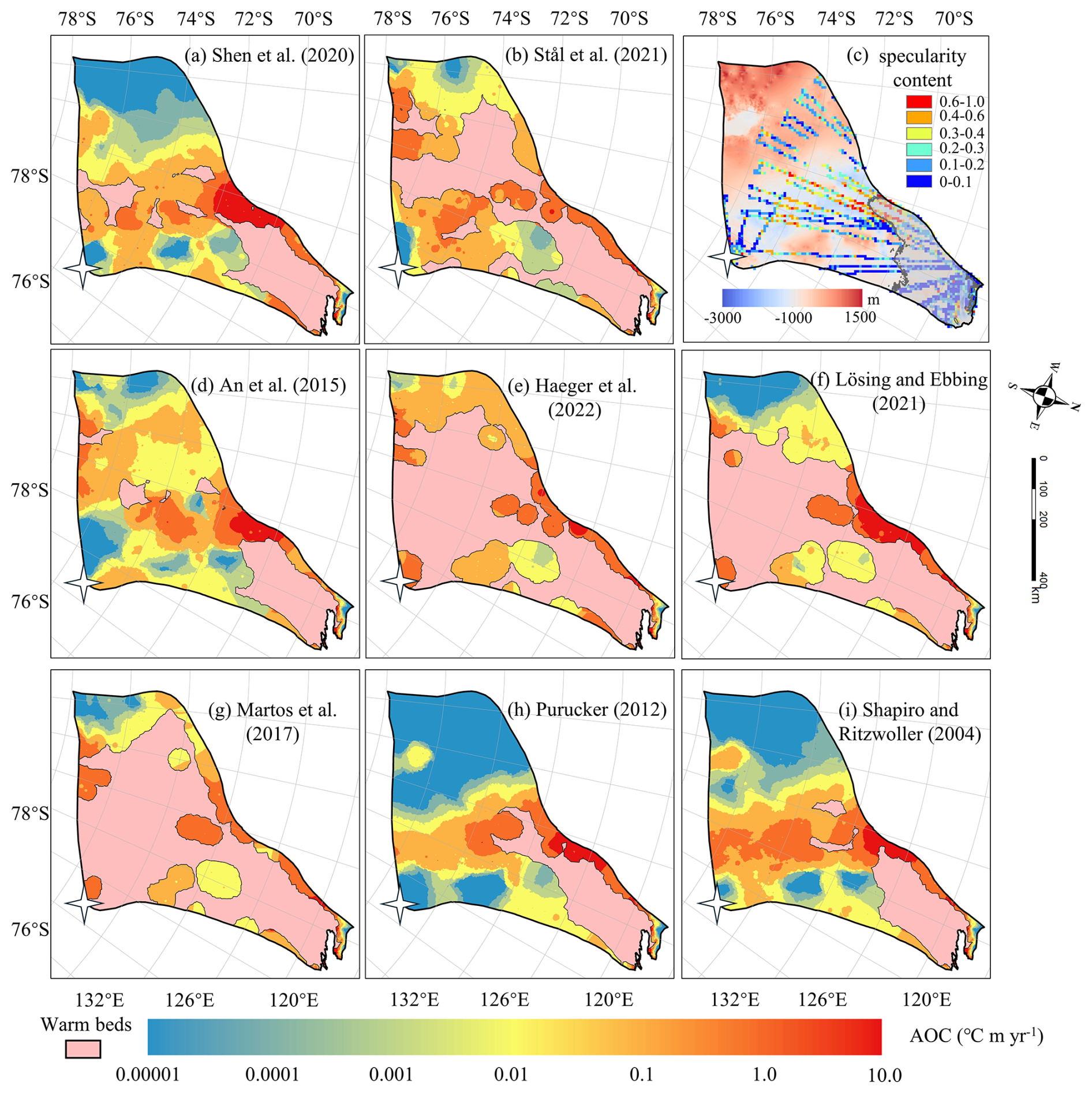
Figure 4 Spatial distribution of AOC inconsistency in modelled frozen-bedded regions (a)–(b) and (d)–(i) associated with the GHFs (a–h) in Fig. 2. The pink region represents modelled thawed bed. (c) Specularity content sourced from radar data collected by ICECAP (Dow et al., 2020) with the bed elevation in the background. Gray area in (c) corresponds to surface velocity magnitude exceeding 30 m yr⁻¹. The white star represents Dome C. Note the colormap is logarithmic.

The area near the grounding line is characterized by fast ice flow (Fig. S2) and thawed bed (Fig. 4), yet some of the margin is frozen-bedded with modelled basal temperature below the pressure melting point, resulting in high AOC. Overall, modelled results with most GHF datasets show small overcooling inconsistencies. The modelled results using GHF from Purucker (2012), Shapiro and Ritzwoller (2004), Shen et al. (2020), Lösing and Ebbing (2021) exhibit no overcooling inconsistency in southwestern Totten Glacier (Fig. 4). The largest value of ROC across most GHF occurs at Dome C (white star in Fig. 5), where the observed surface ice velocity magnitude is close to zero (Fig. 1c).

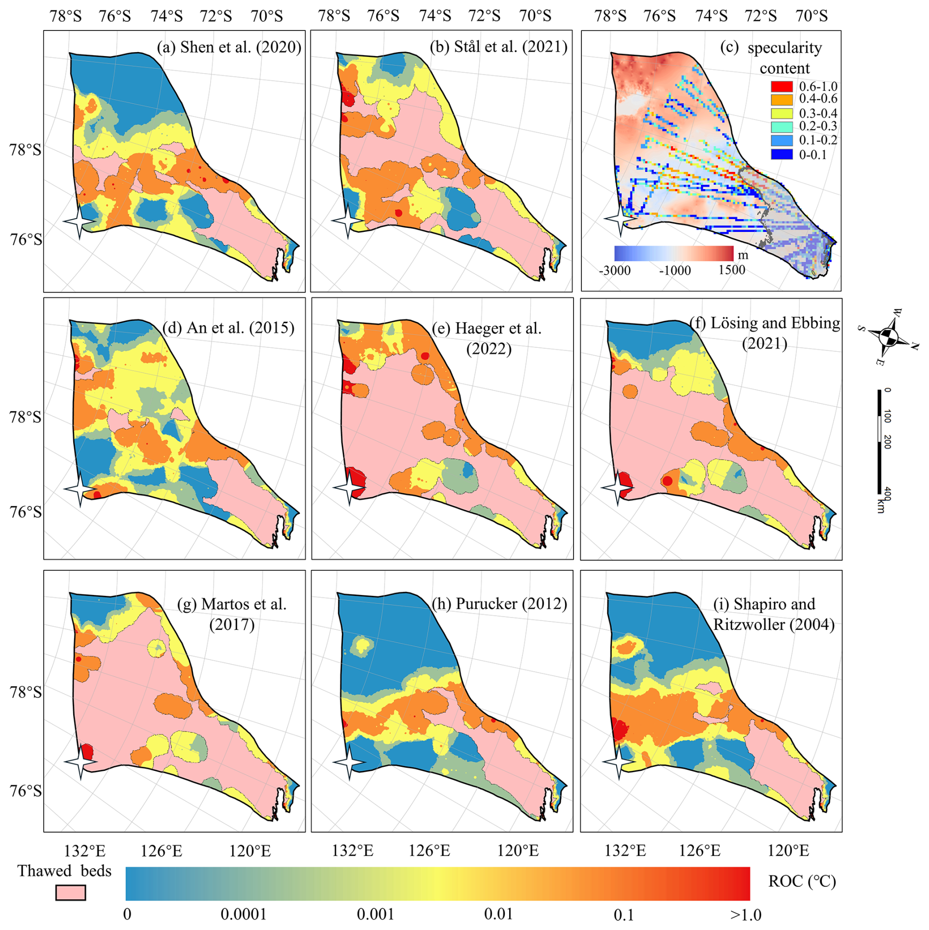
Figure 5 The spatial distribution of relative overcooling (ROC) inconsistency in frozen-bedded regions with (a), (b) and (d) to (i) corresponding to the GHFs (a–h) in Fig. 2. The pink area represents the thawed beds. Dome C is marked by a white star. (c) Locations of specularity content derived from radar data collected by ICECAP (Dow et al., 2020) and with the bed elevation in the background. The gray curve is the contour of the surface velocity magnitude of 30 m yr⁻¹. Note the colormap is logarithmic.

3.3.2 Overheating Inconsistency on Thawed Beds

The simulations with all eight GHFs yield similar spatial distributions of AOH (Fig. 6) on the common area of thawed bed, and similar locations of high AOH values. A common high AOH area is located between 69 and 72° S in the eastern part of Totten Glacier, due to simulated surface ice velocities greatly exceeding the observed surface ice velocities. Low specularity content from radar data (Fig. 6c) suggests there is no basal water in the area (Dow et al., 2020; Huang et al., 2024). Therefore, it is likely that the basal ice temperature is overestimated there. The simulations with all the eight GHFs also yield similar spatial distribution of ROH (Fig. 7), but its largest values are mostly in the slow flowing region as one may expect from its formulation (Eq. 3).

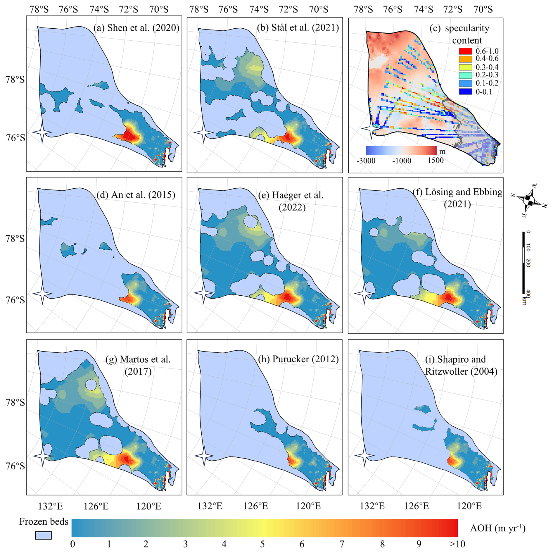
Figure 6 Spatial distribution of AOH in thawed-bedded regions with (a)–(b) and (d)–(i) corresponding to the GHFs (a–h) in Fig. 2. The blue region indicates frozen-bedded areas. (c) Locations of specularity content, same as Fig. 4c. The white star represents Dome C.

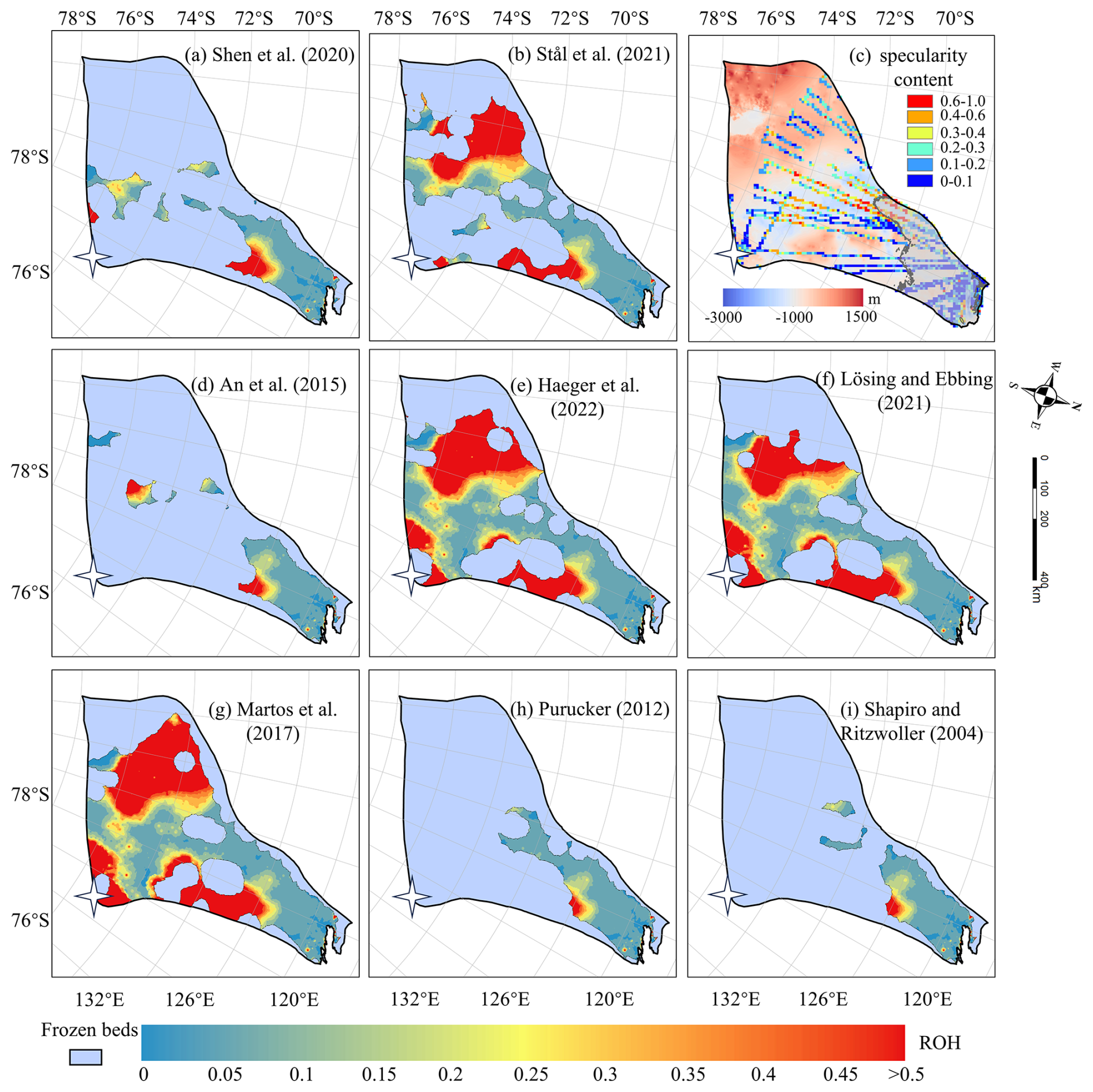
Figure 7 The spatial distribution of relative overheating (ROH) inconsistency in thawed beds with (a), (b) and (d) to (i) corresponding to the GHFs (a–h) in Fig. 2. The blue mask represents the frozen beds. (c) Locations of specularity content (coloured points), same as Fig. 6. The white star represents Dome C.

3.4 Evaluation of Model Inconsistency with Eight GHFs

To assess the overall inconsistency of each geothermal heat flux dataset, we calculate the sum of each metric over all points. All inconsistency indices for the simulation results using the eight GHF datasets are illustrated in Fig. 8. The overheating inconsistency associated with Purucker (2012) and Shapiro and Ritzwoller (2004) GHFs is predominantly localized in fast-flowing regions. Consequently, after normalization by the observed surface velocity magnitude, their relative rankings improve (Fig. 8). The GHFs from Purucker (2012), An et al. (2015), Shapiro and Ritzwoller (2004), and Shen et al. (2020) demonstrate balanced performance with respect to both overheating and overcooling inconsistency metrics, thereby securing the top four positions in both ACI and RCI. Their ACI values exhibit similarity, ranging from 0.50 to 0.59 (Fig. 8c). In contrast, simulation result utilizing Martos et al. (2017) GHF exhibits low AOC but high AOH. Simulation results utilizing Stål et al. (2021) GHF show low ROC but relatively high ROH. Notably, simulation results employing GHFs from Martos et al. (2017), Haeger et al. (2022), and Lösing and Ebbing (2021) demonstrate comparably high AOH values. These four GHF datasets – Martos et al. (2017), Stål et al. (2021), Haeger et al. (2022), and Lösing and Ebbing (2021) – are ranked in the bottom four positions for both ACI and RCI metrics. Furthermore, the ranking order of the eight GHFs remains consistent between ACI and RCI.

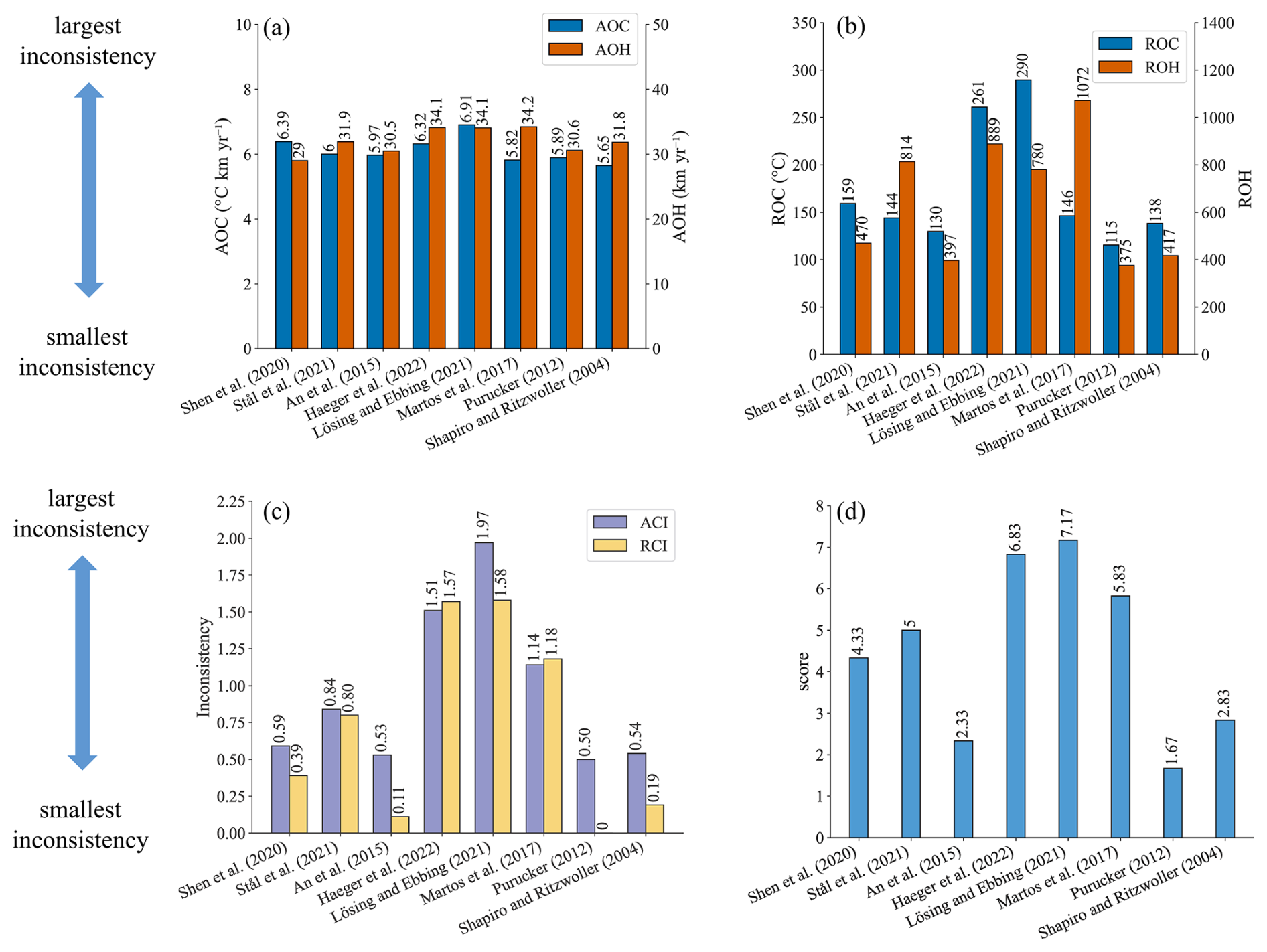
Figure 8 Six inconsistency indicators and the final ranking of eight GHF datasets. (a) The absolute overcooling and overheating inconsistencies, AOC and AOH; (b) the relative overcooling and overheating inconsistencies, ROC and ROH; (c) the absolute and relative combined inconsistencies, ACI and RCI; (d) the average of ranking scores from one to eight using the six inconsistency indicators. The values of inconsistencies and scores are labeled at the top of the bars.

The final averaged ranking (Fig. 8d) across the indices is also the same as that of ACI and RCI. Purucker (2012), An et al. (2015) and Shapiro and Ritzwoller (2004) GHFs occupy the top three positions. Following closely, Shen et al. (2020) and Stål et al. (2021) GHFs secure the 4th and 5th positions, respectively. Martos et al. (2017), Haeger et al. (2022) and Lösing and Ebbing (2021) GHFs are ranked as the bottom three among the eight GHFs in Totten Glacier. The thermal state produced by the optimal GHF result shows that thawed beds predominantly cluster around the grounding line and its upstream regions. Conversely, the inland areas of Totten largely exhibit cold temperatures, with relatively sparse thawed-bedded areas.

4 Discussion

4.1 Sensitivity of Inconsistencies to GHF Datasets

Comparing the GHF dataset rankings between this study and Huang et al. (2024), we find that the top four and the bottom four are the same in the two studies, albeit with slight variations in ranking. The lower ranking of Shen et al. (2020) in this study may be attributed to several factors. Firstly, Huang et al. (2024) excludes areas with ice velocity magnitude exceeding 30 m yr⁻¹ (Fig. 4c) because specularity content is an ambiguous indicator of wet beds there. Secondly, the GHF from Shen et al. (2020) yields higher basal temperature and also faster basal ice velocities in most of the frozen bed of Totten Glacier, hence exhibits greater overcooling inconsistency, compared with Purucker (2012), leading to a decrease in its rankings (Fig. S3). Lastly, Huang et al. (2024) primarily relied on specularity content, while our study evaluated datasets based on inconsistencies in the simulation results. Despite these methodological differences, both studies identified four relatively well-performing GHF datasets for Totten Glacier, which exhibit similar distributions of thawed and frozen beds when compared to the other four datasets (Fig. 4 and Fig. 6). This similarity underscores that the thawed bed is concentrated near and upstream of the grounding line. Datasets from Stål et al. (2021), Martos et al. (2017), Haeger et al. (2022), and Lösing and Ebbing (2021) exhibit a tendency to overestimate GHF in central Totten Glacier.

Simulations employing GHF datasets from Stål et al. (2021), Martos et al. (2017), Haeger et al. (2022), and Lösing and Ebbing (2021) yield more extensive thawed-bedded regions and are expected to exhibit greater overheating inconsistency. Nevertheless, these models also exhibit relatively high overcooling inconsistency despite the limited extent of frozen-bedded regions. We quantified the discrepancies between these four GHF datasets and the Purucker (2012) GHF in terms of modelled basal velocity, basal temperature relative to the pressure melting point, and AOC (Fig. S4). The Purucker (2012) GHF yields lower basal ice temperatures and slower basal velocities across most frozen-bedded regions, consequently resulting in lower AOC values compared to the other four GHF datasets.

4.2 Causes of Inconsistencies and Sources of Uncertainty

We have developed an indirect method that utilizes surface velocity observations to assess the quality of simulated basal temperature. However, the mere fact that inconsistencies exist does not by itself tell us what caused those inconsistencies. Broadly speaking, the measured inconsistencies can come from two sources: temperature or velocity. Uncertainties in any of the input datasets used to compute those two fields can produce inconsistencies, as can simplifications in the model physics. Here, we have tested the influence of one particular boundary condition, GHF, since that field is particularly hard to constrain. Because all other inputs are kept constant, the differences in the inconsistencies that we calculated between different simulations can be attributed to the GHF fields. However, we also found that all of the models we tested had non-zero inconsistency (Figs. 4, 6). The absolute inconsistencies, AOH and AOC, had particularly small between-model variability in comparison to their mean value. This could be related to uncertainties or limitations in the input GHF fields, but it may also indicate sensitivities to other model inputs. For instance, the surface temperature used in Huang et al. (2024) represents the present-day climate, but the thermal structure of the ice sheet may reflect colder temperatures during the last glacial cycle. We discuss an additional experiment we performed to test the influence of uncertainty in surface temperature on our inconsistency metrics in Sect. 4.3 below. While the cooler surface temperatures during the glacial period exerted a cooling effect on ice sheet temperature, lower surface accumulation rates over the same period induced a warming effect. Uncertainties in bed topography should influence both our thermal and our mechanical models, with deeper ice being more likely to be warm, and with errors in ice thickness producing compensating errors in basal sliding in our mechanical inversion. In the study of Huang et al. (2024), BedMachine v2 was used for ice thickness and subglacial topography. However, Bedmap3 (Pritchard et al., 2025) has better-resolved mountains and smoother trough margins.

The simulation results we use from Huang et al. (2024) came from a 3D isotropic full-Stokes ice flow model. While full-Stokes is generally considered an ice sheet model with the most complete physical processes to date, the use of an isotropic rheology may not be valid in some parts of the ice sheet, such as near ice divides or at the margin of an ice stream where the history of past ice deformation creates anisotropic crystal fabric that affects the present-day mechanical properties (Martín et al., 2009; Zhao et al., 2018; Zwinger et al., 2014). Isotropic flow laws often require the use of an “enhancement factor” for vertical shear in the lower part of the ice column, an ad hoc correction that would have a particularly large influence on our computed overcooling metrics. Thus the isotropic flow law potentially introduces errors in modelled strain rates and, hence, bias in basal sliding velocities obtained by inversion methods (Budd and Jacka, 1989; Gerber et al., 2023; Rathmann and Lilien, 2022). Simulated surface ice velocities can be influenced by other factors in addition to ice fabric; shear margins are also impacted by accumulated rupture, such as damage along a shear margin (e.g., Benn et al., 2022; Lhermitte et al., 2020; Schoof, 2004; Sun et al., 2017). Ice deposited during the last glaciation has different chemistry (especially concentrations of chloride and possibly sulphate ions) which leads to smaller crystals that develop a strong, near-vertical, single-maximum fabric (Paterson, 1991). However, ice fabric data is sparse, known from direct observations at ice cores (Azuma and Higashi, 1985) or inferred from specialized radar measurements (Fujita and Mae, 1994; Jordan et al., 2022), and its impact is beyond the scope of this study as we refrain from incorporating additional observational data relying only on widely-available surface ice velocities.

Our inconsistency metrics are designed to provide bidirectional constraints, wherein the model is penalized for both overheating and overcooling. By adopting this bidirectional constraint framework, we aim to mitigate the risk of unidirectional constraints leading to excessively cold or warm outcomes being deemed optimal. However, our inconsistency metrics only provide a bidirectional constraint when viewed in a spatially integrated sense. Locally, we only have unidirectional constraints. This is because our overheating metrics are only computed where the bed is at the melting point, and our overcooling metrics are only computed where the bed is below the melting point. This makes methodological sense, as sliding is generally expected to occur where the bed is thawed. However, in reality it is entirely possible that some of the areas where the modelled bed reaches the pressure melting point are still too cold (the modelled melt rate is lower than the real melt rate), and conversely, it is also possible that some of the areas where the modelled bed is below the pressure melting point are still too warm (the real temperature is colder still). Our method cannot identify these areas. Thus, our inconsistency metrics may underestimate variability in the ice sheet thermal state: we have no way to penalize frozen regions that are not cold enough or thawed regions that are not warm enough. We leave the development of these constraints to future work.

4.3 Impact of Input Datasets

There is a common area between 69 and 72° S in the eastern part of Totten Glacier with the largest AOH (Fig. 6) for all the GHFs varying from 48 to 70 mW m⁻², which suggests that the AOH inconsistency is from other ice sheet properties rather than GHF. Zhang et al. (2022) reconstructed Antarctic near-surface air temperature based on MODIS land surface temperature measurements and in situ air temperature records from meteorological stations from 2001 to 2018. We compared the reconstruction of near-surface air temperature in the year 2001 (Zhang et al., 2022) and the ALBMAP v1 dataset used in Huang et al. (2024). The surface air temperature in the area with large AOH from ALBMAP v1 is 0.6–3.1 °C higher than that from the reconstructed near-surface air temperature in 2001 (Fig. 9). The MODIS-based near-surface air temperature product shows warming in Totten Glacier from 2001 to 2018. Even so, the surface air temperature in the area with large AOH from ALBMAP v1 is still higher than that in 2018 but over a smaller area. Therefore, we infer that the large AOH may be attributed to a warm bias in the present-day ice surface temperature derived from ALBMAP v1 in this area. The englacial temperature will be lower than present-day ice sheet surface temperature used in the model but warmer than the average surface temperature during the last glacial-interglacial cycle. We lowered the surface ice temperature in this area by 1 °C, reran the simulation, and found that AOH with all the GHFs was halved (Fig. 9e).

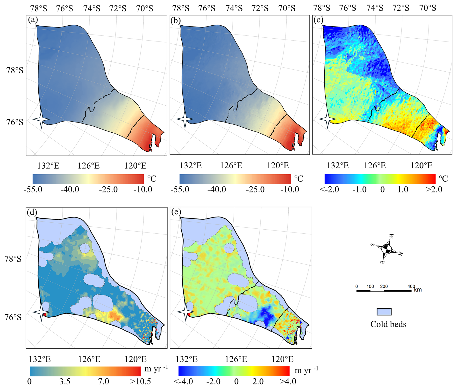
Figure 9 Surface ice temperature from ALBMAP v1 (a) and MODIS-based near-surface air temperature (b) in the year 2001, and their difference (c). (d) The AOH using modified surface ice temperature by reducing the temperature between the two black lines (contour lines of −44 and −26 °C) in (a) by 1 °C and GHF of Martos et al. (2017). (e) The difference between the AOH using cooler surface ice temperature and the original AOH. The white star represents Dome C.

4.4 Implications for Ice Sheet Dynamics

While evaluating inconsistencies highlights the spatial distribution of mismatches, it does not inherently elucidate their underlying causes. The primary factors to investigate are surface temperature, GHF, accumulation rate, and ice thickness, representing the most critical boundary conditions. Furthermore, integrating multiple sources of prior knowledge can help constrain model parameters:

1. High-resolution radar measurements: The availability of ice thickness data along flight lines should be assessed to validate geometric boundary conditions.

2. Paleoclimate context: Historical climate reconstructions indicate significantly colder surface temperatures during glacial periods compared to present-day conditions, with correspondingly lower accumulation rates. These paleo-temperature conditions likely induced a long-term thermal memory within the ice column, potentially contributing to observed discrepancies between modeled and measured basal properties.

Therefore, we recommend a systematic evaluation of: (1) The spatial distribution of radar-derived ice thickness measurements; (2) The temporal consistency of surface temperature boundary conditions; (3) The sensitivity of model results to GHF variations; (4) Accumulation rate reconstructions during key climatic periods. This multi-faceted approach helps isolate the causes of inconsistencies in ice sheet simulations.

Given that data assimilation and inverse methods are widely employed to infer basal friction coefficients in ice sheet simulations, it is essential to acknowledge the impact of the inconsistencies identified in our study on ice sheet dynamics. A frozen bed is supposed to provide substantial resistance and limit basal sliding; however, if the basal temperature is overestimated, it may decrease viscosity and enhance basal sliding. This overheating inconsistency would lead to an overestimation of ice flow speeds, discharge, and dynamic ice loss (Artemieva, 2022; Burton-Johnson et al., 2020). Similarly, underrepresentation of thawed bed conditions will lead to an underestimation of ice discharge and, consequently, an underestimation of ice sheet's response to climate warming. The basal thermal regime critically influences the stability of grounding lines and the behavior of ice streams (Dawson et al., 2022; Robel et al., 2014). In a warming climate, increases in geothermal or frictional heating can trigger basal thawing in these areas, lowering basal friction and potentially initiating rapid grounding line retreat – a key component of marine ice sheet instability (MISI) (Reese et al., 2023; Ross et al., 2012). Without incorporating a self-consistent thermal model into the inversion, projections may misrepresent the onset and extent of these dynamic instabilities. Our findings underscore that a fully coupled inversion framework would use not only surface velocity data but also incorporate direct or proxy observations of basal temperature and subglacial hydrology. Such an approach would better constrain the basal friction coefficient in a physically consistent manner, reducing the risk of producing nonphysical states. This integration is especially critical for projections of ice sheet evolution under future climate change scenarios, as the dynamic response is sensitive to even small changes in basal conditions.

5 Conclusion

We propose a novel and rapid method to quantify the inconsistencies between modelled basal ice temperature and observed surface velocity magnitude and assess the quality of ice sheet model simulation results without using subglacial observation data. By using the ice temperature field to compute the rheology structure needed for a mechanical inversion and then quantifying the inconsistency between the inverted velocity field and the original ice temperature field, we are able to use remotely sensed surface velocity observations as a means to assess the quality of modelled basal temperatures. Given the challenges in acquiring subglacial data, our method can provide a streamlined and effective approach to evaluation.

We apply this method to evaluate the steady-state simulation results of Totten Glacier presented by Huang et al. (2024), which were derived using a 3D full-Stokes model with eight different GHF datasets. Assuming the inconsistencies are mainly due to quality issues of GHF datasets, we use the inconsistencies to assess the reliability of those GHF datasets. We compare our GHF ranking with that by Huang et al. (2024) which used specularity content to derive a two-sided constraint on the basal thermal state. We find that the top four and the bottom four GHFs are the same in the two studies, albeit with slight variations in ranking. Furthermore, we find that the simulations with all GHF datasets underestimate the basal ice temperature in a canyon on the western boundary of Totten Glacier, and we infer that the common high overheating inconsistencies with all the GHF datasets in the eastern Totten Glacier between 69 and 72° S may be attributed to a warm bias in the prescribed surface ice temperature used in the model. While we demonstrate that this approach works on simulation results for Totten Glacier, testing of the method on other glaciers would be useful to assess if the approach is worthwhile for revealing ambiguous conflicts in observations and simulations.