Empirical evidence of overestimated Ku-band sea ice radar freeboards in satellite altimetry

Pan-Arctic sea ice thickness estimates are routinely produced from Ku-band radar altimetry observations. State-of-the-art waveform retracking algorithms rely on the uncertain assumption that Ku-band radar waves penetrate through the snow and that the dominant return originates from surface scattering at the snow/ice interface. However, growing evidence suggests that Ku-band radar altimetry freeboards may not always accurately trace the snow/ice interface elevation. We investigate this by analyzing the evolution of spaceborne radar and laser freeboards over immobile regions of landfast first-year ice (FYI) and multi-year ice (MYI) off Greenland's coast from mid-winter to mid-summer 2022. Our results suggest that the radar freeboards over FYI trace the snow/ice interface during most of the cold season (up to mid-May, at this location), providing empirical support for the validity of the assumption of full snow penetration and a dominant return from the snow/ice interface at Ku-band frequency. Over MYI, the retracked heights correspond to locations well below the air/snow interface most of the time, at least 40 % deep in the snow but likely much deeper, although the exact depth could not be reliably assessed. However, these data also provide evidence for short periods of positively biased Ku-band radar freeboards throughout the winter and the melt season. In particular, our results suggest that, during winter, the Ku-band radar freeboards tend to be biased high (i) for ice with a saline snow cover during a warming event (brine volume > 1 %), and (ii) during and immediately after strong snowfall events. Winter warming events are often accompanied by snowfall, leading to a cumulative bias for the areas with saline snow – i.e. most FYI in the Arctic. During winter, biases are up to 4 cm for FYI and 10 cm for MYI, and periods with biased freeboards are short, typically lasting 7–10 d. In the period of snow melt onset in May/June, biased radar freeboards appear to be related to saline snow only (i.e. FYI), but biases are on average larger (up to 10 cm) than during the winter period. Though our results indicate a positive bias in satellite radar freeboards under specific snow conditions, the winter periods with biased freeboards are short, in total accounting for only ∼ 15 % of the time. Our findings therefore generally support the assumption of a dominant return originating from the snow/ice interface for Ku-band sea ice thickness and dual-altimetry snow depth retrievals during winter, such as planned for the Copernicus Polar Ice and Snow Topography Altimeter (CRISTAL) mission.

1 Introduction

Spaceborne laser and radar altimetry observations have provided a consistent record of Arctic basin-wide autumn-spring sea ice thickness (SIT) estimates for the last two decades (Kacimi and Kwok, 2024). Recent advancements in the processing algorithms now also provide SIT estimates in the melt period (Landy et al., 2022). Altimeters, however, do not directly observe ice thickness, but rather provide an estimate of the ice freeboard, which is the height of the snow/ice interface relative to the local instantaneous sea surface. The ice freeboard is then converted to ice thickness through Archimedes' principle (Laxon et al., 2003). State-of-the-art algorithms estimate ice freeboard from either laser or Ku-band radar observations. Laser altimeters, such as onboard the polar-orbiting ICESat-2 (IS-2) mission, measure the laser freeboard (also called the total freeboard), which equals the ice freeboard plus any overlying snow cover (Kwok et al., 2004). It is generally assumed that the laser does not significantly penetrate into the snow and hence returns mainly originate from the air/snow interface (Kwok et al., 2004). On the other hand, pulses from radar altimeters operating at Ku-band frequency, such as onboard the CryoSat-2 (CS-2) and Sentinel-3 (S-3) missions, can penetrate into the snow cover (Kacimi and Kwok, 2024; Fredensborg Hansen et al., 2024). Correctly interpreting radar altimetry waveform returns over sea ice requires understanding how the radar waves interact with the snow layer and underlying ice. State-of-the-art algorithms used in the production of pan-Arctic SIT estimates assume that the dominant Ku-band radar return originates from the snow/ice interface (Laxon et al., 2003, 2013). This assumption implies that (i) some portion of the incident Ku-band waves fully penetrate the snow cover and reach the snow/ice interface (further referred to as full penetration), (ii) the return from surface scattering at the snow/ice interface makes a dominant contribution to the detected waveform compared to returns from other interfaces or from snow volume scattering (further referred to as dominant return from the snow/ice interface), and (iii) snow processes do not significantly affect the shape of the waveform, apart from the effect of delayed wave propagation, which is corrected in a later step of the algorithm.

A detected waveform must be retracked to obtain a precise range measurement. Through the retracking process, conventional retracker algorithms provide estimates of the radar freeboard, which we define here as the waveform-derived estimate of ice freeboard without correction for the delayed radar wave propagation in the snow. In this definition, the radar freeboard is directly linked to a geophysical variable (the ice freeboard) through the snow correction factor. The radar freeboard can thus be biased if it does not correspond to the ice freeboard after applying this correction. Such a bias can originate from deviations between the assumed scattering at the Ku-band wavelength and the actual scattering processes in the snow and ice system, but also from limitations or biases introduced in the waveform retracking process, or from biases from the interpolation of sea surface height at local leads to local floes. A retracker algorithm identifies the retracking point based on the shape of the waveform, which is in turn determined by the scattering processes in the snow and ice. The two sources of bias are thus intrinsically linked, and often both contribute to the bias. The choice of retracker also plays a role in this matter, as the sensitivity to snow and ice scattering processes that invalidate the assumption of the dominant return originating from the snow/ice interface can differ between retrackers. In the following paragraphs, we therefore indicate what type of retracker was used in which study: an empirical threshold first-maximum retracker algorithm (TFMRA), or a physical model-based retracker (PM).

The assumption that the dominant Ku-band radar return originates from the snow/ice interface may hold for cold, dry, brine-free, and homogeneous snowpacks over smooth ice, as supported by the laboratory experiment of (Beaven et al., 1995) – albeit with a very different radar sensing geometry than is used from space. However, more recent studies have suggested that natural variations in physical snow properties can result in dielectric snow properties that significantly alter radar wave interactions with the snow and ice. Among others, the following snow properties have been shown to impact the snow dielectric properties in the microwave spectrum: temperature (Barber et al., 1995; Willatt et al., 2011), density (Beaven et al., 1995; Barber et al., 1995), salinity (Barber and Fung, 1998; Nandan et al., 2017, 2020), liquid water content (Barber et al., 1995; Rösel et al., 2020), grain morphology (Barber et al., 1995), and metamorphic features (King et al., 2018). Increased microwave backscattering and attenuation by the snow could result in an upward shift of the radar backscatter height distribution relative to the snow/ice interface, leading to overestimated radar freeboards if no additional competing biases are present (Nandan et al., 2017; Rösel et al., 2020). This assumes the dominant backscatter mechanism shifts from surface scattering at the snow/ice interface to internal snowpack volume scattering. However, surface-based studies have generally found that Ku-band radar returns are often multi-peaked, with dominant returns originating from surface scattering at the air/snow and snow/ice interfaces, and relatively little power returning from the snow layer in between (Stroeve et al., 2020; Landy et al., 2020; Nandan et al., 2023; Willatt et al., 2023). The relative contribution of each interface depends on the snow physical properties, such as density, hardness and snow surface topography. At airborne scales, De Rijke-Thomas et al. (2023) argue that strong, quasi-specular scattering is the main mechanism contributing to the detected radar return and that the return power from the snow/ice interface is on average 3–5 times larger than from the air/snow interface for first-year ice (FYI). At satellite scales, however, individual returns from the air/snow and snow/ice interfaces can typically not be differentiated due to the ∼ 47 cm range resolution of the radar altimeters onboard CS-2 and S-3 (Kwok, 2014).

The detected waveform at the CS-2/S-3 footprint scale is a signal composed of the cumulative contributions from surface scattering at all scattering interfaces plus potentially snow volume scattering, and modulated by the height distribution of the sea ice topography. If the relative contribution of the snow/ice interface is not dominant compared to the other contributions, the retracked height might not represent the location of the snow/ice interface but rather a location higher up in the snow. The dominant radar backscatter may not actually originate from within the snow – multiple strong, peaked echoes from different scattering surfaces may be detected as a merged waveform with a height retracked between the scattering surfaces. Results from waveform modeling studies back this up; suggesting that snow microstructure properties are relatively unimportant compared to the multi-scale roughness and dielectric contrast between interfaces (Tonboe et al., 2021; Landy et al., 2026). Still, snow volume scattering can be significant when the snow layering is complex or the snow depth is thick, as is typically the case for Antarctic snow packs (Willatt et al., 2025; Zhou et al., 2026). A few studies report satellite-based empirical observations of biases between retracked radar freeboards and the (expected) location of the snow/ice interface (Ricker et al., 2015; Armitage and Ridout, 2015; King et al., 2018; Nab et al., 2023; Shi et al., 2024) (all TFMRA with the exception of Nab et al. who used TFMRA/PM). In Ricker et al. (2015) (TFMRA) the authors report a positive correlation between snow freeboards from buoys and radar freeboards from CS-2 over periods with substantial snow depth changes. Similar findings are reported in Nab et al. (2023) (TFMRA/PM), where the authors show that satellite Ku-band radar freeboards are, somewhat paradoxically, often positively correlated to snow accumulation on short timescales.

Snow covers on FYI are typically characterized by a saline bottom layer due to upwards brine transport from the ice or, more rarely in the Arctic, surface flooding (Nandan et al., 2017; Rösel et al., 2020). The presence of salt depresses the freezing point and introduces liquid water in the snowpack at temperatures below 0 °C, with knock-on impacts on microwave permittivity. Results from theoretical models parameterized with in situ observations from Arctic field campaigns have suggested that saline snow could bias Ku-band radar freeboards up to ∼ 7 cm high (Nandan et al., 2017, 2020; Tonboe et al., 2021). Coarse temporal sampling and a lack of auxiliary snow information have prevented this salinity-induced effect from being observed directly in spaceborne observations, though there is some evidence for overestimated Ku-band radar freeboards in measurements over FYI (King et al., 2018; Rösel et al., 2020) (TFMRA).

An outstanding hurdle preventing full understanding of the impacts of snow for Ku-band radar altimetry freeboard measurements is the lack of continuous satellite observations over the same ice floe over time. Sea ice typically drifts many 10s kilometers between the ∼ monthly sampling interval of repeat nadir-looking altimeter passes, and also deforms. The seasonal evolution of spaceborne radar waveform parameters and freeboards has therefore only been studied on a statistical basis at around monthly resolution (Khvorostovsky et al., 2020), or in detailed surface-based studies (Stroeve et al., 2020). Here, we aim to investigate the seasonal evolution of satellite radar altimetry observations at sub-monthly resolution. We achieve this by gathering along-track altimetry observations over immobile regions of fast ice from mid-winter to mid-summer. By tracking the same pieces of ice over time, we can study how the ice and its snow cover evolve under changing atmospheric conditions, considering areas of FYI and MYI separately. The seasonal evolution of C-band SAR backscatter over Arctic sea ice has been extensively studied (Yackel and Barber, 2000; Makynen et al., 2003; Karlsen et al., 2024), but the evolution of nadir Ku-band backscatter and other waveform parameters from radar altimetry observations of the same ice has, to our knowledge, not been shown before at sub-monthly resolution. Over FYI the time series we construct covers the entire cycle of ice formation, ice growth and snow accumulation, and eventually melt. This allows to evaluate the impact of ice type, snow surface roughness, snow accumulation, and physical snow property changes on the retrieved freeboards, in a controlled manner. Of particular interest is the interaction of radar waves at the Ku-band frequency with snow on FYI. The analysis is based on radar freeboards retrieved with the Lognormal Altimeter Retracker Model (LARM) (Landy et al., 2020), a physical model-based retracker. Compared to TFMRA retrackers, LARM takes into account how the surface roughness within the radar footprint modifies the waveform. In theory, LARM is thus producing optimal height estimates – assuming there are no biases in the radar model or its assumptions. By studying a time series of radar freeboards acquired over the same ice, we are able to evaluate this concept.

In this following order, we:

1. identify immobile regions of FYI and MYI in C-band synthetic aperture radar (SAR) imagery that can be tracked from mid-winter to mid-summer. The FYI regions are outlined such that they include the full seasonal cycle from the day of ice formation, through snow accumulation and ice growth, and eventually melt. We then retrieve coinciding laser and radar satellite altimetry measurements from ICESat-2, CryoSat-2, and Sentinel-3.

2. observe the derived laser and Ku-band radar freeboards over the seasonal cycle. We analyze the impact of changing atmospheric conditions on the retracked heights and relate the satellite-derived time series to in situ measurements, modeled dielectric properties of snow, and modeled snow accumulation and ice growth.

3. investigate whether there is a bias between the retracked heights derived at Ku-band frequency and the location of the snow/ice interface. Based on the results of previous studies, we test the hypothesis that (1) saline snow on FYI can bias the radar freeboards high, especially when snow temperatures approach the melting point, and (2) radar freeboards can be biased high during and immediately after snowfall. We consider the implications for downstream geophysical products such as dual-frequency snow depth and sea ice thickness estimates.

This paper is structured as follows: Sect. 2 introduces the study area, and Sects. 3 and 4 the data and methods of this study, respectively. Results are presented in Sect. 5 and discussed in Sect. 6. Finally, we emphasize the main findings in the conclusion.

2 Study Area

This study focuses on the geographical area of Belgica Bank, which is located off the northeast coast of Greenland. A vast amount of immobile landfast ice, known as the Norske Øer Ice Barrier, forms every year above the bank and is therefore an ideal study site to investigate satellite returns from the same sea ice over an entire seasonal cycle (Hughes et al., 2011). Belgica Bank is a very shallow part of the northeast continental shelf of Greenland between 78–80° N and 12–16° W. Landfast ice easily forms here due to the grounding of icebergs and ridge keels in the shallow waters. These grounding points serve as anchors for drifting ice (Hughes et al., 2011). As a result, the fast ice can extend up to 200 km away from the Greenlandic coast. The eastern edge of the Ice Barrier borders drifting ice that is transported through the Fram Strait by the East Greenland Current and, as such, there are regular open water areas adjacent to the fast ice edge that constrain the local sea surface height and allow valid altimeter freeboard measurements to be made. Typical ice conditions in the Øer Ice Barrier include a mixture of multi-year ice (MYI) exported through Fram Strait and first-year ice (FYI) forming locally (Hughes et al., 2011; Lohse et al., 2024). The ice cover is therefore varied in ice age, surface roughness, and weather history.

2.1 Selection of study sites

The stationary nature of fast ice has two main advantages: (1) it is possible to gather and compare remote sensing observations over the exact same ice from a range of different sensors over several seasons, and (2) new ice can be assumed to predominantly grow in a thermodynamic way. Here, we define two sets of regions of interest (ROIs): one including areas of level FYI that formed locally, and another including areas of older, deformed ice. The ROIs are manually outlined by visual interpretation of C-band SAR imagery, where smooth ice appears relatively dark while deformed ice looks significantly brighter. We gather a time series of SAR imagery over the Øer Ice Barrier between October 2021 and August 2022 to get an overview of the ice conditions throughout the season and to guide us in the selection of suitable ROIs. Careful attention is paid to finding areas where the ice is completely immobile during the entire season, to avoid needing drift correction. Furthermore, we only select areas up to ∼ 50 km away from the Ice Barrier's eastern edge to ensure the presence of nearby sea surface reference samples required for freeboard retrievals. Lastly, the ROIs are outlined such that the sampled ice surface of each ice type appears homogeneous in the SAR imagery, i.e. has similar radar backscatter coefficients and texture appearance. It is thus reasonable to assume that any altimetry track crossing a ROI provides a representative sample of the ice class.

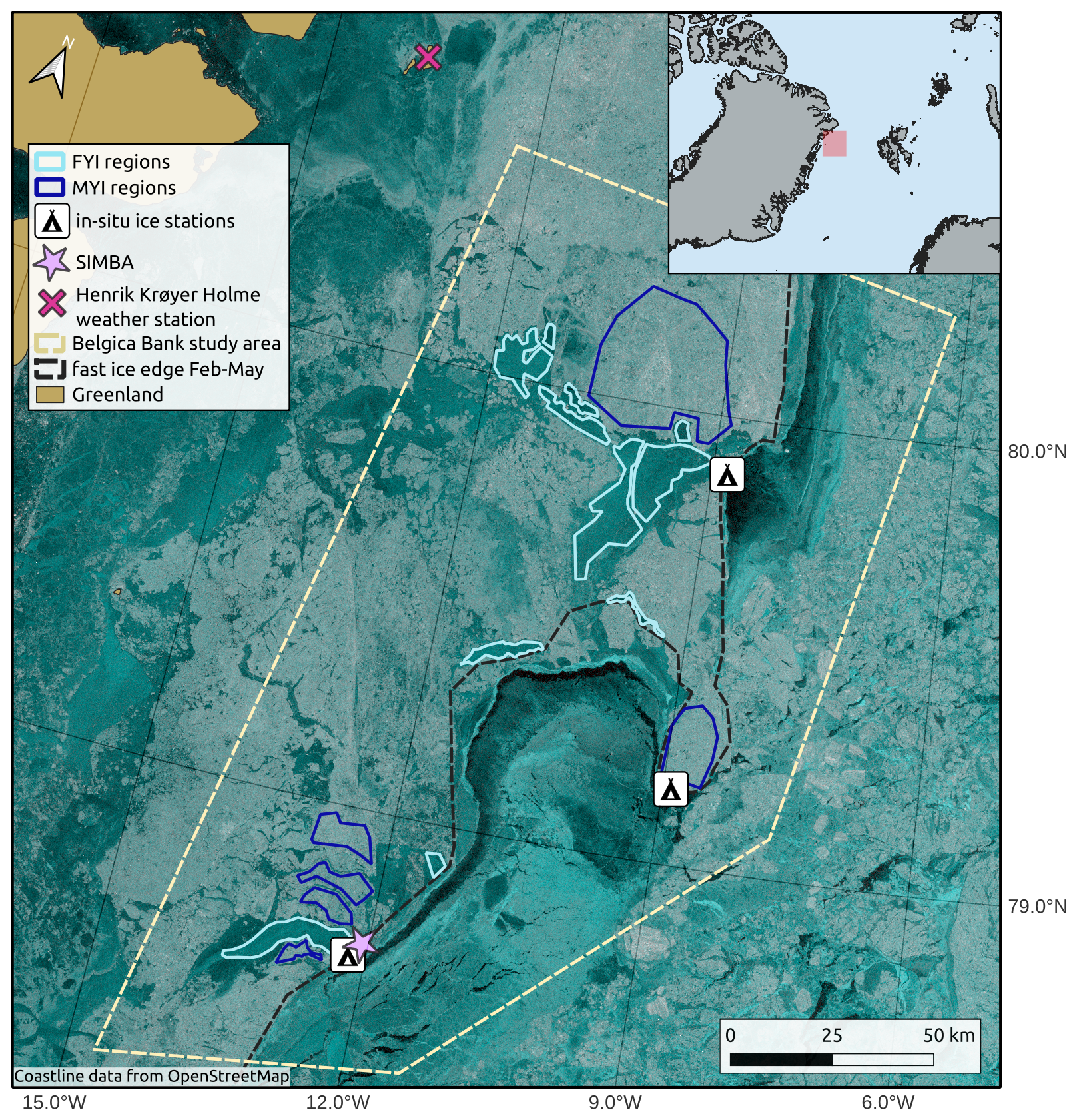
Figure 1 Overview map showing the FYI and MYI ROIs, in situ ice stations, and weather station in the Øer Ice Barrier area. The background is a Sentinel-1 false-color SAR image (HV-HH-HH) acquired on 28 April 2022 to illustrate the ice conditions at the time of the study. The fast ice edge outlined on the map shows the minimum fast ice extent for the months January–May 2022, hence it does not exactly match with the fast ice edge of the background SAR image (Coastline data from OpenStreetMap).

All ROIs selected for the FYI class form in situ in the Øer Ice Barrier within the span of 4 weeks in January–February 2022 and stay in place well into the melt season without experiencing significant deformation. This implies that all FYI ROIs undergo the full seasonal cycle which includes ice formation, snow accumulation and ice growth, and eventually melt or breakup. These ROIs thus capture the evolution from new ice to FYI. The class consisting of older, deformed ice generally contains areas with a mixture of heavily deformed MYI that is advected from further north and a smaller fraction of FYI that forms locally and is crushed in between the larger MYI floes. We refer to this as the MYI class in the remainder of this paper, as the ice in these areas predominantly has the characteristics of MYI and hence results are representative for Arctic MYI. For consistency, we choose to identify MYI ROIs that can be tracked throughout the same time period as the FYI. A total of 12 FYI and 6 MYI ROIs are outlined in this way, covering areas in the range 15–950 km², as shown in Fig. 1. All ROIs form or start being immobile between 25 January–22 February and break up between 15 May–8 August 2022.

3 Data

3.1 SAR

We gather a time series of C-band SAR imagery over the Øer Ice Barrier study area (outlined in Fig. 1) between October 2021 and August 2022. We use SAR images acquired by the Sentinel-1 (S-1) satellites from ESA, which image at C-band (5.405 GHz). All S-1 scenes used here are acquired in Extra Wide (EW) swath mode, which corresponds to a swath width of approximately 410 km. This mode images in dual-polarization (HH and HV) with incidence angles in the range 18.9–47°. The products are collected from the Copernicus Data Space Ecosystem in Ground Range Detected Medium resolution (GRDM) format, which has a spatial resolution of 93 m × 87 m (range-azimuth). The failure of Sentinel-1B in December 2021 led to a lower temporal resolution during the time of the study, but nevertheless there are on average two image acquisitions per day over the study area, resulting in a SAR time series of 366 images between January and August 2022.

3.2 Altimetry

After outlining the ROIs in the SAR imagery, we collect along-track laser and radar altimetry data that cover the Øer Ice Barrier study area between January and August 2022.

3.2.1 Laser altimetry

The Ice, Cloud, and land Elevation Satellite-2 (ICESat-2, hereafter referred to as IS-2) laser altimetry mission from NASA carries onboard the Advanced Topographic Laser Altimeter System (ATLAS). ATLAS is a photon-counting lidar operating at a 524 nm wavelength and providing surface height measurements across six different beams. The six beams are organized in pairs and one pair consists of a weak and a strong beam. The laser has a pulse repetition frequency of 10 kHz, which results in the ∼ 17 m (diameter) footprints being ∼ 0.7 m apart in along-track direction (Kwok et al., 2019). The satellite provides coverage up to 88° N.

We use the IS-2 ATL07 and ATL10 sea ice products. ATL07 contains along-track surface heights per track, provided in segments that corresponds to ∼ 150 photon aggregates. This means that the length of segments is not fixed but rather varies with surface type, i.e. a highly reflective surface will yield a shorter segment. As a result the ALT10 freeboard estimates come in varied along-track resolution (Kwok et al., 2021). The ATL10 product provides freeboard estimates per track, based on the ATL07 surface heights, where segments classified as sea surface provide reference sea surface tie points. Freeboard here means the total ice and snow freeboard. Note that the ATL10 product is only provided for areas with an ice concentration above 50 % and more than 25 km distance from land (Kwok et al., 2021), and that observations can be hindered by clouds. Furthermore, freeboard is only calculated when at least one sea surface reference point is available within 10 km distance along the same track. We use release 006 (r006) ATL07 and ATL10 data accessed through the National Snow and Ice Data Center (NSIDC) DAAC (Kwok et al., 2023).

3.2.2 Radar altimetry

We use radar altimetry data from the satellite missions CryoSat-2 (CS-2) and Sentinel-3 (S-3) A and B. The most recent Baseline 005 of the Sentinel-3 Sea Ice Thematic Product with the “Land” Processing Segment includes S-3 L1B pre-processed with the same configuration as CS-2 (Aublanc et al., 2025), so we use observations from the three sensors interchangeably. CS-2 carries a SAR Interferometric Radar Altimeter (SIRAL) operating at a Ku-band central frequency of 13.575 GHz. Over sea ice the device mainly operates in SAR mode. The Doppler processing in SAR mode results in higher along-track resolution of ∼ 350 m when compared to the conventional pulse-width limited altimetry, resulting in a footprint size of ∼ 350 m × 1600 m and coverage extends up to 88° N (ESA, 2026). The Sentinel-3A and -3B missions carry the SAR Radar ALtimeter (SRAL) sensor which operates at dual Ku/C-band frequency (13.575/5.41 GHz). The SAR processing at Ku-band produces a similar footprint size as CS-2 (Aublanc et al., 2025). The S-3 satellites only provide coverage up to 81.5° North, which is a benefit to this study because the Øer Ice Barrier lies around 80° N and is therefore well-covered near the orbital limit of S-3. Here, we use waveforms from the CS-2 level 2 baseline E SAR-mode product and S-3 level 2 baseline 005 product.

3.3 In situ measurements

The CIRFA-22 research cruise onboard RV Kronprins Haakon visited the Øer Ice Barrier in April–May 2022, providing a unique data set of snow and sea ice measurements in late Winter conditions. Snow and ice measurements were taken at three different locations on the fast ice, covering both level FYI and MYI, as shown in Fig. 1. The sampling locations were at a distance of 0–60 km away from the outlined ROIs and hence the in situ data is considered representative for the FYI and MYI in the ROIs. All measurements were obtained between 27 April and 3 May 2022, when air temperatures were in the range −20 to −7 °C. In the context of this study we use the following measurements: ice thickness from drill holes, snow properties from pits, snow and sea ice thickness data from collocated transects with a Magnaprobe (Sturm and Holmgren, 2018) and surface-based electromagnetic sounding (GEM-2 by Geophex Ltd., hereafter referred to as GEM) instrument, and vertical temperature profiles at 2 cm resolution in the snow and ice over the course of several weeks obtained from a Snow and Ice Mass Balance Apparatus (SIMBA) (Thompson et al., 2025). The Magnaprobe has a vertical sampling accuracy in the range 0–5 cm across all surfaces and horizontal positioning accuracy of ± 2.5 m (Sturm and Holmgren, 2018). The vertical accuracy of Magnaprobe measurements up to 5 cm is largely due to issues of “overprobing” when the substrate under the snow is soft (Sturm and Holmgren, 2018). Given the well defined nature of the snow/ice interface in the sea ice environment, we believe the accurary for our measurements is considerably lower than 5 cm. The GEM device has an accuracy of ± 0.1 m for the total thickness over level ice, but is significantly larger over deformed ice as it tends to underestimate the maximum depth of ridge keels. (Hunkeler et al., 2016; Haas and Jochmann, 2003).

A total of 10 snow pits were dug, spread over the three different ice stations and covering both FYI and MYI. The FYI snow pits were dug at the southern and northern ice stations, while the MYI snow pits were sampled at the middle station. The following physical snow properties were characterized layer-wise: density, grain size and type, and hardness. Temperature and salinity were measured at vertical resolutions of 5 and 3 cm, respectively. At every snow pit and at a few additional locations a bulk snow water equivalent (SWE) measurement was taken too. Ice cores were drilled at all three ice stations too and provide ice temperature, salinity, and density measurements. The latter were obtained through hydrostatic weighing. One collocated GEM and Magnaprobe transect is available over FYI, and another one over MYI. The SIMBA was deployed on MYI at the southern ice station and collected data from 28 April to 29 May 2022. The instrument recorded a vertical temperature profile every 6 h (including air temperatures just above the snow surface) and a heat conduction cycle every 24 h, from which snow depth and ice thickness was estimated. The reader is referred to the CIRFA-22 cruise report (Dierking et al., 2022) for detailed information about the in situ measurements.

The in situ data are inherently limited in quantity and spatial coverage, and only available for a short time span. These data are nonetheless valuable for a quantitative assessment of the satellite retrievals, as they are independent samples that are not susceptible to the same error sources and biases as the remote sensing observations. Furthermore, knowledge of in situ snow and ice properties helps to better constrain some of the free parameters in the satellite retrievals, such as snow and ice density in altimetry-derived ice thickness estimation.

3.4 Meteorological data

The SIMBA instrument provides in situ measurements of air temperature for the month of May only. We therefore also retrieve in situ daily averages of 2 m air temperature from the meteorological station Henrik Krøyer Holme (HKH) between 15 January and 5 August 2022. This station is located on an island near the Greenland coast, roughly 150 km north-west of our study sites and is operated by the Danish Meteorological Institute (DMI). The data is retrieved through the DMI Climate Data API (last accessed on 21 July 2025). In addition, air temperatures and daily total precipitation are retrieved from reanalysis over the same time period, providing estimates at larger scales and over the exact area of the study. We retrieve 2 m air temperatures at 12-hourly intervals and daily total precipitation over the Øer Ice Barrier from the Copernicus Arctic Regional ReAnalysis (CARRA) model (Schyberg et al., 2020), which comes at a 2.5 km horizontal resolution. Air temperatures from the HKH weather station were likely assimilated in CARRA. We determine the phase of the precipitation (rain or snow) at 3-hourly intervals using a linear approximation of the suit of exponential curves formulated in (Dai, 2008), with a center fraction of 0.5 at 1.1 °C.

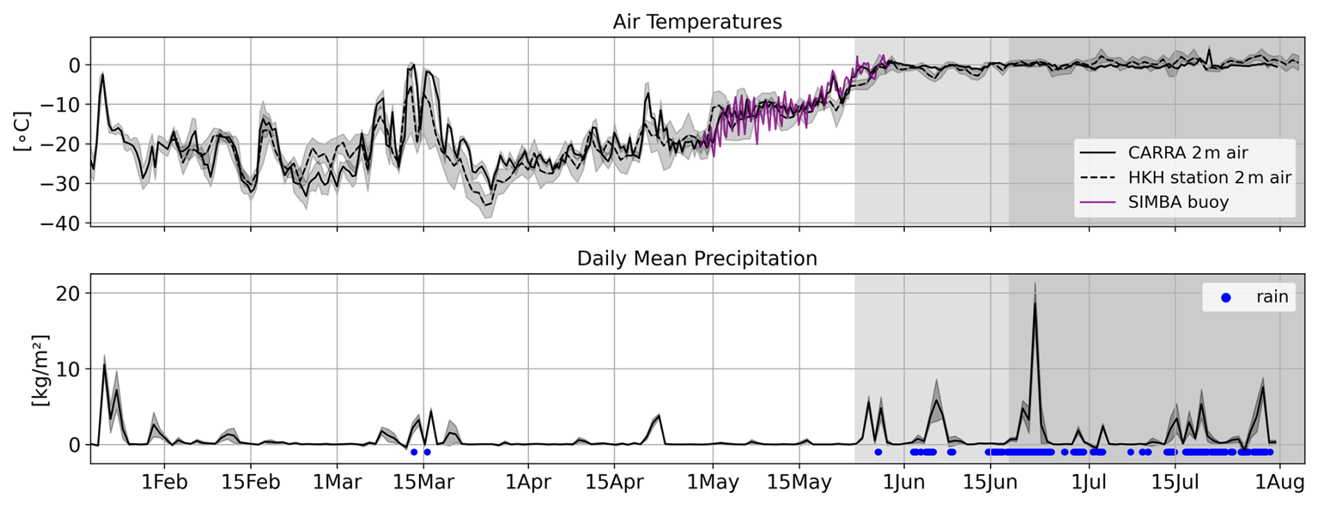
Figure 2 Air temperature and daily mean precipitation over the Øer Ice Barrier in Spring 2022. Air temperatures are shown for different data sources: CARRA reanalysis, Henrik Krøyer Holme (HKH) weather station, and SIMBA. Precipitation is only available from reanalysis (CARRA).

The time series of air temperature and precipitation is visualized in Fig. 2. As can be seen in this figure, the air temperatures of the different sources are in good agreement with each other. Spearman's correlation between CARRA and HKH 2 m air temperatures for the entire time of the study is 0.93 and the RMSE is 3.1 °C. The SIMBA air temperatures correlate more with air temperatures from CARRA than from HKH, with a correlation of 0.93 compared to 0.75, and RMSE of 1.6 versus 3.2 °C. The air temperatures modeled by CARRA thus seem to provide better estimates of local conditions over the study site, at least during the month of May, and we therefore use the CARRA air temperatures as reference in the remainder of this study. The figure also shows that before 1 June there are only three occasions where (part of the) precipitation fell as rain.

4 Methods

4.1 Definition of seasons

The time series covers both freezing and melting conditions. During the freezing conditions, a warming event occurs in mid-March with temperatures approaching zero degrees and strong snowfall lasting for ∼ 1 week. The transition period from freezing to melting conditions takes place in May–June. For this study, we define three seasons relevant from a remote sensing perspective, based on definitions that have been used in previous studies (Yackel et al., 2001; Karlsen et al., 2024): winter, melt onset, and advanced melt. The start of melt onset is defined as the first occurrence of a positive temperature in either the HKH station data, the CARRA reanalysis data, or the SIMBA data. Similarly, the transition from melt onset to advanced melt is defined as the latest date when temperatures are above zero degrees for at least 48 h consecutively in all three data sources. Using these definitions, melt onset starts on 24 May and advanced melt on 16 June 2022 (see Fig. 2). We provide a visual reference of these seasons in all time series plots by coloring the melt onset period in light gray and advanced melt in dark gray.

4.2 In situ measurements

The non-autonomous in situ measurements were taken between 27 April–3 May, which is in late winter but well before melt onset. The SIMBA instrument recorded data until 29 May, hence covering the transition from late winter to melt onset. We use the in situ measurements to obtain an average snow and ice density value per ice type, as well as distributions of snow and ice thickness per ice type. The average snow density is obtained by averaging the bulk SWE measurements per ice type. The bulk SWE values are preferred over averaging layer-wise densities from snow pits, since ice lenses and crusts in the snowpack are hard to sample with a density cutter and can therefore lead to underestimation of the snow density. The layer-wise measurements of snow temperature, salinity, and hardness are grouped across all snow pits per ice type and a median value is calculated in 10 % height intervals per property. For the ice density, one average value is calculated per ice type based on density measurements from the ice cores obtained by hydrostatic weighing. In situ snow and ice thickness distributions are inferred from the collocated GEM and Magnaprobe transects. Total snow plus ice thickness values are extracted from the GEM in-phase component at 18 330 Hz, following the approach described in (Itkin et al., 2023). The GEM device has a higher sampling frequency than the Magnaprobe, which has an irregular sampling frequency due to the manual handling. The Magnaprobe data is upsampled to the GEM sampling frequency by finding the spatially closest Magnaprobe sample for each GEM data point via a nearest neighbor search.

4.3 SAR

Pre-processing of the S-1 images includes denoising, radiometric calibration to σ₀, multi-looking the image with a window size of 3 × 3, conversion to decibels, and geocoding to polar stereographic projection (EPSG 3996) at a pixel spacing of 100 m. When investigating the radar backscatter evolution in a SAR time series that is not made up of repeat pass images, it is important to correct the backscatter values for variations in incidence angle (Yackel and Barber, 2000; Geldsetzer and Howell, 2023). This process is referred to as incidence angle normalization and implies finding a slope estimate and subsequently mapping all backscatter values to a common incidence angle using this slope estimate. Here, we estimate a slope from the SAR time series during the winter period using the differencing method presented in (Geldsetzer and Howell, 2023), where a slope estimate is calculated for each successive pair of SAR images where the same ice is imaged at two different incidence angles. The average slope value per ice type is then used to project the backscatter coefficients onto a common incidence angle of 35° for the entire SAR time series, including the melt season. See Appendix A1 for a detailed description of the incidence angle normalization procedure and slopes used here.

4.4 Radar Altimetry

4.4.1 Retracking

A radar altimetry waveform must be retracked to obtain an accurate measurement of the range between the altimeter and the surface. We retrack the CS-2 and S-3 waveforms using the LARM retracker, a physical-model retracker with a variable percentage threshold determined by the large-scale surface roughness and backscattering efficiency of the sea ice (Landy et al., 2020). Compared to retrackers with a fixed threshold, the variable threshold method can theoretically resolve thinner freeboards – down to a few centimeters – even over newly-formed ice with a very smooth surface, as well as thicker and rougher freeboards (Landy et al., 2020). In theory, the physical retracker is thus producing optimal height estimates, assuming there are no biases in the radar model or its assumptions. Here, we test this concept by applying the LARM retracker to retrieve a time series of radar freeboards over the same ice. Monitoring sea ice growth from its initial formation stage enables us to test the capability of the retracker to profile thinner and smoother ice, and to ascertain any systematic bias in altimetry-derived freeboard when ice thickness should be close to zero.

4.4.2 Waveform parameters

Different thresholds on varying waveform parameters exist to distinguish between echo returns from leads and sea ice, depending on the retracker algorithm used (Ricker et al., 2014). In this context, we retrieve the time series of the following commonly-used radar waveform parameters per ice type: sigma nought radar backscatter coefficients (σ₀), leading edge width (LEW) calculated for power thresholds of 5 % and 95 %, and pulse peakiness (PP) as formulated in (Ricker et al., 2014). The LEW mainly characterizes the influence of surface topography on the fitted waveform, while the PP is a measure of the specularity of the waveform (Wingham et al., 2006; Laxon, 1994). These waveform parameters are strongly correlated.

The σ₀ backscatter coefficients obtained with the S-3 sea ice retracker have not been calibrated against backscatter from CS-2 and therefore a significant offset in backscatter is observed between both sensors. We quantify the horizontal offset between the backscatter distributions from both sensors using the 1-D Wasserstein distance (Panaretos and Zemel, 2019) and find the offset to be 21 dB (See Sect. A3 in the Appendix). We then align the S-3 backscatter values to the CS-2 ones by subtracting 21 dB from the S-3 backscatter coefficients.

4.4.3 Removing lead tiepoints over fast ice

Visual comparison of spatio-temporally overlapping SAR and along-track radar freeboards revealed that many radar waveform returns over the FYI ROIs in both CS-2 and S-3 were wrongly classified as leads, even weeks after the ice had initially formed. See Sect. A2 in the Appendix for an example map showing the lead returns inside the FYI ROIs and generally inside the fast ice for the month of March. Over the newly-formed FYI areas, median LEW values are ∼ 0.5, PP in the range 50–100, and σ₀ backscatter in the range 20–30 dB. Typical thresholds for classifying a waveform as lead are LEW ≤ 0.75, PP ≥ 66, and σ₀ > 23 dB (Cryo-TEMPO and AWI products). The returns over newly-formed, smooth FYI often meet all three requirements and hence get misclassified. These observations are in line with the findings of Swiggs et al. (2025) showing an over-detection of leads from CS-2 in the Canadian Arctic Archipelago, in particular during the autumn freeze-up when there is a large fraction of thin ice (< 50 cm).

In the period February–May 1630 out of 55 670 S-3 returns and 811 out of 16 999 CS-2 returns are originally classified as lead over the fast ice inside the study area (i.e. the intersection between the Belgica Bank study area polygon and fast ice outline, see Fig. 1). It is important to note that some of these returns might indeed be leads. Here, we wish to focus on the impact of snow and sea ice radar scattering biases on retrieved freeboards in a controlled manner and wrongly classified returns could bias surrounding freeboard estimates. So, as this issue appears to be quite persistent in many of the ROIs in the time period after ice formation, we exclude all lead tie points within the fast ice between February–May, and re-process the CS-2 and S-3 freeboards using only lead tie points identified in the drift ice. This is achieved by applying a fast ice mask (see Fig. 1) before identifying lead tie points to calculate freeboard values. The impact of the masking on the radar freeboard time series is as follows: the Root Mean Squared Error (RMSE) is 0.0065 m over FYI and 0.0049 m over MYI. The masking effect is larger over the FYI ROIs, as these are the regions that contain many returns classified as lead in the original data product, while for MYI the returns are classified correctly as ice but subsequent freeboard calculations are affected if false lead tie points are used to obtain sea surface height anomaly estimates. We assume the impact is small because the fast ice areas classified as lead are typically very thin, newly-formed ice areas with a freeboard close to sea level. More details are provided in Sect. A2 in the Appendix.

4.5 Laser Altimetry

4.5.1 Custom interpolation scheme for freeboard derivation in lead-sparse areas

The IceSat-2 ATL10 freeboard product as provided by NSIDC does not contain freeboard values for samples where the closest lead tie point is more than 10 km away (Kwok et al., 2023). Since the ROIs in this study are located in an area of immobile landfast ice at distances between 0–65 km away from the fast ice edge, the standard 10 km limit provides no ATL10 freeboard data over a large part of our study – even in locations where a valid ATL07 surface height had been obtained. Adding to this problem is the fact that lead tie points cannot be used across the six IS-2 beams when calculating sea surface height anomaly (SSHA) estimates, because the different beams have not yet been calibrated against each other and centimeter-scale deviations in range remain (Bagnardi et al., 2021). While the NSIDC ATL10 product uses a strict 10 km limit to ensure high data quality for downstream monthly aggregates where data density is high, our objective requires maximizing spatial and temporal coverage over the ROIs. We therefore implement a custom freeboard derivation where the closest lead tie point can be up to 100 km away. For each ATL07 surface height sample the ten closest lead tie points along the same beam are identified with a k-nearest neighbor search. An interpolated SSHA is then calculated for each ATL07 sample where no ATL10 freeboard is available, using an inverse distance squared weighted (IDW) interpolation of the SSHA of the 10 nearest neighbours, as given by Eq. (1).

$$\begin{array}{}\text{(1)}& \text{SSHA}[i{]}_{\text{interpolated}}={\displaystyle \frac{{\sum }_{k=\mathrm{1}}^{\mathrm{10}}\left({\text{SSHA}}_k\cdot \frac{\mathrm{1}}{D_k^{\mathrm{2}}}\right)}{{\sum }_k\frac{\mathrm{1}}{D_k^{\mathrm{2}}}}}\end{array}$$

Here k is the kth nearest lead tie point of sample i in the ATL07 heights and D the distance from this sample to the lead tie point. The freeboard value then equals the ATL07 height minus the interpolated SSHA, as given by Eq. (2). Samples that have an original ATL10 freeboard value are kept as such.

$$\begin{array}{}\text{(2)}& \mathrm{FB}\left[i\right]=\left\{\begin{array}{ll}\begin{array}{l}\text{h}[i{]}_{\text{ATL07}}\\ -\text{SSHA}[i{]}_{\text{interpolated}}\end{array}& \text{if }\mathrm{FB}[i{]}_{\text{ATL10}}=\text{NaN}\\ \mathrm{FB}[i{]}_{\text{ATL10}}& \text{otherwise}\end{array}\right.\end{array}$$

We acknowledge that the IDW interpolation method is relatively simplistic and may not fully capture the complex ice dynamics typical of near-shore environments. However, implementing a more complex interpolation scheme without rigorous, independent validation could introduce greater uncertainties and artifacts than this straightforward IDW approach. We validate the interpolation scheme and determine the optimal search distance for lead tie points through a sensitivity analysis that compares independent laser altimeter overpasses intersecting over the fast ice within a set time window. The analysis compares the mean laser freeboard from pairs of intersecting beams within radii of 250, 500, and 1000 m and within a time interval of at most 10 d (≃ 240 h), using maximum search distances of 50, 80, 100, and 150 km for the lead tie points. More details about the sensitivity analysis are provided in Sect. A4 in the Appendix. The analysis shows that (i) data density increases when increasing the maximal search distance for lead tie points, and (ii) laser freeboards generally show good agreement between overpasses, with correlation coefficients in the range 79–86 for intersections with a time lag of 34 h. Some variability is expected due to the nature of the experiment, as we do not look at exact repeat passes, but rather at intersections where track A does not sample the exact same ice surface as track B. The correlation coefficients across the different time lags are stable or even slightly improve for maximal lead tie points distances up to 100 km, but start decreasing for 150 km distance. We conclude that the IDW method with 100 km distance threshold provides reliable sea surface height estimates while maximizing laser altimetry coverage, and use this method to obtain a laser freeboard for each ATL07 height sample without corresponding ATL10 freeboard. Figure 3 shows the laser freeboards for pairs of intersecting beams within a radius of 1000 m, using 100 km as maximum distance for detecting lead tie points. The figure is color-coded by time lag and reports the corresponding Spearman correlation coefficients (R).

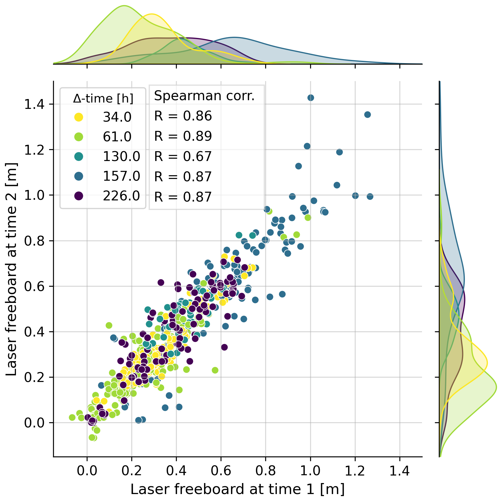
Figure 3 Comparison of mean laser freeboards for pairs of intersecting IS-2 beams, color-coded by time lag. Spearman's correlation coefficient (R) is reported per time lag and kernel density estimated PDF's are shown on the sides.

4.6 Laser and radar freeboard time series construction

This section describes how data from the individual ROIs is combined to obtain one laser freeboard and one radar freeboard time series per ice type. We explain the steps taken to mitigate representation issues, random errors inherent to the altimetry sampling process, and the systematic bias that could arise due to the discrepancy in footprint size of the laser and radar altimeters.

The different, non-contiguous ice surfaces within ROIs of the same ice type have a similar radar backscatter intensity and texture appearance in the SAR images. Moreover, all FYI regions form within a span of 4 weeks and mature similarly since the ice is immobile and therefore only grows thermodynamically. We therefore consider the different ROIs of one ice type as subsets sampling the same ice, i.e. we consider them as one large ROI. This implies that the along-track freeboards from an altimetry track crossing any of the ROIs is a representative sample for the corresponding ice type. With this reasoning in mind, all altimetry tracks from IS-2, CS-2, and S-3 that intersect with any of the ROIs in the time frame of the study are gathered per ice type, with the benefit of finer temporal sampling of the time series. For each intersection we calculate the median and inter-quartile range (IQR) of the along-track freeboards that are within the ROI boundaries. The ROI diameters are in the range 1–38 km, so freeboards are averaged along segments within this range. This spatial averaging is desired as along-track laser and radar freeboards contain random errors due, for example, to speckle noise and uncertainties in the sea surface height interpolation (Wingham et al., 2006; Ricker et al., 2014). For the laser freeboards we take the median of all six IS-2 beams together in order to minimize representation issues due to the sampling of varying snow and/or ice distributions. This step further increases the spatial averaging as the IS-2 beam pairs are ∼ 90 m apart and pairs are separated ∼ 3 km across track. Freeboard is a relative measure and therefore inter-beam range biases cancel out. Using the median instead of the mean per crossing prevents topographic features resolved by the finer laser footprint, but potentially missed by the larger radar footprint (e.g. ridges), influencing the freeboard value that feeds into the time series. This minimizes any potential systematic bias that could arise from the footprint size discrepancies between the laser (∼ 17 m) and radar (∼ 300 m) sensors. The result after this first processing step is a time series of laser and radar freeboards per ice type that is composed of the median freeboard value (plus IQR) per altimeter crossing.

For FYI the time series is constructed in a relative way too, meaning that timestamp t=0 is the ice formation date. This is achieved by referencing every freeboard sample to the formation date of the ROI this sample originates from. The result is a relative time series that visualizes the seasonal evolution of FYI, which includes the initial ice formation, snow accumulation and ice growth, and subsequent melt. The relative time series captures the evolution of altimetry signatures from newly-formed ice to snow-covered FYI more accurately by accounting for the differences in ice evolution between ROIs in the first few weeks after ice formation. The drawback with the relative approach is that it is not possible to directly link the time series to atmospheric conditions. We set 8 February as t=0 in the plots for the relative FYI time series, which corresponds to the average FYI ice formation date. The MYI time series is only constructed in absolute time, as here the ice is already matured and snow-covered when we start monitoring it and hence no significant changes are expected at short time scales. The MYI time series is meant to serve as a reference in the interpretation of the FYI time series.

In a second step, we interpolate the freeboard time series composed of the original median freeboards from crossings to daily resolution. The time series of radar freeboards are more dense than the laser ones, as there are three radar altimeters and only one laser altimeter. This effect is amplified by S-3A and B having a much higher temporal resolution and spatial coverage over the Øer Ice Barrier compared to CS-2 and IS-2. Sampling onto a regular temporal grid is necessary to calculate dual-frequency snow depths, and subsequently SIT. We interpolate the laser and radar freeboard time series to daily temporal resolution using a Radial Basis Function interpolator with a Gaussian kernel with standard deviation of 11.8 d. This kernel effectively acts as a temporal low-pass filter and thus reduces the latent representation errors that affect the median freeboards derived from individual altimeter crossings. The interpolation is most likely over-generalizing the true temporal variability in freeboards, as changes in freeboard height related to synoptic weather systems that fall below the kernel size are either entirely smoothed away, or at least underestimated in the interpolated time series. This is more impactful for the laser freeboard time series, with sparser data coverage, than the relatively dense radar freeboard time series. Nevertheless, an interpolation that over-generalizes is preferred over one that under-generalizes, as we need to ensure that interpreted patterns in the time series are not originating from the variability that is inherent in the altimetry sampling (owing to noise and representation error).

The two-step spatio-temporal averaging procedure reduces the random uncertainties inherent to the along-track altimetry sampling and mitigates representation errors. We therefore expect that fluctuations in the interpolated laser or radar time series mostly represent physical changes in the snow and ice cover. These physical changes may characterize actual variations in the dominant radar scattering processes in the snow and ice, or the effects of e.g. physical changes in snow on the retracker (that assumes ice surface scattering to be the dominant return). Nevertheless, representation issues might to some degree still persist, particularly in the MYI laser freeboard time series. Due to its rough surface topography and longer period of snow accumulation, the snow distribution on MYI is highly heterogeneous. Furthermore, laser altimetry coverage is lower over the MYI ROIs compared to the FYI ones. While the grouping of all six IS-2 beams and the subsequent interpolation reduces representation artifacts, they cannot be entirely eliminated and therefore fluctuations in the MYI laser freeboard time series should be interpreted with caution. Following all these processing steps, we believe the differences between the interpolated laser and radar freeboard time series mainly reflect differences in the wavelength-dependent interaction of the electromagnetic waves with the snow and ice cover.

4.7 Freeboard-to-thickness conversion

Under the assumption of isostatic equilibrium, ice freeboard (FB_i) can be converted to ice thickness (SIT) using Eq. (3), provided that the snow depth (SD) and densities of snow (ρ_s), sea ice (ρ_i), and sea water (ρ_w) are known (Laxon et al., 2003). This section outlines how we determine values for snow and ice densities, and how we estimate snow depth.

$$\begin{array}{}\text{(3)}& \text{SIT}({\mathrm{FB}}_{\mathrm{i}},\text{SD})={\displaystyle \frac{{\mathit{\rho }}_{\mathrm{w}}}{{\mathit{\rho }}_{\mathrm{w}}-{\mathit{\rho }}_{\mathrm{i}}}}{\mathrm{FB}}_{\mathrm{i}}+{\displaystyle \frac{{\mathit{\rho }}_{\mathrm{s}}}{{\mathit{\rho }}_{\mathrm{w}}-{\mathit{\rho }}_{\mathrm{i}}}}\text{SD}\end{array}$$

4.7.1 Density of snow, sea ice, and sea water

Snow – Choosing an appropriate bulk snow density is challenging because the density of snow can be highly variable at short spatiotemporal scales – both in the vertical and horizontal direction. Snow densities in this study are based on the in situ values from the ten snow pits dug in late April during the CIRFA-22 cruise. Snow on sea ice tends to densify throughout the season (Barber et al., 1995). We therefore implement a linear time-dependent equation for snow density, using the seasonal densification rate identified in (Mallett, 2025) and calibrate the offset to match the in situ snow density measurements of late April, which are: 298 ± 81 kg m⁻³ for FYI and 302 ± 66 kg m⁻³ for MYI. This results in Eq. (4) for FYI and Eq. (5) for MYI, where T_a is the number of days since ice formation for FYI, and the number of days since 1 August for MYI. For FYI we calculate T_a relative to the average ice formation date of all FYI ROIs, which is 8 February 2022. This is deemed reasonable since all FYI ROIs form within 2 weeks from this date.

$$\begin{array}{}\text{(4)}& {\displaystyle }{\mathit{\rho }}_{\text{FYI}}=\mathrm{0.35}{T}_{\mathrm{a}}+\mathrm{270}\text{(5)}& {\displaystyle }{\mathit{\rho }}_{\text{MYI}}=\mathrm{0.35}{T}_{\mathrm{a}}+\mathrm{207}\end{array}$$

Sea ice – For ice density (ρ_i), common approaches include an ice type-dependent definition of density based on field measurements from the 1980's, or using a single ice density (Kacimi and Kwok, 2024). The single value approach might arguably better represent the ice density in the current Arctic, as more recent studies indicate that MYI densities appear to be closer to the FYI ones, especially for younger MYI (Jutila et al., 2022; Shi et al., 2023). Commonly used values are 917 kg m⁻³ for FYI and 882 kg m⁻³ for MYI, or 915–917 kg m⁻³ when using a single value (Kacimi and Kwok, 2024). In reality, ice density varies throughout the season and additionally depends on ice type, age, temperature, and thickness (Salganik et al., 2025). Jutila et al. (2022) found a negative exponential relationship between Arctic spring sea ice freeboard and density. However, at present there is no conclusive parametrization for the temporal evolution of sea ice density over the course of a winter season. We therefore consider the in situ ice density values obtained from ice cores taken at the end of April as the best estimates of ice density in our ROIs and use these values for the entire time series. The average value for FYI obtained from the cores is 914 ± 2 kg m⁻³, while for MYI it is 909 ± 3 kg m⁻³.

Sea water – For near-surface sea water (ρ_w) we use the conventional density of 1024 kg m⁻³ (Wadhams et al., 1992).

4.7.2 Snow depth from laser and Ku-band radar freeboards (“LaKu”)

Snow depth estimates can be obtained from near-coincident laser and radar freeboard observations (Kwok et al., 2020; Fredensborg Hansen et al., 2024; Carret et al., 2025). Dual-altimetry snow depth is derived by differencing the laser freeboard (FB_La) from the ice freeboard (FB_i):

$$\begin{array}{}\text{(6)}& \text{SD}={\mathrm{FB}}_{\mathrm{La}}-{\mathrm{FB}}_{\mathrm{i}}\end{array}$$

The ice freeboard can be obtained from the radar freeboard (FB_Ku) by accounting for the slower propagation speed of radar waves in snow (c_s) compared to free space (c) (Ulaby et al., 1981). The refractive index for snow (n_s) is dependent on the snow density (ρ_s) as given by Eq. (7) (Ulaby et al., 1981) and is used to convert FB_Ku to FB_i using Eq. (8).

$$\begin{array}{}\text{(7)}& {\displaystyle }& {\displaystyle }{n}_{\mathrm{s}}={\displaystyle \frac{c}{c_{\mathrm{s}}}}=(\mathrm{1}+\mathrm{0.00051}{\mathit{\rho }}_{\mathrm{s}}{)}^{\mathrm{1.5}}\text{(8)}& {\displaystyle }& {\displaystyle }{\mathrm{FB}}_{\mathrm{i}}={\mathrm{FB}}_{\mathrm{Ku}}+\text{SD}(n_{\mathrm{s}}-\mathrm{1})\end{array}$$

By substituting Eq. (8) into Eq. (6) and solving for SD, the following expression for snow depth is obtained:

$$\begin{array}{}\text{(9)}& \text{SD}={\displaystyle \frac{{\mathrm{FB}}_{\mathrm{La}}-{\mathrm{FB}}_{\mathrm{Ku}}}{n_{\mathrm{s}}}}\end{array}$$

Note that this expression is dependent on snow density through the refractive index n_s. Equation (9) is used here to calculate a daily SD estimate from the interpolated laser and radar freeboard time series, using the time-dependent snow densities as defined in Eqs. (4) and (5) for FYI and MYI, respectively.

Previous studies reported relatively high uncertainties for along-track LaKu snow depth retrieval (Fredensborg Hansen et al., 2024; Saha et al., 2025). In Fredensborg Hansen et al. (2024) the authors find an average uncertainty along 7 km segments of 10–11 cm, composed of random and systematic contributions of 7 and 4 cm. When calculating LaKu from monthly gridded products at 25 km resolution, the average uncertainty is reduced to 6 cm (Carret et al., 2025). Here, we are not able to reliably assess the average uncertainty for the freeboard time series. However, with the two-step spatio-temporal averaging procedure used to construct the laser and radar freeboard time series, we expect the random uncertainty in our LaKu snow depth time series to be lower compared to the values reported for along-track LaKu snow depth, but likely higher than the monthly gridded products. The systematic uncertainty can originate from different sources, such as choices in the retracking methodology or uncertain Ku-band radar penetration into the snow, and is therefore difficult to estimate (Fredensborg Hansen et al., 2024). Since we do not have a good estimate of the average uncertainty, we visualize the spread (IQR) in the freeboard retrievals and subsequent snow depth and ice thickness estimates.

4.7.3 Ice thickness from radar freeboard

The freeboard-to-thickness conversion outlined in Eq. (3) requires FB_i as input. Radar freeboards are linked to ice freeboards via Eq. (8), so by plugging Eq. (8) into Eq. (3), an expression for ice thickness as function of radar freeboard is obtained:

$$\begin{array}{}\text{(10)}& \begin{array}{rl}{H}_{\mathrm{i}}({\mathrm{FB}}_{\mathrm{Ku}},\text{SD})=& {\displaystyle \frac{{\mathit{\rho }}_{\mathrm{w}}}{{\mathit{\rho }}_{\mathrm{w}}-{\mathit{\rho }}_{\mathrm{i}}}}{\mathrm{FB}}_{\mathrm{Ku}}\\ & +{\displaystyle \frac{{\mathit{\rho }}_{\mathrm{w}}(\mathrm{1}+\mathrm{00051}{\mathit{\rho }}_{\mathrm{s}}{)}^{\mathrm{1.5}}-{\mathit{\rho }}_{\mathrm{w}}+{\mathit{\rho }}_{\mathrm{s}}}{{\mathit{\rho }}_{\mathrm{w}}-{\mathit{\rho }}_{\mathrm{i}}}}\text{SD}\end{array}\end{array}$$

The dual-altimetry snow depths and densities outlined above are used in this equation to convert the radar freeboard time series into an ice thickness time series per ice type.

4.8 Modeled snow accumulation and ice growth

To provide context for the snow depth and ice thickness time series obtained from the altimetry observations and support its interpretation, we model snow accumulation and thermodynamic ice growth at the FYI and MYI sites during the period of the study. Since the ice is immobile, we can assume the ice did not thicken dynamically through ridging, so that total ice growth is exclusively thermodynamic. We use a combination of SnowModel and HIGHTSI as decribed in Itkin and Liston (2025). The model is initialized with 0.3 m sea ice thickness on 10 October 2021 for MYI and by zero ice thickness on 8 February 2022 for FYI, which corresponds to the average formation date of the FYI regions. Afterwards, the model is forced with the air temperature and precipitation data from CARRA (see Sect. 3.4). The surface ocean heat fluxes and other variables do not have a significant impact on the simulation results and are set as in Itkin and Liston (2025). The snow depths and densities from in situ observations (Sect. 3.3) are assimilated to correct the bias in precipitation, and the sea ice thickness is simulated based on these adjusted snow properties. The main focus is the modeled ice growth and snow accumulation of FYI, since this is well-constrained and as such provides a good reference for the altimetry-derived LaKu snow depth and SIT.

4.9 Modeled dielectric properties of snow on sea ice

4.9.1 Complex dielectric constant of snow

The presence of salt in snow impacts radar wave propagation because it introduces liquid water in the snow at temperatures below 0 °C. The liquid water alters the complex dielectric constant of the snow, leading to increased absorption (Ulaby et al., 1981; Barber and Fung, 1998; Geldsetzer et al., 2009). Here, we investigate the impact of saline snow on Ku-band wave propagation by modeling the complex dielectric constant in fresh (i.e. MYI) versus saline (i.e. FYI) snow at Ku-band frequency. The salt content is typically highest at the base of the snow pack, so we model the complex dielectric for the basal layer only as this will highlight the differences between saline and fresh snow. We define the basal layer as the bottom 10 % of the snow pack height. In this study, the average height of the basal layer is 2 cm for FYI and 3.5 cm for MYI. The complex dielectric constant of the snow (ε_s) is estimated using the frequency dispersion model of Geldsetzer et al. (2009) as formulated in Eq. (11), which allows for either fresh or saline snow.

$$\begin{array}{}\text{(11)}& \begin{array}{rl}& {\mathit{\epsilon }}_{\mathrm{s}}={\mathit{\epsilon }}_{\mathrm{s}}^{\prime }-i{\mathit{\epsilon }}_{\mathrm{s}}^{\prime \prime }\text{ where }{\mathit{\epsilon }}_{\mathrm{s}}^{\prime }={\mathit{\epsilon }}_{\text{ds}}^{\prime }+S\mathit{\phi }{\mathit{\epsilon }}_{\mathrm{b}}^{\prime }\text{ and }\\ & {\mathit{\epsilon }}_{\mathrm{s}}^{\prime \prime }={\mathit{\epsilon }}_{\text{ds}}^{\prime \prime }+S\mathit{\phi }{\mathit{\epsilon }}_{\mathrm{b}\left(\text{rel}\right)}^{\prime \prime }+{\mathit{\epsilon }}_{\mathrm{s}\left(\text{cond}\right)}^{\prime \prime }\end{array}\end{array}$$

With ε_s, ε_ds, and ε_b the complex dielectric constants of snow, dry snow and brine, respectively, S the depolarization factor, φ the brine volume fraction. The contributions from relaxation (rel) and conductivity (cond) to ${\mathit{\epsilon }}_{\mathrm{b}}^{\prime \prime }$ are treated separately (Geldsetzer et al., 2009). Estimating the input parameters requires knowledge about the snow temperature, density, salinity, and crystal size. We quantify these variables from the in situ data, using the measurements obtained in the bottom 10 % of the studied snow packs. We use snow temperatures measured by the SIMBA instrument in the snow layer 0–4 cm above the snow/ice interface, available from late April until the end of May. This covers the time period leading up to melt onset, where temperatures gradually rise from ∼ −20 to 0 °C. The frequency dispersion model is valid for snow temperatures below −3 °C, so we limit the modeling to this temperature range. We do not have SIMBA data over FYI, so we use the MYI basal snow temperatures for the FYI simulations too. For the snow salinity, density, and crystal size, we use median values from the bottom 10 % of the snow pits, per ice type. These snow properties were observed in late April and are used here to model the snow throughout the month of May due to the lack of repeat measurements. We expect, however, that the first-order mechanisms responsible for changes in the dielectric snow properties at microwave frequencies are still modeled correctly through the coupled temperature-salinity effects, assuming that the snow did not significantly desalinate over the course of these 4 weeks.

4.9.2 Radar penetration depth

Changes in the dielectric properties of the snow impact the characteristic distance an electromagnetic wave can penetrate into the snow layer. The penetration depth is defined as the depth into a medium at which the power of the wave is reduced to a factor e⁻¹ the power of the incident wave at the upper surface of the medium (Ulaby et al., 1981). We model the radar penetration depth into the basal snow layer, i.e. the bottom 10 % of the snow pack, at Ku-band frequency for the time period in situ snow temperatures are available from the SIMBA instrument. The modeled penetration depth gives a theoretical lower bound on the depth inside the basal snow layer from where significant radar energy is expected to return to the sensor, assuming an idealized snow layer where surface scattering at the air/snow interface is minimal. Note that this single-layer model does not take into account the presence of ice underneath the snow and hence does not include surface scattering at the snow/ice interface. The goal here is to model how the presence or absence of salt in the basal snow layer affects the Ku-band radar penetration depth inside this snow layer. The radar penetration depth (δ_p) is modeled as:

$$\begin{array}{}\text{(12)}& {\mathit{\delta }}_{\mathrm{p}}={\displaystyle \frac{\mathit{\lambda }}{\mathrm{4}\mathit{\pi }}}{\left\{\left[{\left(\mathrm{1}+{\left({\displaystyle \frac{{\mathit{\epsilon }}^{\prime \prime }}{{\mathit{\epsilon }}^{\prime }}}\right)}^{\mathrm{2}}\right)}^{\mathrm{1}/\mathrm{2}}-\mathrm{1}\right]{\displaystyle \frac{{\mathit{\epsilon }}^{\prime }}{\mathrm{2}}}\right\}}^{-\mathrm{1}/\mathrm{2}}\cdot \text{cos}\left({\mathit{\theta }}_i\right)\end{array}$$

where λ is the wavelength, ε^′ and ε^′′ are real and imaginary part of the complex dielectric constant of the basal snow layer, and cos(θ_i) the incidence angle of the EM-wave (Ulaby et al., 1981). The complex dielectric constant of the snow is estimated through Eq. (11), for saline (FYI) and fresh (MYI) snow. For nadir-looking sensors, such as the radar altimeters CS-2 and S-3, the incidence angle is set to zero.

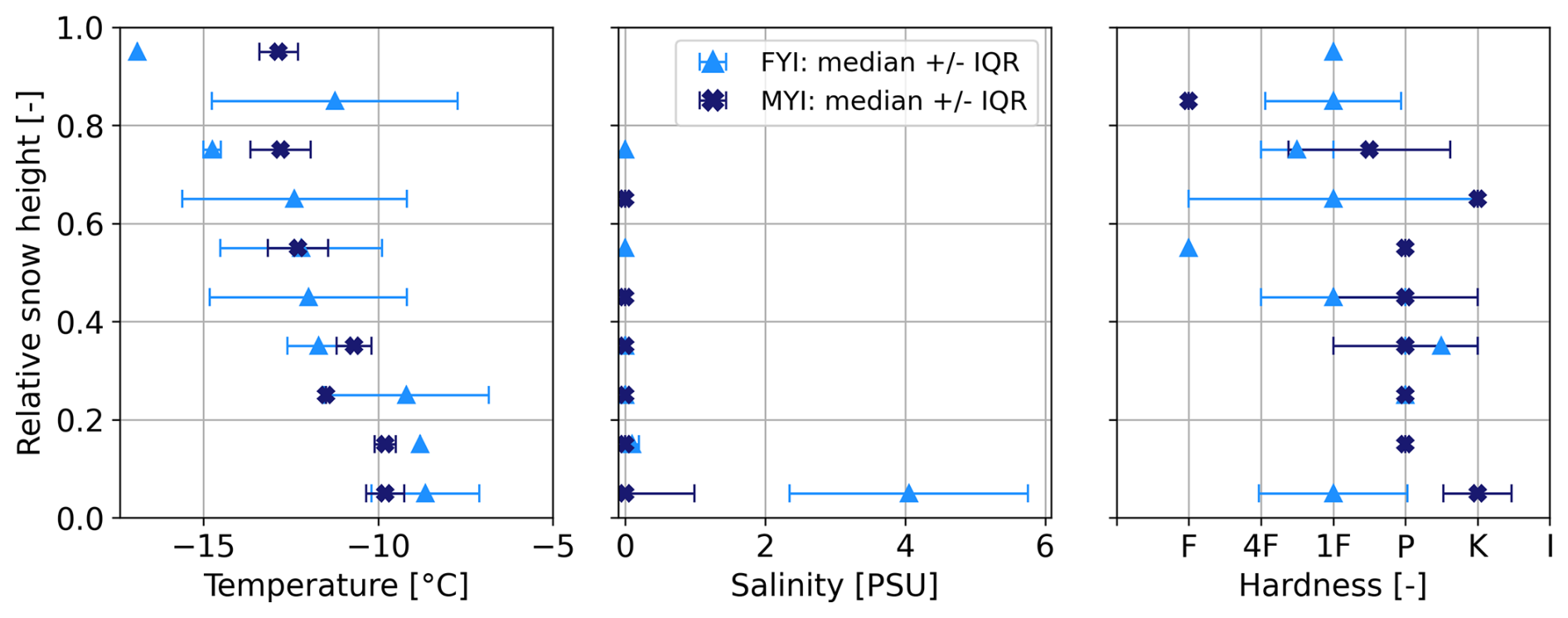
Figure 4 In situ snow properties averaged across all snow pits in 10 % height intervals: temperature, salinity, and hardness. The hardness letter codes are: fist (F), 4 fingers (4F), 1 finger (1F), pencil (P), knife (K), ice (I) (Fierz et al., 2009). Profiles are shown in relative snow height, with 0 the bottom and 1 the top of the snow pit.

5 Results

5.1 In situ snow and ice properties

Ten snow pits were physically sampled in the study area between 27 April–3 May 2022, seven on FYI and three on MYI (see Fig. 1 for locations). The FYI snow pit heights were in the range 10–35 cm (mean 20 cm), while MYI snow pit heights were 18–28 cm (mean 24 cm). All studied snow packs show typical characteristics of snow on Arctic sea ice in late Winter. Every snow pit was characterized by a soft, low-density basal layer composed predominantly of depth hoar crystals with diameters in the range 0.5–6 mm (FYI) and 0.5–11 mm (MYI). For all FYI pits this bottom layer was saline, with salinity values between 3–6 PSU and a mean of 4.2 PSU. Saline snow was found up to 6 cm away from the snow/ice interface, albeit at lower salinity values higher up in the snow pack (salinity < 1 PSU at 6 cm). The upper layers of the pits were more varied, but generally had a higher density and smaller crystals, often faceted or rounded, which is characteristic for Arctic snow packs (Sturm et al., 1827). Some pits had ice lenses and crusts that were potentially formed during the warming event in March. Figure 4 shows the median snow temperature, salinity, and hardness in 10 % height intervals across all snow pits. The average snow density obtained from bulk SWE measurements was: 298 ± 81 kg m⁻³ for FYI and 302 ± 66 kg m⁻³ for MYI. Regarding ice density, the average value for FYI obtained from the cores was 914 ± 2 kg m⁻³, while for MYI it was 909 ± 3 kg m⁻³.

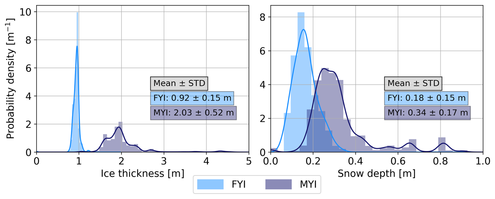
Figure 5 Ice and snow thickness distributions from collocated GEM and Magnaprobe transects over FYI and MYI in the Øer Ice Barrier at the end of April. The mean and standard deviation of the snow depth and ice thickness are obtained by averaging the data of all transects per ice type.

Snow depth and ice thickness distributions from collocated GEM and Magnaprobe transects are visualized in Fig. 5. Over FYI the ice was 0.92 ± 0.15 m with a snow cover of 0.18 ± 0.15 m, while over MYI the ice was 2.03 ± 0.52 m with 0.34 ± 0.17 m snow.

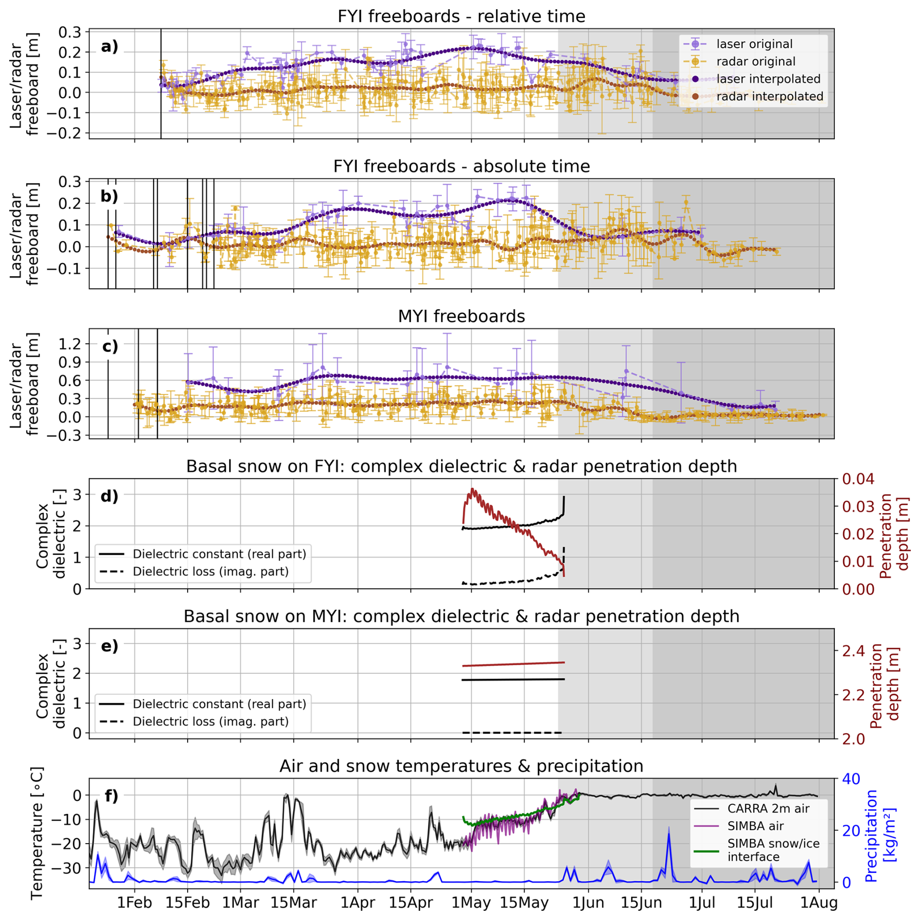
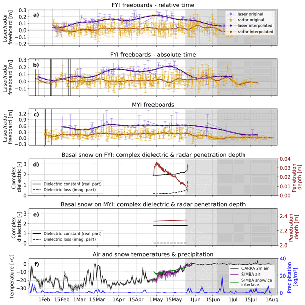
Figure 6 Panels (a–c): time series of laser and radar freeboards over FYI (relative and absolute time) and MYI, respectively, showing original samples (median + IQR) as well as daily interpolated values. The FYI time series in relative time is obtained by aligning the data points of individual FYI ROIs such that timestamp t=0 corresponds to the moment of ice formation. The relative timestamp t=0 is mapped to 8 February in this figure, which corresponds to the average date when the FYI ROIs form. The MYI time series is only produced in absolute time. Black vertical lines mark the timestamps when we start tracking individual ROIs. Note the difference in scales between the y-axes of FYI and MYI plots. Panels (d, e): modeled complex dielectric constant and radar penetration depth for basal snow on FYI and MYI, respectively. Panel (f): atmospheric conditions. The background colors highlight the different seasons: winter–melt onset–advanced melt.

5.2 Temporal evolution of laser and radar freeboards

Figure 6a–c show the time series of radar and laser freeboards for FYI (relative and absolute time) and MYI, respectively. The original data points are shown with light-colored markers (median) and error bars representing the spread (IQR). The daily interpolated values are visualized dark-colored markers. Black vertical lines indicate the timestamps at which we start tracking different individual ROIs. Note it is radar freeboards that are shown here, so no correction for slower wave propagation in snow is applied.

For FYI, the moment of ice formation is best captured in the relative time series (Fig. 6a), while changes due to atmospheric conditions, such as the warming event or melt onset, are best analyzed from the absolute time series (Fig. 6b). The moment of ice formation is marked by relatively high radar freeboards (∼ 0.07 m), while laser freeboards are lower (∼ 0.04 m) but still largely above zero. Within a week after ice formation the laser freeboards start rising, while radar freeboards initially drop to values just below zero and only start rising approximately 2 weeks after ice formation. In both the relative and absolute time series, the laser freeboards rise at an average rate of 0.25 cm d⁻¹, representing snow accumulation and sea ice growth, until reaching a maximum around 0.22 m in the middle of May. Radar freeboards show a slight positive trend of 0.06 cm d⁻¹ in the same time period. Laser freeboards tend to increase stepwise, following the precipitation events, while the radar freeboards show a more linear increase throughout the winter period. Note that the sudden jumps in laser freeboards following precipitation events are smoothed out in the interpolated time series and appear less pronounced. The absolute time series shows that the radar freeboards exhibit a temporary (∼ 7–10 d) rise of ∼ 4 cm around 15 March, coinciding with the warming event that includes heavy snowfall. An opposite dynamic is observed around 10 May, when radar freeboards temporarily drop. There is no laser coverage in the second half of May, so the exact time when laser freeboards start decreasing is unknown. The rate of decrease in the second half of May is 0.7 cm d⁻¹, but is likely underestimated due to the data sparsity. After this steep decline, laser freeboards stabilize ∼ 0.5 m later in the melt onset period. Radar freeboards, however, continue increasing well into melt onset, at an accelerated rate of 0.63 cm d⁻¹ until reaching a peak of ∼ 0.08 m on 8 June – nearly one month after the laser freeboards reached their maximal value. Between 17 May and 8 June multiple individual crossings have a median radar freeboard in the range 0.1–0.2 m, while the bulk of all freeboards measured throughout the winter period lie in the range −0.1–0.1 m. In late melt onset the radar freeboards drop at a rate of 0.4 cm d⁻¹ towards small negative values in advanced melt. Apart from the first days after ice formation and the peak at melt onset, median radar freeboards consistently remain below median laser freeboards.

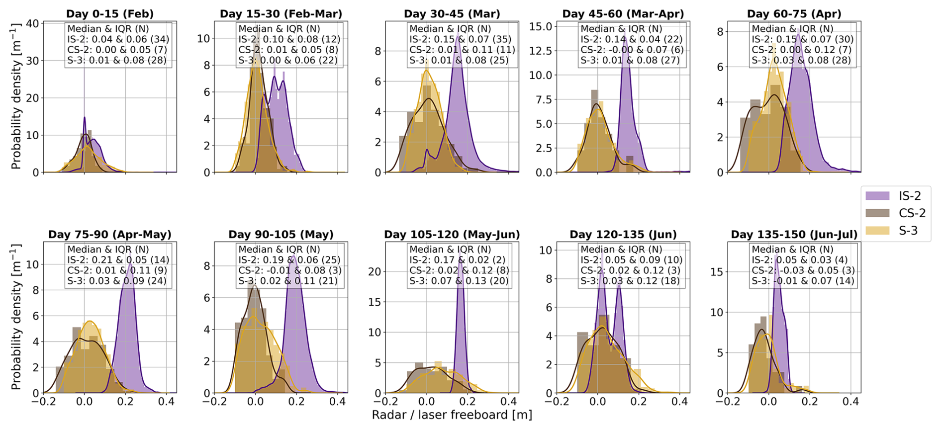
Figure 7 The evolution of laser and radar freeboard distributions at 15-d intervals for FYI. Distributions are estimated using all along-track freeboards samples inside the ROIs, i.e. before any spatial averaging is performed. N stands for the number of tracks feeding into the distribution.

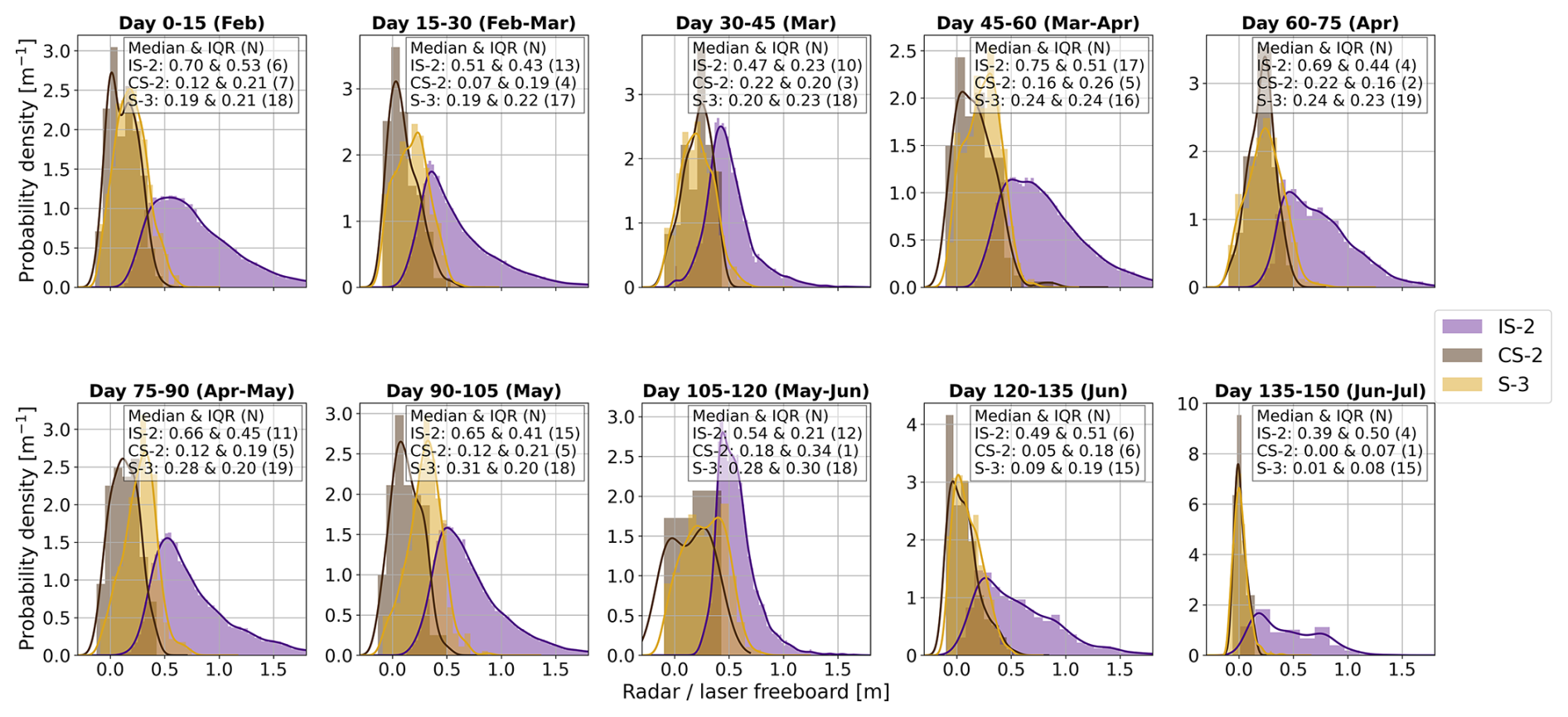
Figure 8 The evolution of laser and radar freeboard distributions at 15-d intervals for MYI. Note the scale difference on the x-axis compared to the FYI distributions in Fig. 7. Distributions are estimated using all along-track freeboards samples inside the ROIs, i.e. before any spatial averaging is performed. N stands for the number of tracks feeding into the distribution.

The MYI regions have already accumulated snow over the course of several months before we start tracking them in February. This is reflected in laser freeboards that are consistently 0.3–0.4 m higher than the radar freeboards during the winter period. Laser freeboards initially drop from ∼ 0.6 to ∼ 0.4 m, before rising and stabilizing ∼ 0.6 m from 1 April until melt onset. Radar freeboards start in the range 0.1–0.2 m and then increase towards 0.3 m around 15 March. The freeboards then drop to ∼ 0.2 m before they rise again to 0.3 m in late April. The periods with higher radar freeboards are short (∼ 7–10 d) and coincide with periods of warmer air temperatures (T > −15 °C) and snowfall. At melt onset, freeboards gradually start decreasing for both sensors. The rate of decrease is higher for radar freeboards (−0.93 cm d⁻¹) than for laser freeboards (−0.56 cm d⁻¹), although it must be noted that only two IS-2 crossings are available in the melt onset time period. The radar freeboards stabilize at values close to zero by the start of advanced melt, while the laser freeboards continue decreasing for another 20 d in advanced melt.

In Figs. 7 and 8 the evolutions of the laser and radar freeboards are visualized as distributions per 15-d time intervals for FYI and MYI, respectively. Note that these distributions are estimated using all along-track laser and radar freeboards sampled inside the ROIs, so before any spatial averaging is performed. Radar freeboard distributions are drawn separately for CS-2 and S-3 to examine the consistency of freeboards obtained from these different sensors. For FYI the distributions neatly capture the cycle of a seasonal ice cover: initial ice formation (day 0–15), followed by a period of ice growth and rapid snow accumulation (day 15–60), slowed ice growth and snow accumulation (day 60–105), and eventually melt (day 105–150). In the stage of initial ice formation (day 0–15) the laser and radar distributions are peaky, with lowest IQRs, and overlap with a median freeboard close to zero. It is notable that the laser freeboards thicken rapidly and are separated from the laser freeboards after only ∼ 2 weeks. In the period of ice growth and snow accumulation (day 15–105), the laser freeboards increasingly shift towards higher values, while the radar freeboards first remain relatively constant and low and only show a slight increase towards the end of the winter period. For both frequencies the inter-quartile range (IQR) increases though. During early melt onset (day 105–120) we observe a drop in laser freeboards and a narrower distribution, while the radar freeboards show an increase in median value and even more so in variance. Later during melt onset (day 120–135), a bimodal distribution is observed for the laser freeboards. We suspect this 15-d time window captures the period of snow ablation, including ten IS-2 crossings. The right-hand peak represents the higher freeboard returns from ice that is still covered by snow and coincides with the distribution seen in the previous 15-d period (day 105–120). The left-hand peak represents the lower freeboard returns after snow has melted and coincides with the distribution seen in the following 15-d period. In advanced melt, both the laser and radar freeboards continue decreasing towards zero.

The freeboard distributions over MYI (Fig. 8) clearly reflect the different seasons. Note the scale difference on the x-axis compared to the FYI distributions. The winter period shows a relatively stable situation with median laser freeboards well above the radar freeboards. The distributions have a much higher IQR compared to FYI, especially for the laser observations. This can be attributed to the more varied and deformed ice present in the MYI class, compared to only very smooth level ice in the FYI class. The transition towards melt onset (day 105–135) and advanced melt (day 135+) is characterized by increasingly narrow radar freeboard distributions, in combination with lower radar freeboard values. The laser freeboards maintain a large spread, but the mode clearly shifts towards lower values. Over the entire time series the laser distributions have a large IQR and positive skew, with the long tail representing the fraction of (heavily) deformed ice.

Generally speaking, the freeboard distributions derived from CS-2 and S-3 are in good agreement considering median freeboard and shape of the distribution for both ice types; confirming that freeboards from both sensors can be used interchangeably. Even in the 15-d periods where CS-2 has sparse coverage (low track density N), the resulting freeboard distribution consistently aligns very tightly with the independent S-3 distribution. This excellent cross-sensor agreement indicates that the spatial sampling by the radars remains highly representative even at low sample sizes. Due to the finer footprint size of the laser altimeter IS-2, distributions estimated in time windows with lower track density (N) are more likely to suffer from representation issues and should thus be interpreted carefully. Figure B1 in the Appendix summarizes the key statistics of the distributions over time. This figure shows that generally both the laser and radar distributions of MYI have a higher median and IQR than the FYI distributions. Meanwhile, a positive skew and Kurtosis (samples are closely centered around the mean with only few outliers) seem characteristic of a typical laser freeboard distribution, regardless of ice type. In contrast, the radar freeboard distributions are typically less skewed and have a low kurtosis (broader, flatter distributions).

5.3 Dielectric properties of the basal snow layer in the transition from winter to melt onset

Figure 6d and e show the modeled complex dielectric of the basal snow layer for a saline (FYI) snow cover and fresh (MYI) snow cover, respectively. We defined the basal layer as the bottom 10 % of the snow pack height, which in this study corresponds to an average height of 2 cm for FYI and 3.5 cm for MYI. In early May the basal snow temperatures are around −12 °C and the dielectric has similar values for both saline and fresh snow. Throughout May the basal snow temperatures follow an ∼ linear positive trend. The dielectric of saline (FYI) snow has a slight positive linear trend in the first half of May followed by an exponential trend in the second half of May. The transition to the exponential regime coincides with basal snow temperatures rising above −8 °C. In the range −8 to −3 °C the complex dielectric is very sensitive to minor temperature changes, as a small temperature shift in this range translates to a large change in liquid water content if the snow is saline. Meanwhile, the complex dielectric of fresh (MYI) basal snow remains constant across the observed range of snow temperatures, i.e. −15 to 0 °C. The increasing values of the complex dielectric constant result in reduced Ku-band radar penetration depth into the basal snow layer on FYI. However, in contrast to the nonlinear increase in the dielectric constant, the radar penetration depth reduces at a more constant rate throughout the entire month of May, going from ∼ 4 cm at −10 °C to <  1 cm at −3 °C. This implies that, theoretically, there is full penetration of radar waves in the saline basal layer on FYI in early May, followed by a rapid transition towards zero penetration right after melt onset in late May. Radar penetration in the fresh snow on MYI is stable and in the order of meters, meaning that theoretically the radar waves fully penetrate the basal snow layer as long as snow temperatures are below the freezing point.

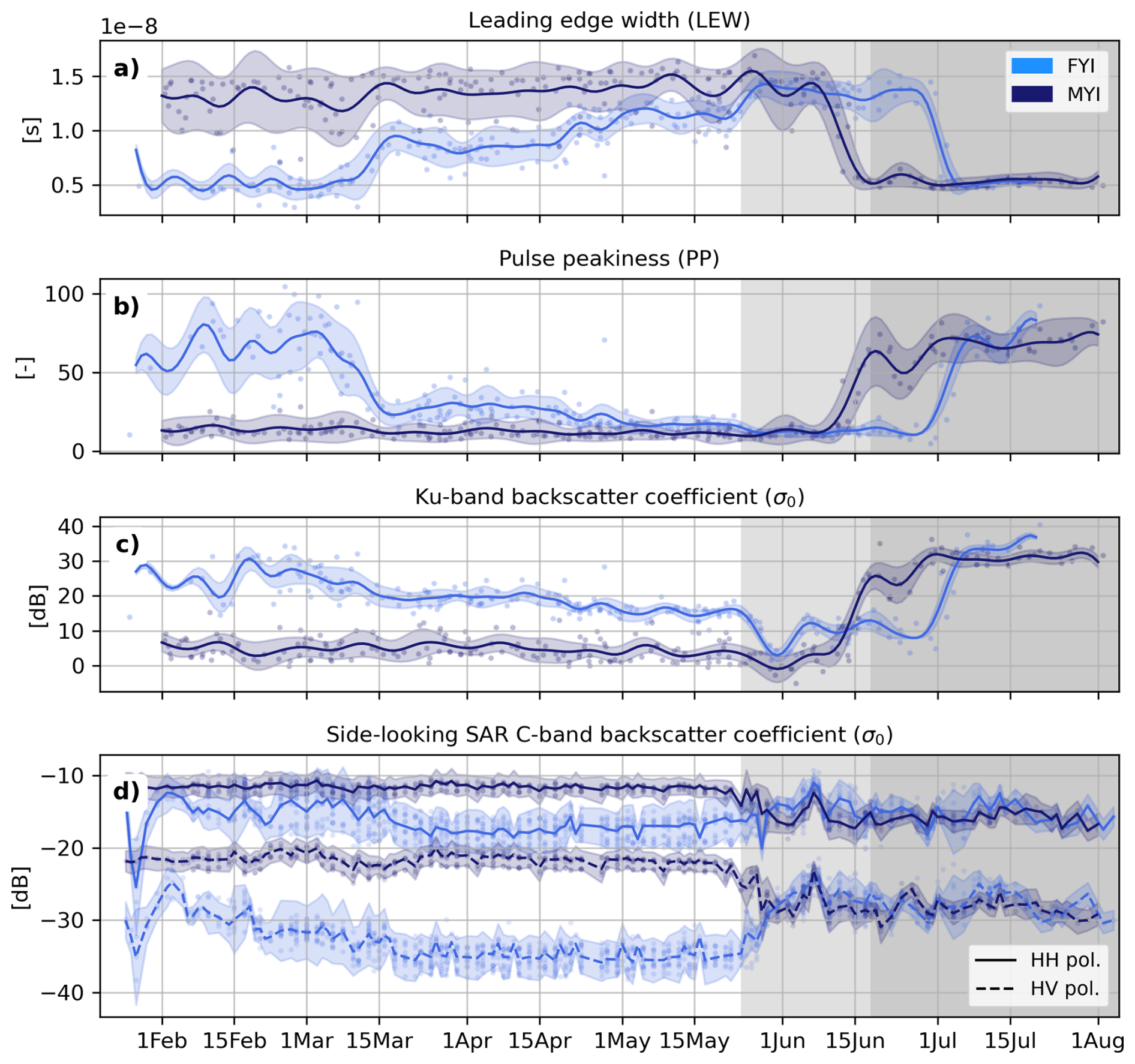
Figure 9 Seasonal evolution of a selection of radar waveform parameters over FYI and MYI (a–c), and seasonal evolution of the C-band SAR backscatter coefficient of the side-looking Sentinel-1 SAR sensor, for both ice types and imaging polarizations (d).

5.4 Seasonal evolution of radar waveform parameters

The evolution of a selection of Ku-band radar waveform parameters and C-band SAR backscatter coefficient is visualized in Fig. 9. From top to bottom the following parameters are shown: leading edge width (LEW), pulse peakiness (PP), radar backscatter coefficient (σ₀) in decibels for nadir Ku-band and side-looking SAR C-band. Parameters over MYI are stable throughout winter, with a low variance on the PP and σ₀, and higher variance on the LEW. The latter highlights that the MYI is significantly rougher than the FYI, and that the roughness varies across ROIs. Over FYI, the first 2–3 months after ice formation all parameters have distinctly different values than over MYI. Then, between 1–15 March, a sharp transition happens towards values closer to those observed over MYI. Afterwards, FYI parameters remain stable for a month before tending even closer to values observed over MYI towards the end of winter. More specifically, the LEW over FYI increases throughout the winter while the PP decreases. Since the ice is immobile and not deforming on the meters-scale, this is indicative of changes in the small-scale surface roughness of the ice and/or changes in the overlying snow cover. Interestingly, the LEW and its variance are very low over newly-formed sea ice, but increase significantly over the winter period. During melt onset the FYI parameters continue to evolve along the winter trends, while MYI parameters make a sudden jump in the transition towards advanced melt. The FYI parameters make the same jump with a 2 week delay (i.e. at the start of July) – well into advanced melt. Note how the FYI waveform parameters in advanced melt reach values similar to the ones seen at the time of initial ice formation.

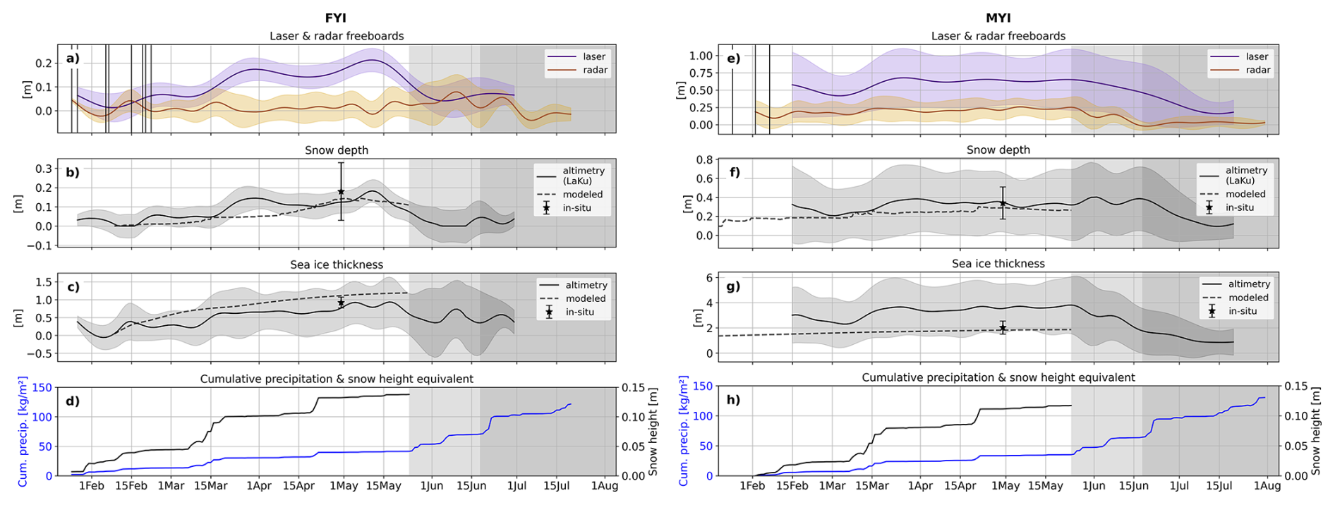
Figure 10 Panels (a–c) (FYI) and (e–g) (MYI): freeboards, snow depth, and sea ice thickness derived from dual-altimetry observations, numerical modeling, and in situ measurements. Shaded areas represent the inter-quartile range (IQR). Panels (d) (FYI) and (h) (MYI): cumulative precipitation and corresponding snow height equivalent from CARRA reanalysis.

The backscatter from SAR and altimetry should not be expected to correlate very closely, due to the different sensing geometries and frequencies, but the observations reveal similar patterns between frequencies. The seasonal evolution of C-band SAR backscatter over Arctic sea ice has been extensively studied, but the evolution of nadir Ku-band backscatter from satellite observations of the same ice has, to our knowledge, not been shown before with this temporal resolution. For FYI the ∼ 2 week-long ice formation period is characterized by a U-shaped variation in backscatter at both C- and Ku-band. The effects around ice formation are smeared out here because the parameters are visualized in absolute time. The backscatter values decrease and stabilize after ∼ 2 months at C-band, while Ku-band backscatter keeps decreasing throughout the winter period, with a steep decline from ∼ 30 to 20 dB between 15 February–15 March, followed by a stable period and then slower decline towards 15 dB right before melt onset. At melt onset the backscatter over FYI rises in C-band and remains at similar values during advanced melt. At Ku-band the backscatter further decreases during melt onset before making a sudden jump from 10 to 30 dB in the advanced melt period (early July). Over MYI the backscatter coefficients are relatively constant during winter for both frequencies, with the SAR C-band backscatter ∼ 6 and 12 dB higher over MYI than FYI for HH- and HV-polarization, respectively, and in contrast nadir Ku-band ∼ 15 dB higher over FYI than MYI. At melt onset C-band backscatter for MYI drops and stabilizes at similar values as for FYI, while Ku-band backscatter first remains low and then shows a sudden increase from ∼ 5 to 30 dB in the transition towards advanced melt, so ∼ 2 weeks earlier than the jump observed over FYI.

5.5 Seasonal evolution of dual-altimetry snow depth and sea ice thickness

Figure 10 shows the temporal evolution of laser and radar freeboards in absolute time, and derived SD and SIT for FYI (Fig. 10a–c) and MYI (Fig. 10e–g). Shaded areas represent the inter-quartile range (IQR) of these variables. Figure 10d and h show the cumulative precipitation and snow height equivalent. The SD and SIT are derived in two different ways: from LaKu dual-altimetry and from the snow/ice model.

Over FYI the LaKu SD is ∼ 0 cm when the ice forms, but it should be noted that small negative depth values at the start of the time series – due to radar freeboards being higher than laser freeboards – were set to zero to avoid using physically impossible snow depths in the SIT calculations. The SD increases stepwise throughout winter until reaching a maximum around 15 May with a median of 18 ± 6 cm. The major precipitation events (Fig. 10d) are reflected in the LaKu snow accumulation, albeit sometimes with a delay of 7–15 d, which is partly due to the interpolation scheme used to create the freeboard time series at daily resolution. The modeled SD is below the LaKu SD during most of the winter period and predicts a more continuous snow accumulation compared to the LaKu product. The higher snow accumulation rate over young ice might be caused by wind redistribution of snow, which is not well captured in the snow/ice model. The in situ snow depth measured on 29 April was 18 cm, which is 5 cm higher than the median LaKu SD on that day, but within the IQR. Furthermore, the cumulative snow height equivalent from reanalysis (14 cm) is in good agreement with the maximal LaKu SD (18 cm) reached towards the end of the winter period.

The median FYI SIT (Fig. 10c) starts at ∼ 0.4 m, due to the initially high radar freeboards, then quickly drops down to 0 m before increasing to a maximum of ∼ 0.9 m in early May. During winter the thickness increases at a relatively steady rate, except for the rapid ∼ 0.4 m increase seen in mid-March, which coincides with the warming event and strong snowfall. The in situ SIT measured on 29 April was 0.92 m, which is in good agreement with the dual-altimetry SIT of ∼ 0.8 ± 0.5 m. The modeled SIT shows a steeper ice growth rate of 1.3 cm d⁻¹ compared to the dual-altimetry of 1 cm d⁻¹, leading to a difference of ∼ 0.25 m in early May, and a maximal difference of ∼ 0.4 m in the middle of May. The higher ice growth rate is a direct consequence of the lower volume of modeled snow accumulation up to mid-April, leading to less insulation between the cold atmosphere and the underlying ocean and therefore increasing thermodynamic ice growth.

Figure 10e–h show the same variables over MYI. Note the large scale differences on the y-axis between the FYI and MYI plots. The LaKu snow depth over MYI (Fig. 10f) varies between ∼ 0.3–0.4 m over the winter period, apart for a short time around 1 March when it decreases down to 0.2 m. The modeled snow depth is on average 5–10 cm below the LaKu snow depth during the winter period; a similar offset as seen over FYI. LaKu snow depth is in very good agreement with the in situ measured depth of 0.34 cm in late April. During melt onset the LaKu snow depth remains high, as both the laser and radar freeboards decline at similar rates, and precipitation events are potentially still falling as snow. Advanced melt is marked by a rapid decline of −1.2 cm d⁻¹ in snow depth.

Altimetry-derived SIT for MYI (Fig. 10g) is relatively stable throughout the winter period at ∼ 3.7 m, followed by an approximately linear decline in melt onset and early advanced melt, at a rate of −6.6 cm d⁻¹. The only larger fluctuation in SIT is seen around mid-March (warming event), when SIT first drops to ∼ 2.3 m and increases to ∼ 3.7 m over the course of 15 d. The modeled SIT is 1.5–2 m thinner than the altimetry-derived values, and so is the in situ SIT measured on 29 April. The ice growth rate during winter is 1 cm d⁻¹ in the altimetry-derived product compared to 0.2 cm d⁻¹ in the modeling output, even though the altimetry-derived SIT is significantly thicker and has a deeper snow cover. Compared to FYI, a major difference is apparent in the trends at melt onset when SIT rises over FYI while it decreases over MYI.

6 Discussion

The time series shows that, during winter, the retracked heights of laser observations are distinctly higher than those of Ku-band radar observations, for both FYI and MYI. Median laser freeboards are ∼ 0.15 m (FYI) and ∼ 0.4 m (MYI) higher than median radar freeboards, with little overlap between the IQR envelopes. The only exception is seen over newly-formed ice, where radar freeboards exceed laser freeboards. This indicates that during winter the retracked heights at Ku-band frequency correspond to locations below the air/snow interface. The reference in situ observations are only available in late April and May, at the seasonal peak of ice thickness. For the FYI ROIs in this study, the in situ observations therefore represent an end member from which we can evaluate the full FYI time series. We know the ice and snow thickness start at zero, and we know that both variables approximately match the in situ measured seasonal peak in April–May. We can therefore assess fluctuations in the FYI time series relative to these seasonal end members. In addition, we use the modeled SIT as reference for the expected thermodynamic growth. In this context, we observe that during winter the retracked heights at Ku-band frequency correspond to locations well below the air/snow interface, for both ice types. These results do, of course, depend on the radar freeboard processing chain. For the processor used here, which applies the LARM retracker, we find that the FYI radar freeboards trace the snow/ice interface during ∼ 85 % of the winter time. This fraction corresponds to the amount of days the radar freeboards follow the monotonous, slight positive trend corresponding to the thermodynamic ice growth compared to the total amount of days in the winter period. This finding is consistent with the assumption that Ku-band radar waves fully penetrate through cold snow and that the dominant return originates from surface scattering at the snow/ice interface. Over MYI we are not able to reliably assess the location of the retracked heights relative to the snow/ice interface, because we do not have the same start and end references as for FYI, but we find that the minimal penetration depth into the snow is 40 % (see Sect. B1 in the Appendix). However, we also observe periods with elevated radar freeboards at different moments in the winter and melt season, for both ice types. During winter these periods are short (∼ 7–10 d), and generally coincide with periods of higher temperatures and snowfall. During the melt season the elevated radar freeboards are only seen over FYI. A temporary increase in radar freeboard can either be the result of a physical increase in the ice freeboard, or a measurement bias. Note that in this study, we defined radar freeboard as the waveform-derived estimate of ice freeboard without correction for the delayed radar wave propagation in the snow. Thus, the derived radar freeboard can be biased if it does not correspond to the ice freeboard after applying the delay correction. This can happen when relative contributions from surface scattering at the air/snow interface or snow volume scattering become equally or more dominant than the relative contribution from the snow/ice interface return in the detected waveform. Alternatively, such a bias can be introduced by processing choices during retracking. These two sources of bias can also be connected if real changes in the balance of snow and ice scattering returns invalidate the assumption of a dominant return originating from the ice surface. A broadening of the radar waveform by increased snow scattering is then artificially attributed to surface roughening by the retracker, resulting in the retracking threshold being biased low (height biased high). It is typically challenging to fully separate the impact of changing scattering processes versus the impact of the retracker on an observed bias, unless a sensitivity analysis is performed using different retrackers.

The findings presented here are based on radar freeboards obtained with the LARM retracker, and are therefore not instantly applicable to freeboards obtained with other retrackers. Nevertheless, since height estimates from both physical and empirical retrackers are affected by changes in waveform shape as well as range, we expect the relative variations in our time series to appear similarly for empirical retrackers, even though their magnitudes could be different. The retracker is not the only processing step that can affect the height estimates; the lead classification and SSHA interpolation routines may also. It is beyond the scope of the study to investigate the sensitivity of the results to all possible processing steps. For now, the findings are only proven for radar freeboards retracked with LARM. The data set of this case study is publicly available and can thus be used as a starting point to test the impact of e.g. different retrackers, classification algorithms, SSHA interpolation routines, snow depth and ice density products against a controlled reference time series.

6.1 Temporary increase in radar freeboard: physical increase or measurement bias?

The ice we track is entirely immobile throughout the presented time series, and thus experiences minimal to no dynamic thickening. If the 4 cm increase in FYI radar freeboard seen during the warming event in mid-March was a physical increase in freeboard, this would imply ∼ 0.4 m thermodynamic ice growth in 10 d. Such rapid ice growth would require extremely cold conditions, which is not the case during the warming event. In addition, there is ∼ 5 cm snow accumulation during this 10 d time period (see Fig. 10d), which should reduce the physical freeboard. Theoretically, each cm of snow accumulated leads to an instantaneous 0.54 cm decrease in radar freeboard, for a snow density of 300 kg m⁻³(Nab et al., 2023). In our time series, this would translate to a 2.7 cm decrease in radar freeboards during the warming event in mid-March. The fact that we see a 4 cm increase instead implies the presence of a strong counteracting mechanism. We are not aware of any physical mechanism that could temporarily raise the physical freeboard as much, and therefore suspect this increase to be a measurement bias. The same argument holds for the temporary increases in radar freeboard observed over MYI (up to 10 cm), which also coincide with periods of warmer temperatures and heavy snowfall. The time series of in situ snow and ice thickness from the SIMBA buoy is only available over MYI for one month in April–May, and there is no increase in altimetry-derived radar freeboards over MYI in this period. Thus, we cannot use the in-situ time series to verify whether the increases in radar freeboard seen during winter are nonphysical, or represent actual changes in the ice freeboard. Nevertheless, we converted in situ snow and ice thickness from the SIMBA buoy to laser and radar freeboards (see Fig. B3 in the Appendix). This time series confirms that MYI freeboards are relatively constant in May.

A radar altimetry waveform must be retracked to obtain a precise range measurement. Since the retracking point is directly linked to the shape of the waveform, it can be challenging to assess whether a temporary positive bias corresponds to a deviation in the scattering processes in the snow and ice from the assumed behavior at Ku-band, or if it is an artifact introduced purely by the retracker. By careful inter-comparison of the time series of radar freeboards, radar waveform parameters, and C-band SAR backscatter, we find pieces of evidence pointing towards the fact that the temporarily biased radar freeboards seem to originate (at least partly) from changes in the scattering processes of the snow and ice, rather than being introduced purely by the retracker. One of the parameters optimized by LARM is the surface topography root-mean-square (RMS) height, or more explicitly the RMS of the radar scattering distribution if it is not just a single surface contributing to the detected waveform. Changes in the effective RMS height thus indicate changes in the shape of the waveform (broadening/narrowing), which may result from changes in the surface roughness, but may also result from changes in snow scattering mechanisms that are not captured in the LARM waveform model. Figure B5 in the Appendix shows the seasonal evolution of the effective RMS height for FYI and MYI. For MYI we see that the effective RMS height closely follows the patterns of atmospheric conditions during the winter: periods with warmer temperatures and heavy snowfall have a higher effective RMS height, i.e. broader waveforms. These are the periods when we observe heightened radar freeboards over MYI. Remarkably, no concurrent changes in other waveform parameters or Ku-band backscatter are observed for MYI, though there is a temporary decrease in C-band SAR backscatter in the HV-polarization during the mid-March warming event and in the period leading up to melt onset. A drop in SAR HV-polarized backscatter indicates a decrease in volume scattering, and increased effective RMS height indicates the waveform has broadened. The fact that two independent sensors observe a change is a strong indicator that the temporary increases in radar freeboard over MYI are caused by changes in the scattering processes on the surface. For FYI we also see an increase in effective RMS height in periods of higher temperatures and snowfall, but the increase is less pronounced and not of temporary nature (Fig. B5). We see a first slight increase in effective RMS height during the warming event in mid-March, when the newly-formed ice first gets snow-covered. In contrast to the radar freeboards that decrease again after the warming event, the increase in effective RMS height remains, i.e. waveforms stay broadened. We observe a large, concurrent shift across all waveform parameters for FYI, and a decrease in nadir Ku-band and C-band SAR backscatter. Again, the fact that we see a simultaneous change in the C-band SAR backscatter indicates that the rise in FYI radar freeboards likely originates from a change in the scattering processes in the snow and ice.

In summary, we observe temporary increases in radar freeboard that cannot be linked to physical increases of the ice freeboard, and we see concurrent changes in C-band SAR backscatter. It is most likely that the temporary increases in radar freeboard are measurement biases arising when the scattering processes in the snow and ice do not correspond to the assumed full snow penetration of Ku-band radar waves and a dominant return originating from the snow/ice interface. In these cases, the basic assumption of the retracker is invalidated and artificial broadening of the radar waveform by scattering across a larger RMS height means that the retracking threshold is biased low and retracked height biased high. Temperature is a key driver of changes in the dielectric snow properties that affect the propagation of Ku-band radar waves, because it governs the liquid water content in the snow (Nandan et al., 2020). We therefore discuss the interaction of radar waves with snow in cold versus warm conditions and examine the implications for radar freeboard retrievals, as well as dual-altimetry snow depth and ice thickness products. The distinction between cold and warm conditions cannot be set by a generic, fixed temperature threshold, because other snow characteristics, such as salinity, influence the dielectric snow properties. In the time series studied here, we observe the transition from cold to warm conditions when air temperature rise above −10 °C.

6.2 Radar freeboard retrievals in cold conditions

By careful analysis of the time series we identify three situations that can lead to overestimated Ku-band radar freeboards in cold conditions, i.e. the retracked heights do not trace the snow/ice interface but a location higher up in the snow.

Newly-formed ice

At the moment of ice formation we expect the laser and radar returns to produce equally low freeboards, as there is no snow cover yet and both sensors should observe the same surface. However, we observe spuriously increased freeboards for both frequencies. High Ku-band freeboards are notably seen only in the Northern FYI ROIs (not shown here), but impact the full FYI area-averaged freeboards in the first 1–2 weeks after ice formation. As there is no snow cover on the ice yet that can bias the freeboard retrievals, we suspect this bias to originate from: (i) ocean wave effects, (ii) the retracking process and/or (iii) ice properties during formation. At the very onset of ice formation, the high LEW and low PP values suggest ice forming in ocean swells (Zhu et al., 2024). On a slightly longer timescale, the Ku-σ₀ time series show a U-shaped change over FYI in the weeks of ice formation (25 January–20 February), which likely represents the formation and decay of frost flowers on the new ice. These features significantly increase the roughness at centimeter-scale and thus increase scattering at the air/ice interface, which leads to broader waveform returns (Landy et al., 2020). We observe this effect in the radar waveform parameters: periods of lower Ku-band backscatter are accompanied by lower PP and higher LEW (note that the effect is smeared out since the waveform parameters are displayed in absolute time). The broader waveforms might displace the tracking point up from the air/ice interface, as the two surface roughness parameters optimized in LARM (effective RMS height and radar wavelength-scale roughness) will get larger values and thus lower the retracking threshold. So, if frost flowers (with  0 large-scale topography) produce a very broad radar waveform, both roughness parameters are likely to be overestimated, leading to an artificially-lowered retracked range that biases freeboards high.

Saline basal snow layer

The radar modeling results suggest that Ku-band waves only penetrate 3–4 cm into snow with salinity values in the range 1–6 PSU for air temperatures in the range −15 to −10 °C and snow ∼ −10 °C. The 3–4 cm distance roughly corresponds to the average height above the snow/ice interface up to where saline snow was observed in situ, although Arctic-wide saline snow can be found up to 6–8 cm and at salinities in the range 0–20 PSU (Nandan et al., 2017). So, in case of a thicker saline basal layer (> 4 cm) and/or a highly saline basal layer (S > 6 PSU), the retracked height might not correspond to the location of the snow/ice interface but a location higher up in the snow, even in cold temperatures. This positive bias would be caused by increased radar wave absorption and/or volume scattering in the basal snow layer, which reduces the relative contribution of the snow/ice surface reflection in the detected waveform (Zhou et al., 2026).

Thick snow cover

Previous studies have pointed out that thick snow covers (> 20 cm) can displace the tracking point towards the altimeter and bias radar freeboards high, because returns from the air/snow interface significantly broaden the waveform (Kwok, 2014; Ricker et al., 2015). In this light, we suspect the thick snow cover on the MYI in this study (>30cm) to be biasing the radar freeboards high. This would contribute to the discrepancy between the altimetry-derived SIT of ∼ 3.7 m and the in situ measured SIT of 2 m. The actual SIT was most likely in between the in situ and altimetry-derived values, as the in situ SIT obtained from transects with the GEM and Magnaprobe were performed manually and therefore surveying the heavily deformed ice was unfeasible. In addition, we only have one transect of 1 km total that was made over MYI, whereas our polygons cover 1340 km²; well beyond the in situ sampling sites. The variability in IQR of altimetry crossings over MYI ROIs and wider distribution of in situ ice thickness data suggest that the thickness of MYI within the fast ice was highly variable. The vertical offset between the SIMBA-derived and altimetry-derived laser and radar freeboards also illustrates this (Fig. B3 in the Appendix). The discrepancy between altimetry and in situ SIT for MYI could therefore be entirely caused by representation issues. The thickest ice and snow is likely not well captured in the in situ measurements. Furthermore, we believe the correspondence between the modeled and in situ SIT is a coincidence, as the modeled SIT for MYI heavily relies on the assumed SIT at the modeling start date, which in our case was set to 0.3 m on 10 October 2021, as described in Sect. 4.8. Even though we suspect a high bias in the radar freeboards over the MYI areas, the difference between the laser and radar freeboard heights indicate that the retracked heights at Ku-band frequency correspond to locations well below the air/snow interface, with at least 40 % penetration into the snow during winter but likely much deeper (Sect. B1 in the Appendix).

6.3 Radar freeboard retrievals in warm conditions

We observe warm conditions at two distinct moments in the time series: during the winter warming events and during melt onset and advanced melt. The warming events are a temporary change from the cold winter baseline conditions, while the transition from winter to melt marks a shift of regimes that comes with more significant and lasting physical changes in the snow and ice. We therefore discuss both cases separately, even though some mechanisms are shared.

6.3.1 Warming event during winter

During the warming events around 15 March and 20 April, air temperatures are mainly in the range −10 to 0 °C and CARRA indicates snowfall. We observe concurrent, temporary increases in radar freeboard, with MYI radar freeboards temporarily increasing by 10 and 5 cm in response to 5 and 3 cm snow accumulation, respectively. Over FYI the radar freeboards rise from ∼ 0 to 4 cm during the snowfall event of 15 March, but no significant freeboard increase is visible for the event in April. For the warming event in mid-March, the 4 and 10 cm bias in radar freeboard translate to a relative increase in SIT of 160 % and 65 % for FYI and MYI, respectively. It is unlikely the freeboard rises are data artefacts, since they are all evident in several independent altimeter crossings from CS-2, S-3A and S-3B. At both occurrences, FYI waveform parameters drastically change, with LEW increasing while PP decreases, and the C-band backscatter over FYI drops by ∼ 5 dB. These findings indicate major geophysical changes in the snow cover over FYI. Interestingly, no significant changes are observed in the MYI waveform parameters and SAR backscatter, except for a small increase in LEW.

Strong snowfall

We observe that radar freeboards increase during periods of snowfall and stay heightened for ∼ 1 week afterwards before returning to pre-snowfall values. These observations contradict the common understanding that snow loading weighs the ice down, which should result in a decrease in radar freeboards. As outlined in Sect. 6.1, the ∼ 5 cm snow accumulation during the mid-March winter warming should theoretically lead to a decrease in radar freeboards of ∼ 2.7 cm. However, the opposite is observed with FYI and MYI radar freeboards rising from ∼ 0 to 4 cm and from ∼ 15 to 25 cm, respectively (see Fig. 6b and c). A scatterplot showing precipitation anomaly versus radar freeboard anomaly confirms a positive correlation between precipitation anomaly and radar freeboard for both ice types, see Fig. B4 in the Appendix. The temporary increase in freeboard suggests that there is a shift in the (relative) contributions of different scattering interfaces to the detected waveform, with a relatively higher contribution of radar returns originating from above the snow/ice interface during and right after periods of snowfall, which is in line with the findings of Gregory et al. (2021), Nab et al. (2023). Snowfall events often coincide with warmer air temperatures, but the freeboards tend to stay elevated longer than the temperatures do.

The temporary change in scattering contributions is suspected to, at least partly, come from changes in the roughness of the air/snow interface (Nab et al., 2023), at scales corresponding to snow features (dunes, drifts) and micro topography down to the radar wavelength (mm–cm roughness) (Landy et al., 2026). Additionally, wind packing might increase the density of the upper snow layers. Most snow pits sampled in situ in late April had a dense upper half and softer bottom half structure, confirming wind packing happened in our study region. These surface roughness and snow density changes can redress the balance of Ku-band radar scattering between snow/ice and air/snow interfaces, since a change in the dielectric contrast across the air/snow interface or smoothening of the radar roughness could enhance scattering from the snow surface (Landy et al., 2026). This could be caused by wind redistribution of snow and snow property changes during a storm (Nab et al., 2023; Nandan et al., 2023). Notably, the waveform parameters over FYI show an increase in LEW and decrease in PP and Ku backscatter during the major snowfall events in mid-March and late April, indicating the radar waveform broadens in direct response to snow accumulation and snow surface changes, as was also found in Khvorostovsky et al. (2020). An enhanced radar return from the air/snow interface relative to the snow/ice would broaden the detected waveform sampled at the satellite range resolution (47 cm). The waveform parameters do not return to pre-snowfall values afterwards, indicating that lasting physical changes are introduced in the snow cover during a strong snowfall event, but the radar freeboards do return. Interestingly, the MYI waveform parameters do not change in response to strong snowfall, except for a small increase in LEW. Compared to the FYI, the ice surface of MYI is very rough on large scales and highly heterogeneous within the altimeter footprint. As a result, the returns from the snow/ice interface likely override the effects of changes in either snow surface roughness or internal snow properties over the MYI during storms. In contrast to the radar freeboards that decrease again to values observed before the warming event, the waveform parameters stabilize at the new values, indicating a lasting change is introduced on the snow and ice surface during the period with warmer temperatures and snowfall.

Saline basal snow layer

The fact that the radar freeboard increase is temporary whereas the waveform parameters change irreversibly points to the presence of a second mechanism rising the FYI radar freeboards in periods of warmer temperatures and precipitation. In addition, the relative increase in SIT observed in response to snowfall is smaller over MYI than over FYI (65 % vs 160 % increase). Snow on FYI typically has a saline bottom layer and a rise in temperature increases the brine volume fraction in this layer, even at temperatures below freezing point. Increased brine in the basal snow layer shifts it into the pendular saturation regime where water is contained in isolated pockets around the ice grains (Denoth, 1999), assuming that the microstructure of brine-wetted snow is similar to the microstructure of wet snow. Liquid water has a much higher dielectric loss factor than ice, leading to strong microwave absorption even at small brine volume fractions (Barber and Fung, 1998). In the presence of depth hoar crystals (which were observed in every sampled snow pit), the brine might coat the crystals and turn them into major scatterers at Ku-band frequency (Barber and Fung, 1998). This effect could shift the dominant radar scattering location up toward the altimeter and lead to overestimated radar freeboards (Nandan et al., 2017). However, the total absorption or volume scattering directed away from the radar needs to be high enough to overpower the quasi-specular reflection that is commonly observed for peaky FYI altimeter echoes and that is thought to originate from the relatively smooth snow/ice interface (De Rijke-Thomas et al., 2023). A more likely alternative is that the enhanced radar wave absorption in the saline snow layer suppresses the reflection from the snow/ice interface, thereby allowing the air/snow interface reflection (or snow internal interface reflections) to contribute significantly to the detected waveform, which biases the retracked freeboards high. The latter theory implies that the dominant radar backscatter originates from the interfaces rather than from snow grains in or above the basal layer, and is more consistent with in situ nadir Ku-band radar studies that mainly observe sharp peaks at the key interfaces (Willatt et al., 2011; Stroeve et al., 2020). This additional bias introduced by saline snow in warmer periods also supports the satellite-based findings of (Nab et al., 2023) that CS-2 radar freeboard sensitivity to air temperature seems stronger over FYI than MYI.

We conclude that the radar freeboard increase observed over FYI during warming events is likely the combined result of snow accumulation, changes in the snow surface roughness, and increased brine volume in the basal snow layer. This can lead to (i) increased volume scattering within the snow cover, and/or (ii) increased surface scattering at the air/snow interface, and/or (iii) increased microwave attenuation in the saline basal snow layer. The detected waveform is broadened as a result of the two-way radar attenuation inside the basal snow layer, which reduces the strength of the return from the snow/ice interface, in combination with either relatively or absolutely larger contributions from snow volume and snow surface scattering. The radar freeboard increase is temporary, while changes in the waveform parameters are permanent. We attribute this to the fact that snow surface roughness and density/hardness changes are more long-lasting, while a brine volume increase reverses when temperatures drop again after a warming event. Generally speaking, during winter the periods with biased radar freeboards are short (7–10 d) and in total only account for ∼ 15 % of the time (in this time series).

6.3.2 Melt season

At the start of melt onset (24 May) the laser and radar freeboards start dropping for MYI. Over FYI, however, radar freeboards rise while laser freeboards decline. This uptick in radar freeboards starts before melt onset, with the first elevated freeboards around 17 May, and lasts until 7 June. Radar freeboards rise by ∼ 10 cm in this time period, while air temperatures go from −10 to 0 °C and snow temperatures from −8 to 0 °C. Vertical snow temperature gradients from the SIMBA instrument reveal a transition period between mostly positive gradients to negative gradients between 16–22 May (Fig. B2 in the Appendix). This coincides with the appearance of the first elevated radar freeboards (individual crossings > 0.1 m), but no clear changes are seen in the waveform parameters before melt onset. At the start of melt onset, a change in C-band backscatter is observed over both FYI and MYI, implying geophysical changes in the properties of the snowpack across the entire study region (Karlsen et al., 2024). However, we only observe a concurrent change in nadir Ku-band backscatter over FYI, not over MYI which is relatively stable, with the LEW also changing for FYI. So, the changes in the snowpack evident in C-band SAR only seem to manifest as a clear change in waveform parameters over FYI. We evaluate different physical mechanisms that could be causing the Ku-band radar freeboards over FYI to increase around melt onset while FYI laser freeboards and MYI freeboards show the opposite behavior.

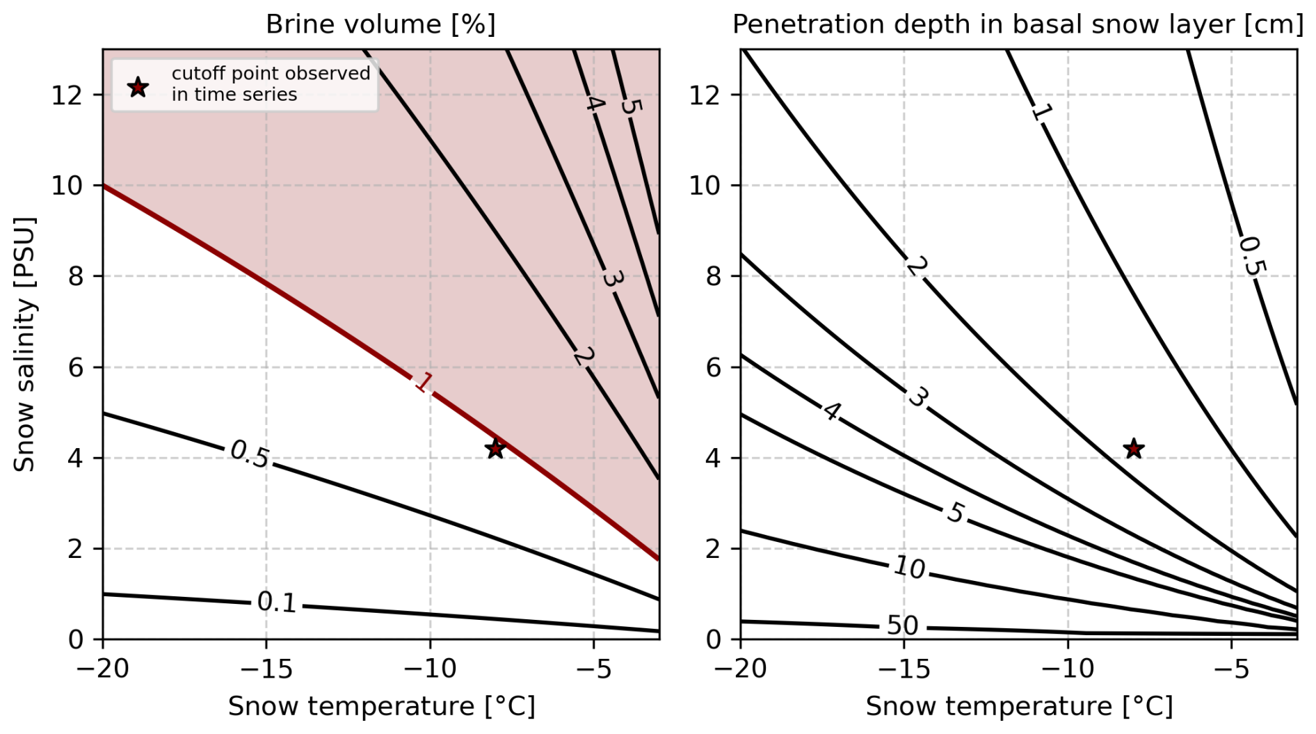
Figure 11 Modeled brine volume and Ku-band radar penetration depth into the basal snow layer (bottom 10 % of snow pack) for a range of typical Arctic snow temperature and salinity values, assuming a snow density of 310 kg m⁻³ (the median snow density for the FYI study sites in mid-May). Red shading is applied where combinations of temperature and salinity lead to a brine volume exceeding 1 %, which is empirically associated with high likelihood of biased radar freeboards. The cutoff point observed in the time series that led to this threshold is marked with a star.

Saline basal snow layer

The same mechanism as outlined for the warming event (Sect. 6.3.1) is also applicable at melt onset, i.e. warmer temperatures lead to increased brine volume fractions in the saline basal snow layer (defined here as the bottom 10 % of the total snow height) and hence increased microwave attenuation. In our time series, the uptick in radar freeboards around melt onset starts when basal snow temperatures increase above −8 °C. This coincides with the moment the modeled complex dielectric constant of saline snow transitions from linearly increasing to exponentially increasing (Fig. 6d). This temperature also corresponds to the eutectic point of sodium sulfate decahydrate (−8.2 °C) (Geldsetzer et al., 2009). The snow temperature of −8 °C in combination with a snow salinity of 4.2 PSU and snow density of 310 kg m⁻³ (i.e. the median salinity of the FYI snow pits and median FYI snow density in mid-May) corresponds to a brine volume of 0.94 %. Figure 11 shows the modeled brine volume and radar penetration depth into the basal snow layer for a range of typical snow temperature and salinity values found in snow on Arctic sea ice. The left panel of this figure shows the cutoff point in brine volume (0.94 %) that is observed in the time series studied here. From these empirical observations, we conclude that snow with a brine volume above 1 % is likely to introduce a positive bias in radar freeboards. To put these results in a more general context, we highlight the range of snow temperatures and salinities that result in a brine volume above 1 %. Note that this threshold of 1 % is a conservative estimate, since we use the median bulk snow density instead of layer-wise snow density due to the limited amount of layer-wise density measurements made in the snow pits. Observations of crystal type in the basal snow layer indicated the presence of depth hoar crystals, so the actual density of the basal snow layer was likely below the median bulk value of 310 kg m⁻³. For example, lowering the basal layer snow density to 250 kg m⁻³ while keeping the temperature and salinity values fixed leads to a brine volume of 0.76 % as cutoff point. The right panel in Fig. 11 shows that, theoretically, the Ku-band radar waves penetrate less than 2 cm into the 4.2 PSU basal snow layer at −8 °C. The empirical observation that brine volumes above 1 % are likely to bias radar freeboards high is in line with previous work reporting that at liquid water fractions above 0.01 the snow cover is dominated by the dielectric properties of the water over the properties of the dry snow (Howell et al., 2005). We do not have snow temperature data for the winter warming events, but we know that air temperatures approached zero degrees. It is thus likely that snow temperatures temporarily rose above −8 °C during these events, leading to a brine volume > 1 % in the basal snow layer on FYI which resulted in positively biased radar freeboards.

Wet snowpack

When temperatures remain positive for long enough, the entire snow column becomes saturated regardless of the presence of salts. This can lead to overestimated radar freeboards because Ku-band backscatter returns almost exclusively originate from the air/snow interface for a saturated snow pack (Howell et al., 2005). Large variability in retrieved freeboards on short time scales can occur due to diurnal thaw-freeze cycles that result in large differences in liquid water content during the day and night. This mechanism would impact both FYI and MYI.

Superimposed ice

The heightened radar freeboards at melt onset could also be caused by the formation of superimposed ice due to the refreezing of meltwater (Granskog et al., 2017). This would imply that the observed freeboards are not biased high, but in fact physically rise if we define the sea ice as including the superimposed ice. However, this mechanism would be likely to effect both FYI and MYI, although not necessarily at the same time due to differences in the snow radiation budget (and thus liquid water content) for snow packs of different depth, but we do not observe any freeboard increase during melt over MYI. We therefore conclude that there was likely no superimposed ice formation. Snow and ice thickness data from the SIMBA instrument that was deployed on MYI backs this up (Figs. B2 and B3 in the Appendix).

Melt ponds

The drainage of melt ponds can cause a rapid increase in ice freeboard (Salganik et al., 2025), but in our time series the ice is still pond free at the time we observe the increase in radar freeboards. The SIMBA instrument indicates that there is no snow ablation until 29 May (no data afterwards, see Fig. B2 in the Appendix) and Sentinel-2 optical imagery shows no ponds until at least 10 June 2022 (not shown here). The first image after a cloudy period shows ponded MYI on 27 June, while over FYI ponding increases between 30 June–3 July. We observe the first negative radar freeboards at the start of advanced melt, i.e. second half of June, which coincides with the appearance of the melt ponds over MYI. The ponds are highly reflective surfaces that dominate the radar echo and cause the retracker to overestimate the range (Armitage and Davidson, 2014), requiring specialized waveform classification and freeboard derivation algorithms (Braakmann-Folgmann et al., 2026). For MYI we see the first negative freeboards at the start of advanced melt, about 1 week after a large shift across all radar waveform parameters is observed. Over FYI the pond onset timing seems delayed by 2 weeks compared to MYI, since we observe the same patterns in waveform parameters and freeboards but with a 2 week delay. The optical imagery confirms this. The earlier timing over MYI may be caused by liquid water forming in refrozen melt ponds at the base of the snowpack (from the previous summer), creating highly reflective targets to the radar.

We conclude that the positive biases observed in FYI radar freeboards during melt onset are most likely caused by the saline snow, and potentially exacerbated by simultaneous snowfall. In summary, we observe periods with positively biased radar freeboards during winter and melt onset. During winter these periods are short, typically lasting ∼ 7–10 d, and biases are up to 4 cm for FYI and 10 cm for MYI. At melt onset the biases are only seen over FYI and are up to 10 cm. We believe these biases arise when scattering processes in the snow and ice deviate from the assumed behavior at the Ku-band wavelength, which is that the main radar return originates from surface scattering at the snow/ice interface. However, we do not have the data required to ascertain the exact magnitude of the biases, fully separate the drivers (i.e. warmer temperatures, snow accumulation, saline snow, or a combination of these factors), nor to quantify their relative contributions. The magnitude of the bias may also depend on the choice of retracker, so the values reported here relate specifically to the LARM algorithm. Bias magnitudes reported here are derived from the smoothed daily time series and therefore represent minimal estimates.

6.4 Implications for dual-altimetry snow depth and ice thickness retrievals from ice formation to melt

Our findings suggest that the assumption of full snow penetration at Ku-band frequency for SIT retrievals and dual-frequency altimetry snow depth retrievals is valid for ∼ 85 % of the winter period (in this time series). Still, more in situ validation data is needed at different times throughout the season and at larger scales to fully confirm this. We have only one tie point for validation, but this is near the end of the snow accumulation and ice growth seasons so it at least integrates processes affecting the ice since formation. The LaKu snow depth is within a few centimeters of the modeled snow depth at the end of the winter season. However, the LaKu snow depth shows a more rapid increase in the first weeks after ice formation compared to modeled snow accumulation, which might be caused by wind redistribution of snow. These findings are in line with previous studies reporting considerable snow deposition on newly-formed ice, particularly in the Atlantic sector of the Arctic where large cyclones are more common (Landy et al., 2026). Landy et al. find that the mean snow depth on new ice in the Atlantic sector is 14.9 cm within five days of formation. Over the newly-formed ice in our time series, we observe ∼ 5 cm snow cover within a week after formation, and ∼ 15 cm after one month.

The periods with biased radar freeboards impact the SD and SIT retrievals. The bias in radar freeboards observed over newly-formed ice leads to overestimated LaKu SD and SIT. It shows that correctly locating the retracking point on a waveform return over very smooth and thin ice (< 20–30 cm) remains difficult, so care should be taken when deriving LaKu SD and SIT over areas with a high fraction of young ice, such as the marginal ice zone or polynyas. Apart from the first weeks after ice formation, our results show that winter LaKu SD and SIT estimates obtained from Ku-band freeboards are reasonable as long as temperatures are cold. During winter, we advise caution for LaKu snow depth and SIT estimates derived (i) over FYI with a saline snow cover during warmer periods, (ii) during and immediately after strong snowfall. In the time series studied here, these cases make up ∼ 15 % of the winter period. In both cases Ku-band radar freeboards are likely to be biased high, resulting in underestimated snow depth and overestimated SIT values. The impact on SIT is largest, as a freeboard bias may magnify tenfold in the conversion to SIT if no other competing biases are present. The bias is particularly pronounced in the case of a winter warming event with snowfall over areas of FYI, because the different biases accumulate (although the extent to which they linearly add remains unclear). For the warming event observed in this study, the cumulative bias over FYI leads to a 160 % increase in ice thickness in just a few days. Similar artifacts are seen in altimetry-derived snow depth and ice thickness over FYI during melt onset, which leads to opposing trends in snow depth and ice thickness for FYI versus MYI. The lack of data in the advanced melt season bars the drawing of hard conclusions about LaKu snow depth and SIT at that time of the year; however, all freeboards are unrealistically thin over both ice types owing to melt pond biases (Landy et al., 2022).

7 Conclusions

We present a time series of laser and Ku-band radar freeboards from satellite altimetry over immobile regions of FYI and MYI ranging from mid-Winter to mid-Summer. For FYI this time series captures the entire seasonal cycle from ice formation to summer melt. Our analysis shows that, using the LARM retracker, the Ku-band radar freeboards over FYI trace the snow/ice interface during ∼ 85 % of the winter time. This supports the validity of the assumption that Ku-band radar waves fully penetrate through the snow and that the dominant return at nadir originates from surface scattering at the snow/ice interface during winter. Over MYI, the retracked heights correspond to locations well below the air/snow interface during winter, with at least 40 % penetration in the snow but likely much deeper, although the exact depth could not be reliable assessed. However, the data also provide evidence for periods with rapid increases in radar freeboard, during both the winter and the melt season. In the time series studied here, all cases of rapid increases in Ku-band radar freeboard appear to be biases rather than actual physical increases in freeboard. During winter, the biases are short-term, lasting ∼ 7–10 d, and have magnitudes of up to 4 cm for FYI and 10 cm for MYI. We suspect these biases to arise when scattering processes in the snow and ice deviate from the assumed behavior at the Ku-band wavelength, thereby reducing the relative contribution of the backscattered power from the snow/ice interface and allowing the backscattered power from the air/snow interface to weigh more in the detected waveform. This change in waveform shape acts to bias the retracking point low. Conventional sea ice retrackers are based on the assumption that the estimated retracking point represents the mean snow/ice interface elevation, but a change in waveform shape caused by atypical scattering processes invalidates this assumption. The choice of retracker may, however, increase or mitigate the magnitude of the bias. In most cases the bias coincides with specific atmospheric conditions that significantly change the physical and dielectric properties of the snow. In particular, our results suggest that, during winter, the Ku-band radar freeboards tend to be biased high: (i) for ice with a saline snow cover during a warming event (brine volume fraction > 1 %), and (ii) during and immediately after strong snowfall events. Additionally, there is the potential for a positive bias over MYI with a thick snow cover (> 30 cm), but this bias could not be reliably assessed from the data available in this study. Winter warming events are often accompanied by snowfall, leading to a cumulative bias for the areas with saline snow (i.e. most FYI in the Arctic). Here, the cumulative bias over FYI translates to a 160 % increase in ice thickness in just a few days, compared to only 65 % increase for MYI. In the period of melt onset in May/June, biased radar freeboards seem related to saline snow only, but biases are on average larger than during the winter period – up to 10 cm.

For the majority of the winter season (∼ 85 %), our findings support the assumption of full snow penetration and a dominant return from the snow/ice interface at Ku-band frequency for sea ice thickness retrievals, as well as for dual-altimetry snow depth retrievals, such as planned for the Copernicus Polar Ice and Snow Topography Altimeter (CRISTAL) mission (Kern et al., 2020). Though our results show evidence for short-term, positive biases in Ku-band radar freeboards under specific atmospheric conditions and physical snow properties, correctly identifying the freeboard samples that are affected and quantifying the magnitude of the bias remains a topic of investigation. This raises the proposition for flagging Ku-band freeboard samples with “probability of high bias” based on ice type and air temperature: FYI and T > −10 °C (i.e. saline snow cover in warm conditions). Dedicated validation campaigns will be needed to provide in situ snow depth and sea ice thickness data over the course of multiple weeks/months and at different times throughout the season. This could be achieved by deploying autonomous sea ice mass balance buoys on fast ice, as fast ice provides a more controllable test site that simplifies both the validation and the inter-comparison of different satellite sensors and observational frequencies.

Appendix A: Methods

A1 SAR incidence angle normalization

Wide-swath SAR sensors acquire data over a large range of incidence angles (IA), with small IA at near-range and a continuous increase in IA across the swath. As a result, the radar backscatter intensities typically decrease with increasing IA for the same surface type. For backscatter values expressed in decibels, the rate of decrease across the swath, i.e. the slope, is approximately linear. The steepness of the slope depends on the surface roughness and dielectric constant of the material being imaged (Ulaby et al., 1981). When investigating the backscatter evolution in a SAR time series that is not made up of repeat pass images, it is important to correct the backscatter values for variations in IA (Yackel and Barber, 2000; Makynen et al., 2003). This process is referred to as incidence angle normalization and implies finding a slope estimate and subsequently mapping all backscatter values to a common IA using this slope estimate. Slope estimates for sea ice can either be taken from literature, or derived from the SAR data itself if enough images over the same surface are available. Here, we estimate slopes from the SAR time series, as there are many images available and hence this should provide the most accurate slope estimate for the ice types inside our ROIs. We use the differencing method presented in Geldsetzer and Howell (2023) where a slope estimate is calculated for each successive pair of SAR images where the same ice is imaged at two different IA's. Following the method in Geldsetzer and Howell (2023), we estimate slopes per ice type for all pairs of images during freezing conditions and when the difference in IA is at least 7°. The average slope estimate per ice type and polarization is reported in Table A1. These values are then used to project the backscatter values onto a common IA of 35° for the entire SAR time series, also in the melt season.

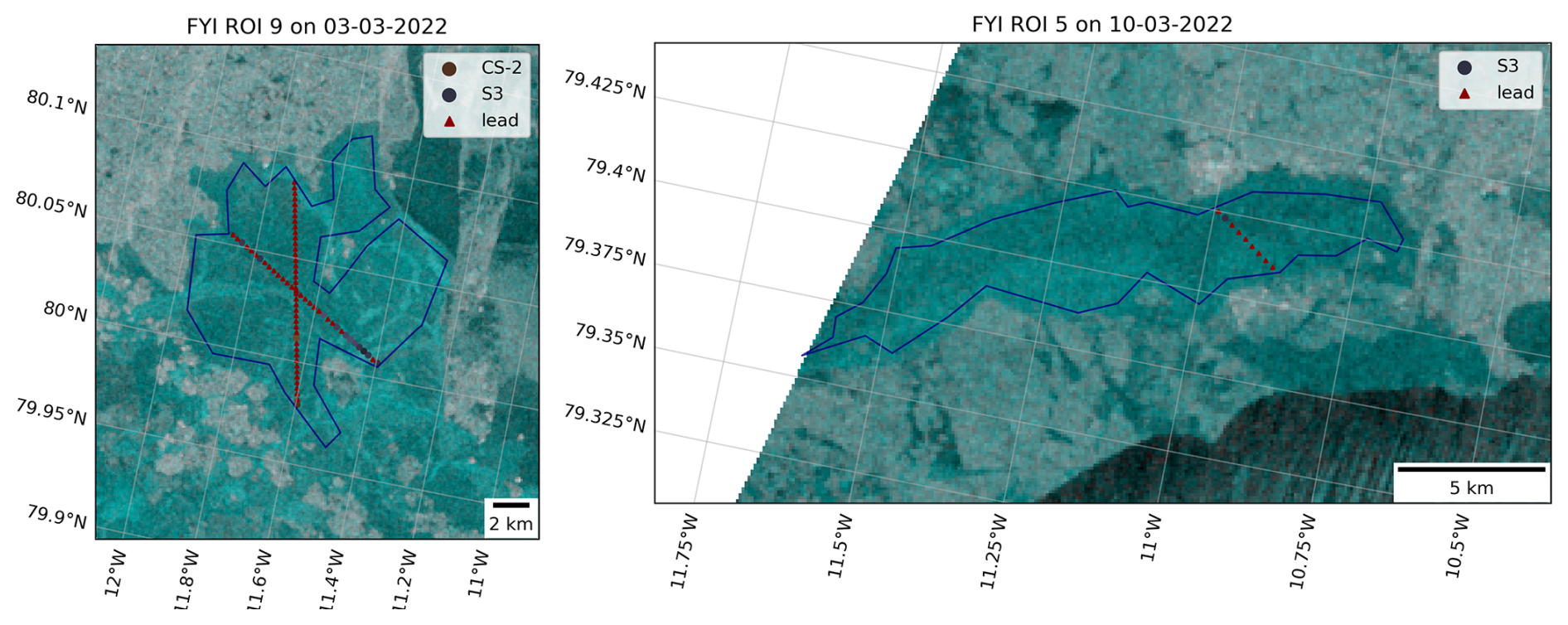
Figure A1 Two examples of the radar altimetry returns overlaid on temporally overlapping C-band SAR backscatter imagery. The SAR image is shown as false-color composite (HV-HH-HH polarization). Altimetry returns classified as lead are visualized with red triangular markers while returns classified as ice are shown in gray/brown circular markers. The ROIs are outlined in blue and in both examples the ice has already been growing for 3–4 weeks at the time of the data acquisition, so the lead returns are misclassifications.

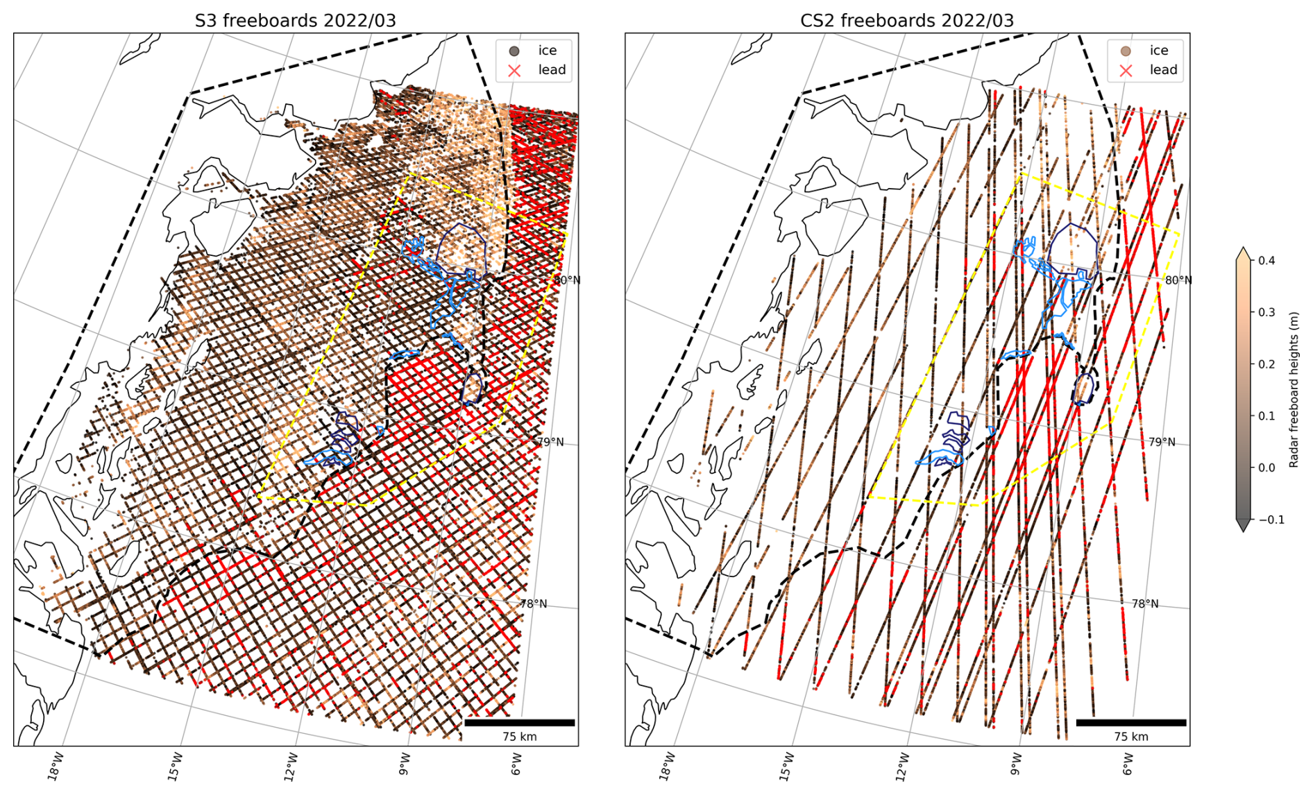
Figure A2 Map showing the radar freeboards acquired over the study region in March 2022 from the S-3 (left) and CS-2 (right) satellites, without masking “lead” returns inside the fast ice. Returns classified as “lead” are colored in red, while returns classified as “ice” have a radar freeboard value shown in brown shades. Note the amount of red markers, i.e. “lead” returns, inside the FYI ROIs and in other regions in the fast ice. Even though some of these might be actual leads, we decide to mask all lead returns in the fast ice to avoid introducing a bias in the radar freeboard calculations.

Table A1 SAR backscatter slope estimates in dB °⁻¹, per polarization and ice type.

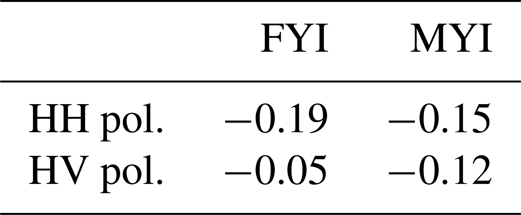
A2 Removing lead tie points over fast ice in along-track radar altimetry observations

We overlaid along-track altimetry returns on spatio-temporally overlapping C-band SAR images. Temporal overlap was defined as a maximum time difference of 24 h between the acquisition of a SAR image and an altimetry overpass. The visual aid of the SAR image helped to qualitatively interpret the altimetry data. It revealed that many radar waveform returns over the FYI ROIs in both CS-2 and S-3 were wrongly classified as lead, even weeks after the ice had initially formed. Two examples of wrongly-classified returns over our ROIs are provided in Fig. A1. The FYI that forms inside the fast ice of the Norske Øer Ice Barrier grows in extremely quiescent conditions and therefore has a very smooth surface. This causes the radar wave to reflect specularly and hence the waveforms look very similar to lead returns. Especially in the first weeks after ice formation, many of the waveform returns over the level ice are wrongly classified as leads. If the ice is still very thin, this is not immediately problematic, but as the ice grows thicker, the wrongly classified returns bias surrounding freeboard estimates low. In the period February–May 1630 out of 55 670 S-3 returns and 811 out of 16 999 CS-2 returns were originally classified as lead over the fast ice inside the study area (i.e. the intersection between the Belgica Bank study area polygon and fast ice outline, see Fig. 1). A map showing the lead returns inside the FYI ROIs and generally inside the fast ice is provided in Fig. A2. It is important to note that some of these returns might indeed have been leads. However, we wished to focus on the impact of snow and sea ice radar scattering biases on retrieved freeboards. So, as this issue appeared to be quite persistent in many of the ROIs in the time period weeks after ice formation, we excluded all lead tie points within the fast ice from February until May and re-processed the CS-2 and S-3 freeboards using only lead tie points identified in the drift ice. This was achieved by applying a fast ice mask before identifying lead tie points to calculate freeboard values. The fast ice mask was manually delineated in QGIS by careful analysis of the SAR time series and overlaid ice charts from DMI where the fast ice edge is marked (not shown here). To simplify the processing, only one fast ice mask was outlined for the entire time period of February–April 2022, see Fig. 1. This was deemed reasonable as the fast ice edge does not move a lot in that time. To avoid excluding valid lead tie points in the drift ice, the mask was drawn rather conservatively and hence does not represent the exact fast ice edge, but rather the part of the fast ice that is completely immobile between February and April. The impact of the masking on the radar freeboard time series is as follows: over FYI the mean absolute error (MAE) is 0.0041 m and the Root Mean Squared Error (RMSE) is 0.0065 m, while over MYI these values are 0.0029 and 0.0049 m, respectively. The masking effect is larger over the FYI ROIs, as these are the regions that contained many returns classified as lead in the original data product, while for MYI the returns were classified correctly as ice but subsequent freeboard calculations were affected if false lead tie points were used to obtain sea surface height anomaly estimates.

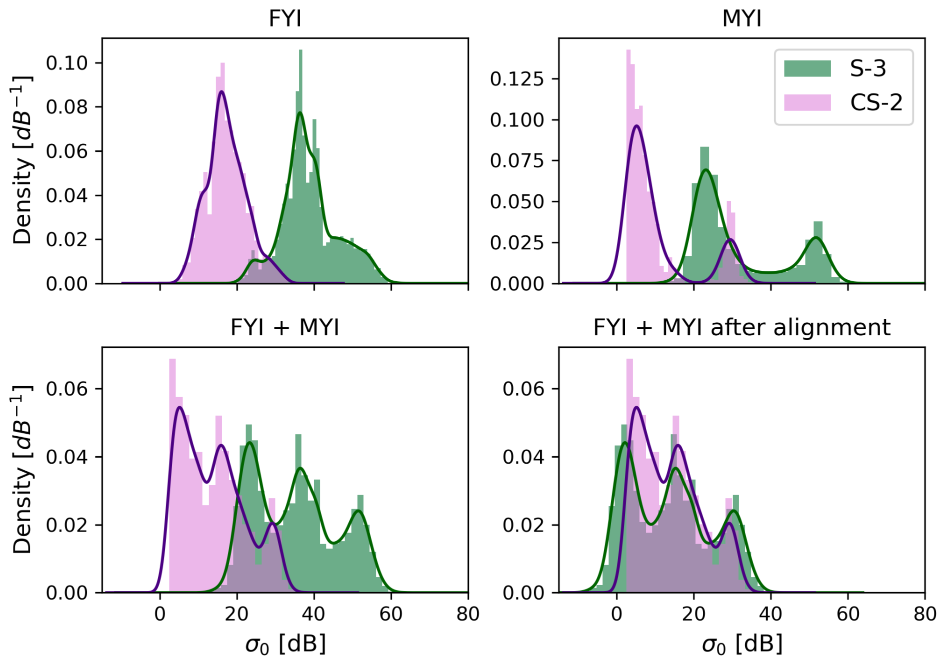
Figure A3 Sigma nought backscatter distributions and kernel density estimates for CS-2 and S-3 per ice type (top row) and for both ice types together, before and after alignment (bottom row).

A3 Calibrating radar backscatter values across the CS-2 and S-3 sensors

The backscatter values obtained with the S-3 sea ice retracker have not been calibrated against backscatter from CS-2 and therefore a significant shift in backscatter is observed between both sensors, as can be seen in Fig. A3. Here, we align the S-3 backscatter values to the CS-2 ones using the 1-D Wasserstein distance in order to quantify the horizontal shift between the two distributions. The Wasserstein distance is calculated as defined in Eq. (A1), where u and v are the 1D empirical probability density distributions from which the cumulative distribution functions U and V are calculated. The Wasserstein distance is calculated using all S-3 and CS-2 backscatter values over the ROIs and is found to be 21.6 dB over FYI, 21.2 dB over MYI, and 21 dB over FYI and MYI ROIs together. As the shift is similar over FYI and MYI, the averaged value of 21 dB is used as correction factor for both ice types and is subtracted from the S-3 backscatter intensities such that they align with the CS-2 intensities. Lastly, the Wasserstein distance was also calculated over a larger area of the Øer Ice Barrier spanning ∼ 230 km × 100 km to verify that the shifts calculated from the ROIs are representative for the wider region. The Wasserstein distance was 20.5 dB for the entire study area and hence we conclude that the 21 dB over the ROIs is representative.

$$\begin{array}{}\text{(A1)}& D_{\mathrm{1}}(u,v)=\underset{-\mathrm{\infty }}{\overset{+\mathrm{\infty }}{\int }}|U-V|\end{array}$$

The backscatter distributions are shown in Fig. A3 per ice type, and for both ice types together before and after alignment. We can see that the MYI distribution is bimodal, while the FYI distribution is unimodal. The left distribution for MYI represent the increased backscatter intensities in the melt season, while the right peak corresponds to the backscatter pre-melt. For FYI the returns of pre-melt and melt are not distinguishable because backscatter values pre-melt change as the newly-formed ice matures and partly fall in the same range of values as after melt. The distribution for FYI and MYI together is simply the combination of the individual distributions and the result is a multimodal distribution where the modes of FYI and MYI pre-and after melt are clearly visible.

A4 IS-2: custom freeboard derivation for increased coverage in lead-sparse areas

We re-processed all IS-2 freeboards using the custom interpolation scheme described in Sect. 4.5.1 to obtain better laser altimetry coverage over the ROIs. We validate the new freeboards and determine the optimal search distance for lead tie points by comparing all sets of beams from intersecting tracks over the fast ice within a time interval of at most 10 d (≃ 240 h). We test lead tie point search distances of 50, 80, 100, and 150 km. In order to gather enough samples, intersections are collected over an area of ∼ 230 km × 100 km spanning across all ROIs in the time period 15 January–15 May 2022, i.e. when the fast ice is stable and relatively immobile. An intersection is defined from beam-to-beam between two tracks, so for example beam 1 from track A is compared to beam 3 from track B in the location where they spatially overlap. Both inter-beam and intra-beam comparisons are considered as intersections, as freeboard is a relative measure and hence systematic inter-beam range biases cancel out. To get a statistical representation of the freeboard distributions at each intersection, all samples along both beams that are within a certain radius of each other are collected. We used search radii of 250, 500, and 1000 m, which led to search results with time lags of 34, 61, 130, 157, or 226 h. The intersection are then quality-filtered by two criteria: (1) the beam-to-beam difference in average small-scale surface roughness (calculated from the width of Gaussian fit on the photon height distribution) should be less than 0.1, and (2) at least 100 freeboard samples should be available per beam to ensure statistical representability. Intersections where the difference in surface roughness between both beams is more than 0.1 might indicate that both beams sampled a different ice surface, e.g. when the intersection covers both FYI and MYI.

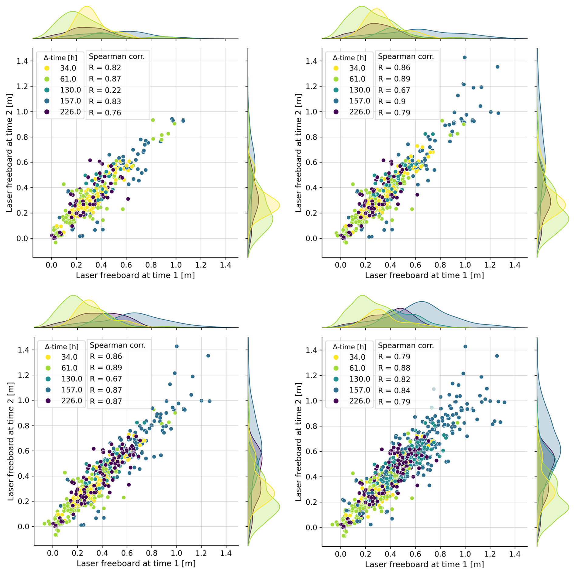
Figure A4 The ICESat-2 cross-over analysis for lead tie point search distances of 50, 80, 100, and 150 km (top left to bottom right). Each plot shows the mean laser freeboards for pairs of intersecting IS-2 beams, color-coded by time lag and with Spearman's correlation coefficient (R) reported per time lag.

Figure A4 shows the scatterplots of laser freeboard pairs for lead tie point search distances of 50, 80, 100, 150 km (top left to bottom right). These plots show that (i) data density increases when increasing the maximal search distance for lead tie points, and (ii) laser freeboards generally show good agreement between overpasses, with correlation coefficients in the range 79–86 for intersections with a time lag of 34 h. The correlation coefficients across the different time lags are stable or even slightly improve for maximal lead tie points distances up to 100 km, but start decreasing for 150 km distance. We concluded that the IDW method with 100 km distance threshold provides reliable sea surface height estimates while maximizing laser altimetry coverage and use this method to obtain a laser freeboard for each ATL07 height sample without corresponding ATL10 freeboard. For the 100 km lead tie point search distance, the number of intersections found at different time lags and search radii is shown in Fig. A5. The absolute difference in laser freeboards at intersections, per time lag and search radius, is shown in Fig. A6. The median absolute difference in laser freeboards is consistently ∼ 5 cm, independently of search radius or time lag, with an exception for the intersections with a time lag of 157 h where slightly higher differences are observed. The variance, however, increases with time lag, especially for the time lags larger than 130 h (∼ 5 d). The higher variance is expected at these time scales, as physical changes are more likely to have happened on the surface.

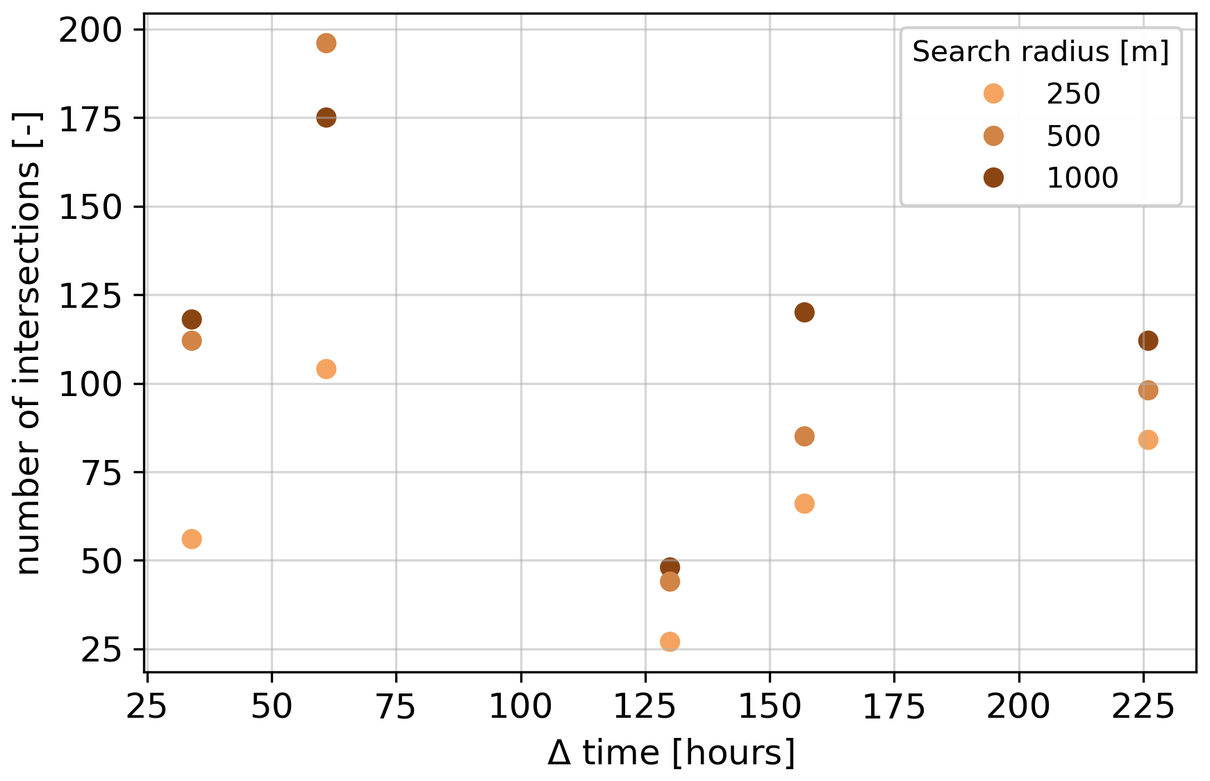
Figure A5 Number of intersections per search radius at five different time lags, for lead tie point search distance 100 km.

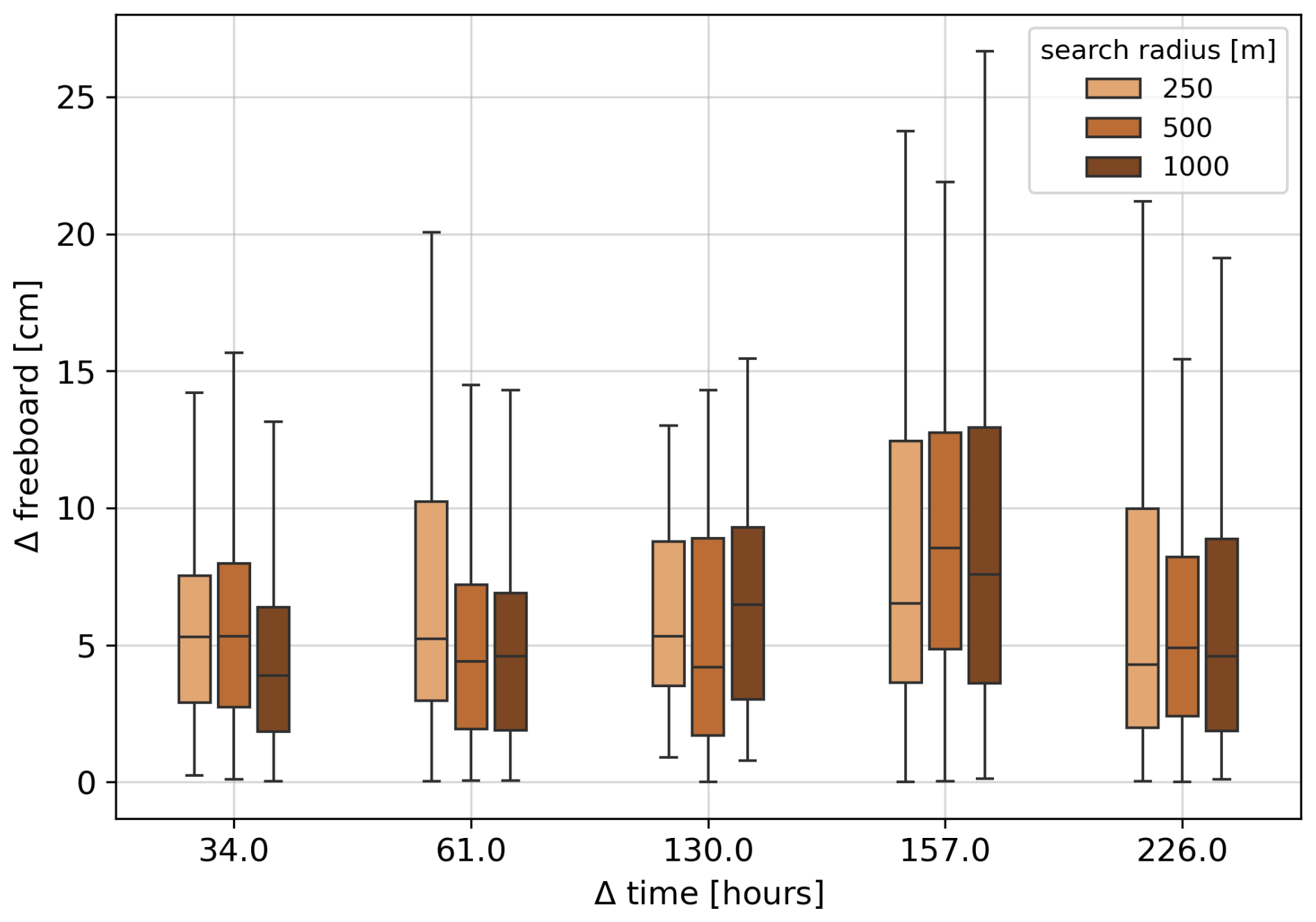
Figure A6 Absolute difference in laser freeboards for all intersections found when using the 100 km search distance for lead tie points, for three different search radii at five different time lags.

Appendix B:  Results

Figure B1 Laser and radar freeboard statistics for FYI and MYI at 15-d intervals.

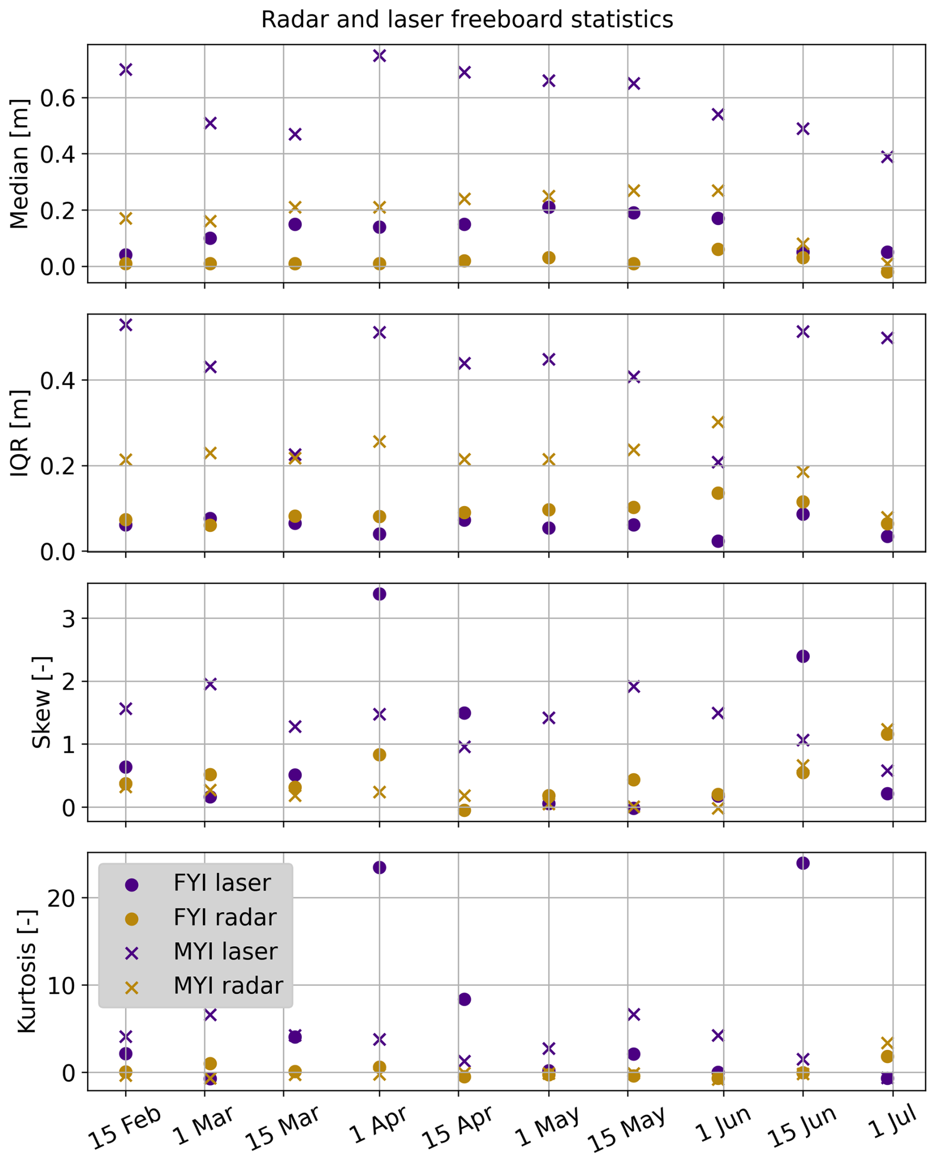
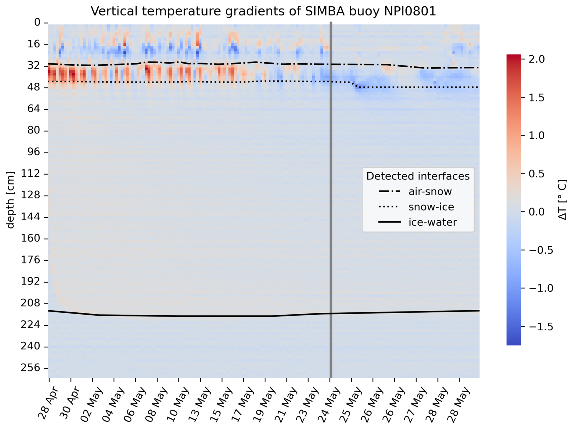
Figure B2 Vertical temperature gradients obtained from SIMBA instrument measurements between 28 April and 29 May 2022. Horizontal lines indicate the air/snow, snow/ice, and ice/water interfaces derived from the heating cycles. The vertical gray line indicates the start of melt onset.

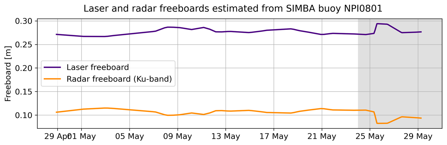
Figure B3 Laser and radar freeboards corresponding to the snow depth and ice thickness time series measured by the SIMBA instrument between 28 April and 29 May 2022. The vertical offset between these laser and radar freeboards and the altimetry-derived freeboards is due to representation issues, as a single SIMBA buoy cannot capture the variability in snow and ice thickness of the highly heterogeneous MYI surface within the ROI polygons.

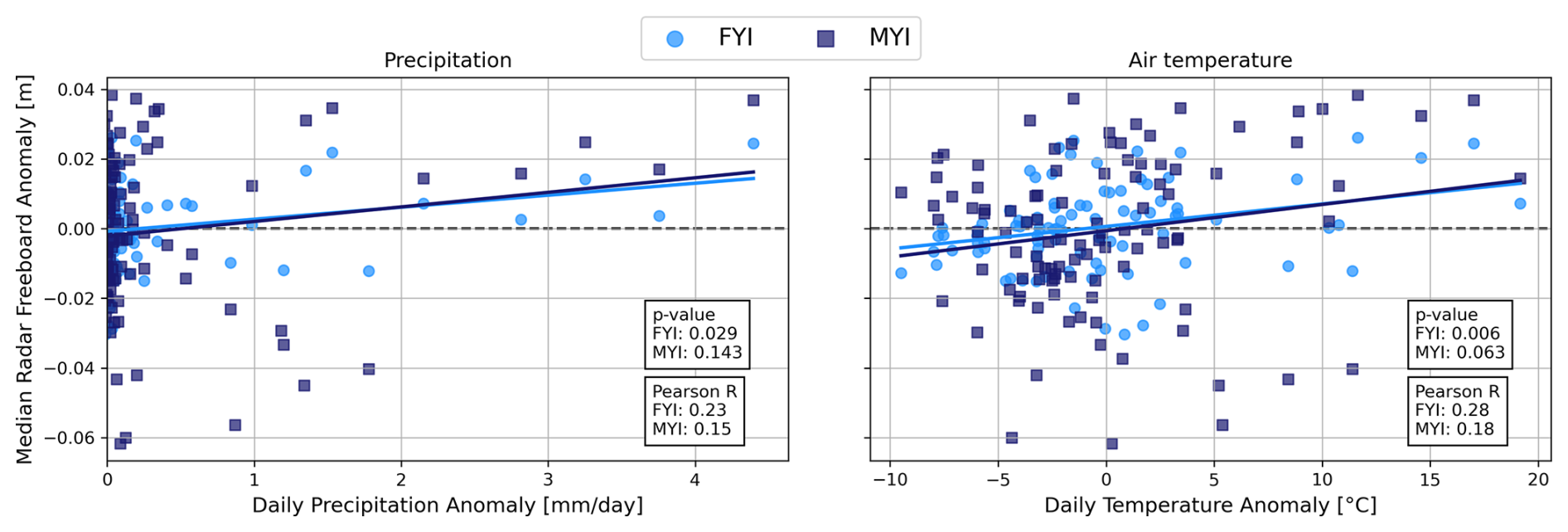
Figure B4 Radar freeboard anomaly versus precipitation anomaly (left) and versus air temperature anomaly (right) during the winter season, per ice type.

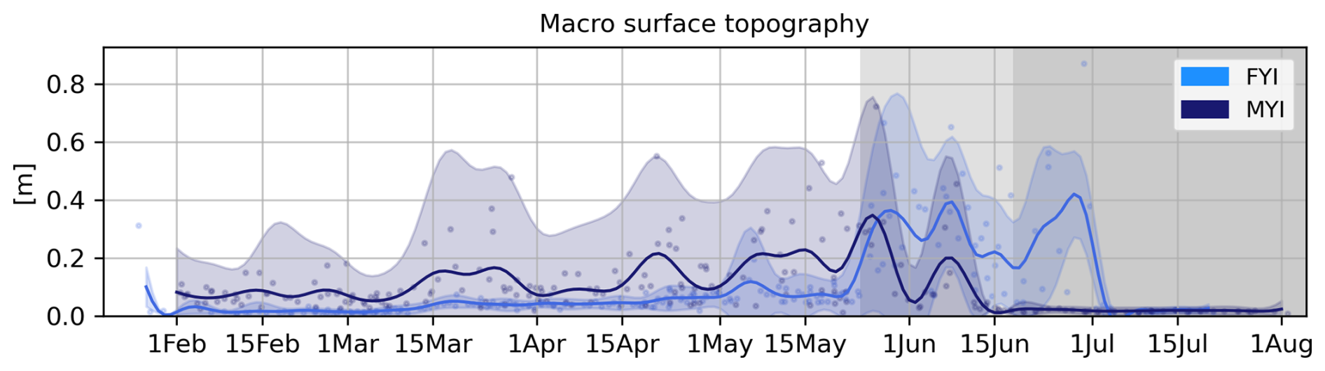
Figure B5 Time series of the effective surface topography root-mean-square height (RMS), one of the four free parameters optimized by the LARM retracker.

B1 Ku-band radar penetration into snow on MYI

We are not able to reliable assess the penetration depth of Ku-band radar waves in the snow cover on MYI. However, the laser freeboard provides an upper bound for the total freeboard (i.e. snow and ice freeboard) and this allows to estimate the minimal penetration depth. In the time series presented here, the average laser freeboard over MYI is 0.6 m while the average radar freeboard is 0.2 m during the winter period. The left schematic in Fig. B6 illustrates these laser (FB_La) and Ku-band radar (FB_Ku) freeboards drawn to scale. The right schematic shows the corresponding snow and ice fractions for the worst case scenario in terms of Ku-band radar penetration, i.e. when the laser freeboard equals the snow depth (SD) and hence the dominant return at Ku-band is at a maximal distance away from the snow/ice interface. Since the MYI in this study is relatively thick, we assume the snow load is not able to cause negative ice freeboards and hence the minimal (FB_i) is zero. The radar freeboard height does not account for delayed radar wave propagation in the snow cover. The corrected freeboard height is obtained through Eq. (8). Since we do not know if this corrected height actually corresponds to the ice freeboard (FB_i), we refer to it as FB_Ku−corr here.

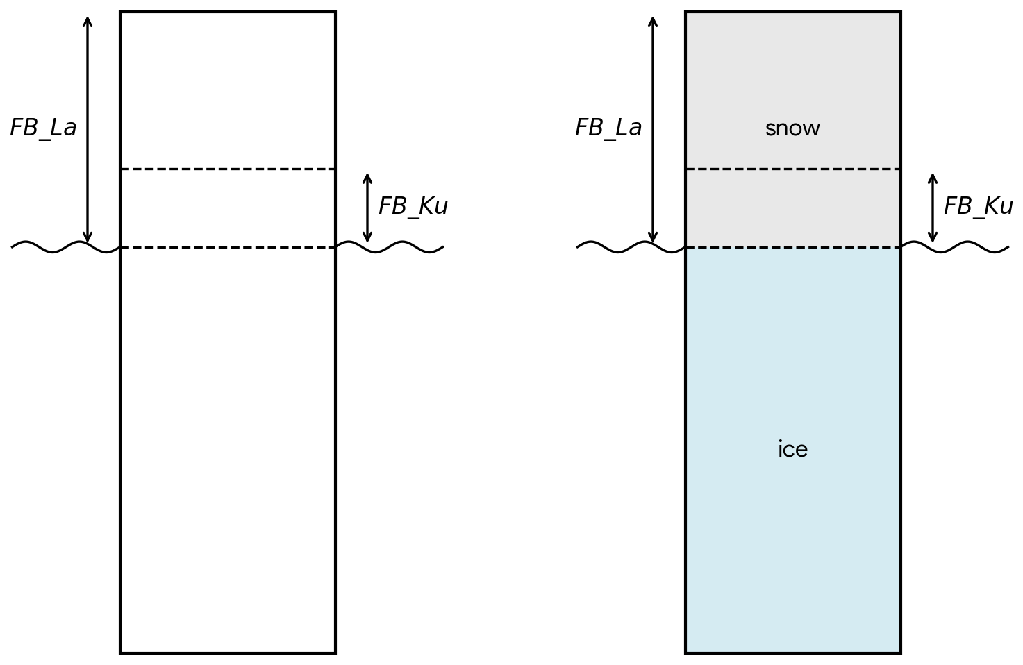
Figure B6 Schematic overview of freeboard estimates obtained from laser (FB_La) and Ku-band radar (FB_Ku) in the context of estimating Ku-band radar penetration depth into snow on MYI. The ratio between laser and radar freeboard height is drawn to scale according to the average heights measured in the winter time series. The right schematic illustrates the worst case scenario, i.e. when the laser freeboard equals the snow depth and the retracked Ku-band return is thus located furthest away from the actual snow/ice interface.

We can summarize the boundary conditions as following:

• FB_La = 0.6 m

• FB_Ku = 0.2 m

• SD ≤ 0.6 m

• FB_i ≥ 0 m

We estimate the minimal radar penetration depth by calculating FB_Ku,corr for the worst case scenario, i.e. when the laser freeboard equals the snow depth (SD = 0.6 m). We use a snow density of 285 kg m⁻³, which is the average snow density over MYI in our time series during the winter period, and obtain:

$${\mathrm{FB}}_{\mathrm{Ku},\mathrm{corr}}\approx \mathrm{0.34}\mathrm{m}.$$

This corresponds to the height above the local sea surface where the main Ku-band radar return is retracked. Therefore, in the worst case scenario, the Ku radar waves only penetrate into the upper 0.26 m of the total 0.6 m snow column, which equals 43 % penetration. We conclude that Ku-band radar waves penetrate at least ∼ 40 % deep into the snow on MYI.