Assessment of Sentinel-3 altimeter performance over Antarctica using high resolution digital elevation models

Since 2016, the Sentinel-3 satellites have provided a continuous record of ice sheet elevation and elevation change. Given the unique, operational nature of the mission, and the planned launch of two additional satellites before the end of this decade, it is important to determine the performance of the altimeter across a range of ice sheet topographic surfaces. Whilst previous studies have assessed elevation accuracy, more detailed investigations of the underlying instrument and processor performance are lacking. This study therefore examines the performance of the Sentinel-3 Synthetic Aperture Radar (SAR) altimeter over the Antarctic Ice Sheet (AIS), utilising new detailed topographic information from the Reference Elevation Model of Antarctica (REMA). Applying Singular Value Decomposition to REMA, we firstly develop new self-consistent Antarctic surface slope and roughness datasets. We then use these datasets to assess altimeter performance across different topographic regimes, targeting a number of key steps in the altimeter processing chain. We also evaluate the impact of topography upon waveform decorrelation. For the new Sentinel-3 Thematic Product, we find that, for 94.1 % of acquisitions, the point of closest approach to the satellite is successfully captured within the range window – an improvement of ∼ 5 % compared to the previous non-thematic (BC-004) product. For both products, performance declines with increasing topographic complexity, which also limits the ability to record all backscattered energy within the beam footprint. We estimate that 57.4 % of the ice sheet exhibits greater topographic variance within the footprint than can be captured by the range window, and that the current window placement captures a median of 89.2 % of the total possible topography that could be recorded. These findings provide a better understanding of the performance of the Sentinel-3 altimeters over ice sheets, and can guide the design and optimisation of future satellite missions such as the Copernicus Polar Ice and Snow Topography Altimeter (CRISTAL) and the Sentinel-3 Next Generation Topography mission.

1 Introduction

From 1992 to 2020, the Antarctic Ice Sheet (AIS) lost a total of 2671 ± 530 billion tonnes of ice (Otosaka et al., 2023), with current rates of ice loss now ∼ 6 times greater than those measured in 1979 (Rignot et al., 2019). Recent studies suggest that this accelerating loss of ice, which has occurred mostly across sectors of West Antarctica and the Antarctic Peninsula, increased global sea levels by 7.4 ± 1.5 mm from 1992 to 2020 (Otosaka et al., 2023). As Earth's climate continues to warm, current projections suggest that the sea level contribution from the AIS will reach multiple decimetres by 2100, with high-end projections exceeding 1 m (Frederikse et al., 2020). This large range in projections, whilst partly due to a variety of forcing pathways, is also linked to uncertainty in the physical processes governing the ice sheet's response to climate change. Within this context, it is imperative to establish and maintain long-term monitoring programmes to better understand the physical processes that control ongoing ice sheet imbalance (Davis et al., 2005; Price et al., 2011; Shepherd et al., 2004). Whilst a range of techniques exist for remote observation of the cryosphere, our understanding of how ice sheets are changing is largely informed by satellite observations, with the longest continuous record coming from the technique of satellite radar altimetry. The principal use of altimetry over ice sheets is to derive estimates of ice sheet elevation and elevation change (Wingham et al., 1998; Shepherd et al., 2019), which, ultimately, can be used to determine ice sheet mass imbalance. Radar altimeters have also been used to investigate a range of other glaciological processes, including grounding line location and migration (Dawson and Bamber, 2017; Konrad et al., 2018; Hogg et al., 2018), subglacial hydrology (Siegfried and Fricker, 2018; Wingham et al., 2006b; McMillan et al., 2013; Gourmelen et al., 2017), ice shelf processes (Griggs and Bamber, 2011; Chuter and Bamber, 2015), and surface mass balance (Slater et al., 2021).

The initiation of continuous ice sheet monitoring by altimetry began with the launch of the ERS-1 mission in the early 1990s, albeit ERS-1 was designed primarily to measure the ocean geoid. Continuity during the following two decades was provided by the ERS-2 and Envisat satellite missions, before the launch of CryoSat-2 (CS2) in 2010, which introduced technical innovations tailored for ice surfaces. Specifically, CS2 pioneered the use of Synthetic Aperture Radar (SAR) altimetry processing and SAR Interferometric (SARIn) altimetry techniques over Earth's cryosphere, delivering substantial improvements in along-track resolution and measurement accuracy, particularly over the complex terrain of the ice sheet margins (McMillan et al., 2014; Gourmelen et al., 2018). Subsequently, Sentinel-3 (S3), which to date comprises two satellites launched in 2016 and 2018, ushered in an era of operational monitoring and global SAR coverage, thus representing another significant milestone in the historical progression of satellite altimetry (Abdalla et al., 2021). The measurements made by radar altimeters over the past 30 years have provided important new insight into the changing nature of Earth's ice sheets. However, like all geodetic techniques, the fidelity of measurements varies, as a consequence of both the instrument design and the complexity of the illuminated ice surface. In the case of radar altimeters, measurement quality typically degrades with increasing topographic complexity, due to the difficulty of keeping track of the ice surface and the failure of assumptions used in Level-2 (L2) processing under such conditions (see Sect. 2 for details).

Whilst a number of previous studies (McMillan et al., 2019; Clerc et al., 2020a; Quartly et al., 2020; McMillan et al., 2021; Aublanc et al., 2025b) have quantified the overall accuracy of elevation measurements derived from the Sentinel-3 altimeter, less attention has been given to investigating the underlying performance of the instrument and, ultimately, how characteristics relating to the instrument and algorithm design have affected the ability of the altimeter to make reliable elevation retrievals. With the recent availability of high resolution Digital Elevation Models (DEMs), such as the Reference Elevation Model of Antarctica (REMA; Howat et al. (2019)), comes the opportunity to evaluate a number of these design choices, and therefore to advance our understanding of altimeter performance. This, in turn, can benefit the design and operation of future altimeter missions. In this study, we therefore use REMA to undertake a detailed evaluation of Sentinel-3 elevation retrievals across the Antarctic Ice Sheet, in order to better understand the impact of topographic characteristics on altimeter performance.

2 Principles of Radar Altimetry

In this section we review the principles governing the acquisition and processing of radar altimeter echoes over ice sheet surfaces, which provides the context for the analysis presented in this study. Radar altimeters work by transmitting a short radio-wave pulse towards Earth's surface and recording the returned echo in the form of a discretised waveform. Each recorded waveform, comprising the sum of incident surface reflections from within the altimeter footprint ordered by arrival time (Brown, 1977), encodes information pertaining to the surface illuminated by the satellite, such as topography, electromagnetic scattering characteristics, and in the case of returns over ocean, wind speed and significant wave height (Quartly et al., 2020). Over uniform surfaces, altimeter waveforms take a distinctive shape, with a clear peak in power, corresponding to the first return from the surface at the point of closest approach (POCA) to the satellite, followed by a gradual decay in the received power – due to the combined influence of the antenna gain pattern and the orientation of the surface relative to the incident radar wave.

For echoes acquired over ice sheet surfaces, however, and in particular in regions close to the ice margins, waveform shape can be more complex, due to numerous discrete regions of backscatter at different elevations and ranges within the illuminated beam-limited footprint, which can combine to create a complex overall waveform structure. Nonetheless, from each recorded echo, an estimate of surface elevation can be derived by measuring the range between the satellite and a fixed point on the leading edge of the waveform, which is assumed to correspond to the POCA return (see Sect. 2.2). This range measurement can then be converted to an estimate of the surface elevation at the POCA, given knowledge of the satellite altitude. Additionally, several other useful descriptive parameters can also be derived from the waveform, including estimates of (1) the ice sheet's backscatter coefficient (σ₀), which can be used to characterise ice sheet properties such as snow depth, grain size, and density (Blarel et al., 2015; Mertikas et al., 2020); (2) the leading edge width, which contains information related to surface roughness and radar wave penetration into the near-surface snow layer; and (3) the trailing edge slope, which is sensitive to both footprint scale topography and subsurface backscattering (Legresy et al., 2005; Rémy and Parouty, 2009).

Commonly, the altimeter antenna footprint width is defined as the point where the beam intensity drops to half-power (−3 dB), which typically corresponds to an approximately circular footprint that is tens of kilometres wide. This is known as the antenna's beam-limited footprint. For conventional, pulse-limited altimeters, however, measurement resolution is typically defined by the pulse duration, which equates to a circular area of ∼ 2 km in diameter, with flat surfaces yielding narrower footprints than rough or sloping terrain. Prior to 2010, altimeters were pulse limited and operated in Low Resolution Mode (LRM), transmitting pulses at relatively low pulse repetition frequency (PRF; ∼ 2 kHz) and performing onboard averaging to suppress radar speckle. While effective over open oceans, LRM faced greater challenges over the cryosphere, due to the relatively large pulse limited footprint, and the lack of information relating to where within the antenna beam footprint the backscattered energy originated from. These limitations motivated a number of the innovations introduced by CryoSat-2, including (1) SAR altimetry processing, which was also used, subsequently, in Sentinel-3, and (2) interferometric SAR (SARIn) altimetry. Each of these innovations is briefly summarised in the following sections.

2.1 Synthetic Aperture Radar

SAR processing addresses the limitations associated with the size of the LRM pulse-limited footprint, by utilising the motion of the satellite to synthesise a larger aperture and, thus, to improve along-track resolution. By transmitting pulse bursts at a much higher PRF (∼ 18 kHz) and using the Doppler effect to discriminate the origin of overlapping pulses based on frequency shifts, so-called “unfocused-SAR” has achieved an improved along-track resolution of ∼ 300 m. Specifically, SAR processing applies a fast Fourier transform to partition received power into multiple “Doppler strips” along-track, thereby improving the resultant resolution. As a given Doppler strip is seen multiple times in the radar footprint, these different looks can be “stacked” to reduce radar speckle through a process of multi-looking. This innovation has enabled smaller-scale features across ice sheets and sea ice to be resolved (Raney, 1998; Tilling et al., 2015).

2.2 Interferometry

Traditional single-antenna altimeters record only echo time delays, constraining surface returns to lie on an iso-range surface at constant distance from the satellite. This creates ambiguity relating to the geographic origin of reflections within the antenna footprint. While SAR processing improves along-track resolution, it cannot resolve this across-track ambiguity.

Interferometric techniques address this by recording phase differences between two spatially separated antennas, enabling the determination of the angle of arrival of backscattered energy in the across-track plane, and thus more precise geolocation of surface echoes. Additionally, interferometric acquisitions enable swath processing, whereby numerous elevation measurements across-track are derived from a single waveform (Gourmelen et al., 2018). CryoSat-2's SARIn capabilities have demonstrated significant improvements over LRM, especially over complex surfaces (Gray et al., 2017; Wang et al., 2019; Aublanc et al., 2021; Wang et al., 2015; McMillan et al., 2018; Chuter and Bamber, 2015), benefiting applications including ice sheet mass balance estimates, grounding line detection and retreat monitoring (Dawson and Bamber, 2017; Hogg et al., 2018), and resolution of small water bodies such as supraglacial lakes (Gray et al., 2017; Ignéczi et al., 2016).

Across most altimetry acquisition and processing chains, there are a number of key processing steps, which ultimately exert a significant control on the resulting accuracy of the retrieved ice sheet elevation measurements. These include onboard tracking by the instrument of the target surface, waveform retracking and echo relocation, and the application of a range of instrument and geophysical corrections. In the following sections, we provide an overview of each of these factors.

2.3 Surface Tracking

In order to capture the backscattered radar pulse that forms each waveform, the altimeter records the incoming energy for a discrete amount of time, corresponding to when it expects the reflection to be received from the surface. Radar altimeters can have a recording window as short as several microseconds, and when this fails to coincide with the surface return then the instrument temporarily loses track of Earth's surface. Therefore, in order to capture returns effectively, an altimeter requires an estimate of the predicted range to the approaching surface. To provide such information, two methods are utilised: “closed-loop” and “open-loop” tracking. Closed-loop tracking predicts the next range based on the history of the last few seconds. Whilst this works well when the range has linear variation, such as over the ocean or the low slope interiors of the ice sheets, its performance degrades over more highly variable terrain, because the range history is a less reliable predictor of the future range evolution. In contrast, open-loop tracking uses information from an a priori Digital Elevation Model (DEM) to provide the satellite with an estimate of the expected range to the ice surface (Donlon et al., 2012a). This method has the potential to more precisely track the complex topography found across many parts of the ice sheet margin. Open loop tracking was first applied onboard the Jason-2 mission, which over land utilised the ESA ACE-1 DEM at 1 km resolution (Birkett and Beckley, 2010). It has subsequently been used by Sentinel-3 during commissioning and ad hoc tasking over land ice surfaces, and is planned to be implemented operationally onboard CRISTAL.

2.4 Retracking

Commonly within L2 processing schema, the leading edge of the waveform is attributed to the POCA on the surface. To extract the associated range measurement, the process of retracking is used, which derives an estimate of the position of the waveform leading edge relative to a specific onboard tracking gate (of known range), often adjusting the tracker range by several meters (Martin et al., 1983; Ridley and Partington, 1988). In general, retracking algorithms can be categorised as “physical” or “empirical”. Physical retrackers fit an analytical model to the received waveform in order to represent the underlying physics of the radar wave's interaction with the scattering surface, whereas empirical retrackers solely consider the geometry of the recorded waveform (Aublanc et al., 2025a; Villadsen et al., 2016; Passaro et al., 2022). In practice, physical retrackers are rarely used over ice sheets, because of their inability to fit irregular waveform shapes caused by complex terrain, and their sensitivity to changes in the scattering properties of the surface (Quartly et al., 2020; Martin et al., 1983; Quartly et al., 2019; Landy et al., 2019; Slater et al., 2019). Conversely, empirical retrackers do not assume waveform shape, and as such, are far more robust to cases where the echo deviates from its theoretical shape. Examples of physical and semi-analytical retrackers include Ice-2 (Legresy et al., 2005), which was applied to low resolution mode ENVISAT data, SAMOSA (Ray et al., 2015), which has been applied to delay-Doppler Cryosat-2 and Sentinel-3 data, and the UCL ice sheet retracker (Wingham et al., 2006a), which is deployed in the Sentinel-3 land ice ground segment. Examples of empirical retrackers include ICE-1, which applies a threshold based upon the OCOG (Offset Centre of Gravity) amplitude (Wingham et al., 1986; Bamber, 1994), and has been used widely since its implementation within the ground segment of ERS-1; the threshold retracker developed by Davis (1997); TFMRA (Threshold First Maximum Re-tracker Algorithm) (Helm et al., 2014); and MultiPeak Ice (MPI), a recent approach designed to handle complex, multi-peaked waveforms (Huang et al., 2024). Within the Sentinel-3 land ice ground segment processing, both the UCL retracker and a threshold OCOG retracker are implemented.

2.5 Slope Correction

As noted in Sect. 2.2, the measured range to the POCA is constrained to lie on an iso-range surface at constant distance from the satellite, leaving its three-dimensional location undetermined. The process of slope correction aims to resolve this ambiguity by identifying the surface origin corresponding to the measured elevation, based on the assumption that the backscattered energy from the point closest to the satellite corresponds to the waveform leading edge. Over rugged terrain, the magnitude of this slope correction can reach tens of meters vertically, and several kilometres across-track, potentially exceeding 100 m for surface slopes of 1° or greater. This makes uncertainties in its application commonly the largest source of uncertainty in non-interferometrically derived elevation measurements (Li et al., 2022; Brenner et al., 2007; Schröder et al., 2017).

Historically, to identify the POCA location, “slope-based” methods were used (Remy et al., 1989; Cooper, 1989; Bamber, 1994; Brenner et al., 1983). These assumed a constant slope within the beam-limited altimeter footprint, which was commonly derived using a priori slope data at nadir (Levinsen et al., 2016; Remy et al., 1989). By assuming an orthogonal reflection from the surface, the approximate location of the POCA can then be determined using trigonometry (Roemer et al., 2007; Brenner et al., 1983). Whilst the assumption of constant slope is reasonable over simpler, homogeneous terrain, the slope method neglects the finer-scale topography within the beam-limited footprint, which may lead to inaccuracies over even moderately undulating areas of the ice sheet (Levinsen et al., 2016). To address this, “point-based” methods were developed which locate the POCA by using a DEM to search for points with minimum range within the beam-limited satellite footprint (Li et al., 2022; Roemer et al., 2007; Levinsen et al., 2016). Such an approach was first introduced by Roemer et al. (2007) using a DEM derived from ERS-1 measurements. Specifically, this approach moves a fixed window the approximate size of the satellite's pulse-limited footprint through DEM data within the beam-limited footprint (Roemer et al., 2007). The POCA location is then identified as the centroid of the window that minimises the mean range between the satellite and the DEM points within that window, with interpolation between DEM nodes used to further improve accuracy and precision. In their initial study, Roemer et al. (2007) found that this new approach outperformed slope-based methods over Lake Vostok within the East Antarctic interior, reducing the error standard deviation from 1.1 to ∼ 0.5 m when compared to ICESat-1 measurements. This was subsequently confirmed over Greenland, both for Envisat (Levinsen et al., 2016) and CryoSat-2 (Li et al., 2022) Low Resolution Mode data. In both cases the dispersion of the elevation differences relative to either airborne or satellite laser altimetry was 2–6 times greater for a slope-based approach in comparison to a point-based approach.

More recently, LEPTA (Leading Edge Point Based), a formulation of a point-based method was proposed by Li et al. (2022), which utilised the ranges spanned by the waveform leading edge to identify the DEM points corresponding to the POCA. The POCA, and consequently the slope correction, was then derived from the mean of the points intersecting the leading edge. This approach has also been generalised to allow retrieval of multiple elevations from a single multi-peaked waveform, which was demonstrated for Sentinel-3 SAR acquisitions (Huang et al., 2024). When benchmarked against ICESat-2, LEPTA achieved a median height difference of < 0.01 m and a median absolute deviation of 0.09 m. However, it remains sensitive to DEM biases and temporal elevation changes due to its reliance on a static DEM (Li et al., 2022; Huang et al., 2024). Finally, AMPLI (Altimeter data Modelling and Processing for Land Ice) (Aublanc et al., 2025a) represents a new facet-based waveform simulation approach to slope correction. When applied to Sentinel-3 UF-SAR (Unfocused Synthetic Aperture Radar) data over the Antarctic ice sheet, the AMPLI method reduced the median elevation bias and median absolute deviation relative to ICESat-2 ATL06 by 18 % and 51 %, respectively, compared to the ESA Sentinel-3 Land Ice Thematic Product, which uses a slope-based approach. In areas with slopes exceeding 0.5°, the corresponding reductions in median bias and median absolute deviation were 83 % and 90 %, respectively.

2.6 Geophysical and Instrumental Corrections

Before use, measurements need to be corrected for both geophysical and instrumental factors. These include accounting for the distance between the antenna and satellite centre of mass, dry and wet troposphere delays, ionospheric delays, and variations in the solid Earth, ocean loading, and polar tide (Quartly et al., 2020). Additionally, ocean tide and inverse barometer corrections need to be applied over floating ice such as ice shelves, the latter of which accounts for changes in atmospheric pressure. Measurements of the satellite range are also impacted by the on-board clock (ultra-stable-oscillator) responsible for measuring the round-trip of the echo (Quartly et al., 2020). Approaches for accounting for these various corrections differ from mission to mission but commonly amount to adjustments of the order of several meters in total. For additional details relating to the corrections applied within the Sentinel-3 ground segment, the reader is referred to the Sentinel-3 SRAL Land User Handbook (Aublanc et al., 2024b).

3 The Sentinel-3 Mission

This study focuses upon the performance of the Sentinel-3 radar altimeter. In this section, we therefore introduce the principal characteristics of the mission.

3.1 Mission and Instrument Overview

The EU's Copernicus programme has overseen the design and production of a significant number of new satellites during the 2010s–2020s. One of these missions, Sentinel-3, has so far launched two satellites, the first of which, Sentinel-3A, launched on 6 February 2016, followed by Sentinel-3B on 25 April 2018. Sentinel-3 was designed, in part, as a successor to the European Space Agency's (ESA) previous altimetry satellites, ERS-1, ERS-2, and Envisat, with the intention of transitioning to an operational programme, and securing a near-continuous ∼ 30 year record of global altimetry data. During the lifetimes of Sentinel-3A and 3B, two further satellite launches are planned, Sentinel-3C and D, in order to sustain an unbroken observational record into the next decade. Sentinel-3 has an orbital period of 101 min such that after 385 complete revolutions (27 d), the ground-track is repeated to within 1 km. This orbital configuration yields a track-to-track spacing of 0.94° longitude at the Equator (Quartly et al., 2020). Both the 3A and 3B satellites orbit with a 98.65° inclination, thus providing coverage between 81.35° S and 81.35° N. The orbit is also configured to maintain a short-repeat sub-cycle, such that after 4 d the mission obtains quasi-global coverage, with a wider ∼ 7° spacing of ground tracks at the equator (Quartly et al., 2020). Driven by its mission objectives, Sentinel-3 operates in a lower-inclination orbit and with a much smaller range window than CryoSat-2, which has an inclination of ∼ 92.03° and uses a SARIn (Synthetic Aperture Interferometric) range window of ∼ 240 m. The lower inclination orbit means that significantly more of the interior of the AIS is missed. However, as Sentinel-3 operates in SAR mode across the entire AIS (unlike CryoSat-2), much of the interior of the ice sheet is for the first time mapped with a higher along-track resolution. Due to the smaller range window of ∼ 60 m (EUMETSAT, 2017), however, it is not uncommon for Sentinel-3 to fail to capture the surface echo, especially across coastal regions of the ice sheet that exhibit complex topography.

During routine operations, Sentinel-3 operates nominally in closed-loop tracking mode across the ice sheets, thus mirroring the approach implemented on many previous altimeters, such as Envisat and CryoSat-2. Although the satellite was equipped with open-loop tracking capabilities from launch, and indeed this was activated during the commissioning phase of Sentinel-3A, subsequent analysis indicated that the Open-Loop Tracking Command (OLTC) tables were not sufficiently precise over the steep Greenland and Antarctica ice sheet margins to satisfactorily track the complex ice surface (SentiWiki, 2025). Recently, however, several target areas have again been acquired with open loop tracking, for the purposes of re-evaluating and improving open loop tracking over ice sheets. Notably, the OLTC tables are now informed by the high resolution REMA and ArcticDEM DEMs, with the aim to overcome the limitations encountered during commissioning.

The primary altimetry instrument on board Sentinel-3, SRAL (Synthetic Aperture Radar Altimeter), is a Ku-band SAR altimeter. Sentinel-3 achieves ∼ 300 m along-track resolution (291–306 m depending on orbit height) and a pulse-limited across-track resolution of ∼ 1.6–2 km, depending upon surface topography and satellite altitude (Donlon et al., 2012a; SentiWiki, 2025). The overall beam-limited footprint, defined by the antenna's 3 dB beamwidth (where antenna power drops to half its peak value), covers approximately 18.2 km across-track (9.1 km either side of the ground track) (Donlon et al., 2012a), representing the maximum illumination width over which targets can contribute significantly to the returned echo. Specifically, SRAL emits patterns of 64 coherent Ku-band pulses in a burst (with a high Pulse Repetition Frequency of 17.825 kHz), surrounded by 2 C-Band pulses (Donlon et al., 2012b), with the received power partitioned into 64 Doppler strips along-track to achieve the ∼ 300 m resolution. Accompanying SRAL, Sentinel-3 also carries a microwave radiometer (MWR), Sea and Land Surface Temperature Radiometer (SLSTR) and an Ocean and Land Colour Imager (OLCI) (Clerc et al., 2020b).

4 Data

The objective of this study is to provide a detailed assessment of the impact of surface topography on the performance of SRAL across the AIS. For the purposes of this study, we therefore analysed one complete cycle of data acquired by both Sentinel-3A and Sentinel-3B. Specifically, we selected cycle 54 for S3A and cycle 35 for S3B, which were acquired over the periods 15 January to 11 February 2020 and 25 January to 22 February 2020, respectively. As our primary dataset, we used the Sentinel-3 Hydro-Cryo Altimetry Thematic Baseline Collection (BC) 005 Land Ice product (S3A_SR_2_LAN_LI and S3B_SR_2_LAN_LI; available at https://dataspace.copernicus.eu/, last access: 27 February 2026). This product builds on the previous, unified BC-004 “Land Product”, with a specific land ice chain that makes up one of three new families of “Thematic Products” (Aublanc et al., 2025b). The BC-005 land ice product includes a number of dedicated ice sheet processing algorithms, the most notable of which involves artificially extending the range dimension of the delay-Doppler stack during Level-1 (L1) range migration and multilooking, in order to better preserve backscattered energy in the final waveform, particularly over the ice sheet margins (Aublanc et al., 2025b, 2018). Further details relating to the thematic product can be found in the Sentinel 3 SRAL Land User Handbook (Aublanc et al., 2024b). Whilst our primary analysis focuses on the latest BC-005 product, for context, we also include selected comparisons to the previous BC-004 product, in order to better understand the impact of changes in key processing steps on retrieval performance across varying surface conditions. These comparisons are specifically designed to provide new insight into how processing changes can affect retrieval quality, with direct relevance for the design of the processors for future missions such as CRISTAL.

In order to investigate the performance of Sentinel-3, we used the 100 m resolution, version 2 REMA (Reference Elevation Model of Antarctica) mosaic (Howat et al., 2022) (available at https://www.pgc.umn.edu/data/rema/, last access: 27 February 2026). REMA is a high-resolution DEM covering nearly 98 % of Antarctica, which has been used for a range of cryospheric applications (Chartrand and Howat, 2020; Zinck et al., 2023; Liu et al., 2023). REMA was created by applying stereophotogrammetric techniques to submeter resolution commercial optical satellite imagery, including data from Maxar, WorldView-1, WorldView-2, and WorldView-3, as well as a small number of acquisitions made by GeoEye-1 (Howat et al., 2019). To form the mosaiced product, individual DEMs were registered to satellite altimetry measurements from CryoSat-2 and ICESat, leading to an estimated absolute uncertainty of less than 1 m, and relative uncertainties of the order of decimeters (Howat et al., 2019). For the purposes of this study, we selected REMA over other DEMs, such as the ICESat-2-derived gridded ATL14 product (Smith et al., 2021), as it is generated from stereoscopic techniques, and thereby provides a high-resolution, inherently two-dimensional product with minimal gaps. In contrast, the ATL14 product includes interpolation between ICESat-2 tracks, particularly as track-to-track spacing increases away from the poles (Smith, 2021), which makes it less well suited to constraining small-scale topographic characteristics, such as footprint-scale surface roughness.

5 Methodology

In this study, our aim is to assess and better understand the performance of the S3 altimeter over a variety of topographic regimes. To achieve this, we firstly use REMA to generate new ice sheet wide estimates of surface slope and roughness. We then performed three different sets of analysis (1) an evaluation of the extent to which the onboard tracker's placement of the range window and subsequent processing maximises the proportion of the illuminated topography that contributes to each waveform (i.e. that is captured by the range window), (2) an assessment of the extent to which the placement of the range window successfully captures the point of closest approach on the illuminated ice surface, and (3) quantification of the degree of correlation between along-track sequences of echoes. The first analysis is designed to provide a first assessment of the effectiveness of the altimeter in adequately tracking the underlying topographic surface. The second analysis is designed to evaluate the assumption – which is inherent to most L2 processing schemes – that the waveform leading edge originates from the closest point within the beam footprint; and then to investigate how the validity of this assumption varies with increasing topographic complexity. The third analysis evaluates the extent to which the complexity of the topographic surface – characterised by slope and roughness – causes decorrelation in successive delay-Doppler echoes. In the following sections, we outline the methodology used for each of these analyses, in turn.

5.1 Ice Sheet Surface Slope and Roughness from REMA

To understand the impact of ice sheet surface topography on the performance of the Sentinel-3 altimeter, we used the REMA dataset to compute continent-wide estimates of ice sheet surface slope and roughness. Within the context of this study, these parameters are important because they can affect (1) the ability of the altimeter to track the ice sheet surface, (2) the effectiveness of approaches to derive the waveform, and (3) the degree of correlation between sequences of waveforms acquired along the satellite track.

We generated our own slope and roughness maps using REMA in order to tailor the algorithms used to fit with the objectives of this study. Although there exist several easy-to-apply methodologies for calculating slope from DEMs (Horn and Schunck, 1981; Zevenbergen and Thorne, 1987), common approaches for calculating roughness such as the Terrain Ruggedness Index (TRI) (Riley et al., 1999), the Topographic Position Index (TPI) and Roughness (Wilson et al., 2007), do not fit our use-case, despite extensive application in GIS (Geographic Information System) programs and packages such as GRASS, ArcGIS, and GDAL (used by QGIS). This is because these methods use the local variance in elevation as a measure of roughness, but neglect to account for topographic slope. Instead, they calculate the differences between a pixel and its immediate neighbours, which would, for example, return a non-zero roughness value over a perfectly smooth plane inclined at an angle. Consequently, the roughness values produced by these methods are dependent on slope, making it difficult to separately assess their individual contributions to topographic variation. More advanced metrics such as the Vector Ruggedness Measure (VRM) (Sappington et al., 2007) attempt to address this through calculating the dispersion of local surface normals, but (1) do not explicitly decouple slope from the roughness calculation, and (2) express roughness as a unitless 0–1 value, which neglects recording useful elevation amplitude information. Additionally, a recently developed approach (Scanlan et al., 2023) applies Radar Statistical Reconnaissance (RSR) to radar altimetry echoes to estimate wavelength-scale roughness over the Greenland ice sheet. However, RSR characterises centimetre-scale surface variability at fundamentally different length-scales than our focus on topographic roughness within the radar altimeter beam footprint (hundreds of meters to kilometres), and requires aggregation of ∼ 1000 echoes per grid cell, limiting spatial resolution to ∼ 5 km. Therefore, to explicitly decouple slope from roughness at the relevant scale, we calculate roughness by quantifying the dispersion of orthogonal residuals from a best-fit plane, implemented using Singular Value Decomposition (SVD), and applied to a DEM over a sliding-window. In addition to eliminating any artificial correlation between slope and roughness that is introduced by other methods, this approach also provides a more accurate measure of slope than commonly used approximations such as Horn's method (Horn and Schunck, 1981) by explicitly fitting a plane, whilst also allowing for flexible window sizes beyond the 3×3 pixel constraint inherent to those approaches. To fit the plane, SVD was chosen, rather than a least-squares (LS) approach, as SVD fits a plane by minimising orthogonal residuals, whereas LS minimises residuals in the vertical (z) direction. This, we believe, makes SVD more suitable for fitting surfaces over complex terrain, where minimising the true geometric (orthogonal) distance is expected to yield a more representative estimate of the surface slope. Furthermore, SVD directly returns the normal vector to the fitted plane during the fitting process, with LS otherwise requiring a separate, additional calculation. For the window size, we used 9×9 pixels (900×900 m), with slope and roughness parameters only computed where more than half of the pixels within a window contained a valid elevation measurement. The window size was chosen to be broadly consistent with the size of the pulse-limited footprint and to minimise the impact of missing data.

To obtain slope and roughness values we first construct a matrix $\mathbf{M}\in {\mathbb{R}}^{n\times \mathrm{3}}$, containing the n mean-centered 100 m resolution REMA coordinates ($x,y,z$) within each window (Eq. 1). We then apply SVD to this matrix, as defined in Eq. (2), which decomposes M into the product of three matrices: an orthogonal matrix U containing the left singular vectors, a diagonal matrix Σ containing the singular values in decreasing order, and an orthogonal matrix V whose columns are the right singular vectors. The right singular vector corresponding to the smallest singular value – i.e., the last row of V^T – defines the unit normal vector $\mathit{n}=[n_x,n_y,n_z]$ of the best-fit plane through the points in the window. The surface slope is then derived from the gradient of the fitted plane, given by the partial derivatives $\frac{\partial z}{\partial x}$ and $\frac{\partial z}{\partial y}$ (Eq. 3), with a final, singular slope value s computed by taking the Euclidean norm of the two directional gradients and converting to degrees. This yields the local surface slope angle, independent of orientation (Eq. 4). Roughness r is calculated as the minimum-to-maximum range of the orthogonal residuals, obtained by taking the dot product of each centered point with the plane normal, where m_i is the ith row of M (Eq. 5). To obtain single slope and roughness values for each record, we then take the mean of the pixel values contained within the corresponding beam-limited footprints.

$$\begin{array}{}\text{(1)}& {\displaystyle }\mathbf{M}=\left[\begin{array}{ccc}{x}_{\mathrm{1}}-\stackrel{\mathrm{‾}}{x}& y_{\mathrm{1}}-\stackrel{\mathrm{‾}}{y}& z_{\mathrm{1}}-\stackrel{\mathrm{‾}}{z}\\ \mathrm{⋮}& \mathrm{⋮}& \mathrm{⋮}\\ x_n-\stackrel{\mathrm{‾}}{x}& y_n-\stackrel{\mathrm{‾}}{y}& z_n-\stackrel{\mathrm{‾}}{z}\end{array}\right]\text{(2)}& {\displaystyle }\mathbf{M}=\mathbf{U}\mathbf{\Sigma }{\mathbf{V}}^T\text{(3)}& {\displaystyle }a=-{\displaystyle \frac{n_x}{n_z}},b=-{\displaystyle \frac{n_y}{n_z}}\text{(4)}& {\displaystyle }s=\arctan \left(\sqrt{a^{\mathrm{2}}+b^{\mathrm{2}}}\right)\cdot \left({\displaystyle \frac{\mathrm{180}}{\mathit{\pi }}}\right)\text{(5)}& {\displaystyle }r=\underset{i}{max}({\mathbf{m}}_i\cdot \mathbf{n})-\underset{i}{min}({\mathbf{m}}_i\cdot \mathbf{n})\end{array}$$

To facilitate comparison with established methods, we also generate a slope map using Horn's method (Horn and Schunck, 1981), applied to the same 100 m resolution REMA dataset. Since Horn's method uses a 3×3 pixel window (300×300 m), we re-compute our slope map using the same window size for a fair comparison. Similarly, we compute roughness maps using TRI and our method, again using a 3×3 pixel window to ensure consistency with TRI (see Sect. 6.1.2 and Fig. 4). Here, TRI was chosen over alternatives such as TPI and Roughness due to its more extensive prior application in terrain analysis (Trevisani et al., 2023).

5.2 Window Placement Optimisation

Prior to performing a detailed assessment of the range window placement relative to the point of closest approach (Sect. 5.3), we first investigated more broadly the extent to which the placement of the range window maximises the capture of the topographic surface illuminated by the beam-limited footprint. Our motivation for this analysis is grounded on the principle that maximising the amount of information captured is beneficial for a range of present and future use cases. Specifically, whilst it is clear that current non-interferometric processing methods largely rely on information extracted from the leading edge of the waveform, it is likely that future advances in retrieval algorithms may allow full-waveform retrievals. Thus, there is benefit to assessing how the size and placement of the range window can be optimised in order to capture as much of the illuminated surface as possible.

To perform this analysis in practice, for each echo within our chosen cycles (comprising a total of 8 125 872 records), we computed the proportion of DEM points within the beam-limited footprint that fell above, within and below the ∼ 60 m range window, where the beam-limited footprint was defined with dimensions of 18 200 and 300 m in the across and along-track directions, respectively.

Because over complex topography, the range of elevations within the beam-limited footprint exceeds that spanned by the range window, it is, in places, impossible for the range window to entirely capture the illuminated topographic surface. To account for this, we therefore also computed the hypothetical positioning of the range window that would have maximised the capture of topography, together with the associated percentage of the illuminated surface that could be captured within it. This was done by iteratively moving the range window by 1 m increments in range, to determine the position that maximised topographic capture. Having located the optimal range window placement, we were then able to quantify the possible increase in the proportion of the surface captured, which could be realised with a refined range window placement, whilst respecting the inherent limitations imposed by the 60 m range window size. This was assessed by computing the ratio of actual to maximal topographic capture. Finally, we also computed the optimal range window position – and thus the maximum possible topographic capture – that could be achieved for varying-sized range windows; specifically: 60, 120, 180, 300, and 360 m. This allowed us to explore the extent to which an increased range window size would, in principle, yield greater capture of the illuminated topographic surface, with a view to improving our broader understanding within the context of other current and future satellite altimetry missions overflying Antarctica.

5.3 Capture of the Point of Closest Approach

Following the methodology presented in Sect. 5.2, we also performed a similar assessment, which focused specifically on evaluating the window position relative to the point of closest approach. This is motivated by the fact that, within conventional L2 altimetry processing chains, an assumption is made that the echoing point (the so-called POCA) lies within the intersection of the range window and the beam-limited footprint (class 2 in Fig. 1); and thus that the return from the POCA location corresponds to the range to the waveform leading edge. However, around the complex topography of the ice sheet margin, this assumption does not always hold, particularly for Sentinel-3, due to its relatively small (∼ 60 m) range window. In regions of high slope, the POCA may lie outside the beam-limited footprint, meaning that any backscattered energy will be highly attenuated by the antenna gain pattern, whereas in regions of rugged (highly variable) topography, the POCA may lie at an elevation not captured by the range window. With the availability of new, high-resolution DEMs such as REMA, comes the opportunity to explicitly assess the extent to which the echoing point lies within the intersection of the beam-limited footprint and the range window, and hence the extent to which this common assumption in L2 processing chains is satisfied. Furthermore, by comparing success and failure at the ice sheet scale to covariates such as surface roughness and slope, we aim to assess how performance is affected by topographic complexity. For all S3A and S3B echoes within our chosen cycles, we therefore classified where the identified POCA location lay relative to the positioning of the S3 range window. The acquisition geometry and related definition of the POCA classes are shown in Fig. 1.

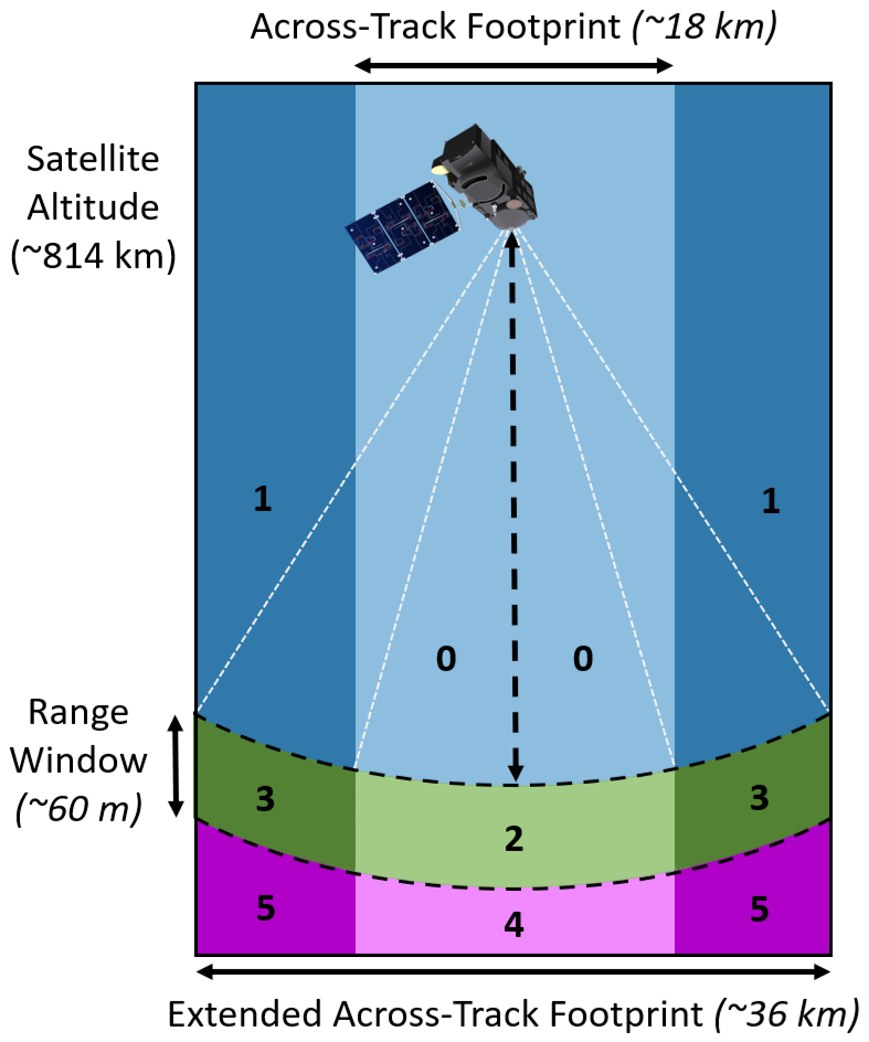
Figure 1 Illustration of the Sentinel-3 SAR altimetry acquisition geometry in the across-track plane (satellite flying into the page), showing the classification scheme used to categorise each acquisition according to the location of the POCA relative to the positioning of the range window. Above the range window is shaded in blue (classes 0, 1), below in magenta (classes 3, 4), and within the range window in green (classes 2, 3). Darker shades of each colour represent locations outside of the across-track beamwidth.

Within this assessment, we performed two sets of analyses. First, we evaluated the positioning of the range window relative to the POCA location that was defined within the standard L2 product. Here, slope correction – and consequently the determination of the location of the POCA within the SAR footprint – is performed via a slope-based approach using a surface slope model precomputed from DEMs over Antarctica and Greenland (Helm et al., 2014; Aublanc et al., 2024b; IPF Team, 2024). This analysis allows us to determine the extent to which the slope correction applied within the L2 processing chain identifies an echoing point that is consistent with the actual acquisition geometry (i.e. lies within both the beam-limited footprint and the range window); in other words, whether the subsequent elevation measurement derived by retracking the waveform can reasonably be attributed to the assigned POCA location. Secondly, we performed the same evaluation, but for a POCA location that we determined, independently, by minimising the range between the ice surface and the altimeter, using the REMA DEM. This procedure follows the point-based relocation method introduced by Roemer et al. (2007), but extends the search region beyond the nominal across-track 3 dB antenna footprint of 18.2 km (Donlon et al., 2012a). We use an extended across-track region of ∼ 36 km (approximately double the 3 dB beamwidth) to identify instances where the POCA lies outside, but proximal to, the 3 dB footprint, where there will still be some limited sensitivity to backscattering from this location (Fig. 1). We refer to the identified surface location as the REMA-derived POCA. It is important to note that although the underlying algorithm is similar, the purpose of this analysis is not to perform a slope correction (i.e. the intention is not to derive relocated elevation measurements as part of a standard L2 processing chain). Rather it is simply to determine the location of the closest surface point to the satellite (as determined by REMA), thereby allowing us to identify the extent to which the positioned range window captures this POCA location.

To perform these analyses, we first located the range window relative to the ice surface for each of the ∼ 8 million altimeter records considered in this study, and then compared it to the two POCA locations. Specifically, we adjusted the range to the nominal tracking point (defined for S3 as the 43rd bin in the range window) according to the geophysical and instrument corrections supplied within the product, to account for path delays due to dry tropospheric, wet tropospheric and ionospheric effects; tidal and atmospheric pressure induced variations, and the instrument Centre of Gravity (COG) correction. As all of these corrections are supplied at 1 Hz,we used linear interpolation to match these to the native 20 Hz frequency of the range and elevation measurements. Finally, the dimension of the range window (128 bins) was used to locate the range to the start and end of the window for each record. To reference the range window to the DEM elevation, we then subtracted the satellite altitude.

Next, we computed the geographic coordinates and elevation of the POCA for both the L2 and REMA derivations, in order to classify them according to their position relative to the range window (Fig. 1). For the L2 evaluation, the geographic coordinates (x,y) were simply taken from the product. For the surface elevation (z) at the L2 POCA, we chose to extract the elevation at this location from the closest REMA pixel, rather than use the elevation within the altimeter product, because the purpose was simply to compare the range window to a reference surface, rather than interpret the altimeter elevation itself. This approach therefore avoided missing data in the L2 product. We selected the nearest REMA point, rather than applying a more complex interpolation method, as the 100 m posting is already finer than the altimeter resolution (∼ 1600×300 m). In this regard, our aim is a coarse-scale classification of the POCA location relative to the range window, rather than the derivation of relocated elevation measurements themselves, and so a more detailed interpolation was unnecessary. For the REMA derivation of the POCA, we computed the echoing point location based upon the DEM pixel that minimised the range between the satellite and the ice surface.

5.4 Along-track Decorrelation of Echoes

Finally, we explore the extent to which ice sheet surface topography causes decorrelation in sequences of SAR waveforms, as they are acquired along the satellite track. This analysis extends the work of McMillan et al. (2021), to investigate the rate at which waveforms decorrelate in space (along-track), and the extent to which this is governed by the topographic characteristics (slope and roughness) of the surface. More specifically, we calculate (1) correlations between adjacent pairs of waveforms aligned in range, and (2) correlations between every waveform and the 50 subsequent waveforms along-track (spanning a distance of ∼ 15 km), also aligned in range. The latter assessment allows us to quantify the rate at which waveforms decorrelate in space, spanning distances that are representative of those over which altimetry measurements are commonly aggregated; for example, when computing rates of surface elevation change, which typically combine elevation measurements over length scales of the order of 10 km. We therefore chose 15 km as indicative of this length scale. Whilst we acknowledge that it would be possible to compute decorrelation over different length scales, our aim here is to provide an initial high-level assessment at an indicative length scale, in order to quantitatively test and characterise the conceptual understanding that waveforms become increasingly decorrelated as footprint scale topographic complexity increases. At a practical level, understanding this relationship is of interest, as decorrelation characteristics may influence the effectiveness of combining information from waveforms acquired over different spatial scales. For example, surfaces with greater slope or roughness may induce more variability between nearby waveforms, which may complicate the aggregation of elevations derived from spatially distributed waveforms. Ultimately, by examining these relationships, we aim to provide initial insights into how surface morphology impacts waveform structure, which can help to inform future work towards improved strategies for processing SAR altimetry data in areas of complex topography.

To determine the correlation between any two waveforms, we first normalise the power of each to be between 0 and 1. To avoid cases where a given waveform was excessively noisy, correlations were not computed when the mean power did not exceed the estimated thermal noise by more than 0.15, with thermal noise computed as the mean of the 6 lowest-value waveform samples (Helm et al., 2014; McMillan et al., 2019). Next, we aligned both waveforms according to their centres of gravity (COG) according to Eq. (6), where N is the number of waveform bins (128), and P_n is the power at bin n. Following this, we retained only the overlapping region of the two waveforms, removing any bins that did not intersect.

In order to focus on correlating the principal surface response, rather than peripheral signals and waveform noise, we masked the aligned waveforms by removing peripheral bins from each side of the range window, until a bin with power above 0.15 (chosen for consistency with the previous noise detection) was found in either waveform. If the clipped waveforms had at least 16 bins remaining, we then computed the Pearson correlation coefficient using the pairs of normalised waveform samples. A minimum threshold of 16 bins was chosen as a reasonable lower bound for what constitutes a valid response, based upon an assessment of the waveforms that passed the L2 ice quality checks, which retained a mean COG width of 27.1 bins and standard deviation of 10.2.

$$\begin{array}{}\text{(6)}& \mathrm{COG}={\displaystyle \frac{{\sum }_{n=\mathrm{1}}^{N}n{P}_n^{\mathrm{2}}}{{\sum }_{n=\mathrm{1}}^N{P}_n^{\mathrm{2}}}}\end{array}$$

Next, for each waveform, we computed its Pearson correlation with each of the subsequent 50 waveforms along-track, yielding a series of correlation values relative to the initial waveform. If more than 25 correlation values were available, we fitted a linear regression to estimate the rate of change in correlation as a function of along-track distance. To ensure comparability between all regressions, we explicitly included a correlation value of 1 at d=0, representing the waveform's self-correlation, and constrained the regression to pass through this point, such that the fitted line followed Eq. (7), where d is the number of records along-track, R(d) is the Pearson correlation coefficient, and m is the along-track rate of change in correlation, per 20 Hz measurement. This slope captures the linear decay in correlation from the initial waveform to increasingly distant waveforms along-track, computed over 50 subsequent records (∼ 15 km).

$$\begin{array}{}\text{(7)}& R\left(d\right)=\mathrm{1}+m\cdot d\end{array}$$

Using the fitted slope, we computed the change in correlation at record 50. This provides a more stable estimate of the change in waveform correlation after 15 km, which is not solely dependent upon the initial and 50th records. Based on this approach, a value of 0 indicates that waveforms 15 km away are perfectly correlated, whilst a value of −1 corresponds to waveforms that are fully decorrelated (R=0) after 15 km. Values less than −1 indicate that waveforms are anti-correlated after 15 km; i.e. an increase in power in one waveform corresponds to a decrease in power in the other. This is likely to reflect limitations in the COG alignment of complex waveforms (e.g. correlating a single peak with a double peak waveform) and so we focus our analysis on correlation values between −1 and 0.

To analyse the effect of surface topography on these metrics, we then derived estimates of across-track surface slope and roughness for a 1-D across-track profile approximating the beam footprint of each record, using a 2-D version of the SVD approach described in Sect. 5.1. We intentionally focused this assessment of waveform similarity on across track slope and roughness, because the anisotropic shape of the delay-Doppler footprint means that these parameters in the across-track direction are most likely to have the largest influence on waveform shape.

6 Results

6.1 Ice Sheet Slope and Roughness from REMA

6.1.1 Slope and Roughness Characteristics

First, we analysed the surface slope and roughness characteristics of the Antarctic Ice Sheet, based upon our newly-derived REMA datasets (Fig. 2). Our new surface slope map shows well-established patterns of very low (< 0.1°) surface slope at the ice divides and the floating ice shelves, with steeper slopes prevailing towards the grounded ice sheet margin. Overall, we find that 76.9 % and 89.1 % of the ice sheet have a surface slope below 0.5 and 1.0°, respectively. Turning to ice sheet surface roughness, we find that 62.4 % and 76.1 % of the ice sheet have a surface roughness below 0.5 and 1.0 m, respectively, with lower roughness persisting mostly within the interior of the ice sheet. Of particular note are the clear signatures of mega dune fields in East Antarctica, which typically have roughness of the order of ∼ 1 m and the patterns associated with ice flow across the Ross and Filchner-Ronne Ice Shelves. In broad terms, the interior of West Antarctica is rougher than East Antarctica and, as with surface slope, there is a general trend to increasing roughness towards the ice margin, with surface roughness often reaching several meters close to the coast.

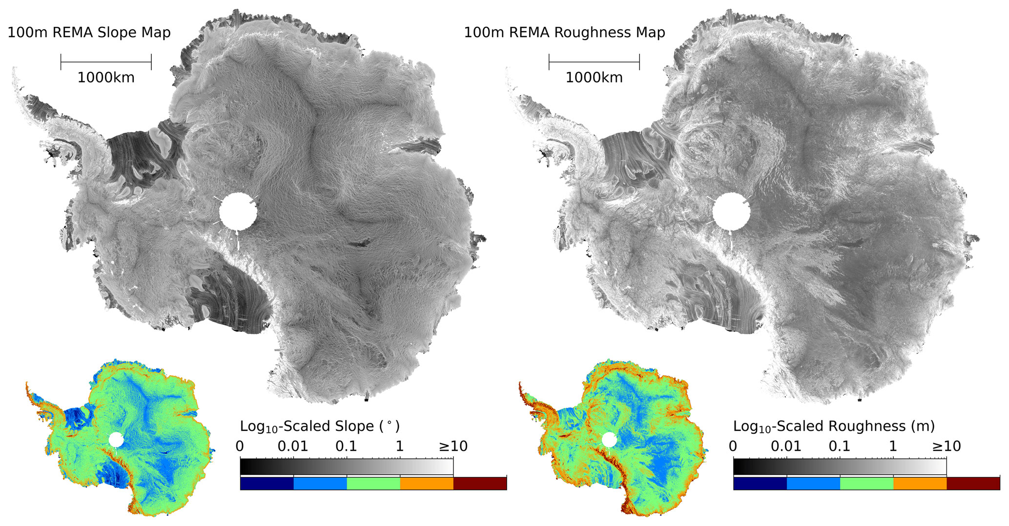
Figure 2 5 km resolution, log₁₀-scaled slope and roughness maps of Antarctica generated using 100 m resolution REMA and the Singular Value Decomposition techniques outlined in Sect. 5.1. The coloured inset maps show discretely binned versions of these datasets, to aid the visualisation of broader scale patterns.

We find that the ice sheet as a whole has a median slope and roughness of 0.192° and of 0.297 m, respectively. We characterise the degree of spatial variability of each parameter across the ice sheet by computing the median absolute deviation, which is 0.134° and 0.219 m for slope and roughness, respectively. To explore in more detail the relationship between surface slope and roughness, we plot their joint and marginal distributions (Fig. 3), which shows a positive relationship between the two variables. Taking the Pearson correlation coefficient, we obtain a value of 0.808, indicating that the two values are significantly linearly correlated. Because we have calculated roughness via the dispersion of orthogonal residuals to the fitted slope, the two variables remain algorithmically independent. Therefore, this correlation reflects a physical relationship between these topographic glaciological parameters, indicating that areas with higher surface slope are also more likely to exhibit higher surface roughness. Broadly, we find that roughness increases by ∼ 4.38 m per degree increase in surface slope.

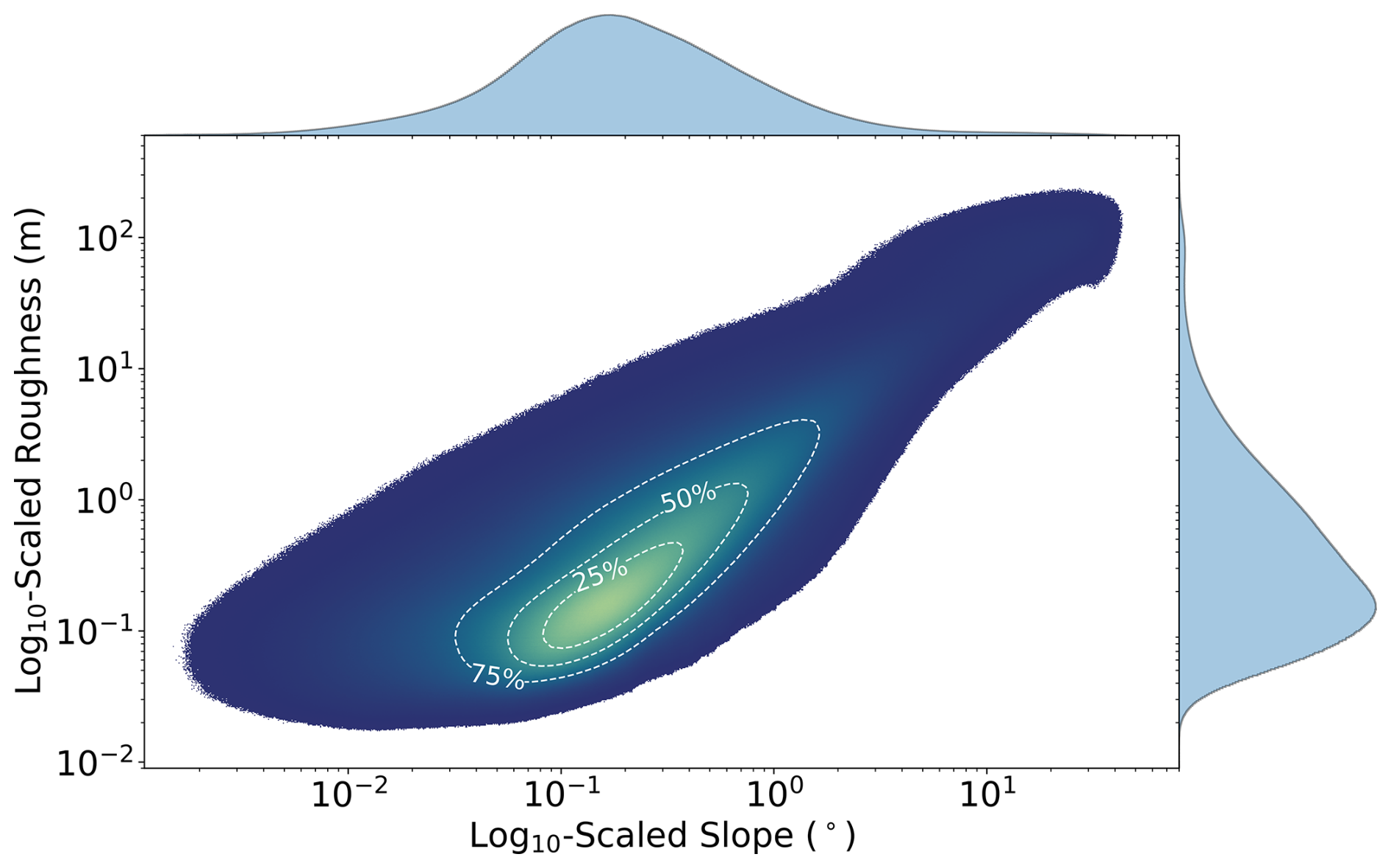
Figure 3 Log₁₀-binned joint and marginal distributions of slope and roughness across Antarctica. The joint distribution is displayed as a density plot, with lighter colours indicating a higher density of measurements, and the contours bounding 25 %, 50 %, and 75 % of the data.

6.1.2 Method Comparison and Validation

As outlined in Sect. 5.1, we also compare our slope estimates to those calculated using Horn's method (Horn and Schunck, 1981). This comparison includes both the slope map shown in Fig. 3, which was generated using a 9×9 pixel window, and an alternative version that used a window size of 3×3 pixels (300×300 m) to match the window dimensions of Horn's method (Fig. 4a). The three results show very close agreement, all attaining the same Gaussian shape on a log₁₀ scale. Specifically, the slope maps derived using Horn's method and our SVD-based approach (both with 3×3 pixel windows) yield median values of 0.199 and 0.198°, respectively, and identical median absolute deviations of 0.138°. The difference between our 3×3 and 9×9 pixel implementations is also negligible (median difference < 0.01°). These results indicate that, when assessed at the scale of the entire ice sheet, and at a resolution of 100 m, neither the choice of window size (3×3 versus 9×9) nor the underlying slope estimation method has a significant impact. It is important to note, however, that the SVD approach is more flexible in offering a generalised solution that can be applied to variable and irregular window shapes, making it better suited for cases where a super-resolution DEM is used, or where slope is estimated over an anisotropic area, such as the 1-D window geometry utilised in Sect. 5.4.

Secondly, we performed a similar analysis for our SVD-derived roughness map (calculated using 3×3 pixel windows), comparing it with estimates made using a 9×9 pixel window, and using the Terrain Ruggedness Index (TRI) approach (Riley et al., 1999) (Fig. 4b). Our method yields a median roughness of 0.03 m and a median absolute deviation of 0.0181 m for a 3×3 pixel window, and a median roughness of 0.297 m and median absolute deviation of 0.219 m for a 9×9 pixel window. For TRI, the corresponding values are 0.864 and 0.592 m, respectively, indicating that our method produces consistently lower roughness values than TRI for both window sizes. The higher values produced by TRI likely reflect its dependency between slope and roughness, whereby steeper slopes inflate roughness estimates. To assess this, we computed the Pearson correlation coefficient between slope and roughness for both methods. We find a stronger correlation for TRI (0.947) than for our approach using the same 3×3 window (0.720). This difference is consistent with TRI not explicitly removing the slope component from its roughness calculation – even a perfectly smooth inclined plane yields non-zero TRI roughness estimates that increase with surface gradient. In contrast, our method decouples these parameters by fitting residuals orthogonal to the best-fit plane. The lower correlation in our method therefore suggests reduced artificially introduced algorithmic correlation between slope and roughness, with the remaining correlation likely reflecting the physical tendency for steeper terrain to exhibit higher surface variability orthogonal to the surface slope.

Turning next to the choice of window size, we find that unlike for slope, the choice of window size has a substantial effect on roughness estimates, with the 3×3 window producing lower values than the 9×9 window (Fig. 4). This likely reflects the fact that an increased number of points in a larger window raises the likelihood of higher minimum-to-maximum variance relative to the fitted plane. Nonetheless, even with a 9×9 window, the distribution of roughness values is still lower for our method than for TRI. Finally, within the context of this study, it is important to note that it is primarily the variance in roughness that is analysed (through comparison to altimetry measurements) rather than the absolute roughness values themselves.

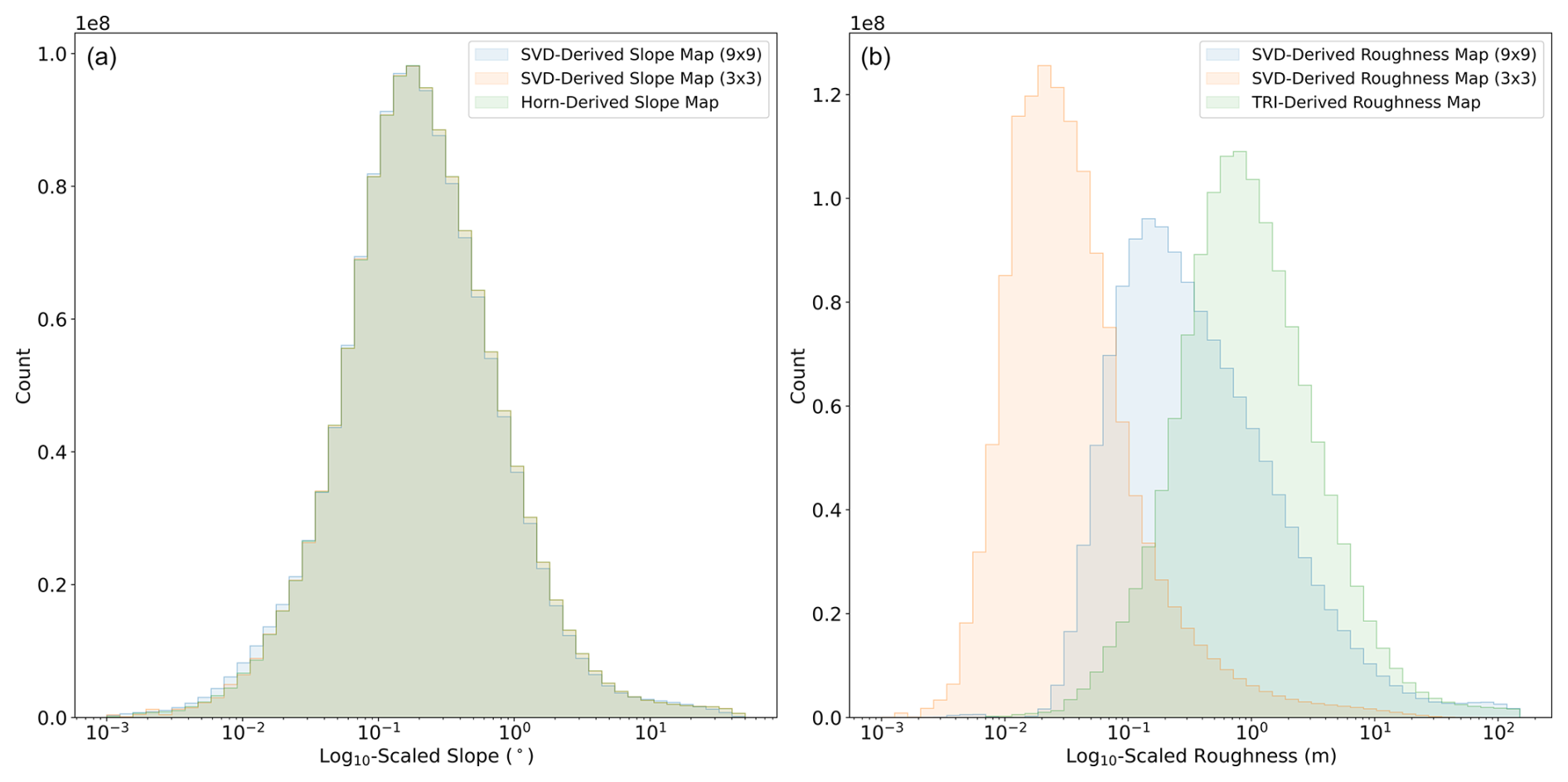
Figure 4 Comparison of slope and roughness estimates using different methods applied to the 100 m resolution REMA DEM. Panel (a) shows slope calculated using (1) Horn's method with a 3×3 pixel (300×300 m) window, (2) our SVD-based approach, calculated with a 3×3 pixel window for consistency with Horn's method, and (3) our SVD-based approach with a 9×9 pixel window. Panel (b) shows roughness computed using (1) TRI (3×3 pixel window), (2) our SVD-based approach using the same 3×3 pixel window size for consistency with TRI, and (3) our approach using a 9×9 pixel window.

6.2 Window Placement Optimisation

6.2.1 Topographic Capture Performance

The S3 product records backscattered energy over a range window of ∼ 60 m. As such, there are areas of the AIS where the degree of topographic variance within the beam-limited footprint makes capturing the full topography within the range window impossible. Determining the locations and extent of these regions is of interest because it indicates where (1) waveforms are likely to be truncated or highly complex, (2) relocation errors may be prevalent, and (3) positioning of the range window will, ultimately, have a major impact upon the reliability of retrievals of ice sheet elevation. By assessing the proportion of illuminated terrain that could be captured with an optimal placement of the 60 m range window (Sect. 5.2), we found that, for 57.4 % of recorded echoes, full (100 %) topographic capture was impossible. With optimal window placement, however, 83.5 % of acquisitions would be able to acquire at least 80 % of the topography illuminated by the beam-limited footprint. Failure to capture the full topography primarily occurs in coastal regions of the ice sheet with high topographic complexity (Fig. 5a), and reflects a fundamental limit imposed by the 60 m size of the Sentinel-3 range window, rather than the onboard tracker implementation.

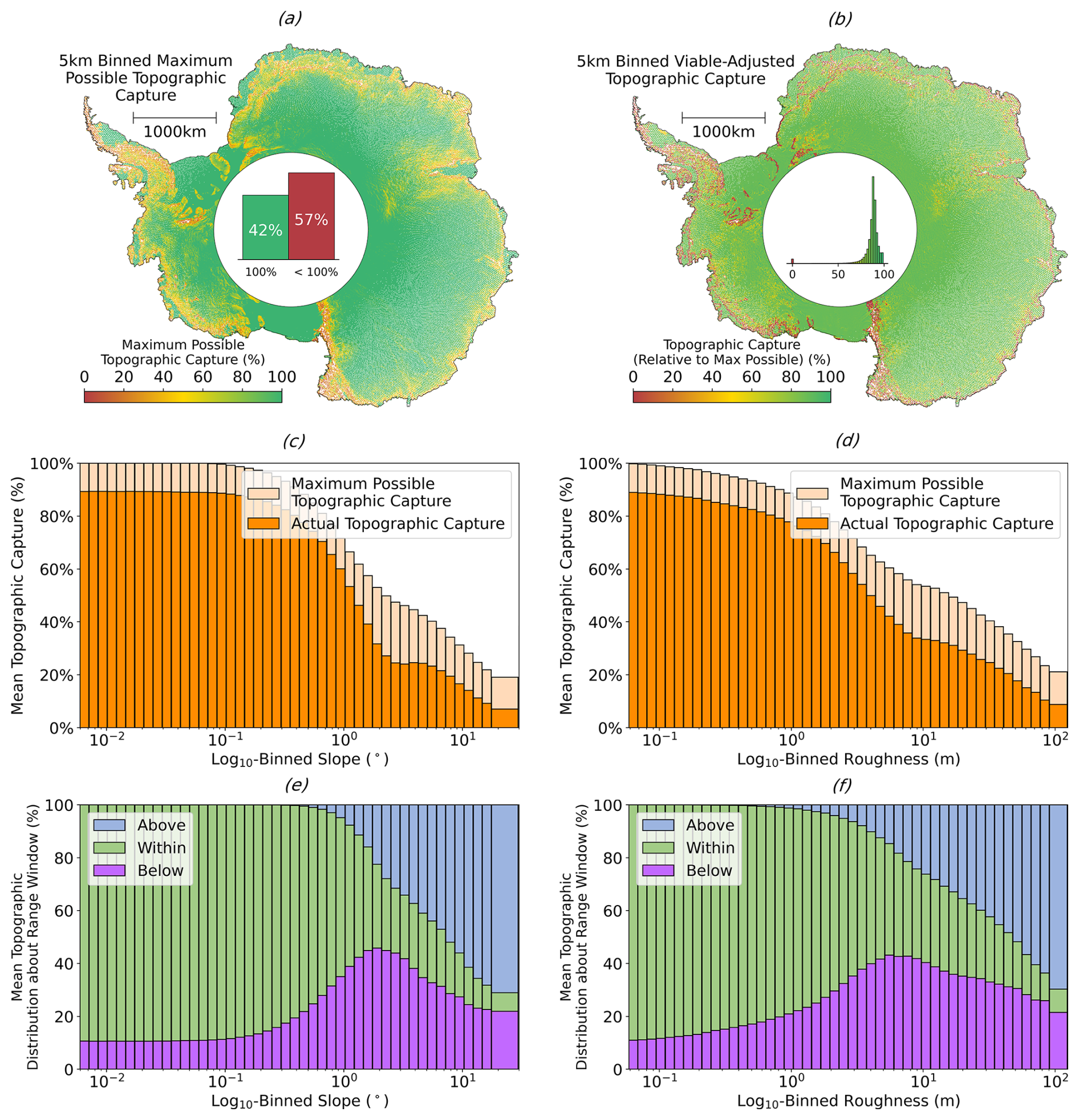
Figure 5 Assessment of the ability of the Sentinel-3 range window to capture the full topographic surface within the beam-limited footprint. Panel (a) exhibits the maximum possible percentage of topography (REMA; 100 m resolution) that can be captured with an optimal placement of the 60 m range window, binned to 5 km. The percentage of records where full (100 %) topographic capture is, and is not, possible is shown within the bar graph in the pole hole. Panel (b) shows the percentage of topography that is captured by the current placement of the range window with respect to the maximum possible capture (panel a), binned to 5 km, with the corresponding distribution shown within the pole hole. A value of 0 indicates that the current placement of the range window entirely misses the ice surface, whereas a value of 100 indicates that the range window captures the maximum possible area of the illuminated surface (not necessarily 100 % of the surface). Panels (c) and d show stacked bar charts representing the maximum percentage of topography within the satellite footprint that can be captured, and that which is currently captured, with respect to log₁₀-binned slope and roughness respectively. Panels (e) and (f) show stacked bar charts, indicating the distribution of REMA points within the illuminated beam-limited footprint that are above, within, and below the range window, with respect to log₁₀-binned slope and roughness.

Next, to assess the performance of the current window placement, we then computed the ratio of actual to maximal topographic capture for each record (Fig. 5b), where the latter was determined by calculating the maximum percentage of the illuminated surface that could have been captured with a refined placement of the range window (Sect. 5.2). At a practical level, this analysis was designed to assess the extent to which a greater proportion of the illuminated surface could be captured if refinements are made to the positioning of the range window. On average, across all records, the current window placement acquired a median of 89.2 % of the total possible topography that could be captured, with a median absolute deviation of 2.47 %. This demonstrates that, even over areas where full topographic capture is impossible, further refinement to the placement of the range window could allow a greater proportion of the surface return to be recorded.

To assess the impact of recent changes made to the L1 processing, we also performed a similar analysis for the previous BC-004 product, which did not include extended window processing and waveform centering (Aublanc et al., 2025b). Relative to BC-004, we find that although the percentage of possible capture is broadly similar (< 1 % difference) over the low slope interior of the ice sheet (< 1.0° slope), the BC-005 product performs substantially better (+7.6 %) across the higher sloped margins (1.0–2.5° slope). Broadly similar behaviour is observed with respect to surface roughness, with < 1 % difference and a +2.2 % improvement for the latest product, in regions where the surface roughness is < 5 and 5–10 m, respectively. As such, this analysis suggests that the extended window processing and waveform centering has indeed improved data capture over high sloped terrain, where the along-track variation in tracker range during the SAR integration time is greatest.

In interpreting, and potentially acting on, this analysis of topographic capture, it is important to note that in some cases where there is high topographic variability within the illuminated footprint, positioning the range window to maximise topographic capture may result in the return from the POCA being missed. In these cases, there is a trade-off between maximising topographic capture and acquiring the reflection from the point of closest approach. For future missions that aim for full waveform retrievals (such as swath processing), this type of analysis can therefore help to inform decisions relating both to the size (i.e. the range dimension) and the positioning (onboard tracking and L1 processing) of the range window. It should also be noted that to resolve the leading edge clearly, the range window must record a brief period of no backscattered power before the first return. This requires positioning of the upper boundary of the window slightly above the POCA to ensure the reliable detection of the waveform onset.

Comparing these results to our new slope and roughness datasets, we find that both the actual, and theoretical maximum, percentage of the illuminated topography that can be captured within the S3 range window decreases with increasing slope and roughness (Fig. 5c and d). Specifically, for log₁₀-binned slope we observe that ∼ 90 % of the illuminated surface is typically captured for slopes up to ∼ 0.1°, followed by a steady decline to ∼ 20 %–30 % capture by the time slopes reach ∼ 5°. We find a similar trend in relation to log₁₀-binned surface roughness, with capture rates decreasing with increasing roughness, from ∼ 90 % (low roughness) to ∼ 30 %–40 % (once roughness reaches ∼ 10 m). In both cases, we observe a difference of ∼ 10 %–20 % between the maximum possible percentage of topography that could be captured and the actual percentage captured by the current BC-005 processing configuration.

6.2.2 Distribution of Topography Relative to the Range Window

Next, we assessed the mean proportion of the illuminated surface that was above, within, and below the range window. This allowed us to determine the degree to which the window was centered on the target surface, and how this varies as a function of slope and roughness (Fig. 5e and f). This analysis indicates that the ∼ 10 % of the illuminated topography not captured within the range window at lower values of slope and roughness falls predominantly below the range window. As slope and roughness increases, topographic capture decreases, with the proportion of topography above and below the range window increasing in approximately equal measures. Once slope and roughness exceed ∼ 2° and ∼ 7 m respectively, the proportion of topography below the range window begins to decrease, and is replaced with surface topography above the range window.

6.2.3 Impact of Satellite Heading at the Ice-Ocean Transition

In addition to assessing the dependency on surface slope and roughness, we also evaluated whether the heading of the satellite as it crosses the Antarctic coast had a significant impact on window placement. We found that 50.5 % of records within 30 km of the coast were acquired in a configuration where the satellite was flying from land to ocean, and 49.5 % from ocean to land. When the satellite is heading from land to ocean, we obtain a median topographic capture (with respect to the theoretical maximum) of 87.0 % for records within 30 km of the coast. Conversely, when the satellite flies from ocean to land, we obtain a median topographic capture of 87.4 %. With a difference of less than 0.5 %, we conclude that there is therefore insufficient evidence to suggest that coastal heading has a significant impact on the adequacy of window placement.

6.2.4 Sensitivity to Range Window Size

Within the preceding analysis, we have evaluated the extent to which the 60 m range window of Sentinel-3 impacts upon the instrument's capacity to capture the full topographic surface illuminated by the beam footprint. To conclude this component of our analysis, we therefore broadened the scope to consider how the statistics relating to the theoretically possible topographic capture were affected by varying sized range windows (Fig. 6). For a 60 m range window, the mean percentage of topography captured with optimal placement is 90.6 %, with a standard deviation of 15.9 %. As the range window increases, the mean topographic capture rises to 96.9 % (120 m window), 98.4 % (180 m), 99.0 % (240 m), and 99.5 % (360 m), with corresponding standard deviations of 10.5 %, 7.7 %, 6.0 %, and 4.0 %, respectively. The most substantial improvement occurs between 60 and 120 m,with diminishing returns observed at larger window sizes. This finding has important implications for future mission design: doubling the range window from 60 to 120 m captures an additional 6.3 % of illuminated topography on average, and reduces variability in capture performance (standard deviation decreases from 15.9 % to 10.5 %), indicating more consistent performance across varying terrain. This suggests that even modest increases beyond the 60 m window operated by Sentinel-3 can yield significant performance gains, particularly over complex topography where the impact of the current 60 m window size is most pronounced. These findings support the range window size chosen for the upcoming CRISTAL mission, which will operate with a 256 m range window and interferometric (i.e. swath processing) capability over land ice (Kern et al., 2020), thus enabling the potential for near-complete topographic capture (> 99 %) across the ice sheet.

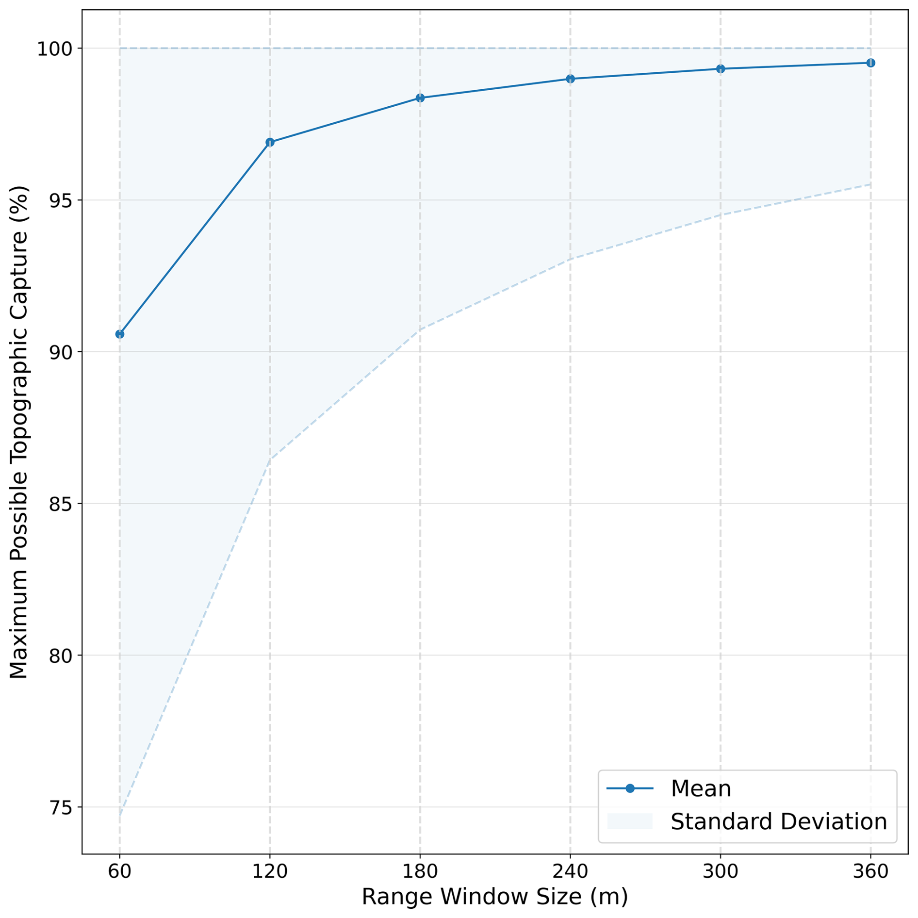
Figure 6 Maximum possible percentage of topography captured with optimal placement of the range window as a function of range window size. The shading shows the variability across records in the percentage of topographic capture, characterised by the standard deviations and limited at its maximum to 100 %.

6.3 Capture of the Point of Closest Approach

6.3.1 Level-2-Derived Point of Closest Approach (LPC)

Next, we analysed the positioning of the POCA identified in the Level-2 product, relative to the range window and beam-limited footprint, and compared this to the positioning of the geometric point of closest approach, as determined by minimising the distance between the satellite and the REMA surface. In practice, this was done by classifying every measurement according to its positioning relative to the range window (Fig. 7a). In order to explore how performance varied spatially, we binned the L2 POCA classes (LPCs), and the REMA-derived POCA classes (RPCs) to 5 km (Figs. 7b and 8b). As these data are discrete, the modal values were taken, so as to provide the most common class within each grid cell. Using our new slope and roughness derivations (Fig. 2), we also explored the relationships between these window placement classes and the topographic parameters (Figs. 7 and 8).

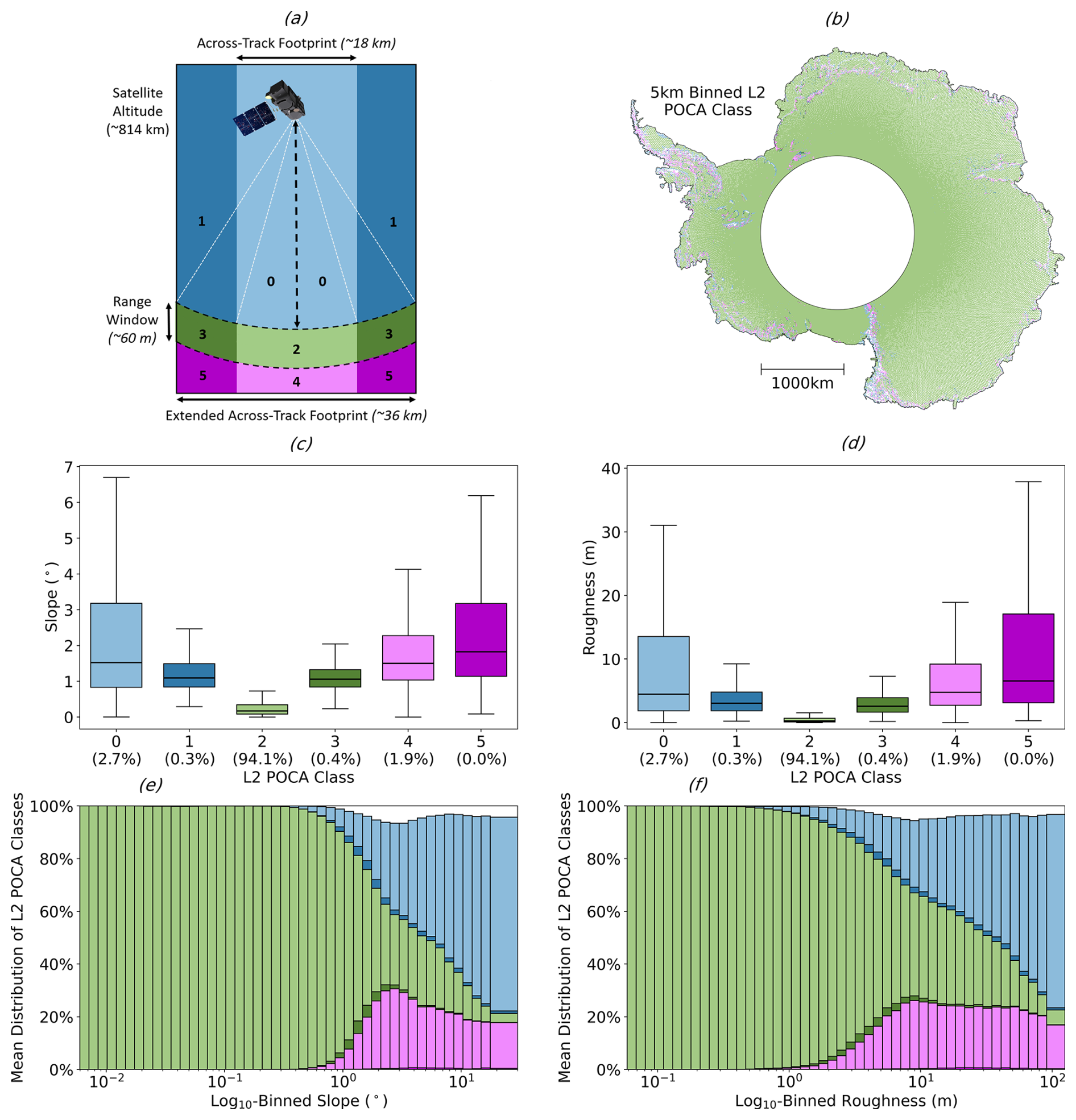
Figure 7 Assessment of the ability of Sentinel-3 to capture the surface reflection at the L2-derived POCA. Panel (a) outlines the POCA class definitions as per Fig. 1 for ease of cross-referencing. Panel (b) shows the L2-derived POCA classes, spatially binned to 5 km. Panels (c) and (d) show box plots of the L2-derived POCA per-class distribution with respect to slope and roughness, with the percentage of data within each class given in parentheses. Panels (e) and (f) show stacked bar charts representing the percentage distribution of the L2-derived POCA classes within each slope and roughness bin.

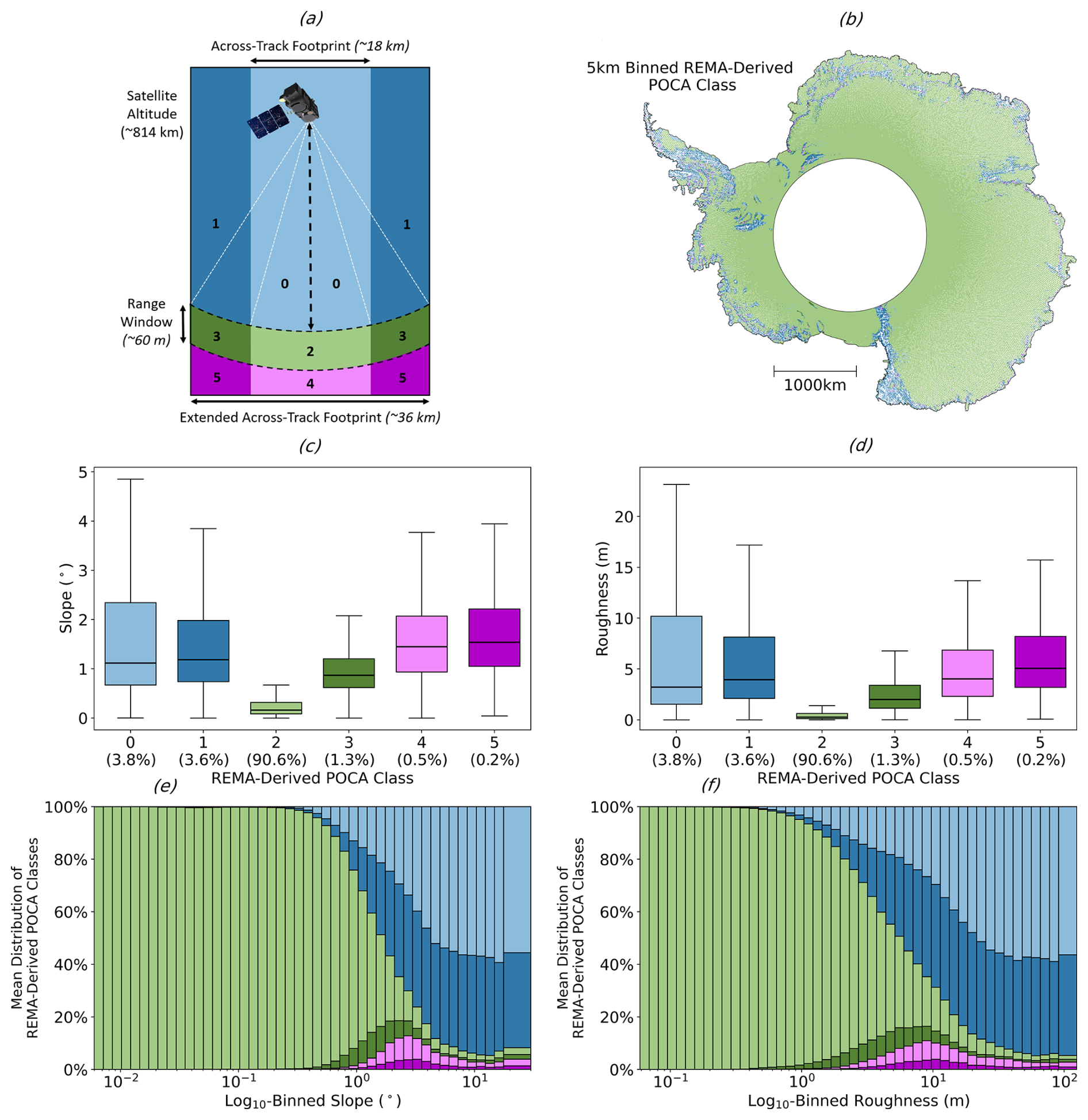
Figure 8 Assessment of the ability of Sentinel-3 to capture the surface reflection at the REMA-derived POCA. Panel (a) outlines the POCA class definitions as per Fig. 1 for ease of cross-referencing. Panel (b) shows the REMA-derived POCA classes, spatially binned to 5 km. Panels (c) and (d) show box plots of the REMA-derived POCA classes with respect to slope and roughness. Panels (e) and (f) show stacked bar charts representing the percentage distribution of the REMA-derived POCA classes with respect to log₁₀-binned slope and roughness.

As a result of quality control and filtering in the L2 processing, we observe that ∼ 0.447 % of the data is missing for the LPCs within the BC-005 product. This represents a significant improvement compared to the previous BC-004 product, wherein ∼ 3.20 % of the data were missing, primarily over topographically complex areas. The proportion of missing data increases with slope and roughness, comprising 5 %–10 % of samples in regions of very high slope and roughness (Fig. 7e and f, respectively). For 94.1 % of the full, non-aggregated data, we observe that the L2 POCA lies within both the Sentinel-3 beam-limited footprint and the range window. This occurs almost exclusively in regions of lower slope and roughness, with a median of 0.170° and 0.277 m, and median absolute deviation of 0.105° and 0.189 m respectively (Fig. 7c and d). In contrast, the remaining 5.9 % of acquisitions where the L2 POCA fails to be located within the range window encompass a far greater range of slope and roughness values, retaining significantly higher medians. This is evident spatially, with LPCs with a value other than 2 grouped around areas of complex topography such as the Transantarctic mountains, the Antarctic Peninsula, and coastal regions (Fig. 7b). Comparing to the performance of the BC-004 product, again we find that the evolutions in BC-005 offer an improved capacity to derive a POCA that is consistent with the range window. Specifically, we find that BC-004 returned a lower (89.5 %) percentage of records where the L2 POCA was correctly located within the range window and beam footprint (i.e. LPC class 2). Thus, the switch from BC-004 to BC-005 has approximately halved the proportion of acquisitions where the prescribed POCA location and the range window position are inconsistent.

We find that the proportion of L2 POCA's falling within both the beam-limited footprint and the range window (class 2) decreases with increasing slope and roughness. For both covariates (Fig. 7e and f), the relationship follows trends similar to those reported for topographic capture in Sect. 6.2.1. We find that for surface slopes (roughness) up to ∼ 0.3° (∼ 0.3 m), the current window placement achieves near to 100 % capture of the POCA location. As slope increases beyond this limit, however, the proportion of class 2 decreases, such that by ∼ 1° only ∼ 70 % of the L2 POCA's lie within the desired range, and by ∼ 5° this reduces further to ∼ 30 % (Fig. 7e and f). Likewise for roughness, we observe a reduction in the proportion of class 2 with increasing roughness, wherein by ∼ 10 m the proportion of LPCs of class 2 reduces to ∼ 40 %, and further to ∼ 20 % by ∼ 50 m (Fig. 7e and f). With increasing slope and roughness, the observed reductions in class 2 are replaced in approximately equal parts by classes 0 (POCA above the range window ) and 4 (POCA below the range window), up until ∼ 3° slope and ∼ 1 m roughness, wherein the increase in proportion of class 4 plateaus, and classes 0 dominate towards the extremes. This likely reflects the inability of the linear slope correction to adequately identify a point within the range window, in regions of high topographic variability. Notably, the occurrences of classes 1, 3, and 5, which constitute POCA locations outside of the beam-limited footprint, are negligible (0.3 %, 0.4 %, and 0.0 %, respectively), and much lower than found in BC-004 (1.1 %, 0.7 %, and 0.7 % respectively), likely a result of the algorithmic decision to avoid relocations beyond the 3 dB beamwidth.

6.3.2 REMA-Derived Point of Closest Approach (RPC)

The RPCs, which are defined using the location that minimises the range between the surface and satellite, rather than the location written in the L2 product, follow broadly the same distribution as the LPCs, with the exception of minimal data loss (∼ 0.00261 %), which is simply due to missing data within the REMA dataset (Fig. 8b). Overall, 90.6 % of the full, non-aggregated data has an RPC of 2 (corresponding to a POCA within both the beam-limited footprint and range window), with median slope and roughness for this class of 0.163° and 0.259 m, respectively (Fig. 8c and d). Notably, the BC-004 product classifies a slightly reduced 89.0 % of class 2 RPCs, indicating improvements in the BC-005 product in its ability to capture the “true” POCA (as defined by REMA), due to the extended window processing. The level of agreement on an RPC classification of 2 between the two product versions varies significantly with surface slope. For slopes of 0.0–1.0, 1.0–2.5, and ≥ 2.5°, the percentage of records for which BC-004 and BC-005 agree is 93.6 %, 19.0 %, and 3.25 %, respectively, illustrating the impact that the refined BC-005 processing is having for retrievals in topographically complex areas. In these same slope bins, the percentage of acquisitions where BC-005 correctly returns a class 2 classification, whereas BC-004 does not, is 1.93 %, 13.8 %, and 1.88 %; whereas the converse case where BC-004 returns class 2 and BC-005 does not, occurs for only 0.766 %, 3.04 %, and 0.832 % of records. A similar pattern is observed with respect to surface roughness. For roughness ranges of 0.0–5.0, 5.0–10, and ≥ 10 m, the percentage of records where BC-005 returns class 2 and BC-004 does not is 2.45 %, 8.26 %, and 2.10 %, whereas the converse occurs for only 0.845 %, 2.59 %, and 1.23 % of acquisitions. Together, these observations illustrate the improvements delivered by the latest baseline, and suggests that the extended window processing implemented in BC-005 is able to more reliably track the POCA in regions with more complex topographic terrain. Nonetheless, the fact that 64.1 % and 94.0 % of acquisitions in regions of 1.0–2.5 and ≥ 2.5° slope, respectively, do not have a REMA-derived POCA within the range window for either BC-004 or BC-005 illustrates the challenges presented by the relatively small 60 m range window in areas of complex topography, and the opportunity for further algorithmic evolution.

In comparison to the LPC's, the RPCs return more cases where the POCA is located above the range window, and less instances where the POCA is below the range window (Fig. 8c and d). This is unsurprising given that the RPC approach, by minimising the range, favours the highest point within the footprint, which is more often above rather than below the range window. With respect to slope and roughness, the RPCs exhibit similar trends in class 2 as the LPCs, although there is a greater proportion of measurements located outside of the 3 dB beamwidth (classes 1, 3, and 5), corresponding to the half-power limit of the antenna gain pattern (±9.1 km across-track) where signals are significantly attenuated. The higher proportion of RPCs in these outer classes reflects that our REMA-based approach uses an extended 36 km across-track search diameter and does not impose restrictions on POCA location, whereas the L2 processing algorithm limits relocations to within the beamwidth. Whilst the 3 dB threshold provides a physically meaningful and historically grounded boundary for the antenna illumination area, this analysis demonstrates that in topographically complex terrain, the geometric point of closest approach can lie beyond this limit.

The proportion of classes 0 and 1 increases with slope and roughness in approximately equal parts, however, unlike the LPCs, classes 4 and 5 experience only a temporary increase with increasing slope and roughness, peaking at ∼ 3° and ∼ 9 m, respectively, before being replaced by classes 0 and 1 for more extreme topographic variance (Fig. 8e and f). We also find that classes 4 and 5 often occur at the transition between floating and grounded ice (Fig. 8b), where there is a rapid change in the surface gradient, and hence may be due to the inertia in the closed-loop tracker, which positions the range window based upon preceding tracker information. As slope and roughness increase further, then classes 0 and 1 again dominate, reflecting the behaviour typical of mountainous terrain where local topographic highs exceed the positioning of the range window.

6.3.3 Impact of Satellite Heading at the Ice-Ocean Transition

Lastly, we again assessed whether the per-class distribution was affected by the satellite heading for acquisitions made within close proximity (within 30 km) of the ice sheet coast. For the RPCs, we observed that the range window was adequately placed (i.e. class 2) for 50.4 % of the measurements that were acquired when heading from land to ocean, and 51.6 % when heading from ocean to land. A difference of only ∼ 1.2 % suggests that there is no definitive evidence that coastal heading affects the per-class distribution close to the ice sheet coast, similar to the negligible difference in topographic capture rate (with respect to the theoretical maximum) that was observed in Sect. 6.2.3.

6.4 Along-track Correlation of Echoes

Our final set of analyses focuses on exploiting our new slope and roughness datasets to assess the correlation of series of altimetry echoes acquired along the orbit track, with a view to investigating the impact of surface topography on the degree of waveform correlation achieved. To investigate correlation across the entire ice sheet, we bin both the correlation between consecutive waveforms, and the fitted 50-record correlation change, taking the mean values within each 5×5 km grid cell (Fig. 9a and b). For the inter-record correlation, we found a median of 0.944 and a median absolute deviation of 0.003, with the distribution skewed towards higher correlation values, and lower values grouped around areas of topographic complexity (Fig. 9a). For the fitted 50-record correlation change, we found a median reduction in the correlation of −0.418 over 15 km and a median absolute deviation of 0.025. 12.6 % of records had a correlation change of less than −1 and were removed from our analysis (as discussed in Sect. 5.4). By comparing qualitatively to our REMA-derived estimates of across-track surface slope and roughness (Fig. 2), it is clear that both of these topographic parameters influence the degree of correlation between waveforms. For example, correlation reduces in areas of high roughness, such as megadune fields in East Antarctica, and high surface slope, such as the coastal margin of the ice sheet (Fig. 9a and b).

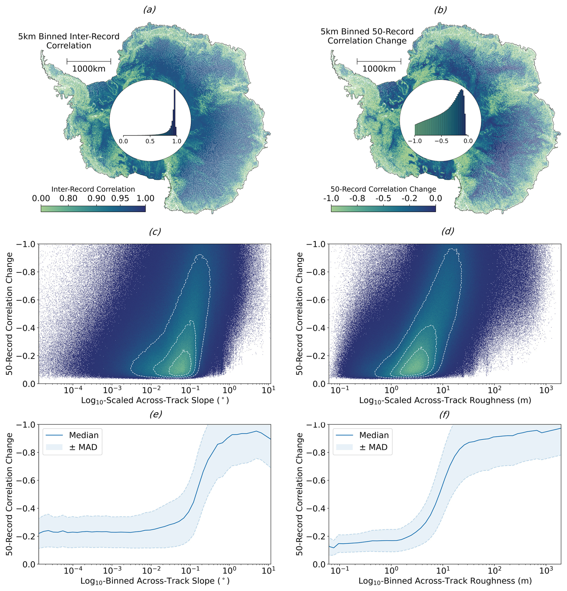
Figure 9 Analysis of the along-track correlation of Sentinel-3 SAR altimetry echoes. Panel (a) shows the correlation between consecutive records, spatially binned to 5 km. Panel (b) shows the 50-record correlation change, also spatially binned to 5 km. Histograms showing the overall distribution of each parameter are given within the pole holes of the respective plots. Panels (c) and (d) show density plots of the 50-record correlation change as a function of log₁₀-binned slope and roughness respectively. Concentric contours are included, which contain 75 %, 50 %, and 25 % of the data from outside to in respectively. Panels (e) and (f) show the median and median absolute deviation of the 50-record correlation change with respect to log₁₀-binned slope and roughness, respectively.

Comparing the fitted 50-record correlation change to across-track surface slope and roughness, we see that the 15 km change in correlation remains relatively stable at ∼ −0.25, for slopes up to ∼ 0.01°, before dropping rapidly to ∼ -0.95 for slopes above this value (Fig. 9e). For low surface roughness, the 50-record correlation change is ∼ −0.15, but this quickly drops towards ∼ −1 once roughness exceeds ∼ 2 m (Fig. 9f). Taking the Pearson correlation coefficient of the 50-record correlation change to log₁₀-binned surface slope and roughness we find values of −0.618 and −0.571. This implies that, linearly, slope and roughness explain 38.2 % and 22.2 % of the ice-sheet wide variance in along-track waveform decorrelation. We therefore conclude that 50-record correlation change is moderately, linearly correlated to log₁₀-binned surface slope and log₁₀-binned roughness, with slope providing a stronger control. Whilst conceptually, it is understood that slope and roughness impact the shape of the echo, and associated parameters such as the number of peaks, leading edge width, and trailing edge slope, this analysis demonstrates quantitatively the strength of this correlation, through the comparison of independent altimetry and DEM-derived datasets.

7 Conclusions

Since the launch of Sentinel-3A in 2016, and Sentinel-3B in 2018, the Sentinel-3 mission has acquired hundreds of millions of echoes over Antarctica, providing topographic information at a resolution of ∼ 300 m along-track by ∼ 1.6-2 km across-track, which are repeated every ∼ 27 d. To date, however, previous assessments of Sentinel-3 performance over ice sheets have concentrated predominantly on the outputs of L2 processors, namely the high-level validation of the resulting elevation products. Here, we extend previous work by using novel topographic datasets derived from REMA, to more directly explore the underlying factors that influence Sentinel-3's performance. Specifically, we use Singular Value Decomposition to robustly separate local elevation variability into slope and roughness components, and investigate the impact of each upon Sentinel-3 altimeter performance.

Quantitatively, our new estimates of slope and roughness indicate a strong positive correlation between these two variables; areas with higher surface slopes also exhibit greater kilometre-scale (orthogonal) surface roughness. Overall, we find that 76.9 % and 89.1 % of the ice sheet exhibits slopes below 0.5 and 1.0°, respectively; and 62.4 % and 76.1 % has a roughness lower than 0.5 and 1.0 m,respectively (where roughness is defined as the minimum- to-maximum difference of the orthogonal residuals). Our SVD-based approach explicitly decouples these parameters, yielding – to the best of our knowledge – the first continent-wide analysis of Antarctic surface roughness that is independent of slope.

During operation, the Sentinel-3 onboard tracker aims to position the range window so that it captures the underlying topographic surface. One way to measure its success in doing so, whilst acknowledging the inherent limitations imposed by the range window dimension, is to assess the proportion of the surface illuminated by the instrument that falls within the range window. Performing such an assessment at the ice sheet scale, through the analysis of over 8 million echoes, we find that in 57.4 % of cases, capturing the full topography within the beam-limited footprint is impossible, due to the relatively small ∼ 60 m range window of Sentinel-3, relative to the high topographic variance found across some regions of the ice sheet. Nonetheless, our analysis shows that with optimal placement of the range window, 80 % of the illuminated topographic surface could be captured in ∼ 80 % of cases. Building on this, we investigated the performance of the current window placement, by measuring the ratio of actual topographic capture to the maximum possible capture that could be achieved with an adjusted placement of the range window. On average, the current placement achieved a median of 89.2 ± 2.46 % of total possible topographic capture, with this value decreasing with increasing slope and roughness. Broader analysis of the relationship between range window size and maximum achievable topographic capture demonstrates that substantial gains are possible by increasing the window beyond 60 m. Doubling the window to 120 m, for example, increases the mean capture from 90.6 % to 96.9 % and reduces variability (standard deviations of 15.9 % and 10.5 %, respectively). This indicates that a 60 m window is a limiting threshold in complex terrain, where vertical relief within the illuminated footprint frequently exceeds the available range. Adopting wider windows – such as the 256 m range window planned for the CRISTAL mission – substantially reduces this limitation. Overall, this analysis provides empirical support for future mission design, by quantifying the range window dimensions required to enable near-complete topographic capture of the ice sheet margins.

Within current L2 processing schemes, there is an implicit assumption that the prescribed point of closest approach (POCA) lies within both the instrument's beam-limited footprint and its range window, and hence that the range to the waveform leading edge corresponds to the distance between the satellite and the identified POCA. To evaluate this assumption, we compared the locations of the L2-designated POCA in two product versions (BC-004 and BC-005) to the position of range window for ∼ 8 million acquisitions collected over the Antarctic Ice Sheet, in addition to that of an independent POCA estimate that we derived from a high resolution DEM. This analysis showed that the current window placement successfully captures the point of closest approach for 90.6 % of acquisitions and allowed us to investigate, quantitatively, the improvements offered by the BC-005 extended window processing, in areas of complex topographic terrain.

Finally, we explored the correlation between sequences of altimetry echoes along the satellite orbit track, to provide a first assessment of how surface topography affects waveform decorrelation. We found that inter-record correlation was generally high, but decreased in areas with complex topography. Similarly, the larger-scale correlation change across 50-records (spanning ∼ 15 km) indicated that the rate of decorrelation was more rapid in regions with high surface slope and roughness. While the relationship between topography and waveform decorrelation is conceptually well established, this analysis provides new quantitative evidence of these effects at the ice sheet scale, with slope and roughness explaining 38.2 % and 22.2 % of the variance in along-track decorrelation, respectively. These metrics offer empirical support for understanding how surface morphology influences waveform structure.

More broadly, this study has shown how a new generation of high-resolution DEMs can be used to assess and understand the performance of current altimetry in-flight systems and on-the-ground processing. This information provides new insight to help understand the current performance of the Sentinel-3 fleet of satellite altimeters, and also serves as a template for future analysis that can guide the design and optimisation of planned missions such as the Copernicus Polar Ice and Snow Topography Altimeter (CRISTAL) and the Sentinel-3 Next Generation Topography mission.