Active-source seismic characterization of subglacial lakes: numerical modeling, field validation, and implications for Antarctic exploration

Subglacial lakes offer unique opportunities to study ice sheet dynamics, microbial life, and climate evolution. Motivated by the upcoming seismic survey of Qilin Subglacial Lake, this study constructs a representative subglacial lake model and extends it to six geological scenarios to examine their effects on seismic wavefield characteristics, revealing the prominent occurrence of guided waves and multiple reflections. Simulated data are then analyzed to identify key imaging challenges – particularly those arising from strong multiples, low-velocity firn layers, and source-side ghosts – and to assess processing strategies, such as salt flooding, that enhance imaging accuracy and suppress noise. Commonly used seismic acquisition systems in polar regions are also reviewed to summarize their characteristics and implications for survey design. Finally, four seismic lines from Lago Subglacial CECs are processed, demonstrating strong consistency with the simulation results in terms of key seismic features, thereby validating the proposed theoretical approach. Collectively, these efforts provide a robust and broadly applicable framework for understanding seismic wave propagation in subglacial lake environments, offering both theoretical insights and methodological guidance for future Antarctic investigations.

1 Introduction

Antarctica hosts over 760 subglacial lakes beneath ice layers several kilometers thick (Wilson et al., 2025), existing under extreme conditions of high pressure, freezing temperatures, darkness, and nutrient scarcity (Siegert, 2018; Livingstone et al., 2022). These lakes provide unique windows into early Earth environments and potentially analogous conditions on other planetary bodies. Their microbial communities and associated biogeochemical cycles offer insights into life evolution on Earth (Christner et al., 2014; Mikucki et al., 2016) and the search for extraterrestrial life (Garcia-Lopez and Cid, 2017). The sedimentary deposits at their bases record geological and climatic changes preceding ice sheet formation, making these lakes invaluable archives for understanding Antarctic ice sheet evolution and global climate change (Filina et al., 2007; Bentley et al., 2011; Smith et al., 2018; Yan et al., 2022; Siegfried et al., 2023). Hydrologically active lakes (Siegfried and Fricker, 2018), interconnected via subglacial channels (Wingham et al., 2006), can modulate basal ice shear stress, influencing ice flow, stability, and mass balance (Stearns et al., 2008; Horgan et al., 2012; Li et al., 2021), while delivering freshwater and nutrients to the Southern Ocean (Livingstone et al., 2013; Pattyn et al., 2016; Vick-Majors et al., 2020).

The West Antarctic Ice Sheet (WAIS), resting on the seafloor, is particularly sensitive to climate change due to its intrinsic instability (Joughin and Alley, 2011). Modeling suggests that during deglaciation tens of thousands of years ago, ice above the Whillans and Mercer subglacial lakes fully melted and was replaced by seawater (Venturelli et al., 2023). These lakes experience drainage and recharge cycles spanning months to years (Winberry et al., 2009; Siegert et al., 2016), with water flowing between lakes through subglacial channels before discharging into the ocean (Napoleoni et al., 2020). In contrast, the East Antarctic Ice Sheet (EAIS) rests largely on bedrock above sea level (Cui et al., 2020b; Glaciers, 2024), having formed approximately 34 million years ago and reached its present extent around 14 million years ago (Contributors, 2024). As a result, East Antarctic subglacial lakes have remained isolated and stable over geological timescales, preserving critical records of Earth’s climate and ice sheet evolution (Jamieson et al., 2023).

Over the past decades, active-source seismic surveys have been applied to a limited number of Antarctic subglacial lakes, providing high-resolution profiles of ice thickness, lake boundaries, and basal sediments. The earliest seismic investigation associated with a subglacial lake was conducted near Vostok Station in 1959, when Andrey P. Kapitsa and colleagues performed reflection soundings to determine ice thickness. Although the strong basal reflections they recorded were not recognized as subglacial water at the time, later analyses combining these seismic data with satellite altimetry confirmed the existence of Lake Vostok beneath approximately 4 km of ice (Ridley et al., 1993; Kapitsa et al., 1996). In 2008, Peters et al. conducted an active-source seismic reflection survey over Lake 63 (South Pole Lake) to investigate a radar-identified subglacial lake near the geographic South Pole. The survey revealed an ice thickness of about 2857 ± 15 m and confirmed the presence of liquid water through AVO analysis, with a lake water column of 32 ± 10 m, as well as underlying thick sedimentary strata (Peters et al., 2008). Between the 2007/08 and 2008/09 field seasons, the British Antarctic Survey (BAS) conducted active-source seismic surveys over subglacial Lake Ellsworth in West Antarctica. Five seismic lines (labeled A–E) were acquired, imaging ice thickness varying from roughly 2450 m to 2550 m, with lake water depths ranging between approximately 50 and 120 m (Woodward et al., 2010). During the 2010/11 Antarctic field season, the WISSARD project conducted active-source seismic surveys over Whillans Subglacial Lake (SLW) in West Antarctica. Four seismic lines were acquired, imaging a lake water column of 2–10 m beneath an ice sheet approximately 800 m thick (Horgan et al., 2012). Active-source seismic surveys over subglacial Lake CECs in West Antarctica were jointly conducted by the British Antarctic Survey (BAS) and the Centro de Estudios Científicos (CECs). In 2016, four seismic lines were acquired, followed by an additional line in 2022, imaging an ice thickness of approximately 2650 m and a lake water column of 301 m. Seismic imaging and reflection analysis suggest a soft sediment layer in the central section pf the lake bed, with a thickness of approximately 15 m (Brisbourne et al., 2023b). Active-source seismic surveys over Subglacial Lake D2 (SLD2) beneath David Glacier in East Antarctica were conducted by the Korea Polar Research Institute (KOPRI). In the 2021/22 austral summer, four seismic lines were acquired, imaging an ice thickness ranging from approximately 2250 to 2300 m and a lake water column varying between 53 and 82 m (Ju et al., 2026). Overall, these seismic investigations highlight the potential of active-source methods to resolve ice, water, and sediment structures in Antarctic subglacial lakes, providing a foundation for future high-resolution studies.

China has conducted extensive airborne geophysical surveys in Princess Elizabeth Land using the Snow Eagle 601 aircraft (Cui et al., 2018, 2020a), leading to the discovery of Lake Qilin, a large and hydrologically stable subglacial lake buried over 3000 m beneath the ice (Yan et al., 2022). However, existing airborne surveys cannot provide precise information on the internal structure of the lake and its underlying sediment layers, highlighting the need for high-resolution seismic exploration to resolve these features. Motivated by the upcoming seismic exploration of Lake Qilin, this study aims to advance understanding of seismic responses in subglacial lake environments and provide broadly applicable insights for future Antarctic investigations. A representative velocity model is constructed, and a systematic analysis of wavefield simulation, seismic data processing, and seismic acquisition system evaluation is carried out. Wavefield simulations are first performed to examine how key polar geological structures – such as subglacial lakes, firn layers, sediments, and the free surface – influence seismic wavefield characteristics. Synthetic seismic data derived from these models are then analyzed to identify challenges in conventional seismic processing – particularly those related to firn-layer effects and multiple reflections – and to explore potential strategies, including salt flooding, for improving subglacial lake imaging. In addition, three commonly used seismic acquisition systems in polar regions are evaluated to characterize their properties and potential suitability for subglacial lake studies, offering guidance for planning field acquisition strategies. Finally, four seismic lines from Lago Subglacial CECs are processed and analyzed, with results that both corroborate the key findings from the simulations and data processing experiments and provide insights into the lake’s internal structure. Overall, this work offers a reference framework for investigating seismic responses in subglacial lakes and supports planning of future Antarctic field campaigns.

2 Seismic Wavefield modeling of Subglacial Model

Figure 1a illustrates a typical subglacial velocity model, with a depth of 3.6 km and a horizontal extent of 10 km. The model consists of a thick ice sheet, a subglacial lake, and the underlying bedrock.

• The ice sheet thickness is set to 2400 m, representing the average value of the ice cover above the subglacial lake as documented in Table 1, and the P-wave velocity of the ice is set to 3800 m s⁻¹ (Yan et al., 2020).

• The lake-water P-wave velocity is set to 1500 m s⁻¹, with a depth of 500 m (the shallowest reported for Lake Vostok), to ensure clearer wavefield separation within the water column while maintaining computational efficiency.

• In a similar manner, the sediment layer, used in a later section, is assigned a thickness of 200 m and a P-wave velocity of 2820 m s⁻¹, representing normal sediment(Horgan et al., 2012).

• Following an empirical firn model (Herron and Langway, 1980), a firn layer (applied in a later section) is prescribed with a thickness of 150 m, as firn in the Antarctic interior has been reported to exceed 100 m in thickness.

• The bedrock beneath the lake has a P-wave velocity set to 5200 m s⁻¹ (Peters et al., 2008).

• To emphasize the influence of contrasting material properties (e.g., lake water, sediments, firn) on the simulated wavefield, a simplified lake geometry is employed, characterized by a flat central bed and sloping lateral margins.

Table 1 Summary of Documented Subglacial Lake Parameters (Peters et al., 2008; Woodward et al., 2010; Siegert et al., 2011; Horgan et al., 2012; Priscu et al., 2021; Brisbourne et al., 2023b; Ju et al., 2026).

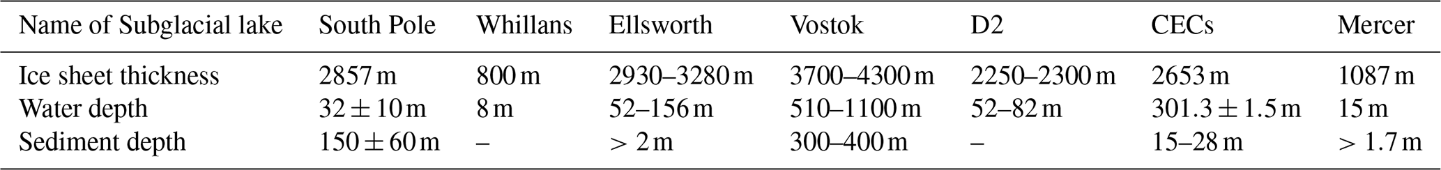
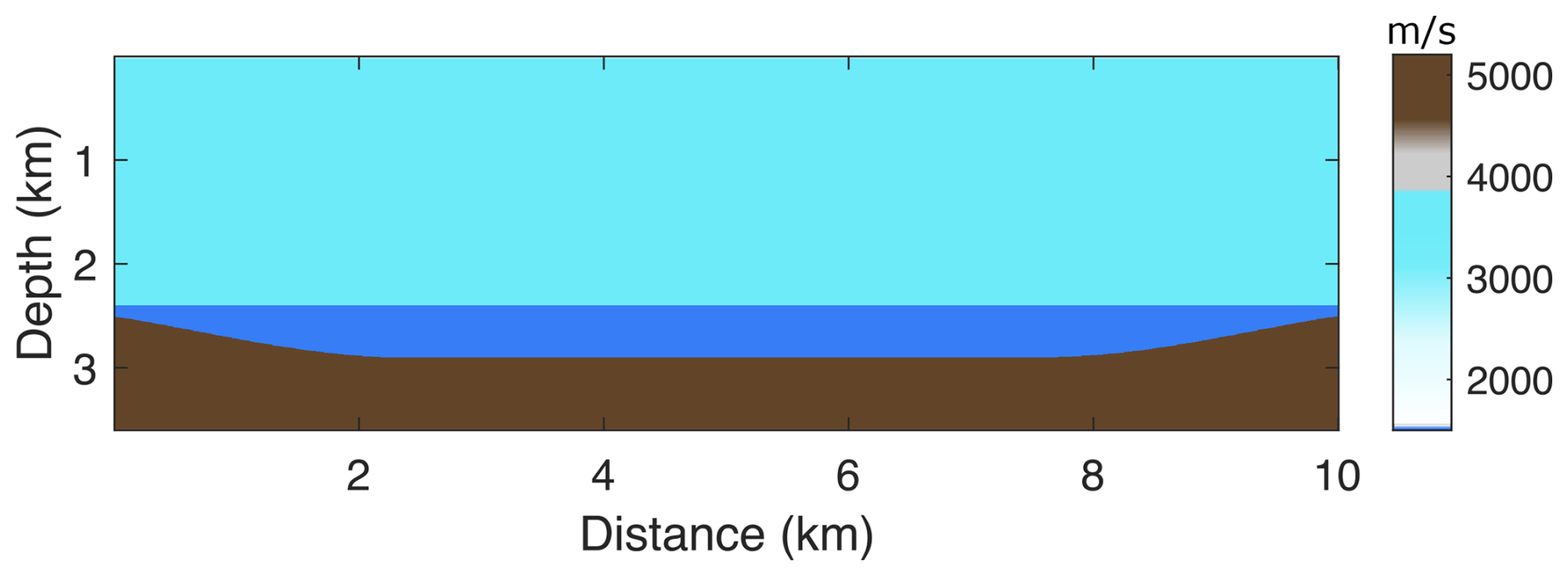
Figure 1 A typical subglacial velocity model with an ice sheet, a subglacial lake and bedrock.

Building upon this model, we systematically investigate the seismic wavefield propagation characteristics under various conditions, including absorbing boundaries, firn layers, the free surface, and sediment layers, as well as their combinations. The wavefield simulation is performed using a first-order acoustic wave equation within a staggered-grid finite-difference framework (Chen et al., 2020). Both the source and receivers are placed on the surface of the ice sheet, with receivers evenly spaced at 5 m intervals across the entire surface. A Ricker wavelet with a central frequency of 20 Hz is employed as the source, with a time sampling interval of 0.5 ms and a total simulation time of 5 s.

2.1 Absorbing boundary

When the model is surrounded by absorbing boundaries, seismic waves do not reflect upon reaching the model's edges. Consequently, wave propagation is primarily influenced by the subglacial geological structure and its elastic properties (velocity and density). The substantial impedance contrast between the ice sheet, subglacial lake, and bedrock leads to strong reflections at the ice-water and water-bedrock interfaces.

Figure 2 presents wavefield snapshots at various time steps. Upon triggering the source, a direct wave (Fig. 2a) is generated and propagates downward as a spherical wave. Upon reaching the ice-water interface (Interface 1), part of the energy is reflected, forming the primary reflection wave R₁ (Fig. 2b). Due to the significant impedance contrast between ice and water, the reflection coefficient at the ice-water interface is negative, resulting in a polarity reversal of the reflected wave. Additionally, a portion of the direct wave's energy transmits downward into the lake. When this energy reaches the water-bedrock interface (Interface 2), it generates the primary reflection wave R₂ at the water-bedrock boundary (Fig. 2c and d). The reflected wave R₂ then propagates upward and partially reflects downward again at the ice-water interface, returning to the lake. This wave reflects once more at the ice-water boundary, forming a first-order interlayer multiple R₂R₁R₂ (Fig. 2e). This interlayer multiple continues to oscillate within the water layer, generating higher-order multiples.

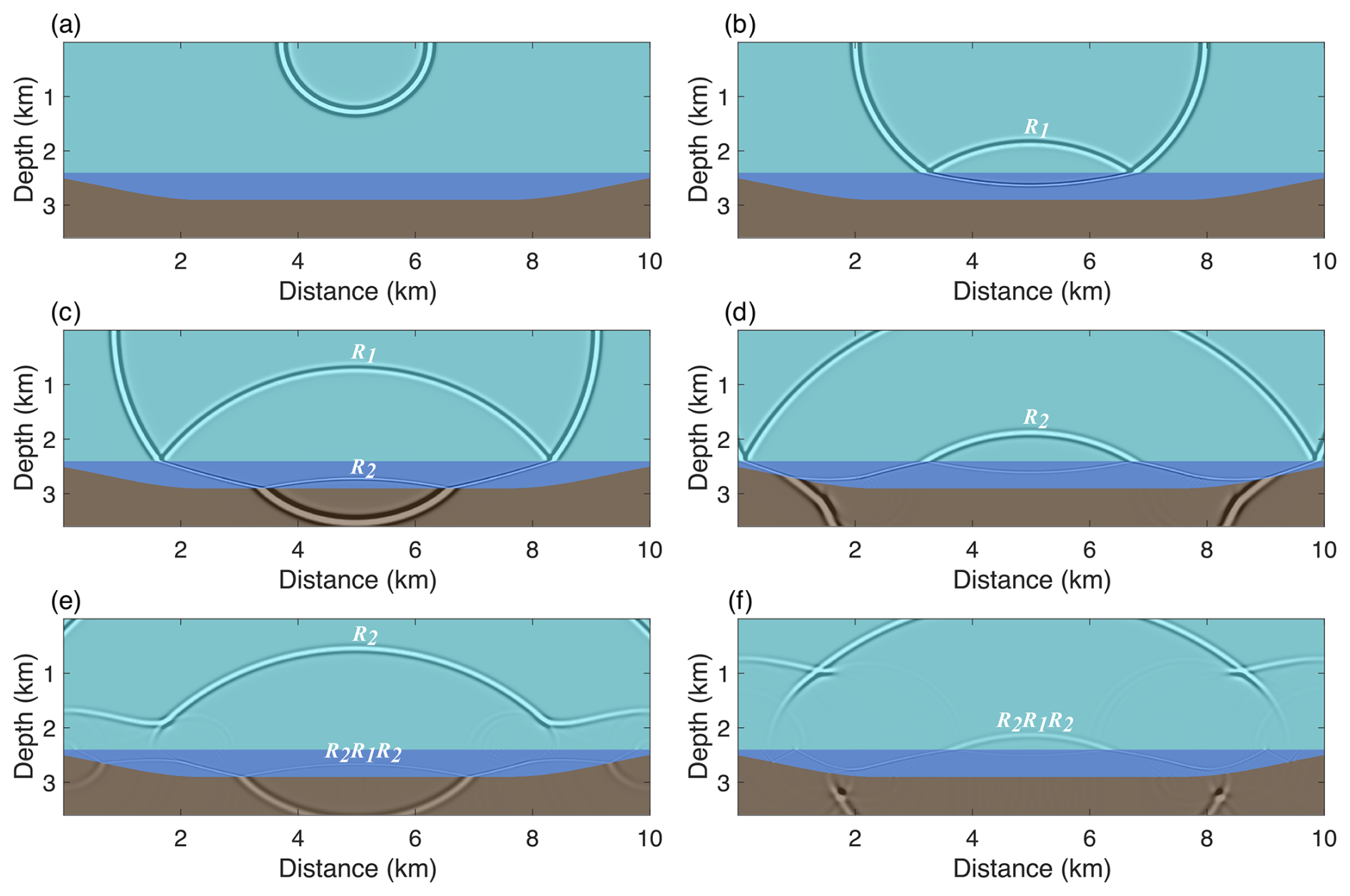
Figure 2 The wavefield snapshots at different time steps when the model is surrounded by absorbing boundaries, where (a) to (f) represent the wavefield snapshots at t=0.4, t=0.85, t=1.15, t=1.5, t=1.85, and t=2.1 s, respectively.

2.2 Free surface

The ice sheet surface represents a free surface, as the elastic properties of the overlying air are negligible compared with those of the ice, thereby satisfying the zero-stress boundary condition(Lan and Zhang, 2011). In this model, the ice sheet surface is treated as a free surface to investigate the effect of this boundary condition on seismic wave propagation.

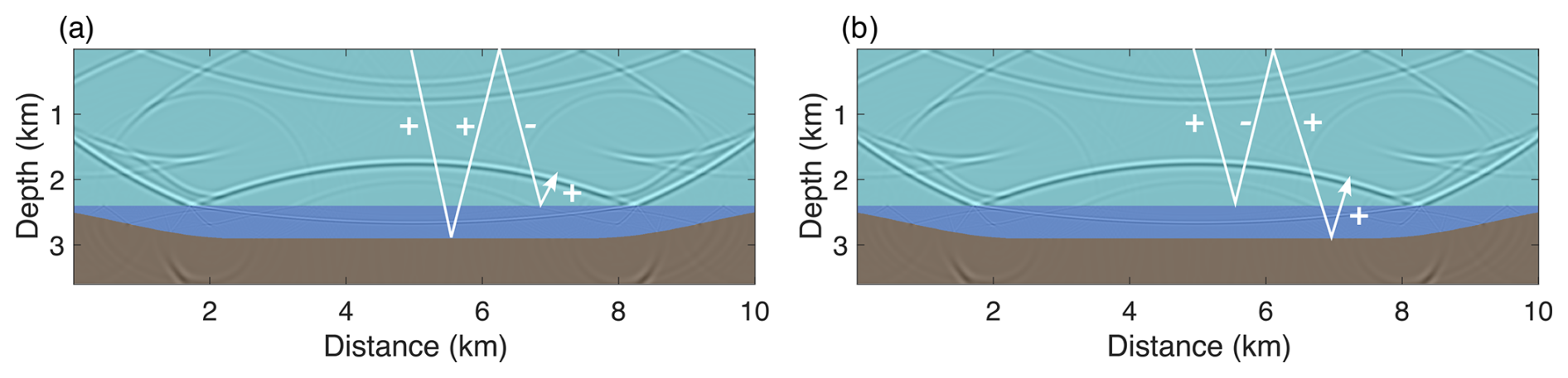
As illustrated in Fig. 3a, before reaching the surface, primary reflections R₁ and R₂ propagate similarly to the absorbing boundary case (Fig. 2c). Upon encountering the free surface, R₁ is fully reflected with reversed polarity (R₁F in Fig. 3b, c), as the surface acts as a boundary with reflection coefficient −1. The downward-propagating R₁F is partially reflected at the ice-water interface, generating first-order free surface multiples (R₁FR₁ in Fig. 3d), which continue to reflect between the surface and interface, producing second- and higher-order multiples (e.g., R₁FR₁FR₁ in Fig. 3f). Similarly, R₂ produces R₂FR₂ (Fig. 3e) and higher-order free surface multiples through the same mechanism. Reflections from the free surface can also propagate into the water layer, generating hybrid multiples (e.g., R₂FR₁ and R₁FR₂ in Fig. 3e and f). Their propagation involves complex interactions and repeated reflections among the ice, water, and free surface. Notably, R₂FR₁ and R₁FR₂ share the same propagation direction, velocity, arrival time, and polarity, leading to constructive interference and an amplified reflected wave. Ray path analyses of these multiples are shown in Fig. 4a and b.

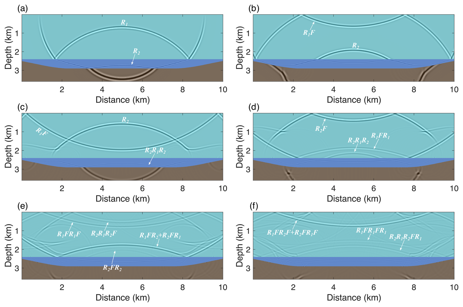
Figure 3 The wavefield snapshots at different time steps when the free surface is added to the top of the model, where (a) to (f) represent the wavefield snapshots at t=1.15, t=1.5, t=1.85, t=2.1, t=2.8, and t=3.45 s, respectively.

Figure 4 Demonstration of ray paths of free surface multiple (a) R₂FR₁ and (b) R₁FR₂.

2.3 Firn layer

Firn is a porous, transitional layer in polar ice sheets, located between freshly fallen snow and glacial ice (Hollmann et al., 2021). It covers about 99 % of the Antarctic ice sheet and roughly 90 % of the Greenland ice sheet, playing a vital role in understanding ice-sheet mass balance, hydrology, and paleoclimate (Diez et al., 2013; Schlegel et al., 2019; Humbert, 2024). The thickness of the firn layer ranges from a few meters to over 100 m across the ice sheets of Antarctica. Its density increases with depth due to the densification and metamorphosis of snow into glacial ice (Zhou et al., 2022; Pearce et al., 2022; Chaput et al., 2022). To assess the impact of the firn layer on wavefield propagation, we introduced a 150 m-thick firn layer, constructed using an empirical firn model (Herron and Langway, 1980), to the top of the ice sheet in our model (Fig. 5a). The velocity increases from 1333 to 3800 m s⁻¹, transitioning smoothly at the firn–ice interface (Fig. 5b), where the critical density is reached at approximately 22 m depth.

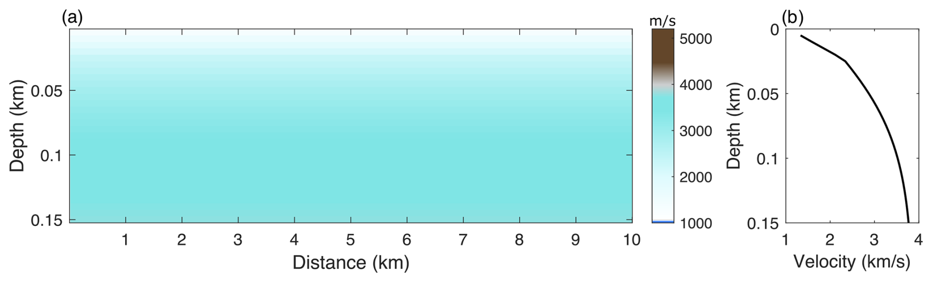
Figure 5 A zoomed-in view of the subglacial model showing the firn layer in the top 150 me, (b) the 1D vertical profile of the model shown in (a).

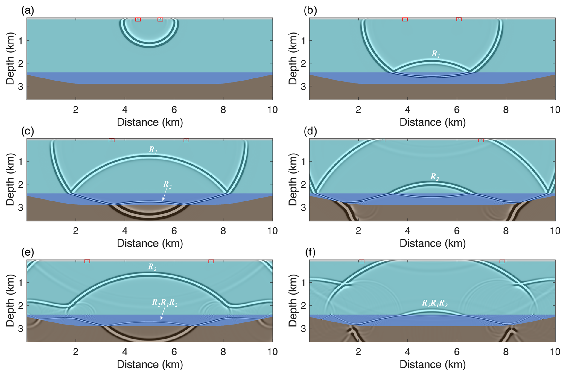
Figure 6 The wavefield snapshots at different time steps when a firn layer is incorporated into the subglacial model, where (a) to (f) represent the wavefield snapshots at t=0.4, t=0.85, t=1.15, t=1.5, t=1.85, and t=2.1 s, respectively.

Due to the significant velocity gradient within the firn layer, refracted waves emerge at relatively short offsets and propagate at the velocity of the underlying glacial ice. In contrast, the direct wave, within the red boxes in Fig. 6, travels more slowly along the surface at the velocity of the upper firn layer. This feature is more clearly illustrated in Fig. 7, which provides a zoomed-in view of the wavefield within the top 150 m. As a result, in seismic records, the first arrivals are primarily refracted waves, while the direct wave appears as a straight line with a steep slope (shown by the red dashed line in Fig. 12c).

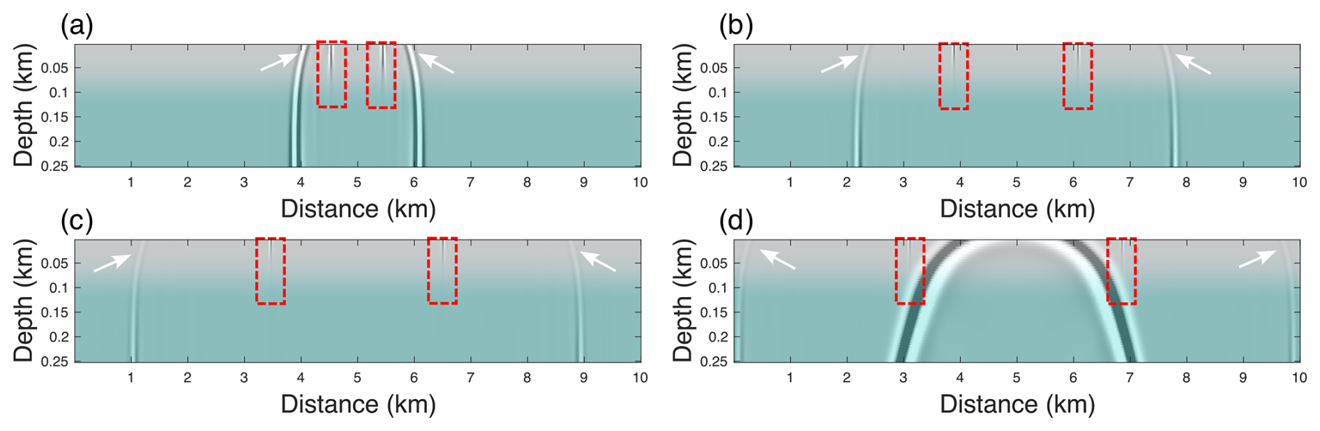
Figure 7 Zoomed in wavefield snapshots of the top 150 m at times t=0.4, t=0.85, t=1.15 and t=1.4 s.

2.4 Firn layer and free surface

In realistic settings, the firn layer coexists with the free surface and is included in our wavefield simulations. As shown in Fig. 8, a prominent feature is the generation of guided waves within the firn layer, which essentially correspond to multiple orders of the refracted wave. Their ray paths are shown in Fig. 9. Higher-order refracted waves appear at later times and require longer offsets for observation. In seismic records (Fig. 12d), these refracted waves are represented as a series of linear events with identical slopes, consistent time delays, and uniform offset intervals. Analyzing these guided waves provides valuable insights into the structure of the firn layer (Boiero et al., 2013; Li et al., 2018).

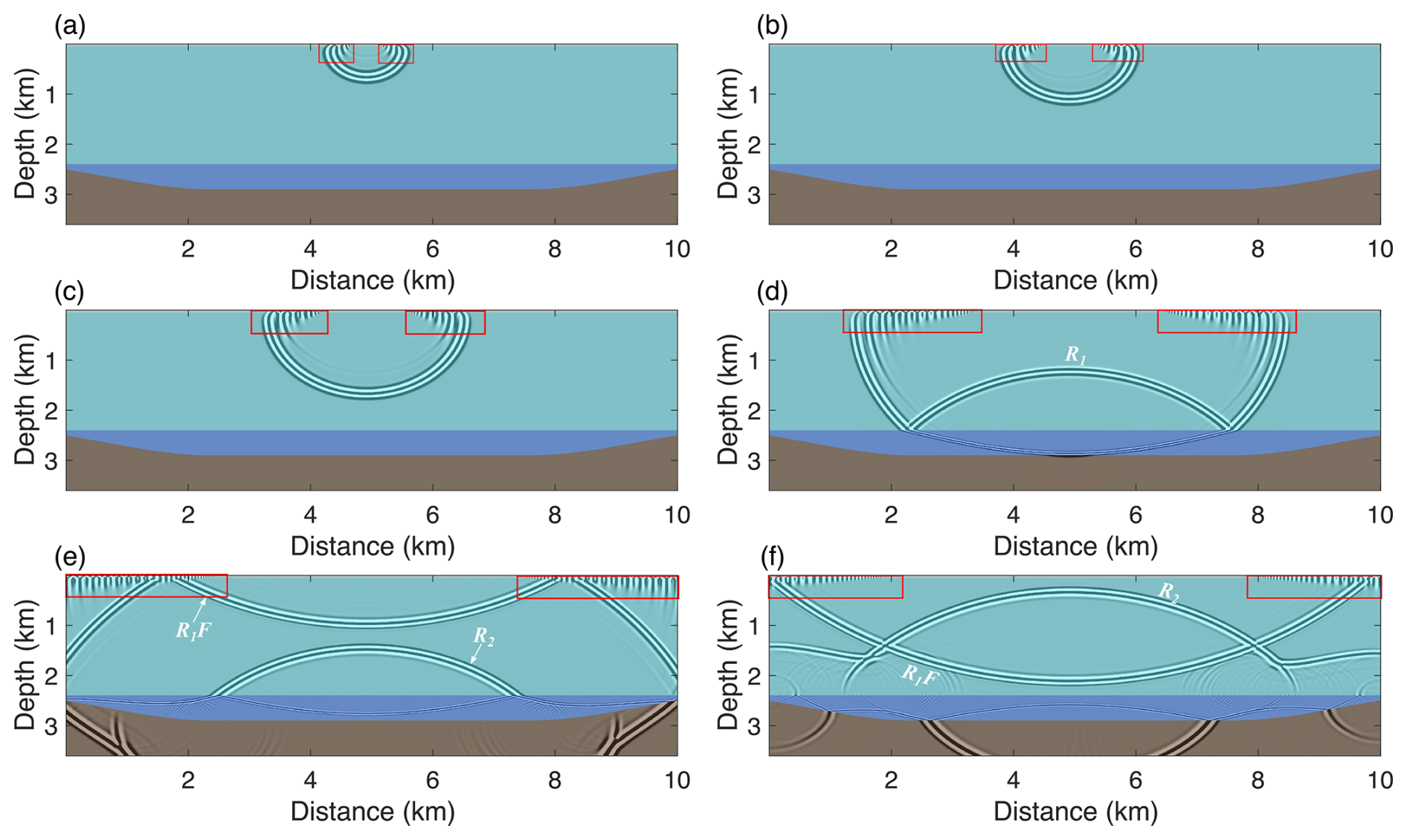
Figure 8 The wavefield snapshots at different time steps when both firn layer and free surface are incorporated into the subglacial model, where (a) to (f) represent the wavefield snapshots at t=0.2, t=0.35, t=0.5, t=1.0, t=1.6, and t=1.9 s, respectively.

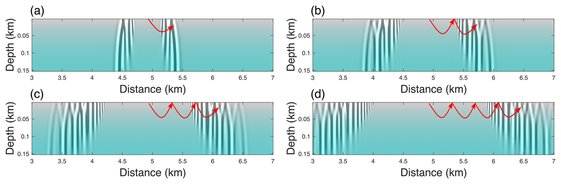
Figure 9 Zoomed in wavefield snapshots of the top 150 m at times t=0.2, t=0.35, t=0.5 and t=0.65 s.

2.5 Sediment layer

Sediment in subglacial lakes often contains paleoenvironmental records, such as those related to ice sheet history and climate change. These records are crucial for understanding past climate patterns, ice sheet dynamics, and geological history, all of which have significant scientific implications. To evaluate the impact of the sediment layer on seismic wave propagation, a 200m thick sediment layer with a velocity of 2820 m s⁻¹ (Peters et al., 2008; Maguire et al., 2021), was embedded within the lower part of the subglacial lake (Anandakrishnan and Winberry, 2004), while excluding the effects of the firn layer and free surface in our simulations.

The presence of a sediment layer introduces a significant feature: the generation of interlayer multiples within the sediment. As shown in Fig. 10b, the downgoing direct wave initially generates primary reflections R₁, R₂, and R₃ at the ice-water, water-sediment, and sediment-bedrock interfaces, respectively. Due to the thinness of the sediment layer, reflection R₃ quickly produces a first-order interlayer multiple, R₃R₂R₃, within the sediment shown in Fig. 10c. This interlayer multiple continues to oscillate within the sediment, generating higher-order multiples. Furthermore, reflections R₂ oscillate within the water layer, forming a first-order interlayer multiple, R₂R₁R₂, within the water layer (Fig. 10d), and R₂R₁R₃ across both the sediment and water layers (Fig. 10e).

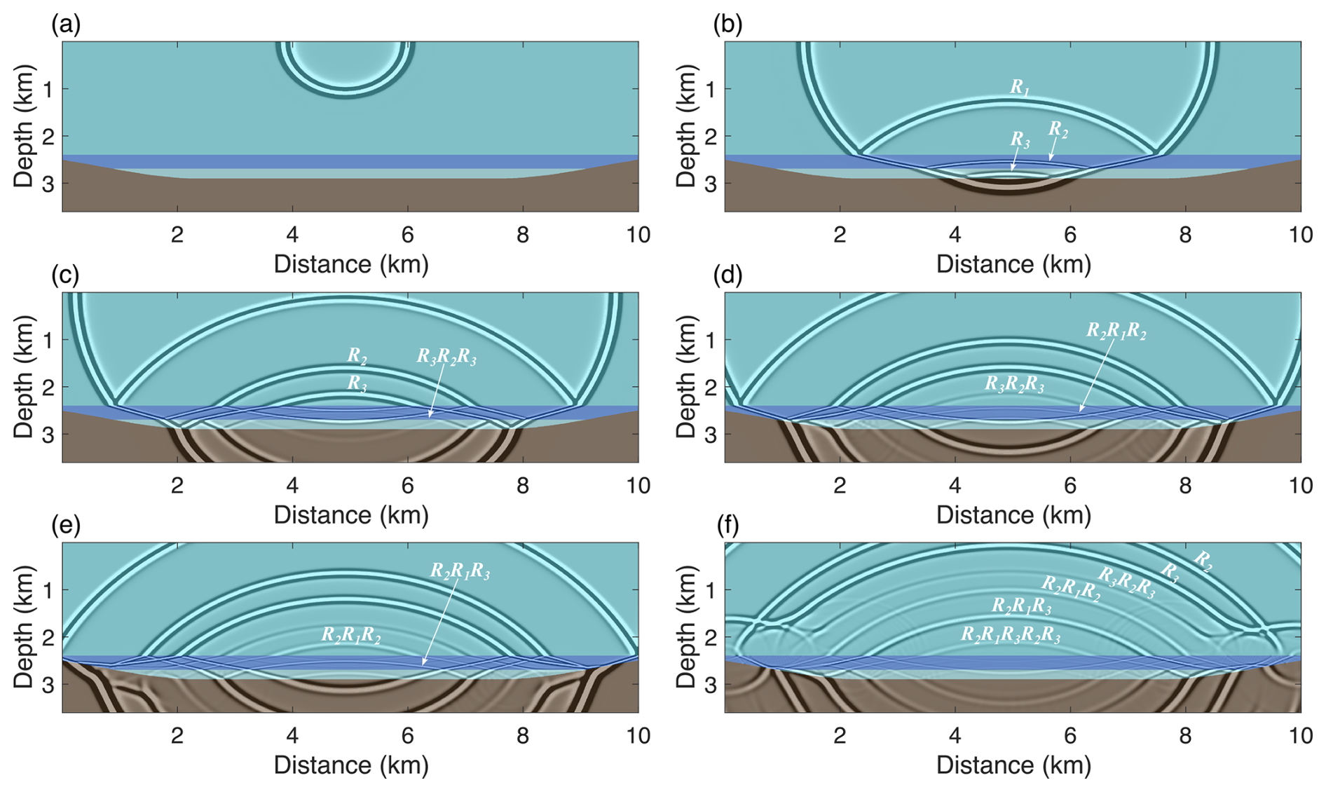
Figure 10 The wavefield snapshots at different time steps when a sediment layer is added at the bottom of the subglacial model, with (a) to (f) representing the wavefield snapshots at t=0.35, t=1.0, t=1.3, t=1.45, t=1.55, and t=1.85 s, respectively.

In the seismic records shown in Fig. 12e, reflections R₂ and R₃, along with the first-order interlayer multiples R₂R₁R₂ and R₃R₁R₂, as well as higher-order interlayer multiples, consistently appear in pairs. The time lag between seismic events within each pair is primarily influenced by the sediment layer thickness, while the time difference between pairs is governed by the water layer thickness. Furthermore, due to the low reflection coefficient at the sediment-bedrock interface, the amplitude of interlayer multiples within the sediment rapidly decreases with increasing order. In contrast, the amplitude of interlayer multiples within the water layer diminishes more gradually, due to the higher reflection coefficients at the ice-water and water-sediment interfaces.

2.6 Firn, sediment and free surface

Finally, we simulate the wavefield including the firn layer, the sediment layer, and the free surface, thereby constructing a model that closely represents realistic Antarctic subglacial conditions. As shown in Fig.11 the presence of the firn layer promotes guided-wave propagation in the near-surface region. The sediment layer gives rise to numerous interlayer multiples, propagating within the water layer, the sediment layer, or across both. The resulting wavefield closely resembles that in Fig. 10, with only minor variations in phase and amplitude attributable to the firn layer. The presence of the free surface causes upward-propagating reflected waves to be reflected back downward upon reaching the model surface. When these downward-propagating waves enter the water and sediment layers, they generate additional interlayer multiples, further complicating the wavefield.

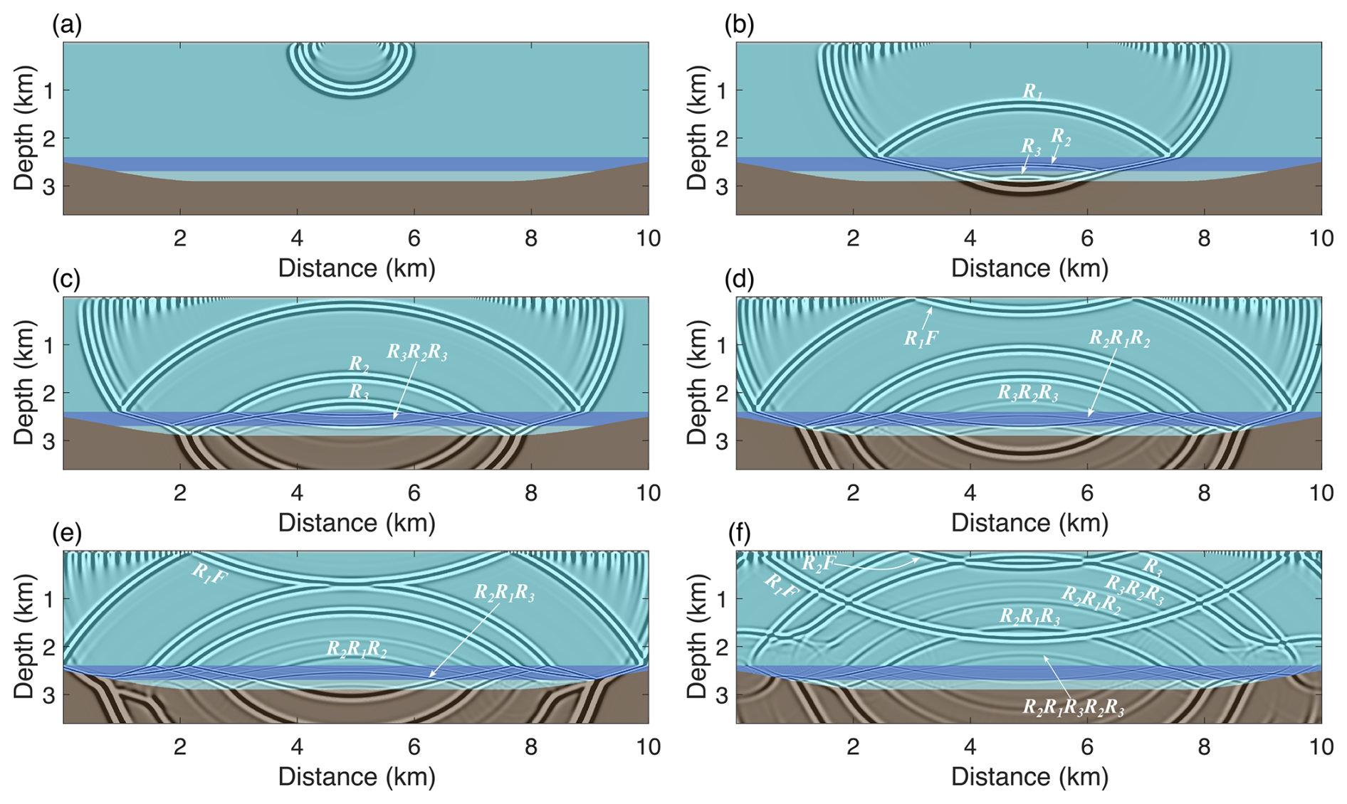
Figure 11 Wavefield snapshots at different time steps are shown for a model including the firn layer, sediment layer, and free surface. Panels (a)–(f) correspond to t=0.35, 1.0, 1.3, 1.45, 1.55, and 1.85 s, respectively.

2.7 Data comparison

The prestack shot gather from all six models are plotted together in Fig. 12, providing a clear comparison of the data differences under different modeling scenarios.

• With absorbing boundaries around the model, the seismic data show, in addition to the primary reflections R₁ and R₂ from the ice–water interface and lake bottom, first- and second-order interlayer multiples within the water layer (R₂R₁R₂ and R₂R₁R₂R₁R₂ in Fig. 12a). The time lag between these multiples and the primaries is mainly determined by the water-layer thickness.

• Applying a free-surface boundary condition at the model surface generates numerous free-surface multiples that are absent when an absorbing boundary condition is used (Fig. 12b), including first- and second-order free-surface multiples (R₁FR₁ and R₁FR₁FR₁) and hybrid multiples (R₂FR₁ and R₁FR₂) propagating across the ice sheet and water layer.

• When only the firn layer is added to the model, refracted waves appear in the wavefield compared to the absorbing-boundary simulation (Fig. 12c). The reduced velocity in the firn layer causes the direct-wave event to exhibit a steeper slope, as shown by the red dashed line.

• Compared with the free-surface-only case, the coexistence of the firn layer and free surface gives rise to pronounced guided wave in the red-boxed region of Fig. 12d, generated by refracted energy repeatedly interacting with the free surface.

• With a basal sediment layer present, the primary reflection R₃ arises from the sediment–bedrock interface, accompanied by numerous interlayer multiples that propagate within the sediment (such as R₃R₂R₃ in Fig. 12e), within the water layer, or across both, further complicating the subglacial wavefield.

• With the firn layer, sediment layer, and free surface, the seismic records display both guided waves and all reflections illustrated in Figure12e, along with free-surface multiples from the ice–water, water–sediment, and sediment–bedrock interfaces (e.g., R₁FR₁, R₂FR₂, R₃FR₃ in Fig. 12f).

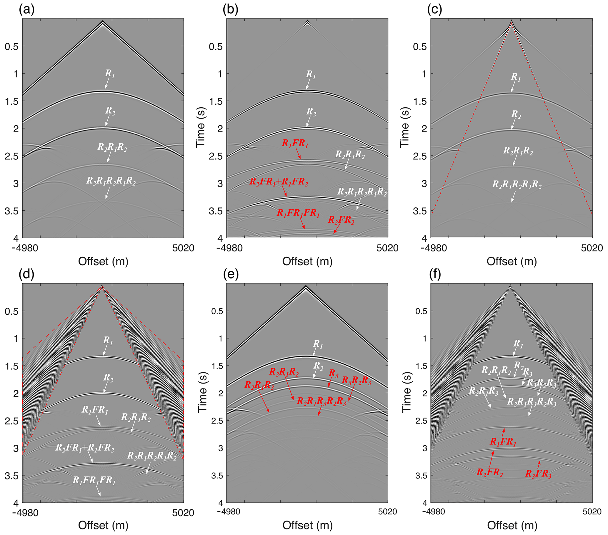
Figure 12 A common shot gather generated by the subglacial model, with (a) absorbing boundary, (b) free surface, (c) firn layer, (d) free surface + firn layer, (e) sediment layer and (f) free surface + firn + sediment layer.

Wavefield simulations and data comparisons indicate that the dominant features of subglacial lake seismic data are the pervasive occurrence of guided waves and multiples. Guided waves are, in essence, firn-layer multiples whose propagation is strongly controlled by firn structure, making them highly sensitive to variations in firn velocity and density. This sensitivity suggests that guided waves offer significant potential for high-resolution inversion of firn velocity and density profiles.

Both free-surface and interlayer multiples follow the primary reflections, with their time delays determined by the thicknesses and velocities of the ice sheet, water layer, and sediment. Only a subset of multiples is shown in Figure 12, due to the limited simulation time adopted in this study, longer records would capture higher-order multiples, although their amplitudes decrease rapidly with increasing order. Multiples can be both problematic and advantageous. Conventional seismic processing typically addresses only primary reflections, and misidentifying multiples as primaries introduces artifacts. However, because multiples undergo more reflections within the subglacial structure than primaries, they are more sensitive to velocity variations and offer significant potential for super-resolution imaging of subglacial structures.

3 Seismic data processing

Pre-stack seismic data acquired in the field cannot directly delineate subglacial geological structures. Accurate characterization of subglacial properties and architectures requires a sequence of data-processing procedures, including noise attenuation, static correction, velocity analysis, normal-moveout correction, stacking, and migration (Yilmaz, 2001). Based on the six geological models described above, we perform multi-shot forward simulations to produce the corresponding stacked sections, which serve as the basis for analyzing subglacial wavefield characteristics and structural features. In addition to the conventional seismic processing workflows, we also discuss in the following sections several methods and considerations specific to subglacial lake data, including strategies for subglacial lake imaging and factors influencing imaging accuracy.

3.1 Velocity analysis

We conduct 100-shot simulations with shot points spaced 100 m apart along the ice-sheet surface. Each shot gather comprises 500 traces with a receiver spacing of 20 m. Owing to the noise-free data and the flat surface of the model, neither denoising nor static correction is required. After velocity analysis, the common shot gathers (CSGs) are transformed into common midpoint (CMP) gathers, from which the velocity spectra are computed (Yilmaz, 2001). Figure 13 shows the velocity spectra for the CMP gathers at x=5 km for the six models, with stacking velocity on the horizontal axis and two-way travel time on the vertical axis. The energy clusters in the spectra result from coherently stacking reflection events along hyperbolic trajectories defined by the stacking velocity (Luo and Hale, 2012).

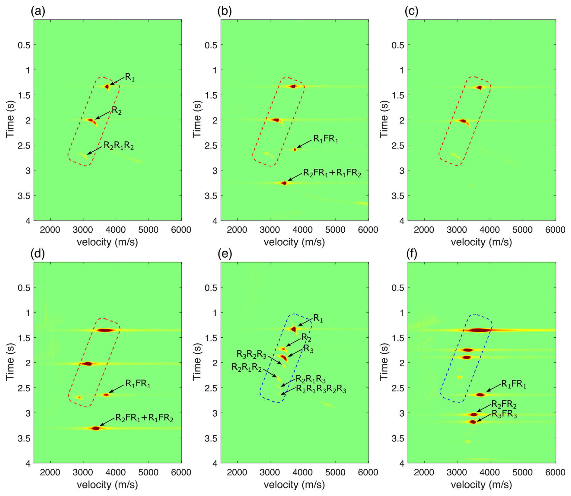
Figure 13 A velocity spectrum generated by the subglacial model, with (a) absorbing boundary, (b) free surface, (c) firn layer, (d) free surface + firn layer, (e) sediment layer and (f) free surface + firn + sediment layer.

The energy clusters in Fig. 13a represent, from top to bottom, the primary reflections R₁ and R₂ at the ice-water and water-bedrock interfaces, respectively, as well as the first-order interlayer multiple R₂R₁R₂ in the water layer. Due to the significantly lower velocity of water compared to glacial ice, the stacking velocity of R₂ is lower than that of R₁. Furthermore, as R₂R₁R₂ travels further within the water layer and is treated as a primary reflection during velocity analysis, its stacking velocity is also lower than that of R₂. Higher-order multiples within the water layer exhibit even lower stacking velocities, but these energy clusters are challenging to detect due to rapid amplitude attenuation after multiple reflections. Including the free surface in the model preserves the energy clusters observed in Fig. 13a (red dashed box) and introduces strong clusters associated with free-surface multiples. The stacking velocity of the first-order multiple (R₁FR₁) is close to that of the primary reflection R₁, whereas the first-order interlayer multiples (R₂FR₁ and R₁FR₂) exhibit lower stacking velocities.

Including a firn layer in the model generates refracted waves in the seismic data, while the combined presence of the firn layer and free surface gives rise to strong guided waves. However, because neither the refracted nor the guided waves in the CMP gathers follow hyperbolic trajectories, they contribute noise rather than coherent energy clusters to the velocity spectrum and must be removed before analysis. After their removal, the velocity spectra in Fig. 13c and d closely resemble those in Fig. 13a and b, except for a slight timing shift of the energy clusters caused by the firn layer.

Figure 13e shows the velocity spectrum for the model with a sediment layer beneath the subglacial lake. The primary reflections from the ice–water (R₁), water–sediment (R₂), and sediment–bedrock (R₃) interfaces appear as distinct energy clusters arranged from top to bottom. Below R₃, three weaker clusters emerge: the first-order multiples R₃R₂R₃ within the sediment layer, R₂R₁R₂ within the water layer, and R₂R₁R₃ propagating through both the water and sediment layers, all exhibiting lower stacking velocities than the primary reflections. Beyond these first-order multiples, a second-order interlayer multiple, R₂R₁R₃R₂R₃, appears with even lower amplitude due to its additional interlayer reflections. When the firn layer, free surface, and sediment layer coexist, the velocity spectrum (Fig. 13f) additionally contains first-order free-surface multiples R₁FR₁, R₂FR₂, and R₃FR₃ from the ice–water, water–sediment, and sediment–bedrock interfaces, respectively. Unlike the interlayer multiples, these free-surface multiples exhibit higher stacking velocities and stronger amplitudes.

3.2 Stacking

A stacking-velocity model is derived from the maximum-energy points of the clusters in each velocity spectrum and applied for normal moveout (NMO) correction. This flattens the reflections in the CMP gathers, which are subsequently stacked along the offset direction to yield the final image shown in Fig. 14.

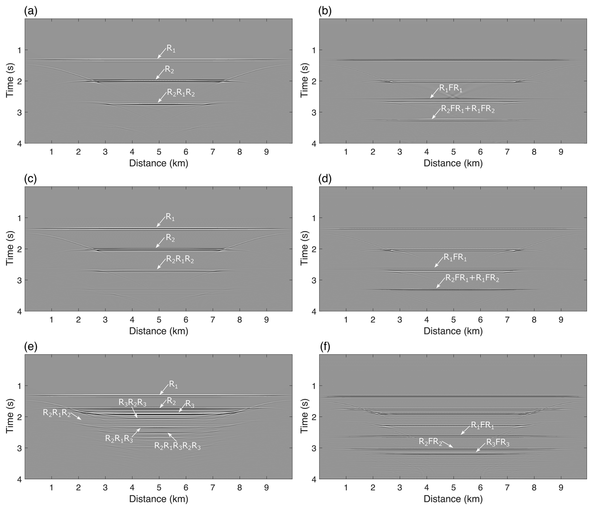
Figure 14 A stacked image of the subglacial model, with (a) absorbing boundary, (b) free surface, (c) firn layer, (d) free surface + firn layer, (e) sediment layer and (f) free surface + firn + sediment layer.

Figure 14a shows the stacked image of the model with absorbing boundaries. After NMO correction and stacking, the primary reflection R₁ appears as a horizontal event, indicating a flat ice–water interface, while R₂ forms a horizontal event near the center, corresponding to a flat lake bottom. Toward the model edges, R₂ inclines slightly, reflecting a gradual rise of the lake bottom. Below 2.5 s, additional reflection events appear, with widths and shapes similar to the lake-bottom, arising from the stacking of multiples R₁R₂R₁. When a free surface is introduced, free-surface multiples appear in the stacked section (Fig. 14b). The horizontal events at approximately 2.6 and 3.3 s correspond to the first-order free-surface multiple R₁FR₁ and a combined first-order interlayer multiple R₂FR₁+R₁FR₂, respectively, both partially capturing the characteristics of the ice–water interface and the lake bottom.

Figures 14c and d show the stacked sections for models with a firn layer alone and with both the firn layer and free surface, respectively, which closely resemble Fig. 14a and b. This similarity arises because the firn layer generates primarily refracted and guided waves rather than additional reflections. As these wave modes are not flattened by NMO correction, they fail to produce coherent events after stacking.

In the model with a sediment layer, the stacked image (Fig. 14e) clearly images the ice–water (R₁) and water–sediment (R₂) interfaces, as well as the sediment–bedrock interface (R₃). Below R₃, interlayer multiples generate additional coherent reflections. The first-order interlayer multiples R₃R₂R₃ and R₂R₁R₃ both align with R₃, with time shifts corresponding to propagation through the sediment and water layers, respectively. Beneath them, the second-order multiple R₂R₁R₃R₂R₃ produces another reflection aligned with R₃, corresponding to additional propagation through the sediment layer. Similarly, the first-order interlayer multiple R₂R₁R₂ aligns with the lake-bottom interface R₂, with a time shift corresponding to wave propagation through the water layer.

3.3 A robust approach for subglacial lake imaging

Accurate depth imaging of subglacial lakes requires a reliable velocity model. We propose a salt flooding–based workflow to construct such a model and thereby improve the fidelity of subglacial lake imaging. The imaging accuracy of the ice–water interface primarily depends on the velocity of the overlying ice sheet. With an accurate velocity, reflections along the interface coherently focus, yielding a high signal-to-noise ratio (SNR). Velocity errors, however, lead to defocused reflections, blurred interface imaging, and reduced SNR. To determine a reliable ice velocity, migrations were performed using a series of constant-velocity models, and the velocity producing the best interface imaging was selected. Figure 15a and b show migration results for velocities of 3700 and 3800 m s⁻¹, respectively. The latter yields a clearer interface with higher SNR, indicating an ice velocity of 3800 m s⁻¹.

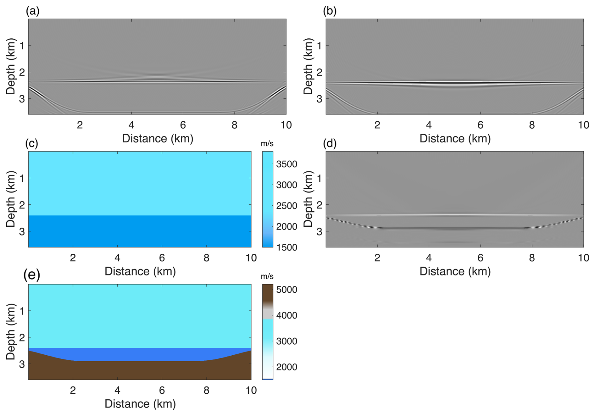
Figure 15 Workflow for constructing a reliable subglacial velocity model using the salt flooding method. (a, b) Migration results with constant velocities of 3700 and 3800 m s⁻¹, respectively. (c) Velocity model generated by the salt flooding method. (d) Migration image using the model in (c). (e) Final subglacial lake model obtained from the salt flooding workflow.

The imaging of the lake bottom also depends on the velocity and geometry of the water body. Because the lake morphology is unknown, the migration model assumes a uniform water layer beneath the ice–water interface. This approach, known as salt flooding, was originally developed for imaging high-velocity homogeneous media such as subsurface salt domes. The ice–water interface was then picked from the migrated section in Fig. 15b, and the velocity model was updated by assigning 1500 m s⁻¹ below the interface while retaining 3800 m s⁻¹ above, yielding the model shown in Fig. 15c. Migration with this updated velocity model produced the section shown in Fig. 15d, where the lake bottom is imaged at the correct depth with improved clarity. Similarly, the lake bottom was picked from the migrated section in Fig. 15d, and the velocity model was further updated by assigning a bedrock velocity below this horizon, resulting in the model shown in Fig. 15e.

3.4 Impact of Firn Layer on Subglacial Lake Imaging

Accurate determination of the ice–water interface depth is essential for subglacial lake drilling. If this depth is overestimated, the borehole may prematurely penetrate the lake, exposing the water directly to drilling equipment and fluids and risking contamination of its pristine, isolated environment. Conversely, if the interface lies deeper than expected, the drilling system may fail to reach the lake. In the planned Lake Qilin project, China will employ a combined strategy of rapid hot-water drilling followed by precision thermal drilling near the interface. Because the penetration capacity of the thermal drill is limited, an underestimated depth could trigger an early switch, preventing the drill from breaching the lake surface.

The accuracy of the firn velocity structure is critical for reliable imaging of the ice–water interface. Errors in the migration velocity distort traveltimes and systematically shift the interface. To demonstrate this effect, we performed forward modeling with the firn model shown in Fig. 5, and then migrated the synthetic data using a constant 3800 m s⁻¹ velocity model, both with and without explicit representation of the firn layer (Fig. 16a and b). As illustrated in Fig. 16c, neglecting the firn layer introduces artifacts in the interface image and produces a systematic depth bias: the migrated interface appears about 40 m deeper than its true position, marked by the blue dashed line.

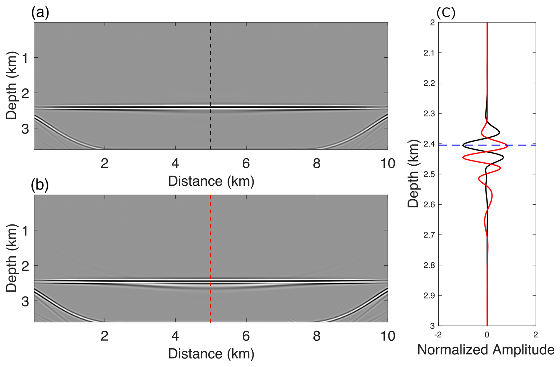
Figure 16 Migration results using a constant 3800 m s⁻¹ velocity model: (a) with and (b) without the firn layer. (c) Depth profiles at x=5 km, where black and red curves correspond to migrations with and without the firn layer, respectively. The blue dashed line denotes the true ice–water interface depth.

The Herglotz–Wiechert inversion (HWI) is a commonly used method for firn-layer seismic inversion (Hollmann et al., 2021). However, as a 1-D approach assuming a monotonic increase of firn density with depth, it may produce significant errors when lateral variations or shallow/deep velocity inversions occur. Given these limitations, firn-layer inversion should increasingly employ wave-equation–based methods, such as full waveform inversion (FWI), which avoid prior assumptions about the layer's structure and can more reliably reconstruct complex velocity models. Furthermore, the firn layer supports well-developed guided waves with multiple modes, suggesting that integrating guided-wave analysis with wave-equation inversion could enable super-resolution velocity reconstruction.

3.5 Effect of Seismic Source Depth on Subglacial Lake Imaging

Due to the highly porous nature of Antarctic firn, seismic waves tend to undergo considerable energy attenuation during propagation. To enhance energy transmission into the subsurface, seismic sources – typically explosives – are therefore usually placed at the bottom of boreholes several tens of meters deep rather than detonated at the surface. While this approach reduces seismic energy attenuation to some extent, it simultaneously introduces a new challenge: the generation of source-side ghosts. Source-side ghosts are generated when energy from a deeply emplaced seismic source propagates upward, reflects off the free surface, and then returns downward to interact with subsurface interfaces. Therefore, their occurrence mainly depends on the source depth rather than the source type. This phenomenon is more common in marine exploration, where sources (e.g., air guns) are typically deployed below the water surface. In seismic processing, if source-side ghosts are not suppressed, each subsurface interface appears as a pair of events in stacked and migrated sections. The upper event corresponds to the true reflection from the interface, revealing its position and structural features, while the lower event represents the ghost response, which can interfere with seismic interpretation.

To illustrate this phenomenon, we use the model introduced in Sect. 2.4 and simulate a shot fired at a depth of 40 m. The resulting common shot gather, shown in Fig. 17a, clearly displays the primary reflections R₁ and R₂ from the ice–water interface and lake bottom, respectively, each immediately followed by the corresponding source-side ghost reflections FR₁ and FR₂. Figure 17b and c (green solid lines) show the mechanism of these source-side ghost reflections, which are generated when part of the energy first propagates upward to the free surface and then reflects downward to the subsurface interfaces. The stacked and migrated sections are shown in Fig. 17d and f, respectively, with magnified views of the highlighted regions in Fig. 17e and g. The paired reflection events resulting from source-side ghosts can be clearly identified in these panels. These ghost reflections may interfere with the interpretation of subsurface structures and amplitudes, emphasizing the need for appropriate processing strategies – such as deghosting or modeling-based suppression – to ensure accurate imaging of the subglacial interfaces.

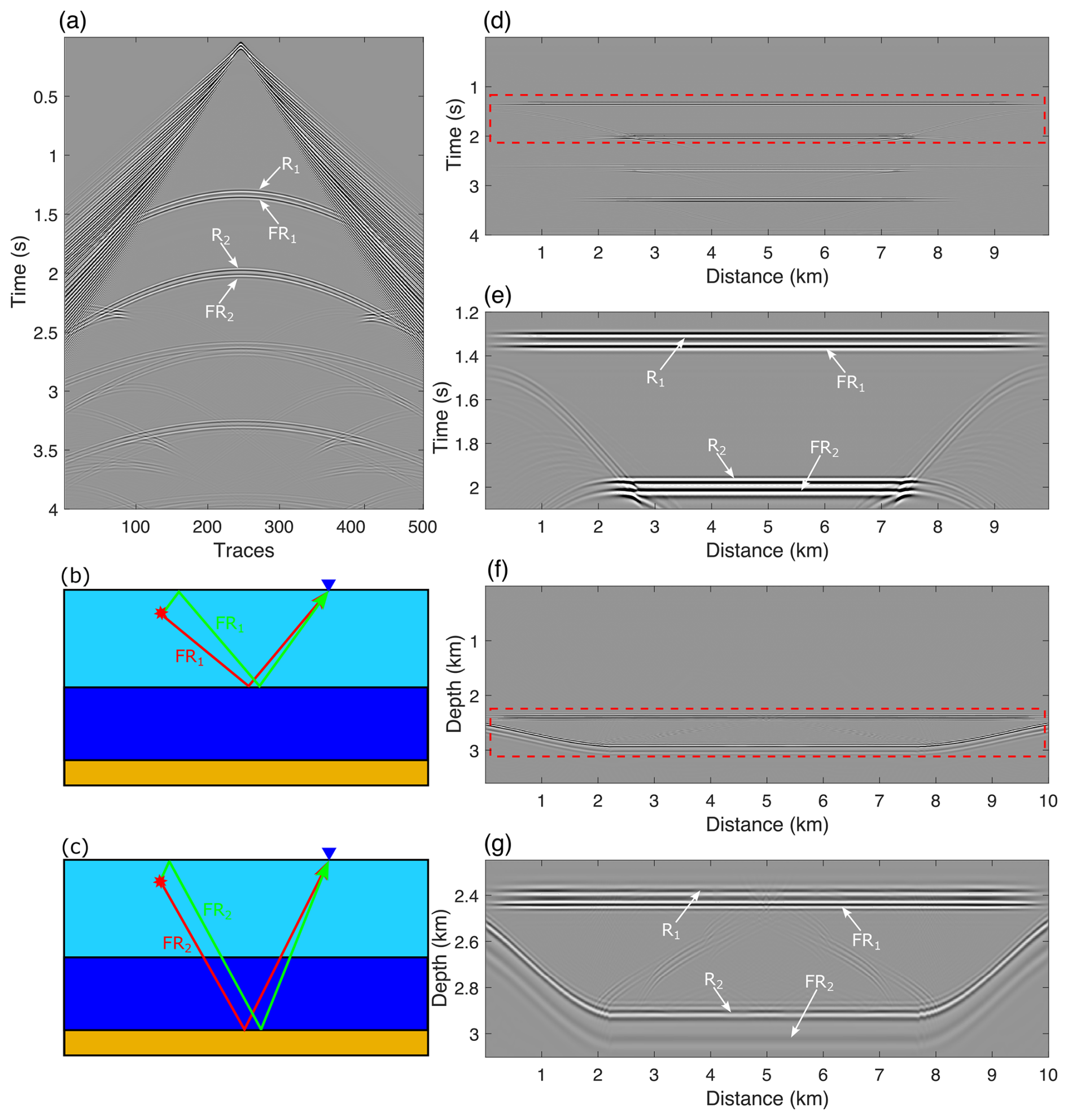
Figure 17 (a) A prestack common shot gather. (b–c) Ray-path analysis of reflections from the ice–water interface and the lakebed, including their associated source ghosts. (d) and (f) display the stacked and migrated sections, respectively, and (e) and (g) show zoomed in views of the highlighted areas in (d) and (f).

4 Seismic acquisition system

This section provides an overview of three commonly used active-source seismic systems in polar regions – leap-frog, snow-streamer, and full-coverage – by focusing on survey fold and coverage uniformity, which allows us to assess their impact on the quality and reliability of subglacial imaging.

4.1 Introduction of seismic acquisition in polar area

Figure 18 illustrates three active-source seismic acquisition systems: leap-frog (Clyne et al., 2020; McMahon and Lackie, 2006), snow-streamer (Eisen et al., 2015; Oetting et al., 2022), and full-coverage acquisition. Red stars and blue triangles denote shot and receiver locations, respectively. The leap-frog system, shown in Fig. 18a, usually employs a shorter receiver line with fewer receivers but larger offsets. Shot points are spaced at wide intervals along the receiver line, starting and ending away from the line edges. Once a sequence of shots is completed, the receiver line is advanced, and the process is repeated. The snow-streamer system, shown in Fig. 18b, typically uses a longer receiver line to achieve broader subsurface coverage. Shot points are positioned at a fixed offset ahead of the receiver line, and both advance together after each shot. This system often employs gimbal-mounted geophones (Van der Veen and Green, 1998), which move with the cable and do not require burial, making it well-suited for towed acquisition. In contrast, the full-coverage system, shown in Fig. 18c, deploys geophones across the entire survey area, with shots fired at fixed intervals along the receiver line. This approach generally requires a substantially larger number of geophones to achieve complete and uniform coverage.

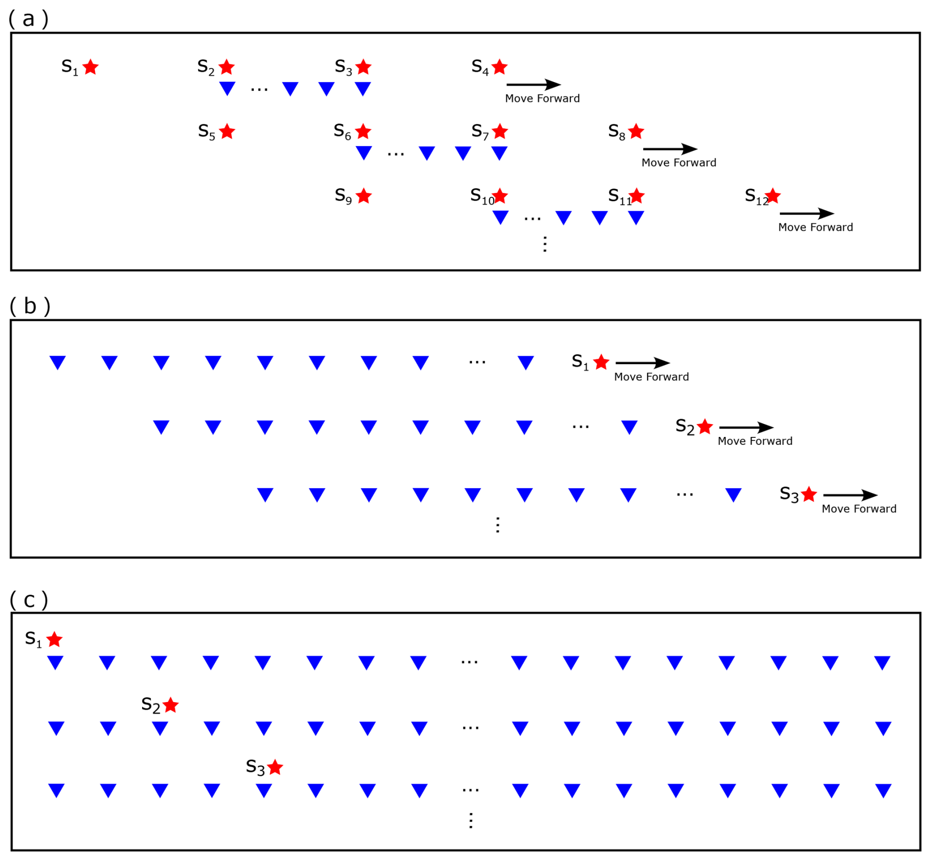
Figure 18 Comparisons of three active seismic data acquistion system, which are (a) leap-frog, (b) snow- streamer and full-coverage system.

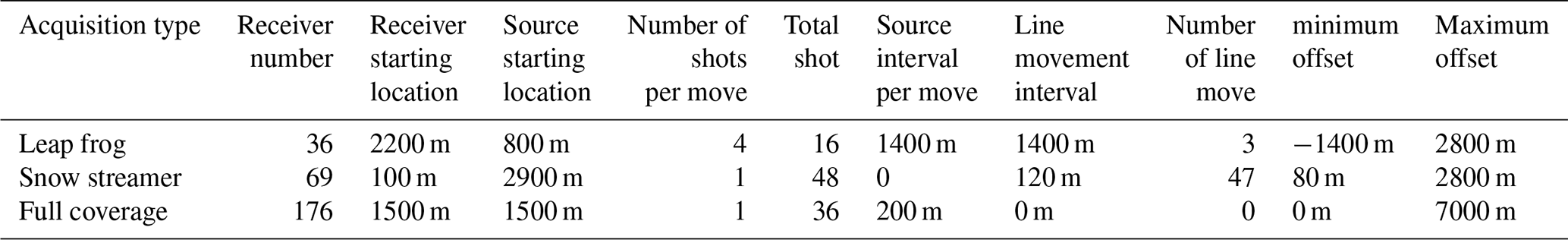
To compare the characteristics of the three acquisition systems, we simulated seismic surveys along a 10 km line for each system, with the specific parameters summarized in Table 2. Receiver spacing was set to 40 m, with survey coverage extending from x= 1500 to x=8500 m. The maximum offset was maintained at no less than 2.8 km, ensuring an offset-to-depth ratio of at least 1:1 (target depth 2.8 km), while the minimum offset was limited to 100 m. As shown in Table 2, the leap-frog system requires the fewest receivers, whereas the full-coverage system requires the most. Once deployed, the full-coverage array remains stationary throughout the survey, whereas the snow-streamer system requires the most frequent relocation. However, these acquisition parameters alone do not determine the actual field workload or operational challenges. In practice, factors such as the seismic-source type (e.g., vibroseis versus explosives), deployment methods for receivers and sources (surface-mounted versus buried), and local surface conditions (e.g., unconsolidated snow versus hard ice) and other factors also influence the practical effort and logistical demands of field acquisition. For example, although the snow-streamer system requires relatively more receivers and frequent line relocations (Table 2), its use in combination with gimbal-mounted geophones and a vibroseis source can achieve remarkably high acquisition efficiency. As reported by Smith et al. (2020), during the Ekström Ice Shelf survey, this configuration enabled a three-person team to acquire 20 km of seismic line in a single day.

Table 2 Acquisition parameters of the three seismic systems for a 10 km survey line.

4.2 Acquisition performance

Building on the above comparison, we next assess the three acquisition systems in terms of fold and coverage uniformity, which directly influence the final imaging quality. The fold is calculated by counting the number of source–receiver pairs that share the same midpoint, while the coverage uniformity is evaluated by analyzing the offset distribution of these midpoint bins. Figure 19 illustrates the coverage maps for the three acquisition systems. The leap-frog system exhibits the lowest fold because of its large shot spacing and wide line-movement intervals. In contrast, the snow-streamer and full-coverage systems, with their longer receiver lines and smaller shot intervals, achieve substantially higher fold than the leap-frog system. Among them, the snow-streamer system exhibits a more evenly distributed fold, whereas the full-coverage system shows a pyramid-shaped fold pattern, with coverage increasing linearly from the edges toward the center.

Figure 19 Fold coverage assesment of (a) leap-frog, (b) snow-streamer and (c) full-coverage acquisition system.

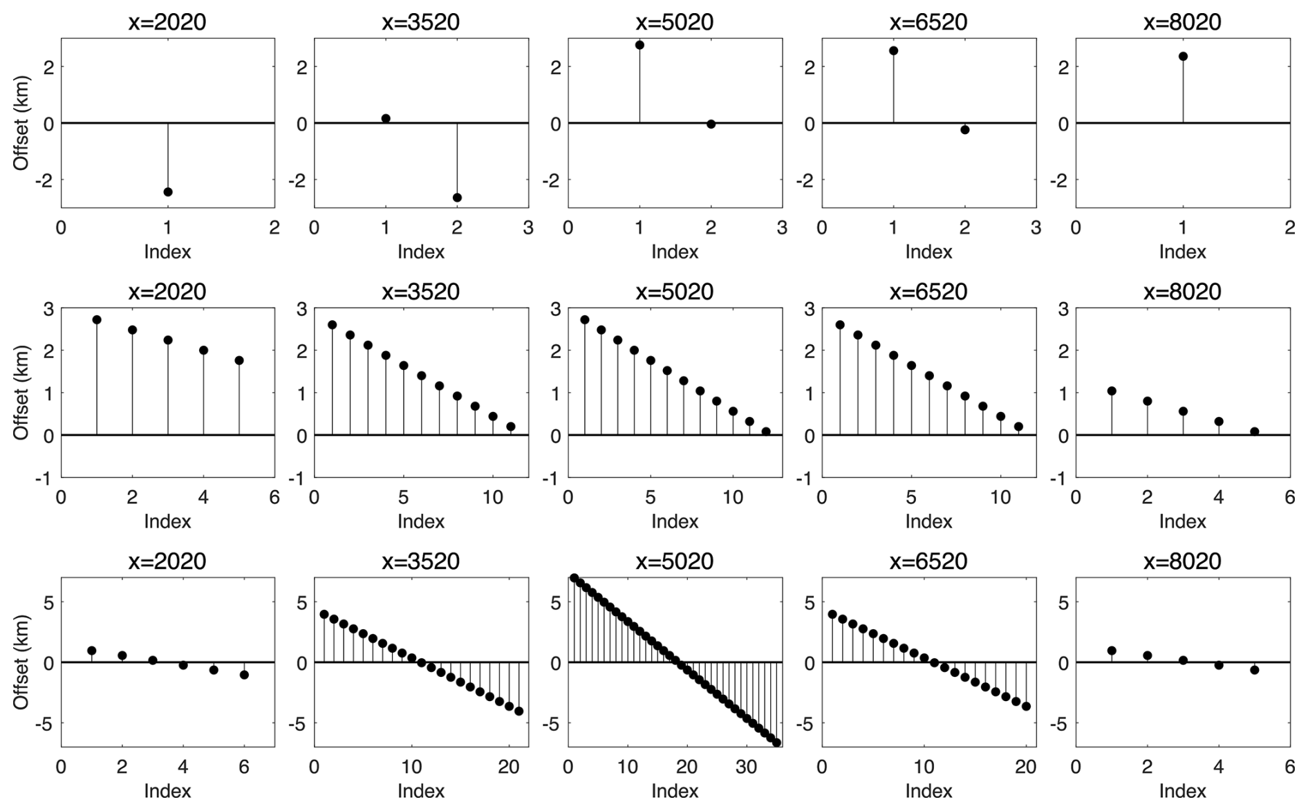
Figure 20 Coverage uniformity in a CMP gather of the (a) leap-frog, (b) snow-streamer, and (c) full-coverage acquisition systems.

Figure 20 shows the coverage uniformity of the three acquisition systems. In the leap-frog system, each midpoint has both low fold and highly variable source–receiver offsets, which can lead to two issues: (1) for pre-stack data with low signal-to-noise ratio, stacking fails to sufficiently enhance the SNR; and (2) reliable amplitude-versus-offset (AVO) information is difficult to obtain, limiting the characterization of rock properties across interfaces (Buland and Omre, 2003; Peters et al., 2008). By contrast, the snow-streamer and full-coverage systems achieve higher and more uniform fold with a broader range of offsets. The snow-streamer samples only positive offsets due to its single-sided shooting, whereas the full-coverage system provides a symmetric distribution; overall, both systems ensure more reliable imaging and AVO analysis.

We have reviewed three commonly used active seismic acquisition systems in polar regions and highlighted their main characteristics. The leap-frog system provides an effective way to achieve full survey coverage when the number of receivers is limited, although it results in low fold. The snow-streamer system requires frequent relocation of receivers and shot points, but with gimbal-mounted geophones and vibroseis sources it achieves high efficiency, though it generally cannot record three-component data. When sufficient receivers are available, the full-coverage system is a suitable choice, providing higher fold, wider offset ranges, and a more symmetric and uniform offset distribution, which can benefit seismic migration, inversion, and pre-stack analyses such as AVO.

The above comparison highlights the characteristics of each acquisition system but does not identify a universally “best” choice. In practice, survey feasibility depends on multiple factors beyond survey fold and coverage uniformity, including environmental conditions, logistical constraints, source and receiver types (e.g., explosive versus vibroseis sources), deployment strategies (e.g., surface placement versus buried installation), and other field-specific considerations. Consequently, selecting an acquisition system requires a case-by-case assessment to ensure practical and effective implementation under the prevailing conditions.

5 Lago Subglacial CECs Seismic Data Analysis

To validate the above conclusions, we reprocessed and analyzed seismic data acquired over Lago Subglacial CECs (SLC) (Rivera et al., 2015). These data, originally reported by Brisbourne et al. (2023b), were collected along four active-source seismic reflection lines across the lake. The survey employed a leap-frog deployment strategy (Fig. 21a), in which receivers and sources were alternately advanced along the profile. The receiver array comprised two 24-channel strings of geophones spaced at 10 m and buried at a depth of 40 cm. Sources were fired at 240 m intervals. After each round of shots, the source line was shifted forward by 240 m, while one receiver cable was leap-frogged past the other and redeployed. Explosive sources – three pentolite boosters totaling 175–400 g – were detonated in boreholes approximately 20 m deep. As indicated by the fold and offset distributions (Fig. 21b, c), each midpoint along the line was sampled by a single trace with a fixed offset. This geometry enables rapid full-line coverage but, lacking fold stacking, limits the ability to enhance signal quality during processing. This limitation becomes particularly acute when the acquired data have low signal-to-noise ratios.

Figure 21 (a) Acquisition geometry of the CEC seismic line (e.g., Line A), with red stars denoting source positions and green dots indicating receiver locations. (b) Fold coverage of the survey. (c) Uniformity of offset distribution.

The seismic data were recorded for 4.096 s with a sampling interval of 0.125 ms. Figure 22a shows a common shot gather (CSG) acquired near the center of Line A. Strong guided waves are observed in the shallow time region, consistent with the firn-layer simulations in Sect. 2.4. Distinct primary reflections from the ice–bedrock interface (R₁) and the lake bottom (R₂) appear within the green and yellow dashed boxes, with R₂ exhibiting reversed polarity relative to R₁. The blue dashed box highlights the first-order interbed multiple R₂R₁R₂ within the water layer, whose polarity matches R₁. Due to the extra reflection in the water layer, it arrives roughly one R₂–R₁ interval after R₂, a lag primarily governed by water-layer thickness. The purple dashed box indicates the first-order free-surface multiple of the ice–water reflection propagating within the ice sheet (mechanism in Sect. 2.2). Its arrival time is approximately twice that of R₁, with polarity identical to R₁ and lag determined by ice-sheet thickness. The orange dashed box marks the first-order free-surface multiple reflecting successively from the ice–water interface and lake bottom. Its polarity is opposite to that of R₁FR₁, arriving roughly one two-way water-layer travel time after R₁FR₁. Notably, each of these reflections is immediately followed by a counterpart with identical slope but opposite polarity, representing the source-side ghost caused by the relatively deep source burial. Figure 22b–g present enlarged views of the reflections highlighted by the red, green, yellow, blue, purple, and orange dashed boxes in (a), while Fig. 22h–m show the corresponding ray-path analyses for these reflections.

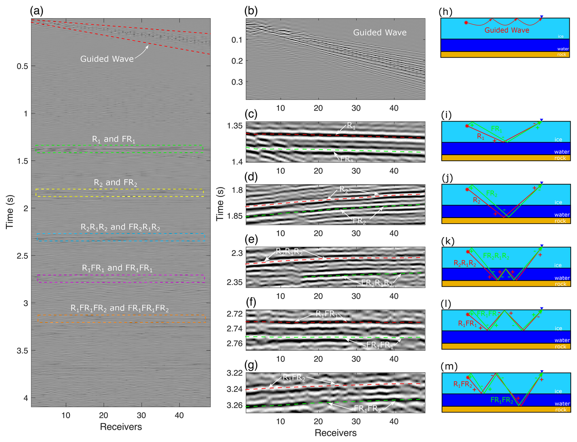
Figure 22 (a) A single-shot seismic record acquired at the central part of Line A, showing prominent guided waves and multiple reflections. (b–g) Enlarged views of the red, green, yellow, blue, purple, and orange dashed boxes in (a), highlighting: (b) guided waves; (c) the primary ice–water reflection R₁ and its source-side ghost FR₁; (d) the primary lake-bed reflection R₂ and corresponding ghost FR₂; (e) the first-order water-layer internal multiple R₂R₁R₂ and its ghost FR₂R₁R₂; (f) the first-order free-surface multiple of the ice–water interface R₁FR₁ and its ghost FR₁FR₁; and (g) the free-surface multiple R₁FR₂ and its ghost FR₁FR₂. (h–m) Ray-path diagrams corresponding to the wave types highlighted in panels (b)–(g).

The seismic data were NMO-corrected using velocities of 3800 m s⁻¹ for ice–water and 3650 m s⁻¹ for lake-bottom reflections, then stacked to produce the sections shown in Fig. 23a–d for Lines A–D. Figure 24a–d present zoomed-in views: the first-column panels correspond to the red dashed boxes in Fig. 23a–d, while the second-column panels focus on the ice–water and lake-bottom interfaces. These stacked sections provide a well-resolved preliminary view of the ice–water and lake-bottom structures. However, several steeply dipping reflectors, visible in Fig. 23, intersect the ice–water and lake-bottom reflections. These off-line reflections, likely originating from the inclined margins of the subglacial lake, cannot be correctly repositioned by stacking, partially obscuring the true morphology of the lake boundaries. In addition, primary and multiple reflections observed in the common shot gather (Fig. 22) are better resolved in the stacked sections, with different reflection types indicated by white arrows in Fig. 23. The combination of mispositioned reflections and stacked multiples generates spurious structures that may obscure the true geology and complicate interpretation.

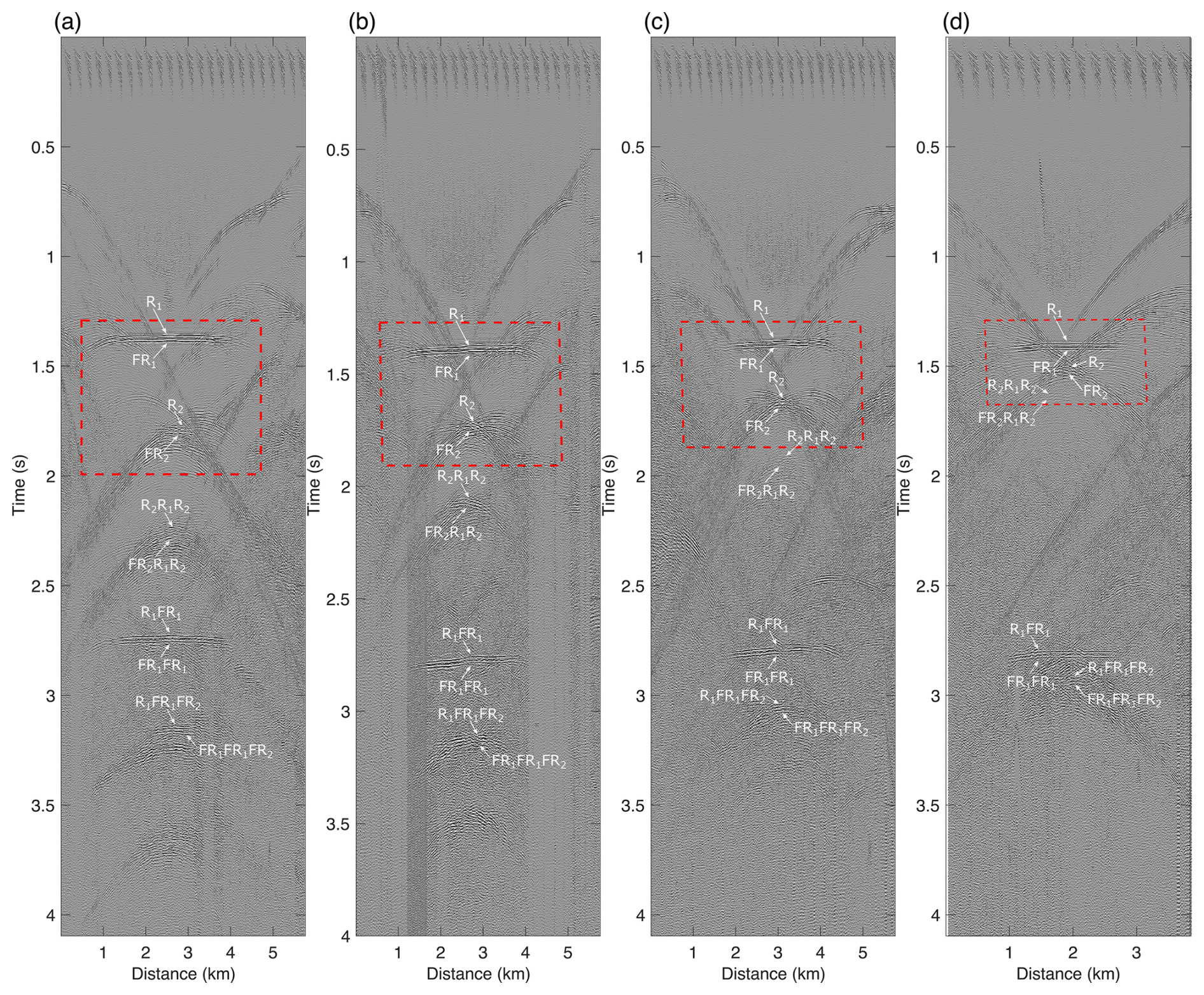
Figure 23 (a–d) Stacked seismic reflection profiles along Lines A, B, C, and D, respectively.

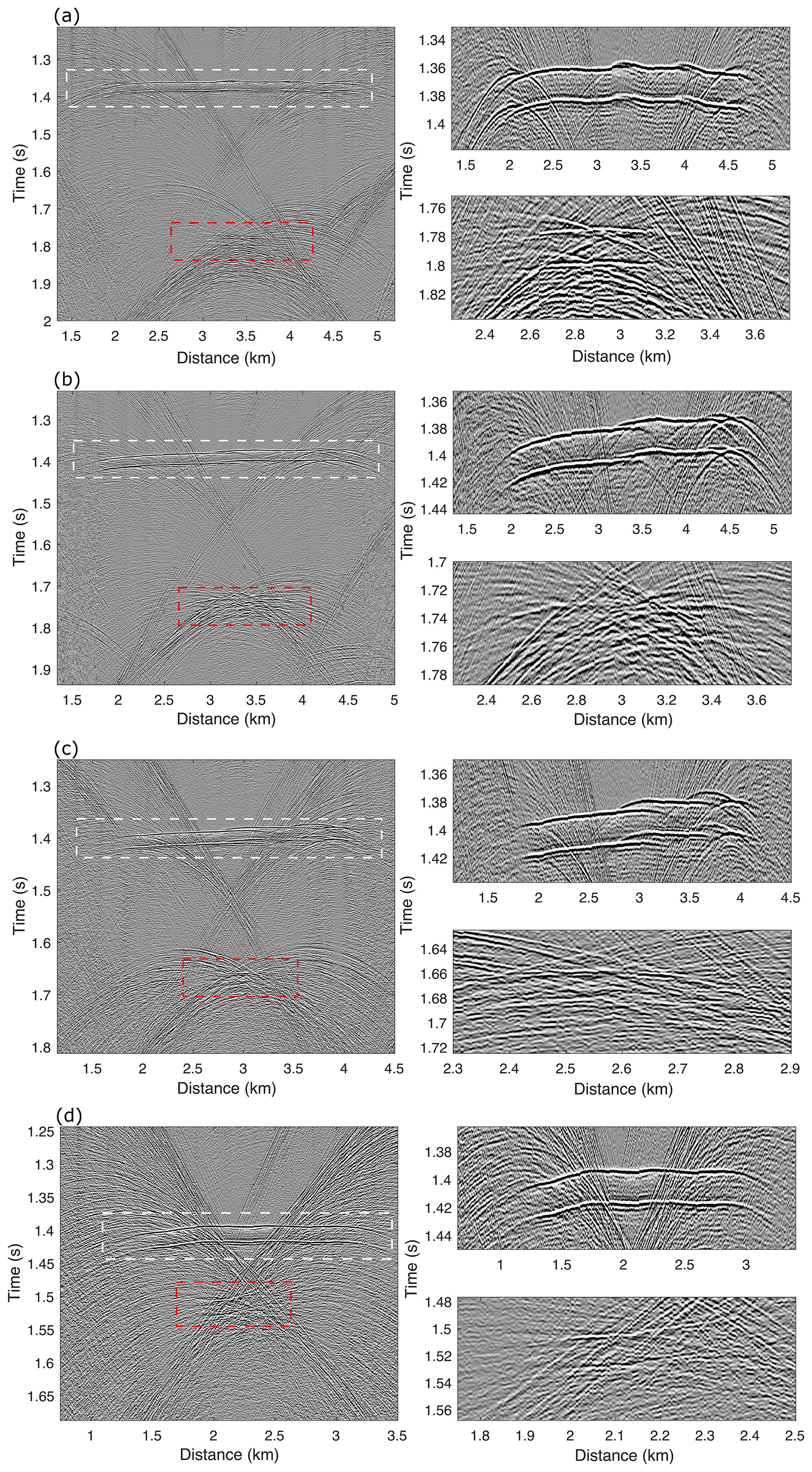
Figure 24 The first-column panels of (a)–(d) present magnified views of the red-dashed boxes in Fig. 23a–d, respectively. The second-column panels further enlarge the ice–water interface (white-dashed boxes) and the lake-bottom (red-dashed boxes) highlighted in the corresponding first-column panels.

We applied the salt-flooding strategy described in Section 3.3 to migrate the seismic data from Lines A–D. (1) RTM was first performed on the prestack data using a constant velocity of 3800 m s⁻¹ to delineate the ice–water interface. (2) The picked interface was then used to update the velocity model by assigning a velocity of 1500 m s⁻¹ below the ice–water interface. (3) RTM was repeated with the updated model to generate the migration images for Lines A–D (Fig. 25a–d) . These migration results accurately depict the morphology of the CEC subglacial lake and clearly resolve the structural boundaries along its flanks. The ice–water interface deepens from ∼ 2558 m on Line A to ∼ 2622 m on Line D, indicating a progressive northwestward deepening of the lake. Meanwhile, the interface narrows from ∼ 2704 m on Line A to ∼ 1585 m on Line D, reflecting a progressive northwestward narrowing. Further, the migration images in Fig. 26 show that the water column thickness decreases from ∼ 330 m on Line A to ∼ 98 m on Line D, indicating a progressive northwestward thinning of the lake. It should be noted that reflectors in the migration sections consistently appear in pairs due to the imaging of source-side ghost events.

Figure 25 (a–d) RTM-migrated images along Lines A, B, C, and D, respectively.

Figure 26 (a–d) Enlarged views of the red-boxed areas in Fig. 25a–d, respectively.

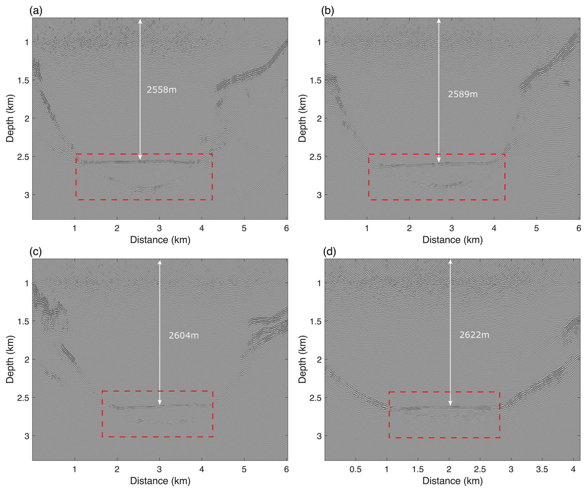
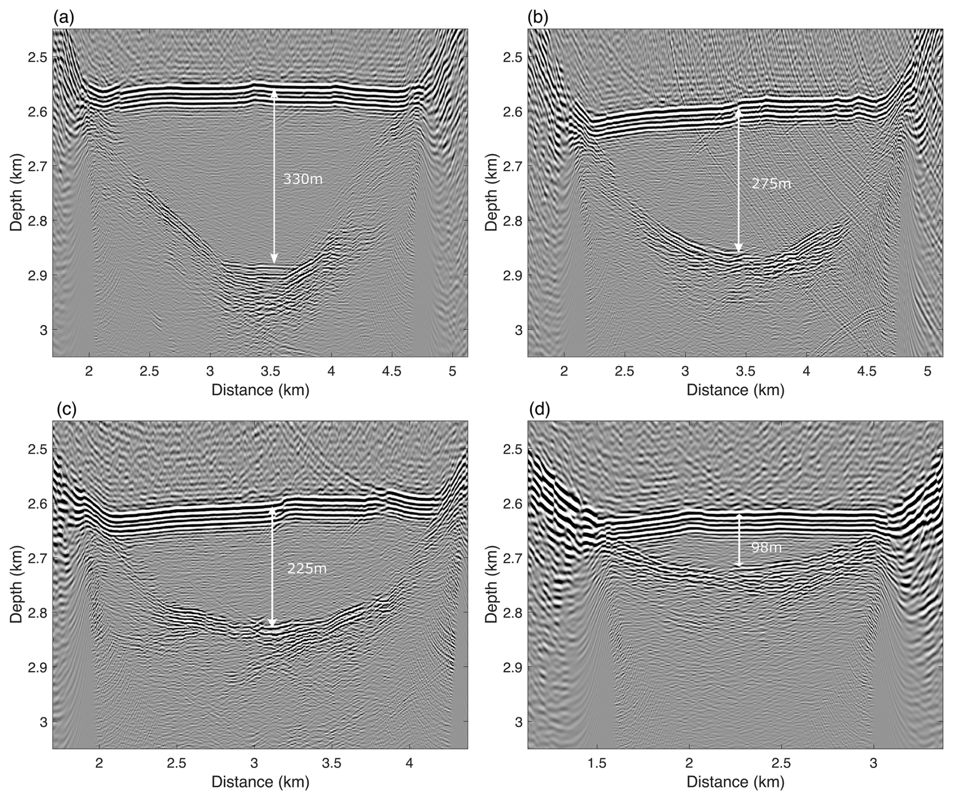
Apart from the lake’s overall geometry, the migration profiles also reveal relatively steep flanks on both sides of the lake. However, due to the limited fold and migration aperture, some of these steeply dipping interfaces are poorly imaged. Moreover, isolated reflectors appear on both flanks of the lake, which are likely caused by out-of-line reflections. The migration images indicate that the CEC subglacial lake occupies only a fraction of a deep U-shaped trough, with the water column representing roughly one-quarter to one-third of the total depression depth. The reasons behind this limited water-column thickness relative to the trough depth remain unclear and warrant further investigation using complementary approaches

6 Conclusions

Active-source seismic exploration of subglacial lakes has a long history, yet studies on their seismic wavefield characteristics remain scarce. In this study, we construct a representative subglacial lake model to analyze seismic responses, explore key processing challenges, and review commonly used acquisition systems in polar regions. Beyond its relevance to the seismic exploration of Lake Qilin, this study offers theoretical insights applicable to broader subglacial lake investigations.

This study first examines four aspects – wavefield simulations, pre-stack data comparisons, velocity spectrum analyses, and stacked section comparisons – to identify two dominant features: (1) the widespread occurrence of multiples within and across ice, water, and sediment layers, and (2) the pronounced development of guided waves in the near-surface firn layer. The observed multiples are primarily interlayer and free-surface types. Interlayer multiples, propagating mainly within the water and sediment layers, exhibit lower stacking velocities and generally arrive shortly after the primary events, with time delays controlled by water depth and sediment thickness and velocity. Free-surface multiples propagate predominantly within the ice, with arrival times determined by ice thickness and velocity; due to the typically greater thickness of Antarctic ice, these multiples appear later in the seismic records. Multiples occur in successive orders, with amplitudes decaying rapidly as order increases.

In conventional seismic processing, workflows are primarily optimized for primary reflections, with multiples and guided waves generally treated as noise. If not properly suppressed, these waveforms can generate spurious events in stacked and migrated images and degrade the overall signal-to-noise ratio. Techniques such as predictive deconvolution (Sun et al., 2014), surface-related multiple elimination (SRME) (Verschuur et al., 1992), and Radon-transform–based approaches (Liu et al., 2012) are widely employed to attenuate free-surface and interlayer multiples. Adapting these methods to subglacial lake settings may provide an effective means of enhancing seismic imaging quality. Beyond suppression, multiples also hold great potential for super-resolution imaging. While the theoretical resolution limit for primary reflections is approximately $\mathit{\lambda }/\mathrm{4}$, multiples – owing to their sensitivity to small-scale subsurface heterogeneities – can achieve resolutions approaching $\mathit{\lambda }/\mathrm{8}$ or better. Accordingly, developing multiple-based imaging techniques may enable super-resolution characterization of subglacial lake structures.Guided waves exhibit similar potential. As they result from repeated reflections near the free surface, they are highly sensitive to subtle velocity variations within the firn layer. Moreover, their pronounced dispersion characteristics make them well suited for reconstructing high-resolution velocity models of the near-surface firn. Building on conventional processing challenges, we further introduced a salt flooding approach tailored for subglacial lake imaging, assessed the effect of firn layers on ice–water interface resolution, and analyzed the mechanisms of source-side ghosts commonly observed in Antarctic seismic data. Together, these results provide both theoretical insights and practical guidance for advancing seismic investigations of subglacial lakes.

Next, we summarized several commonly used seismic acquisition systems in Antarctica: leap-frog, snow-streamer, and full-coverage, and compared them in terms of fold and coverage uniformity. The leap-frog approach enables rapid full-line coverage with a minimal number of receivers, though its fold remains relatively low. Snow-streamer surveys involve more frequent line relocations but can achieve high efficiency when paired with gimbal-mounted geophones and vibroseis sources, but typically cannot record three-component data. Full-coverage arrays are feasible when sufficient receivers are available. Once deployed, they remain fixed, simplifying field operations. It should be noted that no acquisition system can be deemed universally optimal. Survey feasibility depends on factors beyond fold and coverage, including environmental conditions, logistical constraints, source and receiver types (e.g., explosive or vibroseis), deployment strategies (e.g., surface versus buried), and other field-specific considerations. Selection must therefore be made on a case-by-case basis to ensure effective implementation under prevailing conditions.

Finally, we analyzed and processed the 2D active-source seismic data acquired over Lago Subglacial CECs (SLC). The data clearly reveal interlayer and free-surface multiples, source-side ghosts, and guided waves, consistent with the features identified in first Section. After stacking and migration using the salt flooding technique, the energy of multiples and ghosts persists in the images. These spurious events mimic the shape of primary reflections but appear at deeper depths, corroborating the observations from Sect. 3.2. Moreover, due to the use of the leap-frog acquisition system, the maximum fold is only 1, which likely contributes to the poor imaging of steep interfaces on either side of the lake. Migrated sections further indicate that the ice–water interface deepens from southeast to northwest (∼ 2558 m on Line A to ∼ 2622 m on Line D), while the lake narrows (∼ 2704 m on Line A to ∼ 1585 m on Line D), and water depth decreases from ∼ 330 to ∼ 98 m along the same trend.

For simplicity, this study adopts the acoustic wave equation. To capture a more complete wavefield, however, additional physical factors could be incorporated. For instance, firn porosity and meltwater may attenuate seismic waves, which could be addressed using a viscous wave equation (Hao and Greenhalgh, 2019; Agnew et al., 2023; Picotti et al., 2024). Shear wave propagation through the ice sheet and bedrock suggests the potential application of an elastic wave equation (Virieux, 1986), while the ice sheet’s layered anisotropy may also influence wave behavior (Alkhalifah, 2000; Llorens et al., 2020). These extensions will be explored in future work, with simulation results validated against active-source seismic data from Lake Qilin.