A new coastal ice-core site identified in Dronning Maud Land, Antarctica, for high-resolution climate reconstructions to the Last Glacial Maximum

High-resolution ice cores from the Antarctic Ice Sheet margin are crucial for reconstructing the climate history of Antarctica and the Southern Ocean. Ice-rise summits with stable positions and substantial snow accumulation can be ideal sites for such ice cores. We surveyed two ice rises at 16° E, at the eastern edge of the Lazarev Ice Shelf. Kupol Verbljud (VER) is an isle at the calving front, and Kamelryggen (KAM) is a promontory landward of VER. The radar survey reveals ice thicknesses of 560 m under VER's summit and 525 m under KAM's summit. The long-term stable englacial features, Raymond Arches, are observed in both ice rises, but while VER's arches are tilted, KAM exhibits vertically-aligned arches within its summit, indicating a more stable summit position. We find KAM's summit area is better suited for a long ice core, given its gentler bed slope and simpler ice stratigraphy. Surface mass balance derived from dated internal reflection horizon show consistent spatial patterns over recent decades. Using a one-dimensional age-depth model we consider the local ice flow as a combination of two extreme cases: diverging divide flow and shear-dominated flank flow. We determine which combination of these flow regimes best reproduces the mapped englacial radar stratigraphy and use it to estimate the age of ice. We conclude that KAM's summit is well-suited for obtaining a high-resolution ice core record beyond the Last Glacial Maximum with expected ∼20 ka-old ice at a depth 80 m above the bed where the resolution is expected to be 2.5 a cm⁻¹.

1 Introduction

Antarctica has experienced several significant climatic events since the Last Glacial Maximum (LGM; 20 ka). These events, such as the Last Deglaciation (18–11 ka; Mayewski et al., 1996), the Antarctic Cold Reversal (14.7–13 ka; Pedro et al., 2016), and the abrupt cooling event 8.2 ka ago (Stager and Mayewski, 1997), often display characteristics that contrast with those observed in comparable Northern Hemisphere events (Pedro et al., 2011; Burroughs, 2003). For example, the Antarctic Cold Reversal coincided with the warm Bølling-Allerød period in the Northern Hemisphere, while the impact of the 8.2 ka cooling event was less pronounced in the Southern Hemisphere than in the Northern Hemisphere (Wiersma and Renssen, 2006). The causes underlying these climate contrasts between the two hemispheres remain unclear. These climatic events manifest primarily as changes in temperature and sea level. As Antarctica's low-elevation coastal regions are at the forefront of these changes, they are ideal locations to study the southern polar climate and gain valuable insights into their connection to the global climate.

The coast of Dronning Maud Land (DML) faces the Atlantic sector of the Southern Ocean, which is characterized by the Weddle Gyre and its strong connections between the ice sheet, the atmosphere, and the global ocean circulation through its deep waters. The Atlantic meridional circulation couples climate changes in the Northern Hemisphere to this sector of the Southern Ocean (Rahmstorf, 2006). As a pivotal component of the larger carbon cycle, this region significantly influences global climate patterns over timescales ranging from centuries to millennia (Vernet et al., 2019). Despite its importance, there is a lack of continuous millennia-scale, high-resolution climate records from the coast of DML.

Ice core records from the DML coast (elevation below 2000 m a.s.l.) have been used to reconstruct surface mass balance (SMB) (Thomas et al., 2017; Philippe et al., 2016; Vega et al., 2016; Schlosser et al., 2014; Kaczmarska et al., 2004), temperature (Ejaz et al., 2022; Naik et al., 2010; Divine et al., 2009), melt chronology (Dey, 2023; Kaczmarska et al., 2006), sea ice variability (Ejaz et al., 2021), dust influx (Laluraj et al., 2020) and other climate variables at an annual to decadal timescale. The high resolution of the retrieved records is ensured due to the high surface mass balance across the coast of DML (Vega et al., 2016; Philippe et al., 2016; Schlosser, 1999). However, since these cores are limited to less than three centuries (Thomas et al., 2017), there is a need to retrieve longer ice cores from this region.

To identify an ideal site for an ice core record in coastal DML, we used five criteria: (I) a simple ice-flow regime to avoid ice-dynamical complexities in the ice core data; (II) minimal or no surface melting, as melting can potentially affect the distribution of water isotopes and trace element chemistry within the ice core; (III) sufficiently old ice, at least 20 000 years or older; at (IV) sufficiently high resolution to allow for annual layer counting, and (V) proximity to a logistics support hub, in our case the Indian Maitri Station in central DML (12° E, Fig. 1a). These criteria increase the likelihood of obtaining a high-resolution ice core that captures valuable climate information.

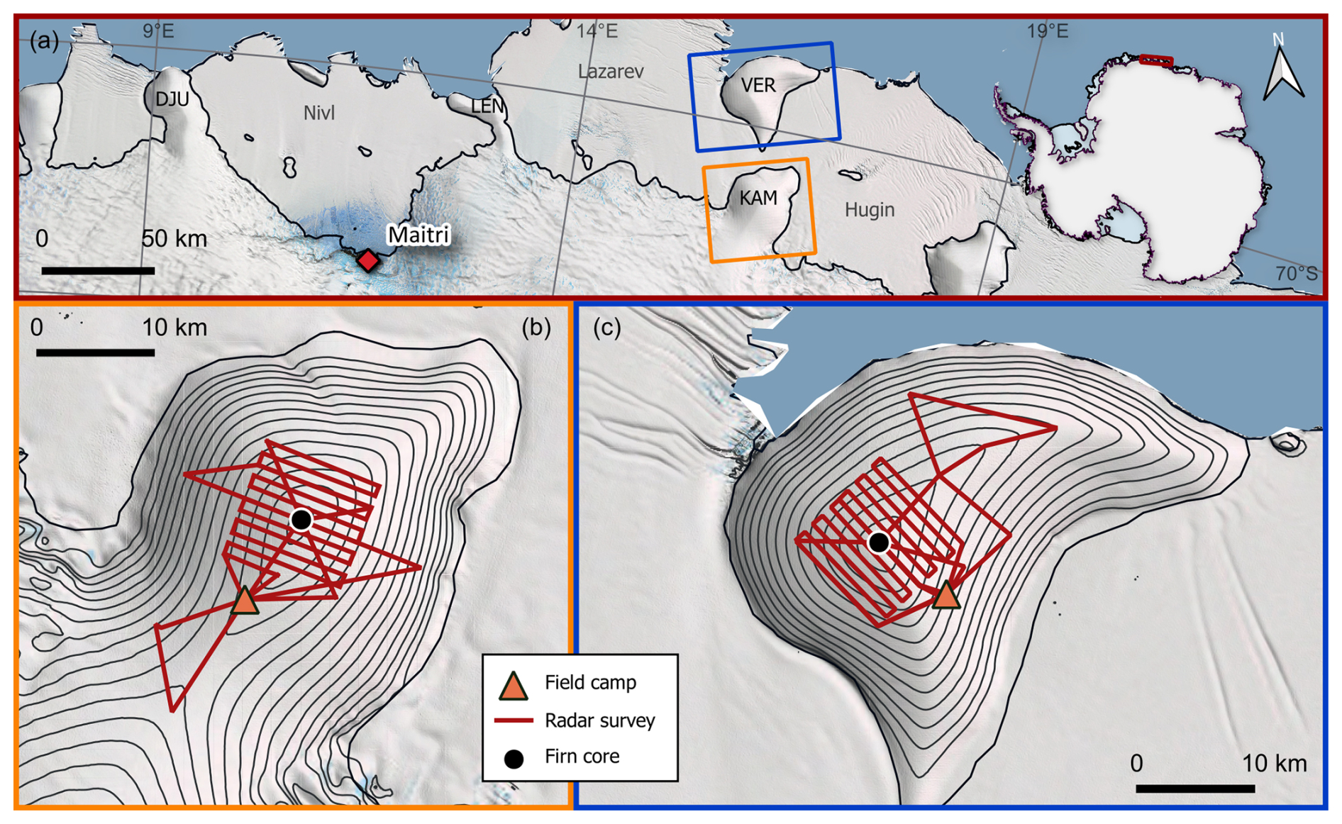
Figure 1 Kamelryggen (KAM) and Kupol Verbljud (VER) Ice Rises, east of the Lazarev Ice Shelf, central Dronning Maud Land (DML), East Antarctica. (a) Location of KAM and VER with black curves showing the ice sheet and ice rise grounding lines. DJU stands for Djupranen Ice Rise, and LEN stands for Leningradkollen Ice Rise. The grey text shows the names of the ice shelves. The inset shows the map coverage. The orange box over KAM shows the extent of (b), and the blue box over VER shows the extent of (c). (b–c) the zoomed-in view of ice rises with radar and firn core locations marked. The background is Landsat Image Mosaic of Antarctica (Bindschadler et al., 2008). Surface topography is shown with 20 m interval contours using the Reference Elevation Map of Antarctica (Howat et al., 2022). These figures are made in QGIS (http://www.QGIS.org, last access: 2 February 2026) with polar stereographic projection using the data package Quantarctica (Matsuoka et al., 2021).

Ice rises are grounded ice bodies surrounded by ice shelves or the ocean, located at the Antarctic Coast (Matsuoka et al., 2015). Summits of ice rises can be suitable for ice coring as they have negligible horizontal flow, supporting our criteria (I). Ice rises with stable summit positions for extended periods exhibit uplifted internal layers, allowing access to older ice at shallower depths compared to locations away from the ice divide (Raymond, 1983), aligning with our criteria (III). This characteristic also results in higher resolution for older records towards the base of the ice rise, supporting our criteria (IV). Furthermore, their proximity to the sea increases the likelihood of extracting valuable records to study sea-ice variability (Ejaz et al., 2021).

Numerous ice rises along the DML coast could potentially serve as deep ice core sites (Goel et al., 2020). Leningradkollen Ice Rise (LEN), the closest to Maitri (Fig. 1a), experiences frequent surface melting due to its low elevation (174 m a.s.l.; Dey, 2023), making it unsuitable. The second closest ice rise, Djupranen (DJU), is higher (321 m a.s.l.) and has minimal melt features observed in the past 90 years (Dey et al., 2023). It is of a moderate ice thickness (∼420 m; Lindbäck et al., 2020) and has stable Raymond Arches (Goel et al., 2020). However, high SMB over this ice rise (Pratap et al., 2022) limits the expected ice-core age to the last 10 ka (see Sect. 4.1). Consequently, we focused our investigation on two other ice rises within Maitri's logistical range: Kamelryggen (KAM) and Kupol Verbljud (VER), situated between the Lazarev and Hugin ice shelves (Fig. 1a).

KAM is a promontory with a ridge extending from the ice sheet to a saddle before rising into a seaward ice dome (Fig. 1b). VER is an isle-type ice rise at the calving front situated seaward on KAM. The two ice rises are of comparable size, with an area of ∼900 km² (Moholdt and Matsuoka, 2015). KAM has a ridge oriented in the northeast-southwest direction across the summit. VER has a more curved shape, with its ridge changing orientation from a more northeast-southwest direction at its summit to an easterly direction at the northern end. Both ice rises have well-developed domes, and an airborne radar profile over KAM shows ∼500 m thick ice (BEDMAP2; Fretwell et al., 2013), implying a long climate history. They represent one of several promontory-isle pairs along the DML coast, potentially originating from a single larger promontory that separated during glacial retreat (Goel et al., 2020; Favier et al., 2016).

Here, we present the results of extensive glaciological site surveys conducted on KAM and VER in the austral summer of 2021–2022. We investigate their glaciological settings, including local bed topography, ice stratigraphy, and SMB. We use this information and an age-depth model to evaluate their suitability and determine an optimal site for obtaining a high-resolution ice core. Our evaluation suggests KAM is the most promising site for reaching ice and climate reconstructions back to the Last Glacial Maximum (LGM).

2 Data and methods

2.1 Field surveys and data analysis

During the austral summer of 2021–2022, a ground-based field survey was conducted over KAM and VER ice rises. The survey included two distinct radar systems: a deep-sounding system with a 2 MHz antenna frequency (or HF ground-penetrating radar; terminology as per Schlegel et al., 2023) and a shallow-sounding system (PulseEkko) with a 200 MHz antenna frequency for shallow sounding (VHF ground-penetrating radar). The primary objectives of these radar surveys were to map the bed topography and englacial stratigraphy using deep-sounding radar profiling and to map the shallow englacial stratigraphy to assess the SMB patterns using shallow-sounding radar profiling. The radar systems were towed on sledges behind snowmobiles at approximately 8–10 km h⁻¹. Both measurements were made concurrently.

The radar surveys were designed as a square grid incorporating 10 km long parallel profiles (Fig. 1b, c). The surveys were centred around the ice rise summits and oriented to include several profiles crossing each ice rise's ridge. An along-ridge profile connected these cross-ridge profiles, extending over the saddle at KAM while tracing the ridge's curvature at VER. Over KAM, the profile across the summit was further extended by 5 km on each side to capture the larger topographical and SMB variations across the ridge. Total radar profiling was about ∼200 km for each radar system made on each ice rise.

The radar survey measurements were geotagged using GNSS precise-point positioning with Trimble NetR9 receivers, mounted on the snowmobile towing the radar system. The resulting measurements yielded an average spacing of approximately 3 m for the deep-sounding radar and 0.4 m for the shallow-sounding radar. Data processing involved applying a dewow filter, an Ormsby band-pass filter, and depth-variable gain functions (Goel et al., 2017). Ice thickness was calculated using a radio-wave propagation speed of 169 m mus⁻¹ (Dowdeswell and Evans, 2004), incorporating a firn correction of 7–10 m applied to account for faster propagation in the firn layer. This correction was estimated along the survey profile using a steady-state firn density model (Herron and Langway, 1980), constrained by density data obtained from a firn core drilled at each summit and along-track SMB derived from internal reflection horizons (hereafter referred as IRHs) dated with these firn cores (see last paragraph in Sect. 2.1). The firn-correction was determined from the calculated density profiles using the speed-density relation by Kovacs et al. (1995).

The two firn cores from the summits of KAM and VER were 16.3 and 14.6 m deep, respectively. The cores were labelled and stored under refrigeration (−20 °C) and shipped to the National Centre for Polar and Ocean Research (NCPOR), India. The firn core samples were kept in the −20 °C cold room at NCPOR until further processing. The firn cores were manually decontaminated by chipping a thin outer layer using microtome blades and sub-sampled at 5 cm intervals for stable water isotope and major-ion analysis. The water isotopes were analyzed using a Triple Isotopic Water Analyzer (Emanuelsson et al., 2015). The sodium (Na⁺) and sulphate (${\mathrm{SO}}_{\mathrm{4}}^{\mathrm{2}-}$) ions were analyzed using an ion-exchange chromatograph (Dionex 5000) to quantify non-sea-salt sulphate (nss${\mathrm{SO}}_{\mathrm{4}}^{\mathrm{2}-}$ = ${\mathrm{SO}}_{\mathrm{4}}^{\mathrm{2}-}$ − 0.25 2Na⁺). Peaks in these values were used as markers of historical volcanic eruption events to improve chronological constraint (Laluraj et al., 2011; Thamban et al., 2010). The detection limits of the ion chromatography system for the major ions measurements were up to 2 ppb, and precision on several replicate analyses of samples and standards was better than 5 %. The age control for VER and KAM firn core is based on complementary methods of annual layer determination using the summer maxima in δ¹⁸O values and non-sea salt sulphate markers of volcanic eruptions. The resulting maximum ages are 24 years for the VER firn core and 33 years for the KAM firn core. Firn core densities were measured at a 5 cm resolution, determined by dividing the mass by the volume of each sample.

To study the spatial distribution of SMB over the ice rises, we tracked the deepest prominent IRH visible in the shallow radar stratigraphy that could be dated using the firn core (depth at summit ∼10 m for both ice rises). Because the tracked IRH is shallow (the ratio of the IRH depth and ice thickness is approximately 0.03), vertical strain effects on its depth are negligible (the shallow layer approximation, Waddington et al., 2007). To estimate the mass above the IRH, we assume no lateral variations in the vertical firn density profile and use the density profiles from the firn cores at each ice rise. Dividing this mass by the IRH's age provides the SMB. Additionally, we tracked seven IRHs visible in the deep radar stratigraphy of KAM (approx. depths of ∼0.84H, ∼0.73H, ∼0.65H, ∼0.58H, ∼0.49H, ∼0.43H and ∼0.33H at the summit) with the top five continuously tracked over the complete survey, while the bottom two limited to the vicinity of the ice divide.

2.2 Ice-flow model

To estimate the ice's age around the ice rise summits, we used a simplified 1-D map view age-depth model along the radar surveys. Similar simplified models have been used to estimate ice's age at other drilling sites like Vostok (Parrenin et al., 2001; Parrenin et al., 2004), Hercules Dome (Fudge et al., 2023), Dome C (Chung et al., 2023; Parrenin et al., 2017; Schwander et al., 2001) and Skytrain Ice Rise (Mulvaney et al., 2021). This model is suitable for ice-divide regions where the bed topography is mostly flat with minimal horizontal ice flow. Our model assumes steady state conditions, meaning that the ice rise geometry and vertical velocity shape function are stable over time (Wilchinsky and Chugunov, 2001). Basal melting is assumed to be zero because of the combination of the high SMB and thin ice.

With these assumptions, the vertical velocity w relative to the bed can be expressed as:

$$\begin{array}{}\text{(1)}& w\left(\widehat{z}\right)=-a\mathit{\eta }\left(\widehat{z}\right)\end{array}$$

Here a is the SMB, and η is the shape function dependent on the non-dimensional vertical coordinate ($\widehat{z}=z/H$), with H being the ice thickness and z the height above the bed.

In our modelling, we consider two distinct shape functions, η₁ and η₂. In flank regions, i.e. regions far away from the ice divide, where “divide flow” is not dominant, the shape function η₁ can be determined as per Lliboutry (1979),

$$\begin{array}{}\text{(2)}& {\mathit{\eta }}_{\mathrm{1}}\left(\widehat{z}\right)=\left(\mathrm{1}-{\displaystyle \frac{p+\mathrm{2}}{p+\mathrm{1}}}(\mathrm{1}-\widehat{z})+{\displaystyle \frac{\mathrm{1}}{p+\mathrm{1}}}(\mathrm{1}-\widehat{z}{)}^{p+\mathrm{2}}\right)\end{array}$$

where p is a parameter for the vertical profile of deformation. For thin ice rises with frozen beds, typical p values lie between 2–4 (Lliboutry, 1979). This range is notably lower than deeper ice-core sites like Vostok (p≈8) with significantly thicker ice and warm basal conditions (Parrenin et al., 2007).

Near the divide, however, the shape function η₂ is much more complicated. This is because long-term stable ice rises can have a more developed ice fabric underneath their ice divides (Martín et al., 2009a). To account for this fabric development in the divide region, we use η₂ from more sophisticated divide-flow simulations using a full Stokes thermomechanical model with a non-linear anisotropic constitutive relation between stress and strain rates (Martín and Gudmundsson, 2012).

To describe the transition between the divide flow and flank flow, we introduce a scaling parameter, df, that varies from 0 to 1 spatially, with one indicating that the ice flow regime is characteristic of a divide region and 0 for a typical flank flow. Thus, using df, the shape function η can be determined as:

$$\begin{array}{}\text{(3)}& \mathit{\eta }=\left(\mathrm{1}-\text{df}\right){\mathit{\eta }}_{\mathrm{1}}+\text{df}{\mathit{\eta }}_{\mathrm{2}}\end{array}$$

In this way, we maintain computational efficiency while complex ice deformation near the divide is prescribed.

Finally, age χ of ice in steady state, under the assumption of constant SMB through time, can be estimated as:

$$\begin{array}{}\text{(4)}& \mathit{\chi }\left(\widehat{z}\right)=\underset{z}{\overset{\mathrm{1}}{\int }}{\displaystyle \frac{\mathrm{1}}{w\left(\widehat{z}\right)}}\mathrm{d}\widehat{z}\end{array}$$

To ascertain the value of df, we implemented an optimization routine at each point on the survey profiles over the ice rises constrained by our knowledge of the internal stratigraphy. The procedure is as follows:

1. Initial dating: At a point outside the divide region of the ice rise (more than four ice thicknesses), we use Eqs. (1), (2), and (4) to estimate vertical profile of age. Inputs at this stage are H, SMB and p. This age-depth relation is used to date the tracked deep IRHs (i) at this point on the ice rise, with ${\mathit{\chi }}_i^{\mathrm{ini}}$ the age of each IRH.

2. Inverting for df: Assuming the tracked IRHs are isochronous, we determine the value of df at each sample point along the IRHs using an inverse method with ${\mathit{\chi }}_i^{\mathrm{ini}}$ as constraint. First, we use the model to determine the age of the previously dated IRHs at the sampling points and then minimize the mismatch between new age (${\mathit{\chi }}_i^{\mathrm{new}}$) and initial IRH age (${\mathit{\chi }}_i^{\mathrm{ini}}$) using a cost function S:

   $$\begin{array}{}\text{(5)}& S=\sum {\left({\mathit{\chi }}_i^{\mathrm{new}}-{\mathit{\chi }}_i^{\mathrm{ini}}\right)}^{\mathrm{2}}\end{array}$$

3. Monte-Carlo Scheme: We iterate steps 1–2 for n times and determine df. For each iteration, the initial age sampling (step 1) is done at different sites outside the divide region, with different values of input p randomly determined between 2–4. This way, we propagate the uncertainty in the initial age of the IRH into our df estimates.

4. Final age estimate: Lastly, using the values of df and Eq. (3), we compute the value for η and use it to estimate age at any of the points along the survey profile. For these final age estimates, we use a constant value of 3 for p.

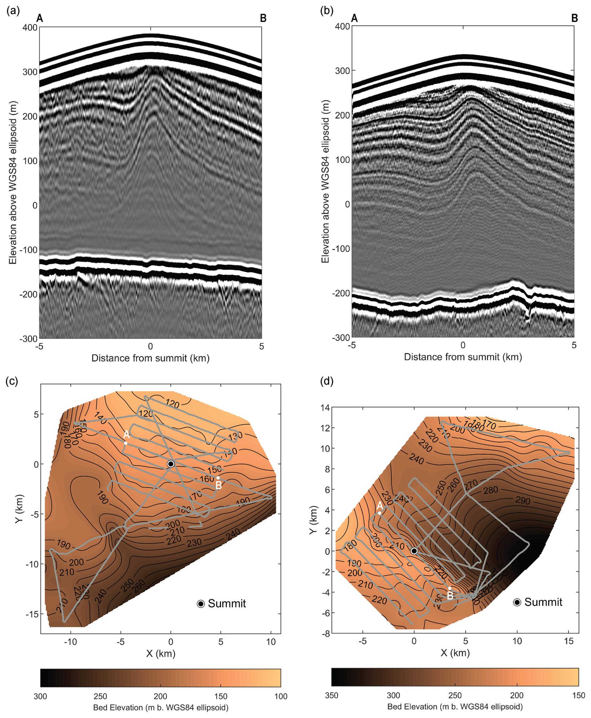
Figure 2 Deep-sounding radargrams and bed elevation maps. (a–b) 10 km-long deep-sounding radargram profiles going across the summits of KAM (Fig. 1b) and VER (Fig. 1c). The ends of these profiles (A and B) are marked in (c)–(d). (c)–(d) show the bed elevation maps for KAM and VER, respectively, with grey curves showing the location of the radar profiles used to generate these maps. The black curves show the bed elevation contours at 20 m intervals, with the labels showing the elevation below the WGS84 Ellipsoid in meters. A and B markers show the radargrams' starting and end points in (a) and (b).

3 Results: Site characteristics

3.1 Surface and bed topography

The summit of KAM is situated at an elevation of 386 m (relative to WGS84 ellipsoid) with 525 m-thick ice below (Fig. 2a). VER's summit is slightly lower at 337 m, but it rests upon a thicker layer of ice of 565 m (Fig. 2b). Both ice rises are entirely grounded below the sea level. KAM's summit lies on a gentle southward bed slope (approximately 6 m elevation gradient per km), ∼140 m beneath the WGS84 ellipsoid (or ∼155 m below sea level) (Fig. 2c). This relatively flat region spans about 4 km around the summit, with a steeper slope 7 km southeast of the summit, continuing along the ridge (north-south) and towards the survey's edge. In contrast, VER's summit is grounded deeper at around 230 m below the WGS84 ellipsoid (or ∼245 m below sea level) (Fig. 2d). The region south-southwest of the summit is rather flat (∼4 m elevation gradient per km), which transitions to a much steeper slope (∼ 18 m elevation gradient per km) just past the profile going across the summit. This slope continues farther down until the extent of our measurements.

The main difference between the bed topography under the two ice rises is that KAM has a relatively flat bed in the vicinity of the summit, whereas the summit of VER is located at the edge of a steep slope in the bed. Bilinear interpolation was used to grid the bed elevation measurements (Fig. 2c and d). While local map topography may depend on the interpolation method, the key elevation patterns are robust, as they are directly supported by the radar data.

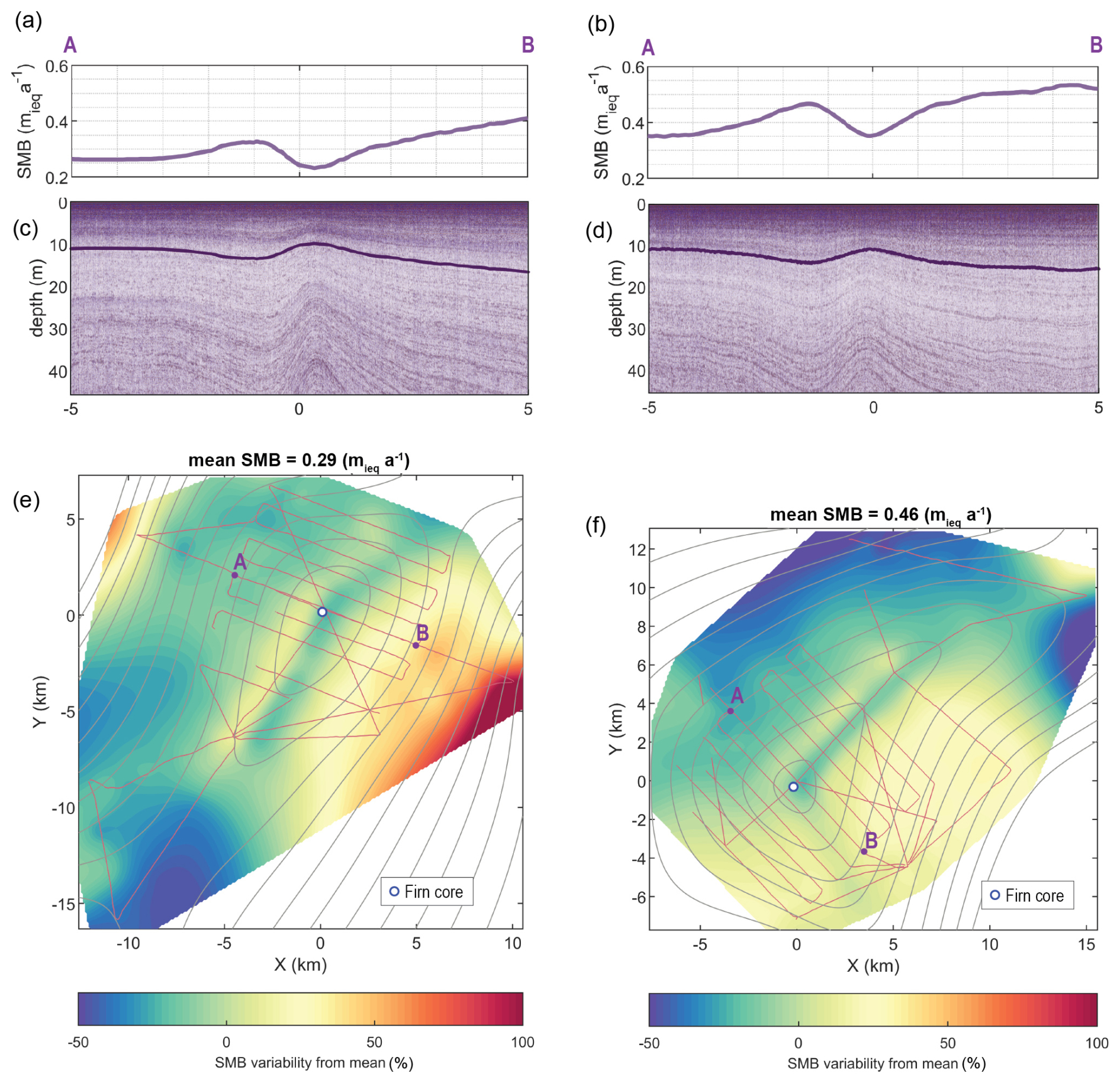
Figure 3 Shallow-sounding radargrams and SMB maps. (a)–(b) show the SMB estimated using the dated IRHs in the radargrams shown in (c)–(d). (c)–(d) show shallow-sounding radargram profiles going across the summits of KAM and VER, going from A to B. The purple curves show the tracked IRHs over the radar survey, and the white circle shows the firn core's location used to date these IRHs. (c)–(d) show the map of SMB variability (%) referenced to the spatial mean of KAM and VER, respectively, using the IRH marked in (c) and (d). A and B markers show the starting and end points of the radargrams in (c) and (d). Surface elevation contours (20 m intervals (Howat et al., 2022)) and the radar profile locations (thin red curves) are shown as references.

3.2 Surface Mass Balance

The dated shallow IRHs are used to map the spatial variability of SMB over the ice rises (Fig. 3c, d). Over KAM, the IRH dated at 30 a, demonstrates a spatially averaged SMB of 0.29 m_ieq a⁻¹. As typically observed over elevated features like ice rises, we found the signature of a strong orographic effect visible as higher SMB on the upwind eastern side (Lenaerts et al., 2014) and lower SMB on the downwind western side (Fig. 3a, e). As an example, along the profile across the KAM summit, the SMB values at 5 km on either side of the summit are 0.4 m_ieq a⁻¹. (east, upwind) and 0.25 m_ieq a⁻¹ (west, downwind). Along the ice divide, roughly perpendicular to most radar profiles, a band of low SMB is seen with a complimentary band of high SMB downwind from the ridge. This feature extends up to 8 km along the ridge from the summit, where the ridge gets less distinct and reaches a saddle. However, the absence or weakening of these bands towards and beyond the saddle could also be due to a lack of across-ridge measurements there.

VER has a higher spatially-averaged SMB of 0.46 m_ieq a⁻¹, representative of the last 22 years. The SMB distribution is similar to KAM in the sense of upwind-downwind contrast (Fig. 3b, f), with SMB values of 0.52 m_ieq a⁻¹ (east, upwind) and 0.34 m_ieq a⁻¹ (west, downwind) at 5 km distance on either side of the summit. There is a similar local band of minimum SMB along the ridge, with a complimentary band of high SMB on the downwind side.

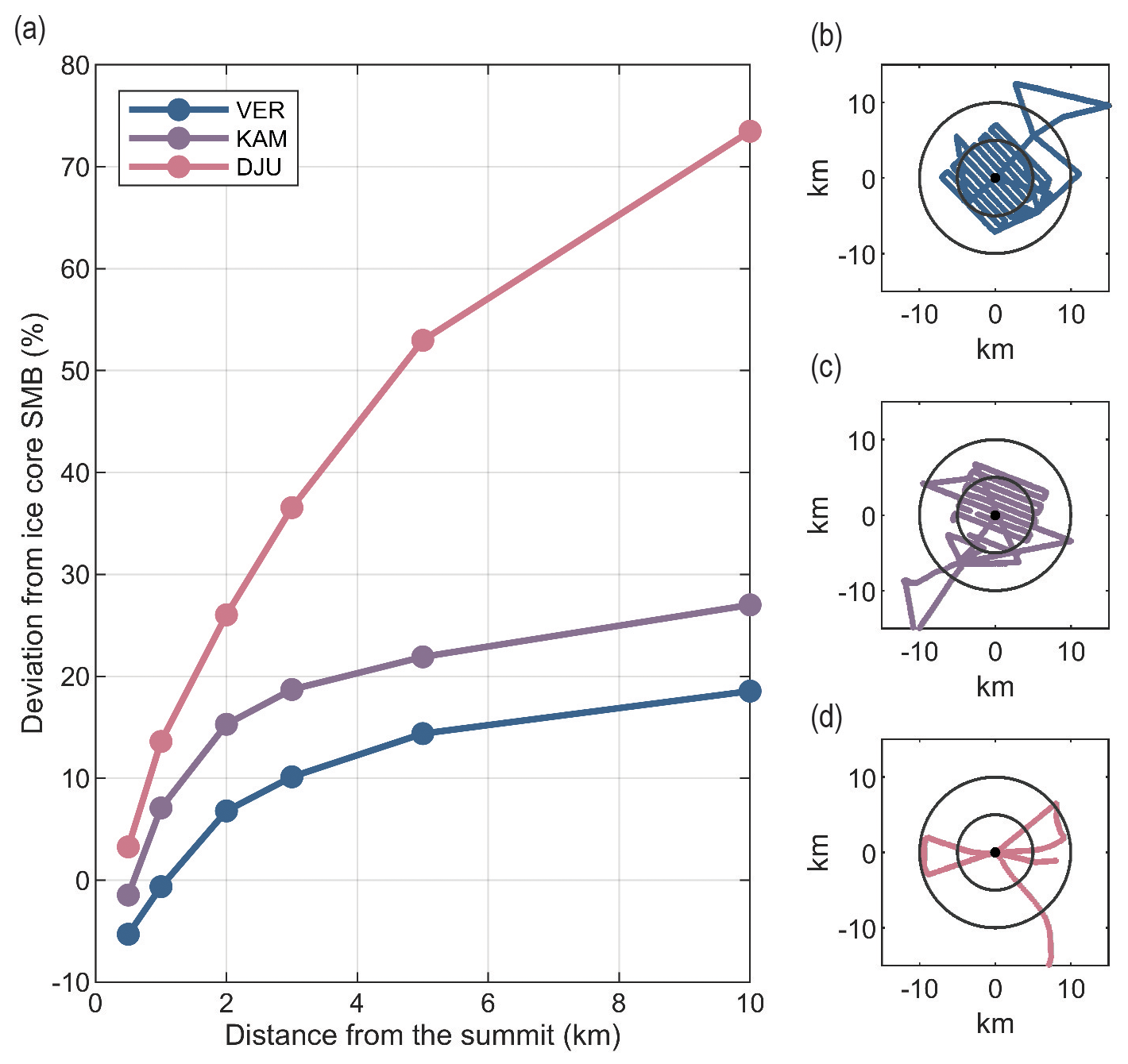
Figure 4 Spatial representativity of the ice-core derived SMB. Change in mean difference between ice-core derived SMB and mean radar-derived SMB with increasing radial data coverage from the VER, KAM and DJU ice-core sites. (b)–(d) show the coverage of the radar surveys for the three ice rises, with two concentric circles of 5 km and a 10 km radius from the summit for reference.

To assess the spatial representativeness of a potential millennia-scale SMB record from a deep ice core from these ice rises, we compared the decade-scale summit SMB from the firn cores with the spatial SMB estimates from the radar data. For this comparison, we first addressed the sampling bias inherent to the design of the radar survey by resampling the radar data onto a 50×50 m regular grid, similar to Cavitte et al. (2022, 2023). We found that as the radial distance increases, the mean difference between summit SMB and area-averaged SMB within this zone increases (Fig. 4a). This difference remains minimal within 1–2 ice thicknesses from the core site, reflecting the high variability near the summit/ice divide (Fig. 3a, e). At 5 km from the summit, VER and KAM show mean SMB deviations of ∼21 % and ∼14 %, respectively. This is lower than the earlier surveyed DJU ice rise, where a deviation of 55 % was found (Cavitte et al., 2023), indicating that ice-core-derived SMB at VER and KAM are more representative of area-averaged SMB at this distance. However, this result may have been impacted by non-even survey profile distributions at DJU (Fig. 4b, c, d). This type of fractional deviations can be considered as correction factors when comparing local ice core SMB to regional climate models which have typical grid resolutions of 5–30 km.

3.3 Englacial Stratigraphy

The deep-sounding radargrams show the englacial stratigraphy along with the ice-bed interface. On the profiles across the summits/ridges of these ice rises, we identify long-term stable englacial features known as Raymond arches (Fig. 2a, b) (Raymond, 1983). These arches are visible in all cross-ridge profiles over KAM. At VER, these arches are visible in all cross-ridge profiles and are absent in the region southwest of VER's summit, which is not characterized as divide flow.

In a theoretical steady state without any asymmetric external forcing, these arches are aligned vertically at the ice-divide position over a flat bed. However, they may be tilted or advected away depending upon the speed of divide migration relative to a characteristic timescale defined by ice thickness divided by SMB (Martín et al., 2009b). Modelling suggests that it takes one characteristic timescale for Raymond Arches to develop, and they may further evolve into a more developed double-arched shape after four characteristic timescales (e.g. Martín et al., 2009a). We used these diagnostic measures to assess the past evolution of the ice rises. The characteristic timescale for KAM is about 1800 years, and for VER, it is about 820 years; thus, VER is a more dynamic ice rise. For KAM, the Raymond Arches are vertically aligned within 1 km of the summit and do not show a double-arch shape near the bed. This suggests no significant differential changes on either flank of KAM's summit position and, thus a stable summit position for 1–4 times its characteristic time. For VER, Raymond arches under the summit are inclined away from the summit towards the east. This observed incline can be caused by a westward migrating summit position because of differential mass balance between the flanks or the effect of the locally steeping bed near VER's summit. Lastly, the possibility of uniform thinning or thickening over the ice rises cannot be ruled out based on this analysis, as it does not involve a change in the divide position.

Table 1 Characteristics of VER, KAM and DJU ice rises.

3.4 Suitability as an ice coring site

Looking at similarities, both KAM and VER are aligned along the same longitude and are of comparable geometry. Both ice rises are similarly elevated and thick around their summits with differences <60 m (Table 1). The high surface elevation of both ice rises causes relatively cold climates with minimal surface melting, as confirmed by the lack of melt features in the firn cores from their summits. However, they differ in their proximity to the sea, which could be the reason for the significant difference in their SMB, with the mean spatial SMB on VER greater than KAM by ∼50 %. The most critical differences in the context of coring site selection are bed topography and englacial stratigraphy. In contrast to the steeply sloping bed close to the VER's summit, as well as the tilt in its Raymond arches, KAM's summit is placed on a relatively smooth bed and has more vertically aligned Raymond arches. Given KAM's high suitability under site criteria (I) and (II), we tentatively conclude that KAM has a higher potential than VER as a deep ice-core site in this region. We further explore this through detailed ice-flow modelling in the following sections.

4 Results: Age modelling

Having evaluated the ice rises' glaciological settings, we now estimate the age of the ice at depth. First, we estimate the age of the ice and the expected resolution of an ice core at the summits of KAM, VER, as well as DJU for further comparison. We then focus on the most suitable site, KAM and estimate the spatial distribution of age with depth, first along a radar profile across its summit and then extending the analysis to the entire survey grid surrounding the summit. These spatial age estimates will help pinpoint an optimum drilling location on KAM.

Figure 5 Diagrams of expected age (a) and temporal resolution (b) at 20 % ice thickness above the bed in terms of ice thickness and SMB. These values at the summits of DJU, VER and KAM ice rises are also indicated. The error bars show the range of SMB within a 0.5 km radius around the summits.

4.1 Age estimates at candidate ice rise summits

Here, we estimate the age and the resolution of a hypothetical deep ice core if it was drilled at the summits of these three ice rises. For age comparison, we make the comparison at a depth of 0.2H from their beds where the expected resolution is still practicable while the ice is sufficiently old (Fig. 5a). For the 1-D model, we assume divide flow (df=1) (Sect. 2.2) and use the present-day SMB values for each ice rises summit (Table 1). We find that, while all three sites show potential for >10 ka old ice at this depth, KAM offers the potential for a significantly longer climate record at this depth. This is primarily due to thinner ice at DJU and higher SMB at VER compared to KAM.

For resolution comparison, we compare the expected temporal resolution of retrieved ice from the Last Glacial Maximum (LGM; 20 ka), regardless of the depth at which this age is reached (Fig. 5b). We find that DJU exhibits the least favourable resolution (∼5 a cm⁻¹) at 0.12H above the bed, VER an intermediate resolution (∼3.5 a cm⁻¹) at 0.12H above the bed, and KAM the most favourable resolution (∼ 2.5 a cm⁻¹) at 0.16H above the bed. As for the age-at-depth estimates, these differences are primarily caused by higher SMB at VER and thinner ice at DJU compared to KAM.

Adding to the earlier conclusion that KAM best meets the core site criteria (I) simple flow and (II) little surface melting, the modelling shows that KAM also best meets criteria (III) age and (IV) temporal resolution of a potential ice core. As all three ice rises meet criteria (V), accessibility to the core site, we conclude that KAM is the most suitable candidate to obtain long-term climate records beyond the LGM. However, VER and DJU can also be excellent ice core sites over the Holocene period due to their high SMB and associated temporal resolutions.

4.2 Spatial variability of age-depth relationship over KAM

To precisely determine an ideal site for ice coring site in the summit area of KAM, we employ the mapview method to generate spatial maps of age with depth. The primary difference in this method from the site-specific modelling (Sect. 4.1) is the use of the mapped englacial stratigraphy (i.e. tracked deep IRHs) to invert for the divide flow characteristics along the survey profiles and determine the spatial value of df. We first implement this method on a profile going across the summit of KAM and later expand the modelling scope to the complete survey grid on KAM.

Figure 6 Modelled ice ages along the summit profile of KAM. (a) Input SMB estimated used a shallow IRH dated 30 years prior (Fig. 3). (b) The tracked IRHs are shown as dark brown curves. The vertical lines show the 120 locations used for the initial age sampling step of the modelling routine, with a different colour for each location. These locations were randomly sampled outside of the divide region (<4 km from the summits). (c) The estimated df with the colours corresponding to the location of the initial sampling. (d) The isochrones modelled using the mean df (red dashed) of the 120 ensembles and the range of the isochrones modelled using the 120 ensembles df values (grey), as well as the observed IRHs (black). From top to bottom, the plotted isochrones have an age of 0.47, 0.74, 1.38, 2.20, 3.44, 4.51 and 7.23 ka. The purple vertical line shows the location of the ice divide for reference.

4.2.1 Along the profile across the summit

For the first step, we used the uppermost five tracked IRHs (Fig. 6d) as they could be confidently tracked along all survey profiles. These IRHs were dated at n random initial sampling points (n=120) outside the divide region. The 30-year averaged SMB, derived from the dated IRH along this profile, was utilized as the input SMB (see Fig. 6a). Each of these points was assigned a distinct value of p, chosen randomly from a range of 2–4. These sampling locations are depicted in Fig. 6b. For each dating instance, the optimization routine determined the values of df along the profile while minimizing for age mismatch for deep IRHs. The resulting n estimates of df along the profile are shown in Fig. 6c. Using these df values, the age-depth relationship along the profile was estimated, resulting in n different estimates. For this step, we used a fixed p value of three.

We then used these age-depth estimates to date all seven tracked IRHs. The mean age of these IRHs with their standard deviations, from top to bottom, are 0.47±0.04, 0.74±0.06, 1.38±0.15, 2.20±0.22, 3.44±0.37, 4.51±0.59 and 7.23±1.48 ka. We further compared the isochrones resulting from the mean of these estimates to the observed IRHs and found that our simple model can reproduce spatial variability in isochrone depth (Fig. 6d). The model captures the arch amplitude and the IRH slope on the eastern flank but fails to provide as good a match on the western flank or to capture the slight westward shift in the arches with depth.

Figure 7 Modelled age-depth and ice-core resolution at the summit of KAM. (a) Age and (b) resolution (a cm⁻¹) versus height above bed. Each showing ensemble mean (solid black line), median (dashed black line), and empirical probability intervals (68 % interval: 16th–84th percentiles, approximately ±1σ; 95 % interval: 2.5th–97.5th percentiles, approximately ±2σ, shaded from dark to light blue). Min/max values shown in dotted curves. The black horizontal line at 100 m above bed in (a) indicates the depth sampled for the inset histogram, which shows the distribution of age estimates at that depth with corresponding mean (red) and median (black) marked.

Age-depth estimates at the summit are shown in Fig. 7a with empirical percentile intervals: 68 % interval (16th–84th percentiles, approximately ±1σ) and 95 % interval (2.5th–97.5th percentiles, approximately ±2σ), alongside ensemble mean and median. At the summit mean and median diverge, indicating skewness in the ensemble results, as expected at the ice divide where df approaches one. Further, we calculate the depth profile of the temporal resolution of the ice core (Fig. 7b). The mean age and resolution profiles suggest an age of 20 ka at ∼80 m above the bed at a resolution of ∼ 2.5 a cm⁻¹.

Figure 8 Modelling ice age in KAM's summit vicinity. (a) Locations where the age was estimated, with magnitudes of input SMB. (b) The blue curve at the base shows the location of the available radar data. The dotted curve shows the 350 m elevation contour. The cyan colour shows the region marked as outside the divide region, with blue circles showing the location of the initial age sampling. The estimated values of parameter df are shown in (c). df was estimated at all locations shown in (a). Areas that do not show any markers in (c) have a very low (near zero) df value. (d–f) The variation of age around the summit at different heights relative to the bed. White curves are surface elevation contours at 20 m spacing.

4.2.2 Over the survey grid

Here, we evaluate the spatial distribution of age in the vicinity of the summit by implementing our method over the survey grid within 10Hd radius around the summit, where Hd stands for the ice thickness at the divide, 525 m (Table 1). For this setup, we define the divide region as the area within 4Hd from the summit and the vicinity of the southward ridge, approximated as the area where the surface elevation is higher than 350 m (Fig. 8b). As for the profile modelling (Sect. 4.2.1), we first date the IRHs at 120 random locations outside the divide area (marked with blue circles in Fig. 8b) using randomly selecting p values between 2–4. These dated IRHs were then used to invert for df over the whole region within a 10Hd radius of the summit. The inverted df values distinctly highlight the presence of divide flow with higher values along the ice rise's ridge (Fig. 8c). Using the df values and p=3, we estimate the age-depth relationship over the area within 10Hd around the summit. Estimates of the age are shown at depth-slices of 0.6Hd, 0.4Hd and 0.2Hd above the bed in Fig. 8d–f. The older ice is located along the ridge of the ice rise, with the maxima very close to the summit.

5 Limitations and uncertainties of the age estimates

5.1 Uncertainties of present-day SMB

The uncertainty in radar-derived SMB can be primarily split into three key sources: (i) the dating of the firn core, (ii) the picking of IRHs, and (iii) spatial variability in surface density. The uncertainty in the chronology of the two firn cores was calculated as the difference between the minimum and maximum age estimates at a particular depth point and was found to be ±1 year. For KAM, with an older dated IRH used for SMB estimation, the effect of this error is less significant. The uncertainty in the IRH picking method was found to be ±10 cm in ice equivalent depth. While estimating SMB, we used the same density-depth profile as measured from the summit firn cores over the whole survey. Detailed surface density measurements over ice rises along the coast of DML (46 measurements over three ice rises) show density variations of ±2.5 %–7 % around the mean values varying from 453–488 kg m⁻³ (Goel et al., 2022). With the lack of similar ground-based observations, we assume the larger ±7 % spatial variability. By aggregating these uncertainties from different sources through a root-sum-square approach, we estimated an overall uncertainty of ±8 % for the radar-derived SMB estimates.

5.2 Modelling uncertainties

For our analysis, we use a simplified 1D ice flow model and assume a steady-state mass balance scenario. We use the radar-derived SMB representative of the recent decades and assume that it represents the longer time scale of the study. The longest accumulation record closest to our sites is from the Derwael Ice Rise, further east in DML, spanning 266 years. SMB averages over 30-year intervals vary by about ±17 % (standard deviation) from the long-term mean SMB of the ice rise. Longer records from inland DML plateau (cores B31, B32, B33 from Oerter et al., 2000), spanning about 740 years, show ±6 % variability for comparable 30-year averages. An even longer 2 ka spanning SMB record exists from the Law Dome ice rise in Wilkes Land East Antarctica, which shows a variability of ±4 % for the 30-year averages (Roberts et al., 2015). Thus, to test the long-term sensitivity of our results to the single 30-year averaged radar-derived SMB for KAM, we re-run the model by scaling the input SMB by ±10 % and ±25 %. The prior cases are more plausible, while the latter is likely a more extreme case over the target 20 ka period. We find that at the summit location, for lower long-term mean SMB values (−10 % and −25 %), the 20 ka age ice is found at 71 and 60 m above the bed. For higher long-term mean SMB values (+10 % and +25 %), the 20 ka age ice is found at 85 and 100 m above the bed.

Since the survey sites have only been visited once, we do not have any field measurements of flow speed over the ice rises. Satellite-derived estimates of surface flow from image offset-tracking (Gardner et al., 2025) have too large uncertainties to capture the ice-flow pattern of these ice rises. However, field observations from comparable ice rises (Goel et al., 2022) show that the horizontal advection is small near ice divides and increases gradually towards the flanks. A simple balance velocity estimate suggests speeds of only 2.5 m a⁻¹ at a 10Hd distance from the summit. Further, we limit our analysis to within a 10Hd radius from the summit and ignore any along-ridge flow, which is likely insignificant as the slope along KAM's ridge is minimal (2.8 m gradient per km). Moreover, a direct effect of along-ridge flow would be less developed Raymond Arches (Martín et al., 2009b) than what is observed and reproduced by our model.

Bedrock topography can strongly affect the vertical ice velocity near a divide (Kingslake et al., 2014), which our 1D model does not account for. VER's bed has some strong undulations in the summit area and was thus ruled out for further consideration (Fig. 2d). For KAM, although the summit area overlies a gentle bed slope, the topography is smooth in wavelengths or amplitudes comparable with the ice thickness (Fig. 2c).

The model can reproduce the IRHs well in the divide region in the modelled profile across KAM's summit (Fig. 6d). However, on the western flank, the model cannot reproduce the observed stratigraphy well. The observed IRHs here show a syncline feature at the side of the divide. We do not observe any significant asymmetry in the bed topography across the divide that could explain the feature, with similarly smooth bed and similar surface slopes on either side. The observed mismatch on the western flank thus could be a result of a more complex 3D flow. Parrenin and Hindmarsh (2007) demonstrated that spatial variations in velocity profiles, particularly an abrupt transition from dome to flank flow regimes, can generate synclines flanking Raymond arches. A second possibility could be a gradual and systematic change in the spatial distribution of SMB with time, which is possible and has been speculated on other ice rises in the coastal DML region (Goel et al., 2018, 2022). However, both these possibilities act locally and thus should not affect our age-depth estimates near the summit.

A third possibility could be a rapid divide migration towards the east, resulting in the displacement of the Raymond Arch towards the west (Nereson and Waddington, 2002). However, the observed IRH patterns do not match those predicted by established divide migration models (Martín et al., 2009b), making this scenario less likely to explain our observations.

We implemented the ice flow in the summit area as a linear combination between flank and divide flow and used the fractional parameter df to decide the strength of the divide flow. The spatial distribution of df around the summit area (Figs. 6c and 8c) shows that on the eastern side of the divide region, df has values close to 0.5, suggesting that the flank flow itself cannot explain the IRHs in this region. Unlike the western flank, where our method fails to reproduce observations, the model matches observations well on the eastern flanks. The higher df values on the eastern flank suggest divide-flow-like characteristics in this region.

Our method aims to minimize the uncertainties related to the model. To initially date the observed IRHs, we select points outside the divide region and thus avoid the complex flow pattern near the divide, but within the region where the negligible horizontal advection assumption holds. We choose a range of likely values for parameter p, expected in this region. To assess the sensitivity of our results to the location of the initial dating and the choice of the p, we carried out Monte Carlo simulations with varying sampling locations and p values. This results in a range of df values with corresponding different age estimates. The age-depth estimates and the resulting uncertainty probability distribution (Fig. 7a) show that the uncertainty is negligible in the top half of the ice above ∼250 m from the bed. Below ∼250 m, the uncertainty increases, likely due to the Raymond effect.

6 Conclusions

This study assessed the suitability of ice rises near Maitri Station in central Dronning Maud Land (DML) for deep ice core drilling. Our field survey and detailed analysis of the ice rises Kamelryggen (KAM) and Verbljud (VER) indicate that while both sites exhibit minimal surface melting, KAM's smoother and flatter bed and simpler englacial stratigraphy make it a superior candidate for recovering a long, continuous ice core extending back to the Last Glacial Maximum. In contrast, the higher surface mass balance of VER provides excellent resolution at shallower depths for reconstructing recent Holocene climate history.

To refine the selection of an optimal drilling site within KAM, we applied a simplified map-view 1D flow model constrained by field data. We find that KAM's summit has 20 000-year-old ice preserved at about 80 m above the bed with a resolution of 2.5 yr cm⁻¹. Beyond this specific study, our modelling framework offers an efficient tool for assessing ice flow dynamics at other potential drilling sites.

An ice core record from KAM would be well-suited to investigate the nuanced interactions between sea ice, winds, and surface mass balance, thereby providing a comprehensive understanding of the regional climate dynamics in coastal DML. Ultimately, these insights will aid in refining global climate models and improving projections of future climate change in the Southern Ocean and beyond.