Reconstruction of Arctic sea ice thickness (1992–2010) based on a hybrid machine learning and data assimilation approach

Arctic sea ice thickness (SIT) remains one of the most crucial yet challenging parameters to estimate. Satellite data generally present temporal and spatial discontinuities, which constrain studies focusing on long-term evolution. Since 2011, the combined satellite product CryoSat-2 (CS2) and Soil Moisture and Ocean Salinity (SMOS), CS2SMOS, enables more accurate SIT retrievals that significantly decrease modelled SIT errors during assimilation. Can we extrapolate the benefits of data assimilation to past periods lacking accurate SIT observations? In this study, we train a machine learning (ML) algorithm to learn the systematic SIT errors between two simulations of the model TOPAZ4 over 2011–2022, one with CS2SMOS assimilation and another without any assimilation, to predict the SIT error and extrapolate the SIT prior to 2011. The ML algorithm relies on SIT coming from the two versions of TOPAZ4, various oceanographic variables, and atmospheric forcing from ERA5. Over the test period of 2011–2013, the ML method outperforms TOPAZ4 without CS2SMOS assimilation when compared to TOPAZ4 assimilating CS2SMOS. The root-mean-square error (RMSE) in Arctic-averaged SIT decreases from 0.42 to 0.28 m and the bias from −0.18 to 0.01 m. Also, despite the lack of observations available for assimilation in summer, our method still demonstrates a crucial improvement in SIT. Relative to independent mooring data in the central Arctic between 2001 and 2010, mean SIT bias reduces from −1.74 to −0.85 m when using the ML algorithm. In the Beaufort Gyre, our method approaches the performance of a basic correction algorithm. Ultimately, the ML-adjusted SIT reconstruction reveals an Arctic mean SIT of 1.61 m in 1992 compared to 1.08 m in 2022. This corresponds to a decline in total sea ice volume from 19 690 to 12 700 km³, with an associated trend of −3153 km³ per decade. These changes are accompanied by a distinct shift in SIT distribution. Our innovative approach proves its ability to correct a significant part of the primary biases of the model by combining data assimilation with machine learning. Although this new reconstructed SIT dataset has not yet been assimilated into TOPAZ4, future work could enable the correction to be further propagated to other sea ice and ocean variables.

1 Introduction

In this study, we investigate an original approach combining data assimilation and machine learning to correct past model estimations of sea ice thickness using present observations. While ground truth observations offer unparalleled accuracy, they lack global coverage, contrasting with remote sensing observations that, although global, are associated with large uncertainties due to necessary assumptions for estimation. At present, the best estimation is commonly obtained by integrating remote sensing observations into models to reduce their biases. However, this approach relies on the availability of observations and, as a result, cannot help retrieve historical sea ice thickness. Studies focusing on long-term evolution, particularly those oriented toward climate research, demand extensive and accurate time series of sea ice thickness, given the essential role that sea ice plays as the interface between the ocean and the atmosphere.

Arctic sea ice acts as a multifaceted and vital interface between the ocean and the atmosphere, playing a major role in regulating energy exchange, reflecting sunlight, and influencing local weather patterns. Sea ice significantly influences marine ecosystems, providing habitat and migration routes for diverse species (Kahru et al., 2011; Frainer et al., 2017). As sea ice melts, it injects freshwater into the ocean, affecting salinity levels and exposing the ocean to the atmosphere. Moreover, as Arctic sea ice extent is declining due to warming (Comiso et al., 2008), the Arctic is becoming more navigable, opening up new opportunities for maritime transportation and resource exploitation but also raising concerns about environmental impacts and sustainable management of the region's fragile ecosystems (Aksenov et al., 2017). Notably, the thickness of Arctic sea ice stands as a major unknown quantity, as thicker ice, usually older and deformed, resists melting and mechanical stresses better. Its variations are intricately tied to the heat and freshwater budget, the sea ice dynamics, and the ecosystem.

The current deficiency in a comprehensive and accurate climate record for sea ice thickness (SIT) is attributed to the sparse availability of SIT observations and the relatively recent integration of satellite technology. Although SIT observations have been taken in situ (Lindsay and Schweiger, 2015) and by no fewer than five satellites, they generally suffer from severe representativity issues and high uncertainties (Zygmuntowska et al., 2014) and lack both the temporal and spatial continuity that long-term climate studies need. Consequently, model reanalyses of Arctic SIT diverge substantially (Uotila et al., 2019) and lack credibility. An extended reconstruction of Arctic sea ice thickness, along with its uncertainty estimates, is essential to unlocking investigations of the Arctic climate, including heat budgets (Trenberth et al., 2019), freshwater fluxes (Solomon et al., 2021), and its ecosystem (Arrigo, 2014).

Physical-based sea ice models (e.g. Hunke and Dukowicz, 1997) can simulate reasonable sea ice thickness, yet SIT biases in numerical models remain significant, originating from various factors including external components like atmospheric or ocean fluxes and internal aspects intrinsic to the model itself. Intercomparisons of SIT between state-of-the-art models thus exhibit large deviations from one model to the next in terms of spatial distribution (Johnson et al., 2012; Uotila et al., 2019; Watts et al., 2021). Similarly, large deviations are observed when comparing satellite products (Sallila et al., 2019) or diverse in situ datasets, mostly due to differences in spatial and temporal coverage (Lindsay and Schweiger, 2015; Labe et al., 2018) and in data processing methods, such as retracking algorithms for satellite altimeters (e.g. Tilling et al., 2018; Landy et al., 2020).

Since 2010, the merged remote sensing product CS2SMOS, combining data from Soil Moisture and Ocean Salinity (SMOS) and CryoSat-2 (CS2) for thin and thick ice, respectively, provides continuous SIT every winter (Ricker et al., 2017), yet longer time series are required to conduct climate studies. Assimilating CS2SMOS data in the coupled ocean–sea ice model TOPAZ corrects a low SIT bias of roughly 16 cm, reducing average root-mean-square errors from 53 to 38 cm and further to 20 cm in March (Xie et al., 2018; Xiu et al., 2021). Can we extrapolate the benefits of data assimilation to past periods without SIT observations? Brajard et al. (2020) introduced a method to combine data assimilation (DA) with machine learning (ML) to build a hybrid numerical model. The present study applies this approach to rewind a climate record.

Machine learning has advanced to a point where it can effectively address the high dimensionality, complexity, and nonlinearity inherent in dynamical systems (Rolnick et al., 2022), especially when combined with DA (Cheng et al., 2023). Recent investigations have demonstrated the potential of machine learning for sea ice, focusing on various objectives such as parameterizing subgrid-scale dynamics (Finn et al., 2023), emulating sea ice melt ponds (Driscoll et al., 2023), or skilfully predicting DA increments of sea ice concentration across all seasons (Gregory et al., 2023). In the present study, our assumption is that a suitable compression of the variables at play (e.g. via empirical orthogonal function, EOF) identifies the complex nonlinear relationships between physical variables without altering them (Liu et al., 2023).

In the present investigation, we train a machine learning algorithm to learn the systematic SIT errors between two versions of the model TOPAZ4 over 2011–2022, with (TOPAZ4-RA) and without (TOPAZ4-FR) CS2SMOS assimilation. Then, we use the algorithm to predict the SIT error and extend the SIT estimates to periods before 2011 (Fig. 1). For this work, the training period (2014–2022) supports algorithm development and includes a validation period (20 % of the training period, in chronological order without randomization) to optimize hyperparameters. The test period (2011–2013) enables us to verify our algorithm performance using the data held specifically for this purpose. The evaluation period (1992–2010) allows us to assess the ML-adjusted SIT, called TOPAZ4-ML, compared to independent datasets.

Section 2 describes various datasets and the model TOPAZ4. Section 3 further explains the method used to combine DA and ML. Section 4 presents the results and evaluation of the ML algorithm, as well as an assessment of the extended SIT time series with independent datasets, and highlights unprecedented outcomes from this brand-new product. Section 5 discusses the limitations of and uncertainties in this investigation.

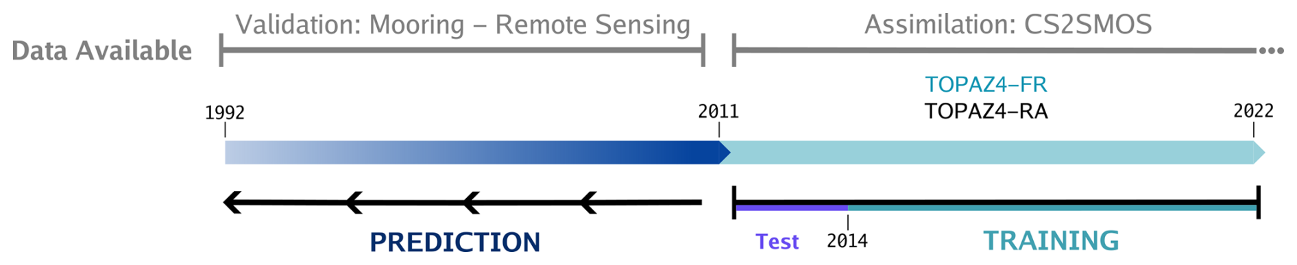
Figure 1 Chronological conception of our study. Development of the ML algorithm is based on the years 2011–2022. Prediction by the ML algorithm is done from 2011 backward in time until 1992. CS2SMOS serves as the development of our ML algorithm, while mooring data and remote sensing observations provide the evaluation of its prediction.

2 Datasets

2.1 CS2SMOS

The CS2SMOS sea ice thickness (SIT) product (Ricker et al., 2017) combines measurements from two satellite missions: CryoSat-2 (CS2) and Soil Moisture and Ocean Salinity (SMOS). CryoSat-2 (Wingham et al., 2006) utilizes radar altimetry to measure the height of the ice surface above the water level, which is converted into sea ice thickness, assuming hydrostatic equilibrium. SMOS (Kaleschke et al., 2012) measures microwave emissions at 1.4 GHz, allowing us to derive sea ice thickness from thin ice. The combination of CS2 and SMOS handles their individual deficiencies better by accurately resolving thin ($<\sim \mathrm{1}$ m) and thick ($>\sim \mathrm{1}$ m) sea ice floes, respectively. This advanced merged product provides the first accurate representation of the true sea ice thickness distribution, with temporal continuity and spatial coverage. Due to challenges differentiating between sea ice leads and surface melt ponds during the melting season, the observation period is limited to October through April, starting in 2010. The average uncertainty is typically around 0.50 m, with CS2 uncertainties ranging from 0.1 to 1 m and SMOS uncertainties less than 1.1 m in thin ice (Ricker et al., 2017). The novel year-round processing of CS2 by Landy et al. (2022) was not considered here due to artefacts in the transitions from summer to winter.

2.2 TOPAZ4

TOPAZ is a regional coupled ocean–sea ice data assimilation system successfully implemented in the Arctic Ocean operational forecast, and version 4 is described in Sakov et al. (2012) and Xie et al. (2017). It is built on the HYCOM ocean model (Bleck, 2002), coupled with a single-thickness-category sea ice model based on elastic–viscous–plastic (EVP) rheology (Hunke and Dukowicz, 1997) and rudimentary thermodynamics (Drange and Simonsen, 1996). The data assimilation is based on a deterministic formulation of the ensemble Kalman filter (DEnKF, detailed in Sakov and Oke, 2008) using 100 dynamical members to assimilate various ocean and sea ice observations (see Xie et al., 2018, 2023). Historically, the system used the atmospheric forcing fields from the European Centre for Medium-Range Weather Forecasts (ECMWF) to drive the model. To generate real-time forecasts, the system is forced by the operational weather forecast products. But for a long-time model run such as the Arctic reanalysis, we use the latest ECMWF atmosphere reanalysis product version 5 (ERA5; Hersbach et al., 2020).

Rather than learning from the winter-only satellite observations, which would not provide any information about the summer season, two model runs have been produced: without and with assimilation, covering the years 1992–2022. Both of them are forced by ERA5 and provide daily outputs on regular grids with a spatial resolution of 10 km. In this study, the raw version of TOPAZ4, without assimilation, is hereafter called the free run or TOPAZ4-FR. For TOPAZ4 with assimilation, called TOPAZ4-RA, we assimilated sea level anomalies (SLAs, https://doi.org/10.48670/moi-00146; E.U. Copernicus Marine Service Information, 2025a), sea surface temperatures (SSTs, https://doi.org/10.48670/moi-00169; E.U. Copernicus Marine Service Information, 2025b), in situ profiles of temperature and salinity (https://doi.org/10.17882/46219; Szekely et al., 2024), sea surface salinity (SSS, version 3.1 from the Barcelona Expert Center), sea ice concentrations (SICs, https://doi.org/10.48670/moi-00136; E.U. Copernicus Marine Service Information, 2025c) and sea ice drift (SID) from the Ocean and Sea Ice Satellite Application Facility (OSISAF), and we took sea ice thickness (SIT, https://doi.org/10.48670/moi-00126; E.U. Copernicus Marine Service Information, 2025d) from CS2SMOS (see Ricker et al., 2017). The assimilation is performed weekly, and SIT assimilation is only carried out from October to April after 2011. All the observations except for SSS and SID were downloaded from the Copernicus Marine Environment Monitoring Service (CMEMS). Since 2004, the ice-tethered profilers (ITPs) can provide more density-layered profiles under sea ice and provide rare information to measure polar marine environments. However, their appearance in the TOPAZ4 system within a limited representative ensemble brings considerable interference to the SIT update, especially in the summer absence of SIT observations. To overcome this nonphysical response of sea ice updating from ITPs, TOPAZ4-RA implements some specific changes that have been made based on Xie et al. (2017). In each assimilation cycle, the final optimization of the model state consists of two steps. First, all ocean variables are updated as before. In the second step, the sea ice variables are updated, but we switch off the covariance contributions from the in situ profiles. As a preprocessing step, if the sea ice concentration in the TOPAZ4 free run falls below 15 %, we interpret this as the absence of sea ice (SIC = 0 and SIT = 0) in TOPAZ4-RA. This step ensures consistent sea ice extent across the two TOPAZ4 runs, allowing the ML algorithm to concentrate solely on adjusting the SIT.

2.3 ERA5

In this study, the atmospheric fields from the latest ECMWF reanalysis, ERA5 (Hersbach et al., 2020), are used as predictors for our ML algorithm. They bring valuable information about environmental conditions that improve the bias prediction. The following variables are used at the surface level: air temperature, mean sea level pressure, total precipitation, and wind speed in the east–west and north–south directions. Daily averaged fields at a horizontal resolution of 31 km are projected onto the TOPAZ4 grid. Finally, they are processed following the methodology outlined in Sect. 3.

2.4 Sea ice age

The observed mean sea ice age (Korosov et al., 2018) is used as a predictor, which we consider more precise than a modelled one. In this product, the advection scheme predicts the subsequent creation or loss of new ice by taking into account the observed divergence or convergence, freezing, or melting of sea ice. Sea ice concentration and daily gridded drift products from the OSISAF are used by the algorithm. The primary benefit of the new technique lies in its capacity to produce unique ice age fractions for every pixel in the output result, providing the ice age's frequency distribution, which allows us to obtain the mean, median, or weighted average. This feature should aid the machine learning model, as the sea ice age is a proxy for thickness; older ice has undergone more growth, freezing, and compression processes (Liu et al., 2020).

2.5 Validation data: mooring data

In situ observations have been gathered to evaluate our ML-adjusted daily SIT at different times and places in the Arctic. Upward-looking sonar (ULS) devices are the most statistically robust instruments deployed in the Arctic to measure the sea ice draft from underneath the drifting ice pack (Krishfield and Proshutinsky, 2006). In contrast, observations from floe-tethered Lagrangian buoys only measure the thickness of the specific sea ice floe to which they are attached. The sea ice thickness from ULS can be derived assuming hydrostatic equilibrium. In this work, SIT is computed by multiplying the sea ice draft by a factor of 1.12, which corresponds approximately to the ratio of mean seawater density and sea ice density (Sumata et al., 2023; Johnson et al., 2012; Bourke and Paquette, 1989). A more precise conversion from sea ice draft to thickness is possible using the appropriate snow and ice densities (Nab et al., 2024). The datasets listed in Table 1 are used during the validation period prior to 2011. They have been collected by the Beaufort Gyre Exploration Project (BGEP; https://www2.whoi.edu/site/beaufortgyre/, last access: 5 February 2025) and the North Pole Environmental Observatory (NPEO, http://psc.apl.washington.edu/northpole/, last access: 5 February 2025). Their locations are shown in Supplement Fig. S1. We apply a 7 d running mean to smooth the mooring data, ensuring a more consistent comparison. Then we choose the nearest grid point to each mooring site and extract daily SIT values from the model at those locations.

Table 1 Mooring data used in this study. The Beaufort Gyre Exploration Project is abbreviated as BGEP and the North Pole Environmental Observatory as NPEO. ULS stands for upward-looking sonar.

2.6 Validation data: remote sensing

ICESat-1 (Ice, Cloud, and land Elevation Satellite) emerged as a pioneering instrument for the assessment of sea ice thickness, specifically in polar regions (Schutz et al., 2005). Despite its innovative approach, the Geoscience Laser Altimeter System (GLAS) encountered a malfunction that forced it to operate only for 1-month periods out of every 3 to 6 months to extend the time series of measurements. It operated from January 2003 to October 2009, resulting in 15 campaigns in the Arctic. The process of converting the retrieved freeboard and estimated snow cover climatologies is further explained in Kwok and Cunningham (2008), which allowed ICESat-1 to provide mean SIT for each campaign at a spatial resolution of 25 km × 25 km. The satellite orbital configuration causes a data gap at latitudes north of 86° N, which is filled through interpolation (Yi and Zwally, 2009).

Envisat, the European Space Agency's (ESA) satellite launched in 2002, has played a crucial role in advancing our understanding of Earth's polar regions. The dataset (Hendricks et al., 2018) provides sea ice thickness derived from the Radar Altimeter-2 instrument developed by the ESA Climate Change Initiative (CCI) project. It provides monthly gridded sea ice thickness data for the freezing period (October–March) from 2002 to 2012. The spatial resolution is 25 km × 25 km in the Arctic, with the Pole hole north of 81.5° N.

Previous studies utilizing these satellites drew the following conclusions. Envisat, with its sensor's coarse resolution (∼ 2 km footprint), primarily samples larger and thicker sea ice (Paul et al., 2018; Tilling et al., 2019), whereas ICESat-1's sensor has a much finer footprint (∼ 170 m), enabling more detailed measurements. In comparison to airborne and ULS data, ICESat-1 SIT was consistently less than that of CryoSat-2 by ∼ 50 cm (Kim et al., 2020).

3 Method of sea ice thickness adjustment

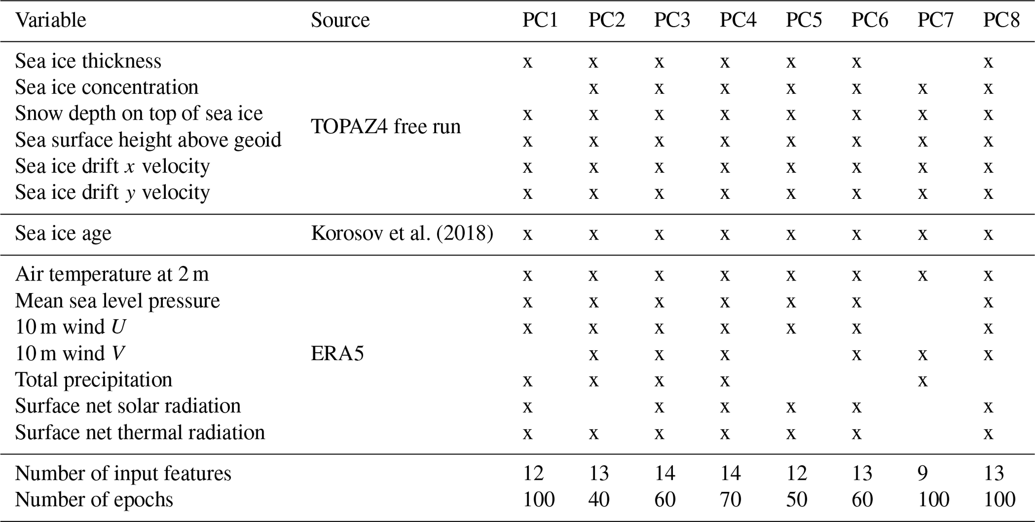
Our adjustment method is applied as a post-processing operation during the TOPAZ4 free run, dependent on the state of the sea ice but also the external forcing variables. The approach is based on the empirical orthogonal function (EOF) decomposition to reduce the dimensionality of our problem. This data compression enables us to apply a substantial adjustment that requires minimal computational resources and remains unaffected by static geographic features, such as the coastlines. During the training period (2014–2022), we compute the empirical orthogonal functions (EOFs; spatial component of the statistical patterns) and associated principal components (PCs; temporal evolution of the statistical patterns) of the SIT biases. Applying the method outside of the training period assumes that this EOF decomposition is stable back in time. Consequently, the EOFs of the SIT biases are assumed to be invariant, while the target variables to predict are the PCs of SIT biases back in time (Fig. 2). The increments from data assimilation give the best estimates of SIT biases, and we learn to emulate these increments, similarly to what is done in, for example, Brajard et al. (2020) or Gregory et al. (2023). Using the increments rather than the innovations means that the algorithm can be used with irregular observations, while the data assimilation takes care of their interpolation. Likewise, each input feature (listed in Table 2) is decomposed independently using either eight EOFs (sea ice thickness and age) or four EOFs (all other variables). At first, 14 a priori relevant features are used as inputs, and then an arbitrary threshold of the variable importance enables the adequate selection of the best-suited variables. The input features are provided to the algorithm at different time lags (in d): t−30, t−7, t0, t+7, and t+30. Considering that using eight components for the EOF decomposition of the SIT bias yields satisfactory results (Supplement Fig. S2), the subsequent results will exclusively focus on this configuration.

Korosov et al. (2018)

Table 2 List of variables used as inputs for the machine learning algorithm. An x indicates that the variable is used for the corresponding PC. The lower part of the table displays the parameters used to train each model.

Long short-term memory (LSTM) is a recurrent neural network designed to model chronological sequences and store information on a long time range (Hochreiter and Schmidhuber, 1997). LSTM estimates the current prediction using data from its own prior prediction and enables the propagation of the bias backward in time, like a nonlinear type of autoregressive process. A unique model is developed for every single PC, as each depends on different input variables and time lag. The architecture is composed of three backward-prediction LSTM layers alternating with dropout layers, which prevent overfitting by randomly deactivating neural connections during training. Hyperparameters such as the number of components of the inputs, the input variables, and their time lags can change between models, while the overall architecture remains the same. Details regarding the differences between each model can be found in Table 2. Since certain PCs proved more challenging to predict than others, a comprehensive analysis of PC prediction is provided in Appendix A to better understand the performance of each model. Throughout this investigation, we discovered that the input variables have a much greater impact on the prediction than the ML architecture.

The uncertainty associated with the nonlinear estimation is computed by introducing random-walk processes to perturb the inputs of the LSTM. Multiple perturbation instances are employed to compute the ML-adjusted SIT, and the standard deviation of the resulting ensemble of SIT predictions is used as an uncertainty estimate. It is important to note that this uncertainty solely characterizes the sensitivity of the algorithm to its inputs and does not encompass the uncertainty associated with the training process of the ML algorithm. The final uncertainty is computed using 50 members, with a random-walk perturbation of the inputs set to 100 % of the original values scaled between −1 and 1.

To predict SIT biases in the past, our method is the following. We project the values of each input variable onto its principal components. As a result, we obtain a time series of each principal component for each variable. Then, the ML algorithm predicts the PCs of the SIT bias, and thus SIT biases can be retrieved by inverting the EOF projection. Lastly, TOPAZ4-ML SIT is reconstructed by adding SIT biases to TOPAZ4-FR. For a comprehensive assessment, we evaluate the total sea ice volume as the product of the sea ice thickness with the concentration and area of each grid cell.

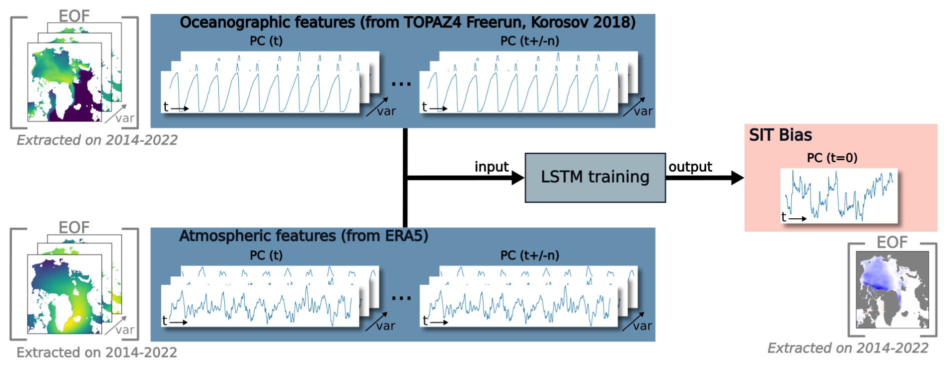
Figure 2 Illustration of LSTM prediction for one component of the EOF decomposition. The PCs of oceanographic and atmospheric features are used as inputs (blue boxes) to predict one PC of the SIT bias (red box), while the EOFs are not used as predictors (in brackets). Multiple variables (var) are used as input features at different times t and t plus or minus time lag n (because the LSTM can use input features backward or forward in time).

We introduce a trivial bias correction as a baseline to evaluate the efficiency of our ML adjustment. Monthly biases between TOPAZ4-RA and TOPAZ4-FR are averaged from 2014 to 2022. The daily baseline SIT, called TOPAZ4-BL, is then obtained by adding the monthly biases to the SIT from TOPAZ4-FR at each grid point for the corresponding month. Considering that TOPAZ4 generally has too thin SIT in areas of thick ice, even this simple baseline a priori constitutes a solid benchmark.

4 Results

After a brief analysis of the SIT biases of TOPAZ4, the sections below follow the standard steps of ML applications: first testing the algorithm on omitted data (2011–2013) and then predicting SIT biases outside of the training and testing windows, in our case extending the SIT data into the past (1992–2010).

4.1 Features of the SIT bias in TOPAZ4 between 2011 and 2022

Between 2011 and 2022, the mean Arctic sea ice thickness (SIT) within the ice edge (sea ice concentration (SIC) above 15 %) ranges between 0.6 and 2 m (Fig. 3a) for the two versions of TOPAZ4 used in this study. Both SIT simulations show a yearly cycle that is consistent with available observations. When assimilating CS2SMOS, TOPAZ4-RA SIT gets closer to the observations (Fig. 3a), and the spatial distribution improves drastically. The bias (Fig. 3b) varies from year to year and shows extreme peaks (mostly negative), often at the end of summer, as SIT errors accumulate in the absence of SIT data for assimilation. The three most recent years (2020–2022) show lower SIT biases compared to earlier years, both versus TOPAZ4-RA and in the CS2SMOS datasets. The recent decline in SIT is less pronounced in the free running model, where the ice is already thin.

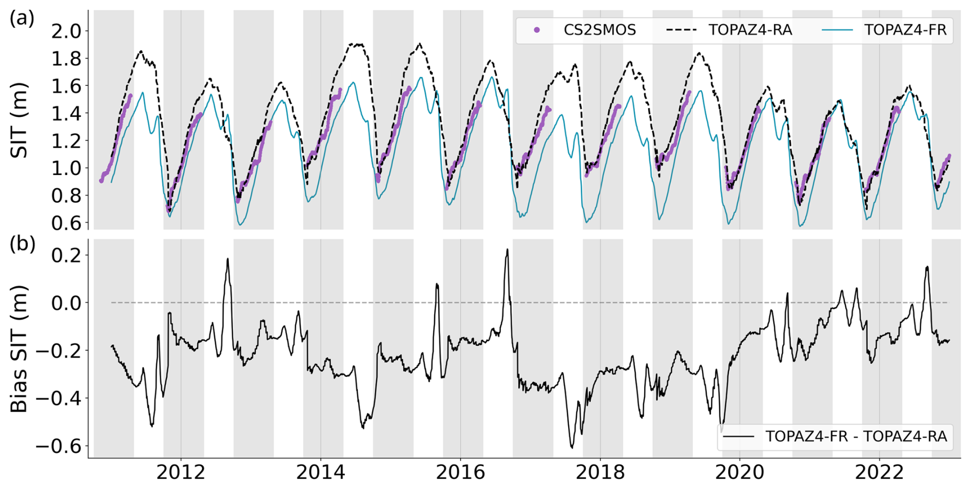
Figure 3 (a) Daily sea ice thickness (m) averaged over the Arctic within the ice edge. TOPAZ4-RA, TOPAZ4-FR, and the CS2SMOS merged-satellite products are displayed. (b) Bias of sea ice thickness (m) computed as follows: TOPAZ4-FR – TOPAZ4-RA. The freezing periods from October to April are shown with grey backgrounds.

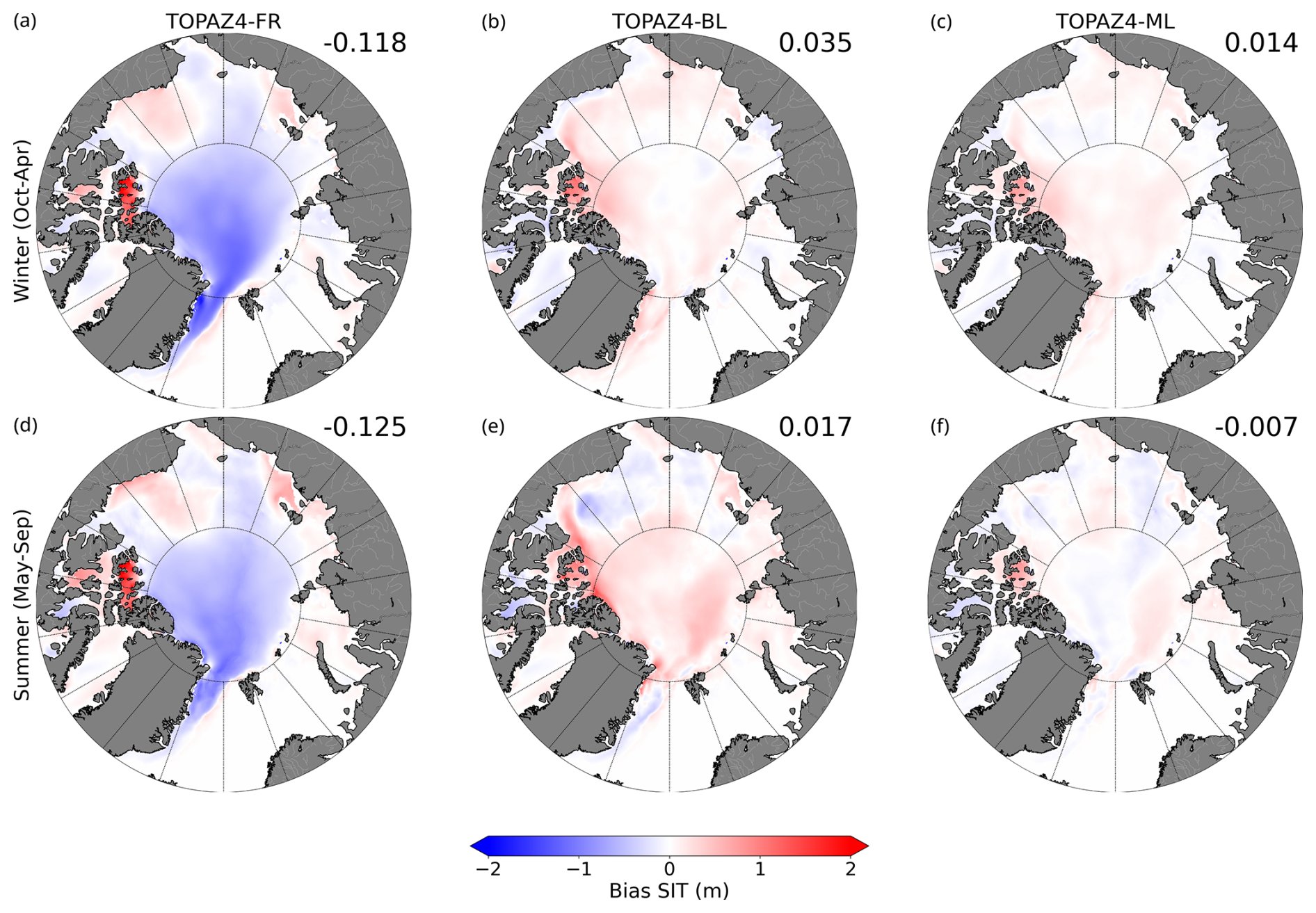
Figure 4 Seasonal bias of SIT (m) averaged over the test period (2011–2013) between (a, d) TOPAZ4-FR and TOPAZ4-RA, (b, e) TOPAZ-BL and TOPAZ4-RA, and (c, f) TOPAZ4-ML and TOPAZ4-RA. The blue colour indicates that the TOPAZ4 reanalysis SIT is thicker. The freezing period (a–c) extends from October to April, while the melting season (d–f) spans May to September.

A systematic bias in SIT can be noted all-year-round (Fig. 4). TOPAZ4-FR shows too thin ice in all areas of thick ice: the central Arctic, close to the north of Greenland, and the Fram Strait, while it depicts too thick sea ice in the Beaufort Gyre and the Canadian Archipelago. The magnitude of this error fluctuates slightly with the seasons but remains a systematic feature. The underestimation of thick ice is widespread among other models (Johnson et al., 2012; Uotila et al., 2019) and can be explained by too strong ice drift along the north of Greenland, advecting the multiyear ice westwards into the Beaufort Gyre, whereas observations show a dense and stable area of multiyear ice to the north of Greenland. The complex geography of the Arctic region, notably in the Beaufort Gyre, is prone to sea ice entrapment due to inaccurate ocean currents and winds or because of deficiencies of the sea ice rheology.

4.2 Evaluation of the ML performance between 2011 and 2013

After training the algorithm, we apply it to the period of 2011–2022 and evaluate its performance on the test dataset from 2011 to 2013, which was excluded from the calculation of the EOFs and therefore from the training. Due to the high temporal autocorrelation of SIT data over short timescales (±1 month), we chose two contiguous periods for the test and training datasets rather than using the method of random shuffling to minimize dependencies between them. From now on, the SIT predicted by our algorithm will be called TOPAZ4-ML for the sake of brevity. Our models predict the PC for each EOF (further analysed in Appendix A), which are then converted to SIT following the methodology presented in Sect. 3. Within this section, we will exclusively focus our evaluation on sea ice thickness.

As dimensionality reduction leads to an ineluctable loss of information due to truncation, the EOF decomposition introduced an inherent error into our SIT retrieval. The EOF error (Fig. 5b) represents a lower bound that even optimal ML performance cannot mitigate. The highest root-mean-square error (RMSE) values (0.5 m) are obtained in the marginal seas, particularly in the east Greenland Sea, Beaufort Gyre, and Laptev Sea regions. Conversely, the error obtained by the baseline (Fig. 5c) is considered our upper bound, being a trivial bias correction. In contrast to the lower bound, the RMSE values are much higher (up to 1.5 m) from the Fram Strait to the whole central Arctic, as well as in the Canadian Archipelago, areas where the free run is most biased. The baseline RMSEs are, however, small in the marginal seas where sea ice is thin. The ML-adjusted error reveals patterns more similar to the EOF error (Fig. 5 left). This can be interpreted as the residual error being predominantly influenced by the truncation of the EOF rather than the ML error. The ML-adjusted RMSE increases by 0.2 m compared to the EOF truncation RMSE, mostly visible in the central Arctic as well as in the Beaufort Gyre. On average, the mean RMSEs of 0.24 m (ML-adjusted), 0.21 m (EOF), and 0.31 m (baseline) attest that the ML algorithm is more accurate than the baseline, with performance close to the optimal EOF capability. Despite the large RMSE observed in the central Arctic, the baseline manages to provide an acceptable correction on average.

Similar behaviours have been noted for other error indicators, such as the bias and the correlation (not shown). This demonstrates that our methodology can reconstruct the SIT with a relatively small error induced by the ML algorithm itself and that the correction goes beyond a trivial monthly bias adjustment.

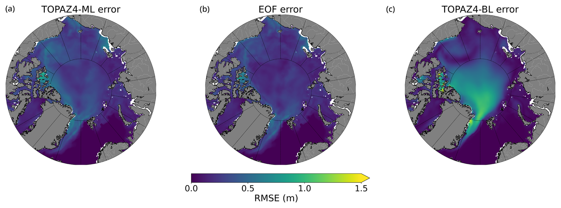
Figure 5 RMSEs of the SIT bias (m) over the test period (2011–2013) for (a) ML-adjusted error, (b) EOF error, and (c) baseline error against the SIT bias between TOPAZ4-FR and TOPAZ4-RA.

Over the test period, TOPAZ4-ML SIT is in strong concordance with TOPAZ4-RA SIT (Fig. 6), while still showing discernible differences, specifically during the melting period of 2011 and at the end of the growth period of 2013. The temporal evolution of the mean SIT for all methods, including the TOPAZ4-RA used as our reference, is shown for the entire training period in Fig. 6. These time series show the artefacts related to the experimental setup throughout the summer, mostly due to the lack of sea ice thickness assimilation. As anticipated, the ML algorithm closely aligns with TOPAZ4-RA during the training period, although the degree of agreement varies from year to year during the test period, supporting the assumption that the latter is largely independent of the training period. The baseline presents more substantial differences, mostly during the melting period as well as in the later years of thinner ice. In particular, a secondary peak of SIT that is occasionally thicker than the winter maximum stands out at the beginning of each melting period. This eye-catching feature is also observed simultaneously in TOPAZ4-FR, albeit to a lesser extent, as a statistical artefact of computing the average thickness: the thin ice melts first, and the surviving thick ice causes the average to increase where the ice is still present. It will be further addressed in Sect. 5. The baseline, however, agrees robustly with TOPAZ4-RA during the growth season. This indicates that the spatially averaged SIT bias repeats identically every year during the freezing season and could be improved by tuning a model parameter like the thickness of new ice (Wang et al., 2010) or, more preferably, by upgrading to a more advanced thermodynamical model.

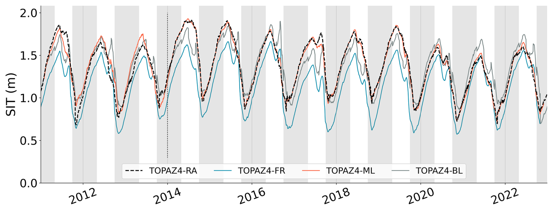
Figure 6 Daily SIT (m) averaged over the Arctic for SIC > 15 %. SITs for TOPAZ4-RA (considered our truth), TOPAZ4-FR, TOPAZ4-ML, and TOPAZ4-BL are shown. A vertical line in 2014 separates the test (2011–2013) from the training sets (2014–2022). The freezing periods from October to April are shown with a grey background.

The application of the ML algorithm results in a drastic bias reduction, outperforming the baseline. Over the test period, the mean bias between TOPAZ4-FR and TOPAZ4-RA is −10.0 cm. The year-round bias reduces to 1.4 cm after ML adjustment, with a seasonal modulation of 2.5 cm (October–April) and 0.4 cm (May–September) (Fig. 4c, f). Regarding the baseline, the averaged remaining bias is 4.9 cm, and the seasonal values are the following: 3.6 cm (October–April) and 6.2 cm (May–September) (Fig. 4b, e). Although the baseline constitutes a clear improvement during the test period, particularly during the winter season, the errors remain large in some areas (Fig. 5).

4.3 Application of the ML adjustment between 1992 and 2010

Since the ML algorithm performed well during the test period, it is further extrapolated to predict SIT biases before the CryoSat-2 and SMOS missions were launched in 2011. As suggested by Lam et al. (2023), better performance is anticipated when training on the whole dataset, so in this section, we retrained the ML algorithm, taking into account all years starting in 2011, without adjusting any parameters. Undeniably, three additional cycles of growth and melt are valuable information, especially considering that our full dataset only spans 12 years.

In the following section, we use several validation datasets (described in Sect. 2) as a series of indicators to assess the reliability of our sea ice thickness estimations. Unfortunately, the absence of a universal ground truth for sea ice thickness makes validation challenging. By presenting diverse sources of SIT, we aim to provide a comprehensive view of the legitimacy of our correction. Given the strengths and limitations of each product, we recommend that readers be mindful of differences in sea ice thickness related to various observation types, including measurement methods, processing techniques, and associated uncertainties, as well as any potential inconsistencies between products.

4.3.1 Validation with independent datasets

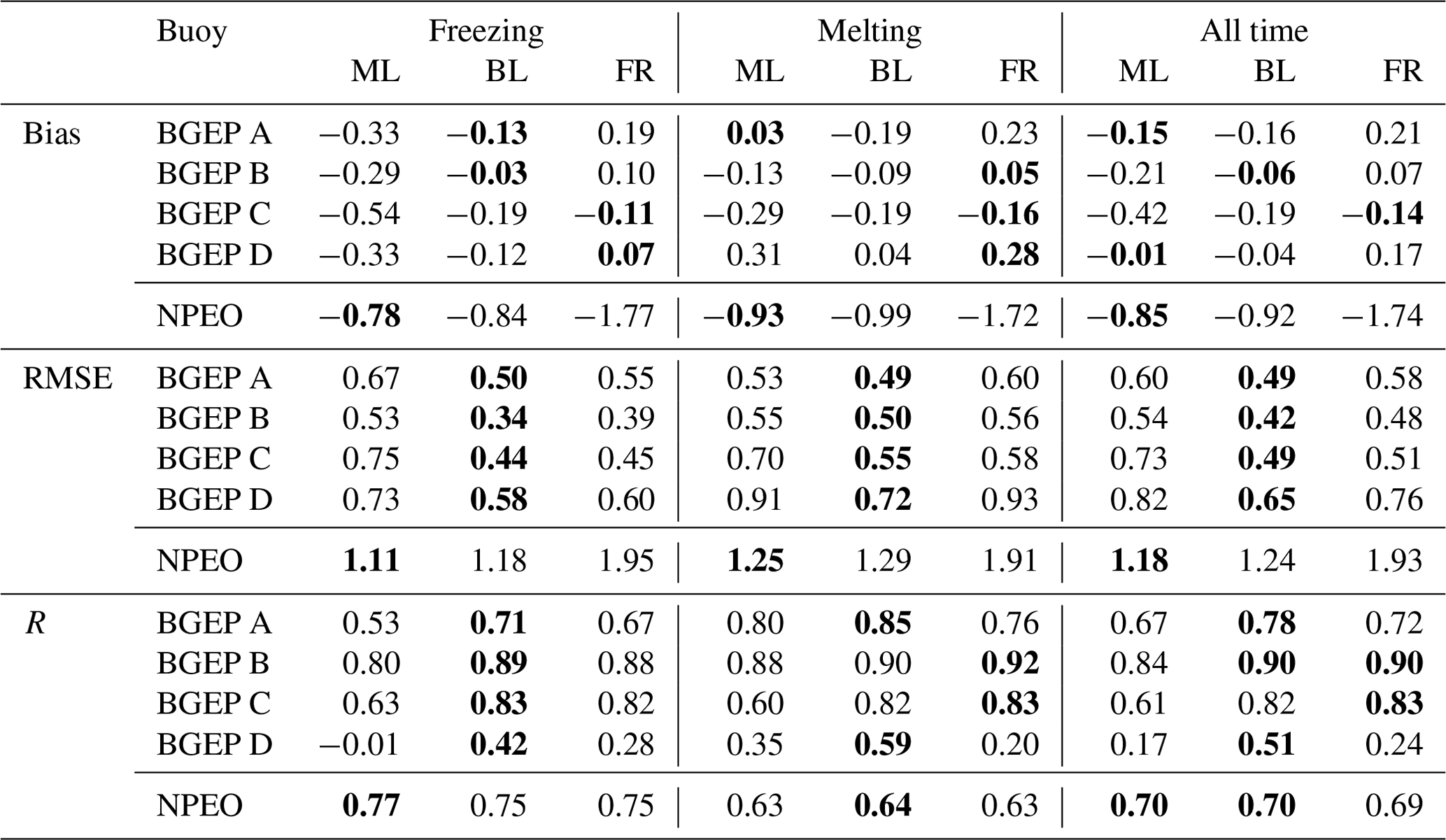
Our first step is to assess the performance of our prediction against in situ datasets during the first decade of prediction (2000–2010). In the central Arctic, TOPAZ4-ML demonstrates the closest alignment with mooring data (NPEO) compared to the baseline and the free run. In contrast, in the Beaufort Gyre, TOPAZ4-ML fails to provide the closest estimation to mooring data (BGEP), as detailed in Table 3.

We will further analyse the discrepancies by focusing on the representative case of mooring A from BGEP (Fig. 7), situated within the Beaufort Gyre. While it shows a clear enhancement over the melting season when contrasting TOPAZ4-FR and TOPAZ4-ML SIT, the freezing season reveals less consistent agreement, indicating weaker performance. Overall on buoy BGEP A, TOPAZ4-BL exhibits the best performance based on all statistical indicators, followed by TOPAZ4-ML and then TOPAZ4-FR. The baseline always underestimates SIT at the onset of the melting season, an issue that is potentially specific to the Beaufort Gyre region, as it is the only area where the free run systematically overestimates SIT. The SIT data from the buoy exhibit considerable variability, particularly towards the end of 2006 and during the transition between 2007 and 2008. This variability might be attributed to the specific climatic conditions during those years, notably 2007, which marked a record-setting ice retreat characterized by the flushing of old and thick sea ice, and we do not expect a coarse resolution model like TOPAZ4 to render this level of variability.

The mooring is occasionally in open water, while the free run still has ice covering it. Since both the baseline and the ML algorithms are not trained to reduce ice edge discrepancies, their performance is poor during these periods. On the positive side, the time series does not indicate that the adjustment methods degrade further back in time, so the extrapolation yields reasonable values.

The improvement in the ML compared to the baseline is less striking than during the test period, mostly because assessing one specific location over a brief time period may not provide sufficient representativity to distinguish between these two adjustment methods. Additionally, the Beaufort Gyre displays different error patterns compared to the central Arctic, which might explain why the ML algorithm reduces bias more efficiently in the central region than in the Beaufort Gyre when compared to buoys. While exploring various ML configurations (e.g. different input features and numbers of epochs), an earlier experiment determined that TOPAZ4-ML achieved the closest agreement with mooring data compared to TOPAZ4-BL and TOPAZ4-FR in the Beaufort Gyre across all seasons. Ultimately, we selected the current ML configuration, which displayed the best performance during the test period without relying on past observations for calibration. Future versions of this dataset could consider incorporating similar calibration techniques to potentially improve results.

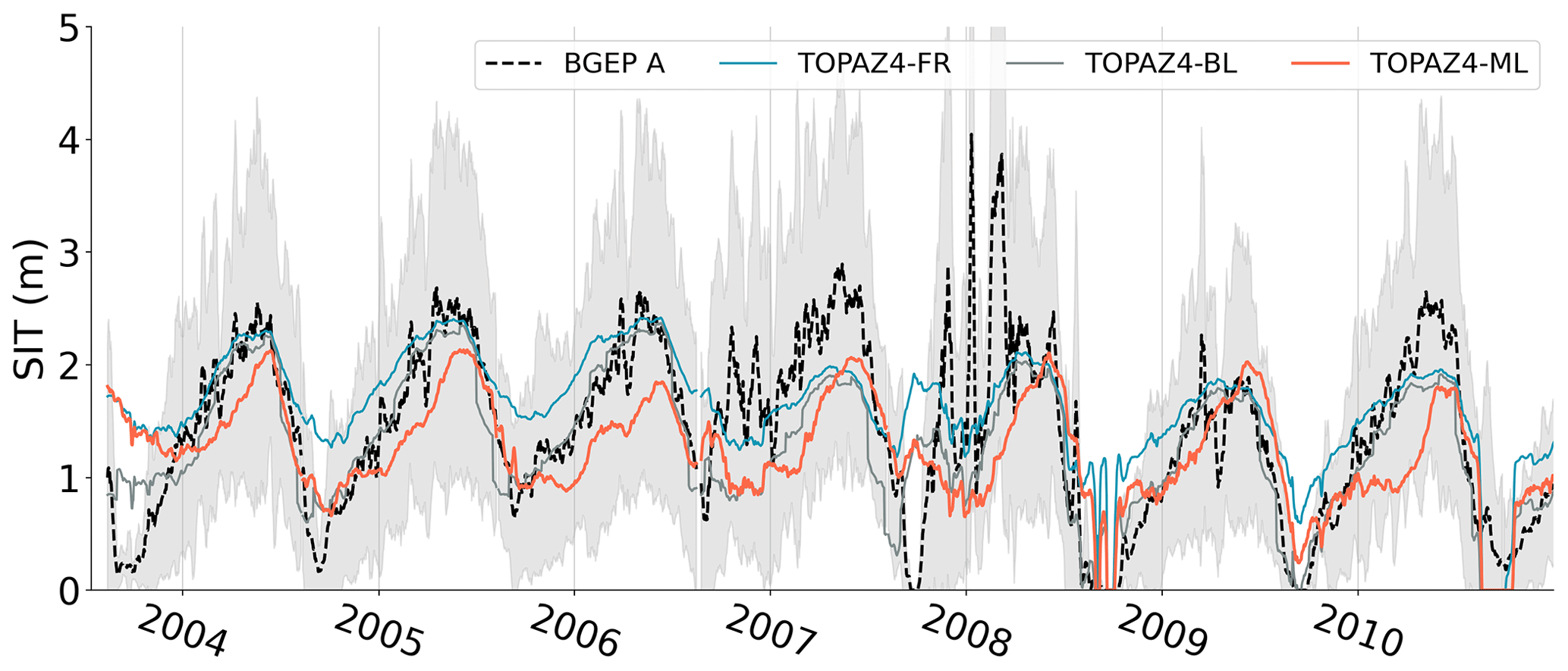
Figure 7 Daily SIT (m) for the buoy BGEP A, the TOPAZ free run, the baseline, and ML-adjusted SIT. The standard deviation of SIT for ULS BGEP A is displayed in grey.

A qualitative comparison between remote sensing data and TOPAZ4-ML (Fig. 8) exhibits close agreement in SIT and spatial distribution patterns, indicating that our reconstruction effectively behaves as a coherent correction when applied to the past. To compare these products, monthly values averaged over October between 2003 and 2007 are considered for TOPAZ4, Envisat, and the Pan-Arctic Ice–Ocean Modeling and Assimilation System (PIOMAS; Schweiger et al., 2011, described in Sect. 4.3.2), while ICESat-1 campaigns do not precisely align with calendar months. TOPAZ4-ML enhances the SIT gradient from Greenland to the North Pole, addressing the well-known issue of a flattened gradient of sea ice thickness as one moves away from the northern coast of Greenland, which can be seen in TOPAZ4-BL/FR and PIOMAS. TOPAZ4-ML and remote sensing show similar patterns within the Beaufort Gyre and Canadian Archipelago, whereas TOPAZ4-BL displays a comparable correction but with insufficient intensity. Considering Envisat SIT, we observe significantly less young and thin sea ice around the periphery of the central Arctic when compared to other datasets. As a consequence, Envisat shows high SIT (>2 m) in March (Supplement Fig. S3) near the sea ice edge in the Barents Sea, a scenario considered unrealistic and that is consistent with past reports of Envisat's tendency to overestimate SIT compared to other datasets (Paul et al., 2018; Tilling et al., 2019). Additionally, while PIOMAS SIT appears to be lower than that of ICESat-1 and Envisat along the coasts of Siberia and Alaska, it is generally consistent with satellite observations in the central Arctic along 80° N.

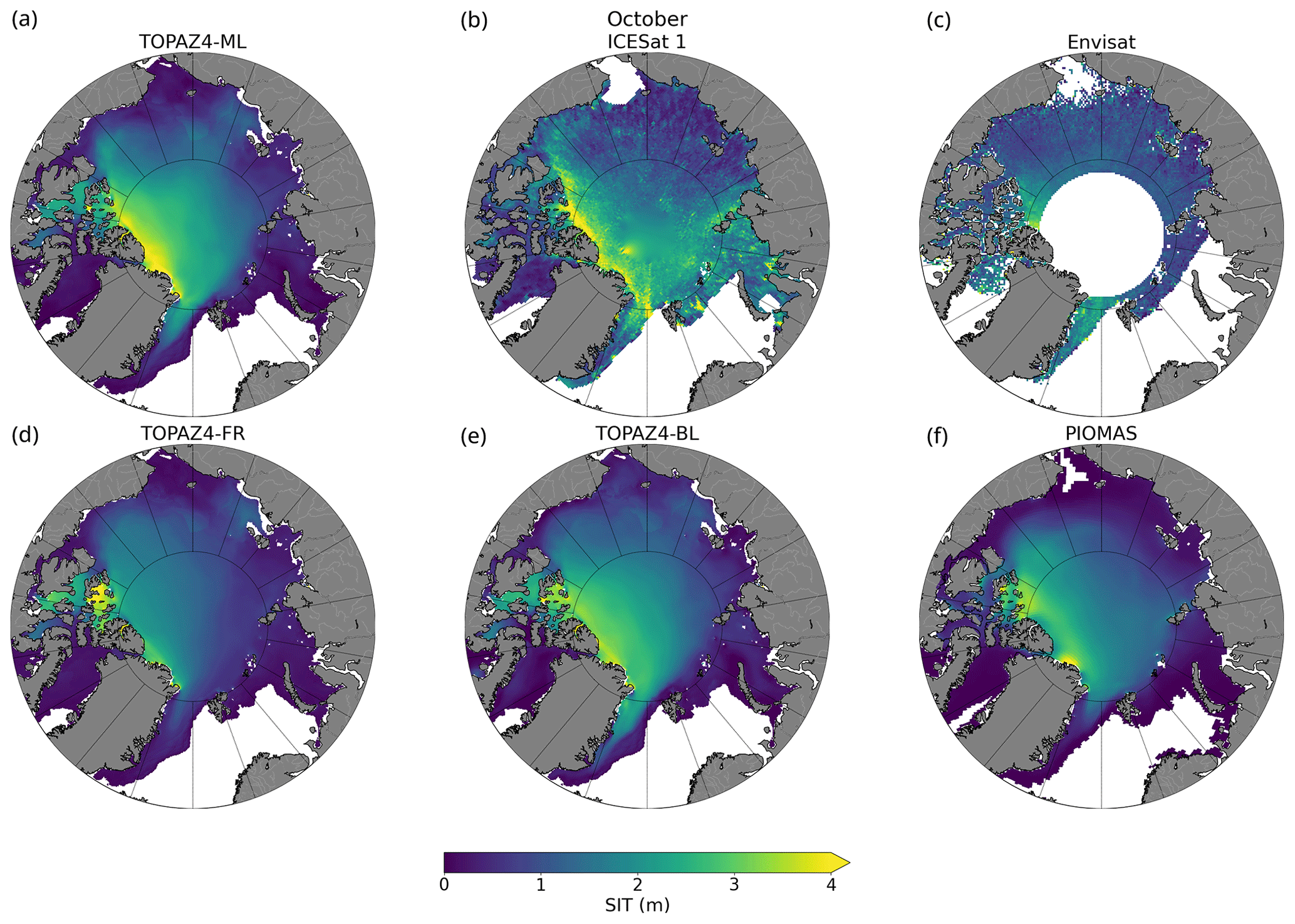
Figure 8 Sea ice thickness (m) for (a) TOPAZ4-ML, (b) ICESat-1, (c) Envisat, (d) TOPAZ4-FR, (e) TOPAZ4-BL, and (f) PIOMAS averaged over Octobers between 2003 and 2007. The ICESat-1 observation period varies, extending into November depending on the year.

Table 3 Sea ice thickness bias in metres, RMSE, and the Pearson correlation coefficient (R) between SIT from TOPAZ4-ML (ML), TOPAZ4-BL (BL), and TOPAZ4-FR (FR) and in situ datasets. The highest score is highlighted in bold.

4.3.2 Comparison with other datasets

This section compares SIT time series from 1992 to 2022 with three pertinent datasets: one widespread model reconstruction (PIOMAS; Schweiger et al., 2011) and two satellite datasets using altimeters (Bocquet et al., 2023) and passive microwaves (Soriot et al., 2024b), which are two completely different remote sensing principles. PIOMAS (the Pan-Arctic Ice–Ocean Modeling and Assimilation System) is a coupled sea ice–ocean model that assimilates several observations to improve SIT, including SIC from passive microwave satellites and sea surface temperature and sea ice velocity. Bocquet et al. (2023) provide SIT estimations from the European Remote-Sensing Satellite (ESR-1), ESR-2, Envisat, and CryoSat-2 and ensure consistency over all altimeters using a neural-network-based method. Soriot et al. (2024b) estimate SIT using a neural network based on 18 and 36 GHz brightness temperatures, measured by the Special Sensor Microwave/Imager (SSM/I) and the Special Sensor Microwave Imager Sounder (SSMIS) sensors. The two satellite products have different Polar holes, so all data above 81.5° N have been removed for consistent coverage, meaning that the results described in this section mostly apply to first-year ice. This section does not intend to identify the most accurate SIT or to explain the differences between datasets. Rather, our objective is to provide a clear comparison of how our TOPAZ4-ML SIT performs relative to other relevant datasets.

March and October trends (Fig. 9) are considered proxies for the evolution of the seasonal maxima and minima of sea ice thickness averaged over the Arctic. March was used, as it is the latest month available before the melting season in Soriot et al. (2024b).

Decreasing trends align relatively well across datasets in March (−0.21, −0.13, −0.10, and −0.19 m per decade for TOPAZ4-ML, PIOMAS, Bocquet23, and Soriot24, respectively), while October trends show more pronounced discrepancies (−0.22, −0.26, −0.11, and −0.36 m per decade). In October, Soriot24 has the strongest trend (−0.36 m per decade) compared to model-based SIT (TOPAZ4-ML and PIOMAS), while the trend in Bocquet23 is the weakest (−0.11 m per decade).

This distinctly different behaviour of model-based (TOPAZ4-ML and PIOMAS) and observation-based SIT (Bocquet23 and Soriot24) also appears in the mean values. For instance, Bocquet23's mean October SIT values are remarkably high after 2014 compared to other datasets (around 1.2 m, while others are between 30 and 90 cm). Furthermore, the October SIT mean is consistently lower for model-based estimates throughout the entire time series. In October, SIT values exhibit greater interannual variability within individual datasets compared to March, and the differences between datasets are also more pronounced.

This intercomparison shows that all datasets demonstrate realistic SIT values. This section highlights the differences in SIT among datasets and emphasizes the importance of having diverse products derived from varying primary data sources and methodologies, given the absence of ground truth.

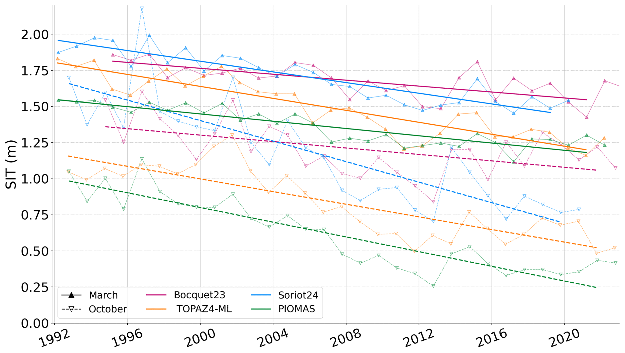
Figure 9 Monthly mean sea ice thickness over the Arctic (latitudes < 81.5° N) for March and October from 1992 to 2022. The datasets displayed include TOPAZ4-ML (this study), PIOMAS, Bocquet et al. (2023), and Soriot et al. (2024b). Trends are shown for the entire time period.

4.3.3 Interpretation of the reconstructed data

The first section validated the reconstructed SIT, while the second positioned it within the context of other relevant products. Here, we will evaluate the consistency of TOPAZ4-ML SIT over the whole Arctic, for which there are no observations available. This section will quantify various trends and changes identified with this new dataset over time.

The May (October) mean sea ice thickness in 1992 is estimated at 2.16 m (1.08 m), while in 2022, it shrunk down to 1.54 m (0.57 m). In total volume, this corresponds to 26 605 km³ (12 575 km³) and 18 804 km³ (6258 km³), with linear trends of −3274 km³ per decade (−3002 km³ per decade). The year-round trend is −3153 km³ per decade according to our reconstruction, while the PIOMAS model reconstruction estimates a slightly steeper trend of −3583 km³ per decade.

We observe a significant downward trend in the mean SIT from 2002 to 2012, surrounded by two periods without distinct trends (Fig. 10b). Our ML-adjusted SIT respects this behaviour qualitatively and does not introduce unrealistic trends by extrapolation.

Sumata et al. (2023) show how the distribution of SIT exiting the Arctic through the Fram Strait changed throughout the past 2 decades, as observed by moored upward-looking sonar devices. They reveal a bimodal distribution and a regime shift following the sea ice minimum of summer 2007. Since the Transpolar Drift brings sea ice from large stretches of the Arctic into the Fram Strait, the representativeness of these moorings is higher than in most other locations. Some delay should, however, be expected due to the advection time to the Fram Strait, which can take anywhere from months to a couple of years depending on the origin of the ice.

The yearly cycles of the main modes of SIT look generally continuous in TOPAZ4-ML (see Fig. 10a), except for a few occasional discontinuities. So the combination of DA and ML did not seem to cause much distortion of the physical signals. The TOPAZ4-ML SIT distribution of the whole Arctic also exhibits a more gradual transition from a bimodal distribution (before 2007) during the growth period to an unimodal distribution (after 2007), as depicted in Fig. 10a Prior to the 2007 minimum, a significant portion of the ice was thicker than 2 m. However, after 2008, only thinner sea ice was observable year-round. At the end of the melting period in the years before 2007, when most of the first-year ice had melted, the median sea ice thickness fell within the 1 to 2 m range. In contrast, after 2007, the median sea ice thickness has been almost consistently below 1 m. Moreover, the distribution of the thickest sea ice (depicted in green in Fig. 10a) is notably diminished when comparing the periods before 2007 (4–5 m) and after 2007 (3–4 m). The area-average SIT (Fig. 10b) is broadly similar between TOPAZ4-RA and TOPAZ4-ML, all lying consistently about 20 cm above TOPAZ4-FR throughout the whole time series. Compared to TOPAZ4-ML, PIOMAS indicates an earlier onset of the melting period, while exhibiting a similar average of SIT throughout the time series, except for the period after 2020 (Supplement Fig. S4). Contrary to the sea ice extent time series, the record minima of SIT are somewhat less spectacular, indicating that significant ridging may occur during years of the lowest ice cover (Regan et al., 2023), piling up sea ice vertically rather than horizontally. The years 2011 and 2012 are clear minima of the SIT in all datasets, in agreement with the PIOMAS model. The disagreements between the free run and other datasets are more important in the later years, as the free run indicates minimum years between 2017 and 2021, while the TOPAZ4-RA and TOPAZ4-ML datasets instead point to 2021 and 2022 as minimum SIT years. Surprisingly, summer 2007 does not stick out in the area-averaged SIT time series, as the regime shift seems to spread over a few years. In the Discussion section, we will compare various trends reported in the literature.

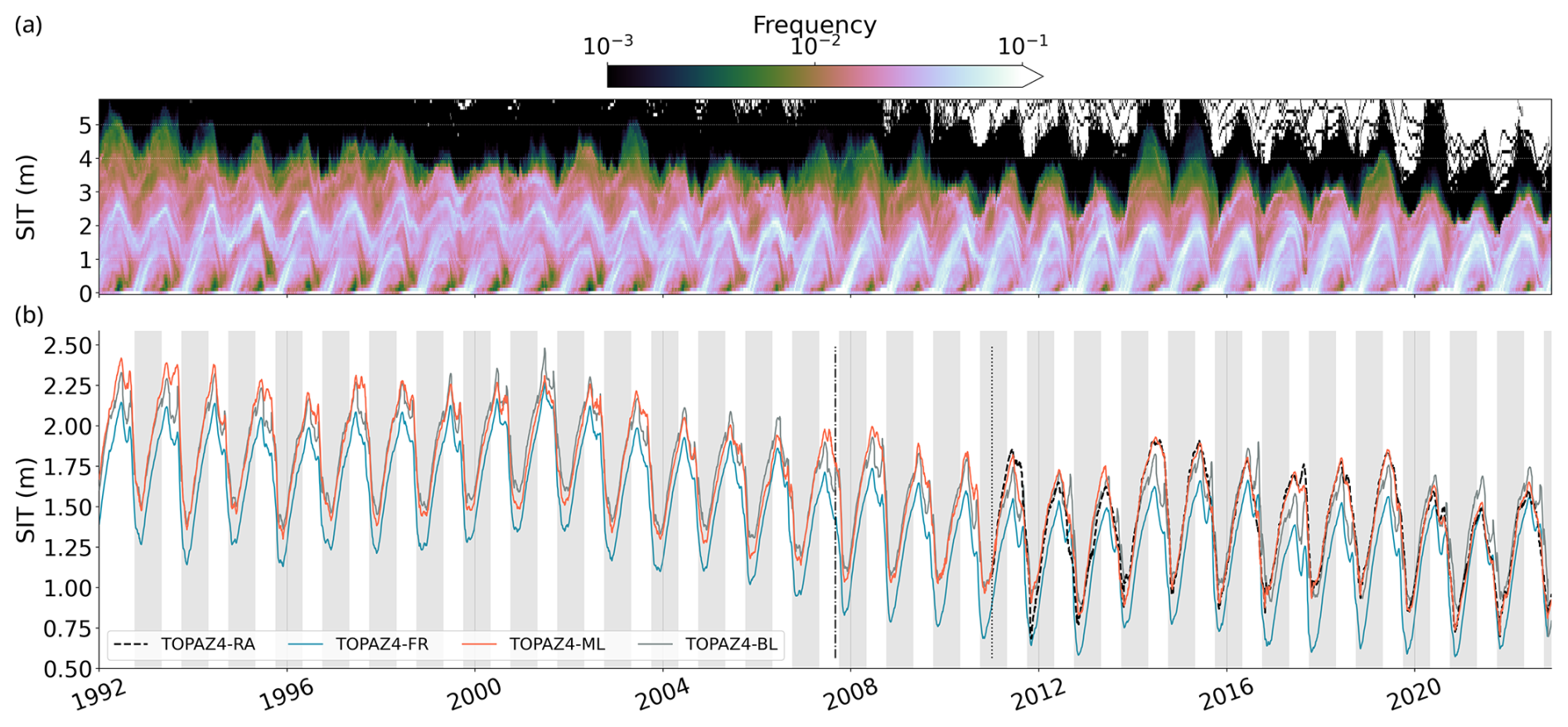
Figure 10 (a) Distribution of daily TOPAZ4-ML SIT (m) from 1992 to 2022. Bins of 0.1 m are used, and the colour bar is a log scale. (b) Daily SIT (m) averaged over the Arctic for SIC > 15 % for the same period. The ML algorithm has been retrained with 2011–2013 included, as indicated by the vertical line in 2011. The dot-dashed vertical black line marks September 2007. The freezing periods from October to April are shown with a grey background.

5 Discussion

The novelty of the present study lies in the combination of ML and DA to adjust sea ice thickness backward in time over a long period, longer than the training period. Since 1990, the sea ice thickness distribution in the Arctic has shifted drastically towards thinner sea ice (Sumata et al., 2023; Lindsay and Schweiger, 2015), as documented by both satellite and in situ data. With our adjusted dataset (TOPAZ4-ML), the mean sea ice thickness in May (October) 1992 is 2.16 m (1.08 m), while in 2022, it is 1.54 m (0.57 m), resulting in a decrease of 29 % (47 %). Using independent data in the Arctic Basin, Lindsay and Schweiger (2015) found that the annual mean SIT over the period of 2000–2012 declined from 2.12 to 1.41 m (34 %), while September thickness declined from 1.41 to 0.71 m (50 %). When including all the marginal seas up to the 15 % isoline of concentration, we find that the annual SIT is generally lower, but the trends are compatible, reducing from 1.51 m in 2000 to 1.01 m in 2012 (33 %), while September thickness declined from 1.42 m to 0.81 m (43 %). In our estimation, the annual mean sea ice thickness is lower compared to Lindsay and Schweiger (2015) due primarily to differences in the area considered. These disparities diminish in September as the residual sea ice shrinks toward the central Arctic. Kwok (2018) reported losses of 2870 km³ per decade in winter (February–March) for 15 years of satellite records (2004–2018) from the non-overlapping ICESat and CryoSat-2 periods. For the same period, the TOPAZ4-ML data indicate losses of 2941 km³ per decade (Fig. B1), which falls well within the uncertainties caused by the lack of snow depth data (Zygmuntowska et al., 2014). PIOMAS, another data assimilation model, shows trends of −2.7 and 3.2 ± 1 × 10³ km³ per decade for April and September, respectively, from 1979 to 2018 (Johannessen et al., 2020, Fig. 5.24). In comparison, over the period of 1992–2022, PIOMAS indicates −3.0 and −3.8 ± 1 × 10³ km³ per decade, while TOPAZ4-ML shows trends of −3120 and −2960 km³ per decade for April and September, respectively. Although the two datasets align well for April, a notable discrepancy emerges in September, with PIOMAS indicating a more pronounced downward trend. Drawing from the range of available data, the ML-adjusted trends correspond closely to those documented in the existing literature. Although TOPAZ4-FR and TOPAZ4-ML differ significantly in the total SIT, their respective trends are close.

By training our algorithm over the latest decade to predict the past, we assumed the following: the EOFs obtained from the SIT bias between 2011 and 2022 are representative of the statistical behaviour of the errors made by the model over a longer time period, including a dramatic regime shift. To probe the robustness of this assumption, we extracted the EOFs over two subperiods of our dataset: the training period with and without the test period. We only found differences in the least important components (from the sixth and further), while showing similar patterns overall (Supplement Fig. S5). The time series of the differences only shows unstructured noise.

Moreover, since we lack summer SIT observations, we assess the differences in SIT between two versions of TOPAZ (with and without assimilation) and not the SIT directly, so the data assimilation residuals may also have caused some loss of signal for the ML. However, the ML algorithm can adjust the thickness even of the thickest sea ice (>6 m) with less than 20 % error (Fig. C1), which explains its performance in an earlier period dominated by multiyear ice.

Our approach based on EOF decomposition enables a drastic reduction in dimensions, leading to fewer parameters in the ML algorithm and thus reducing the costs required to train and apply the algorithm. This method is fast to implement and execute (around 1 h on a personal laptop), requiring minimal computational resources. Given its effectiveness, it demonstrates a strong ability to correct a large number of the biases. In comparison, approaches relying on more intricate 2D neural-network layers produced comparable outcomes but at a higher cost (at least 12 h to train) and in a more complex setup. Additionally, it is possible that with higher-dimensional features, the training set would be too small, increasing the risk of overfitting.

Multiple ML models (LSTM, convolutional neural network, dense, extreme gradient boosting, and random forest) were tested, yielding small local variations but no visible advantages in overall performance between models. The decision to select LSTM was thus driven by its robust time series prediction capabilities and its slightly better results. Throughout this study, the ML architecture (i.e. number of layers and hyperparameters) only played a minor role in achieving the optimal prediction; instead, the prediction accuracy is considerably dependent on the input variables, i.e. the choice of variables and associated time lags.

Three distinct sources of errors were identified when predicting SIT before 2011: ML reconstruction error, errors in the free run of TOPAZ4, and errors induced by regime shifts in sea ice conditions. Since the latter two are impossible to obtain within the scope of this study, we can only provide uncertainty estimates related to the ML method itself. Note that the uncertainty obtained here only characterizes the sensitivity of the algorithm to its inputs (details in Sect. 3). The areas exhibiting the highest uncertainty encompass the Fram Strait; the Canadian Archipelago; the Beaufort Gyre; and, with a lower degree of uncertainty, the East Siberian Sea (Supplement Fig. S6). Upon examining the temporal evolution of uncertainty (Supplement Fig. S7), it appears that uncertainty diminishes during both the growth and melt phases of sea ice, likely attributable to the strong sea ice thickness seasonal cycle. Moreover, higher uncertainty is noted during the peak of the winter and summer seasons, when sea ice thickness is less affected by predominant freezing or melting, potentially leading to divergence among individual members.

Despite the baseline yielding good average results, the trivial bias correction displays strong regional biases and mediocre performance during outlier years. In addition, we expect the performance of the baseline to decrease even further as we extrapolate back in time. Indeed, the correction of the baseline is applied once and relies solely on the patterns of mean bias observed during 2014–2022, with no ability to accommodate different environmental conditions. On the contrary, our ML adjustment method proves more adaptable when predicting back in time since it takes into account the past state of environmental variables and the varying relative importance of each component (as independent errors identified by the EOF decomposition).

A distinct feature appears in the SIT averaged (Fig. 3) at the onset of the melting season: a second peak, brief compared to the first, occurs shortly after the SIT maximum. It is observed almost yearly in TOPAZ4-FR but only twice (2017 and 2020) in TOPAZ4-RA. The phenomenon can be explained as follows: the relatively thin sea ice melts first, decreasing the area faster than the thickness, thus increasing the average SIT as a case of survivorship bias. This survivorship bias may intensify in cases of erroneously thinner sea ice in the central Arctic. Such instances can arise from either thinner sea ice in the central Arctic (TOPAZ4-BL) or misplaced thick sea ice in the Beaufort Gyre (TOPAZ4-FR). To prevent this artefact, many studies prefer to use the total volume or a geographic restriction to an area of perennial ice in the central Arctic.

Comparing TOPAZ4 to in situ datasets is challenging, primarily due to representation errors. Knowing the true sea ice thickness remains a major issue for evaluation, particularly when considering historical data from older satellite missions such as ICESat-1 and Envisat. This issue becomes more pronounced as we delve further into the past. Large uncertainties linked to in situ observations and the model ultimately lead to differences in SIT and difficulties evaluating our product. Adding to this point, the limited availability of global datasets over extended periods in the Arctic restricts the scope of possible comparisons. One notable advantage of our methodology is its capacity to bridge data gaps when mooring observations are unavailable.

6 Conclusions

In this investigation, we demonstrated that machine learning (ML) can be combined with data assimilation (DA) to predict sea ice thickness (SIT) errors backwards in time to 1992, using the ice–ocean model TOPAZ4 and atmospheric variables from the ERA5 reanalysis. The SIT biases are the results of accumulated increments from the assimilation of sea ice thickness data from CS2SMOS every 7 d between 2011 and 2022 during the ice growth period (October–May). Then, we reduced the dimensionality of the DA increments using empirical orthogonal functions (EOFs). The LSTM learned to predict SIT biases using principal components (PCs) of various sea ice, ocean, and atmospheric variables as inputs. This study demonstrates that our PC-based approach is effective at providing a major sea ice thickness adjustment.

Our approach significantly reduced sea ice thickness biases throughout the test period (2011–2013) from a low year-round bias of −10.0 to 1.4 cm. Significant improvements are noted during the melting period, likely attributable to substantial errors in TOPAZ4 with assimilation, as sea ice thickness data assimilation is unavailable during summer. Applying our algorithm before 2011, the evaluation with independent mooring data indicates improvement in the central Arctic compared to the TOPAZ4 free run, while results in the Beaufort Gyre show poorer agreement. However, the scarcity of in situ datasets and the often limited continuity of observations restrict the comparison to only a few locations. Remote sensing data from Envisat and ICESat-1 were primarily utilized for qualitative assessment due to their inherent high uncertainties and temporal–spatial discontinuities. Our approach demonstrates a general improvement in SIT despite the challenge of selecting a reliable truth for validation.

Furthermore, this prolonged time series gives new insights into various aspects of SIT, including distribution, spatial patterns, and changes through time. The estimated May (October) mean sea ice thickness in 1992 was 2.16 m (1.08 m), whereas it was 1.54 m (0.57 m) in 2022, resulting in a 29 % (47 %) decline. This amounts to a decrease in total sea ice volume from 19 690 to 12 700 km³, with a corresponding trend of −3153 km³ per decade, corroborating previous model estimates. A decrease in the thickest sea ice has been observed throughout the years, with the proportion of sea ice thicker than 2.5 m going from 28 % in 1992 to 7 % in 2022. In the ML-adjusted data, the transition in 2007 is, however, less abrupt than that deduced from moored observations from the Fram Strait.

The ML-adjustment technique can be implemented for other variables, as long as equivalent resources are available: two model runs with and without assimilation of the target variable and some auxiliary data related to the target variable but in complex ways. Further work is required to compare our SIT time series to the novel year-round processing of CS2 (Landy et al., 2022), especially regarding the summer sea ice thickness. The ML-adjustment method was originally introduced within the framework of an iterative method combining the DA and ML techniques (Brajard et al., 2020). In a subsequent investigation, a second iteration of DA using the reconstructed SIT and its uncertainty will be performed with TOPAZ4, improving the initial conditions of SIT from the latter decade.

Appendix A: Principal component prediction

For a deeper understanding of our method, the original values predicted by our algorithm are displayed (Fig. A1) and commented on in this section. The corresponding EOFs are plotted in Supplement Fig. S8. The quality of the final sea ice thickness reconstruction relies on the accuracy of predicting each component. A large error in one PC may be observed in the resulting SIT. PCs showing a yearly cycle (such as nos. 1 and 2) show better predictability than the more irregular PCs (nos. 4 and 7). The prediction of the ML shows a slight smoothing of the signal. It is beneficial in the sense that the ML is not trying to update SIT every week like DA does, thus avoiding a noisy reconstruction. We notice some difficulties in the prediction of the test period: major differences (no. 7) and light offsets (nos. 1, 4, and 8), while PC nos. 2, 3, 5, and 6 show more consistent and reliable predictions.

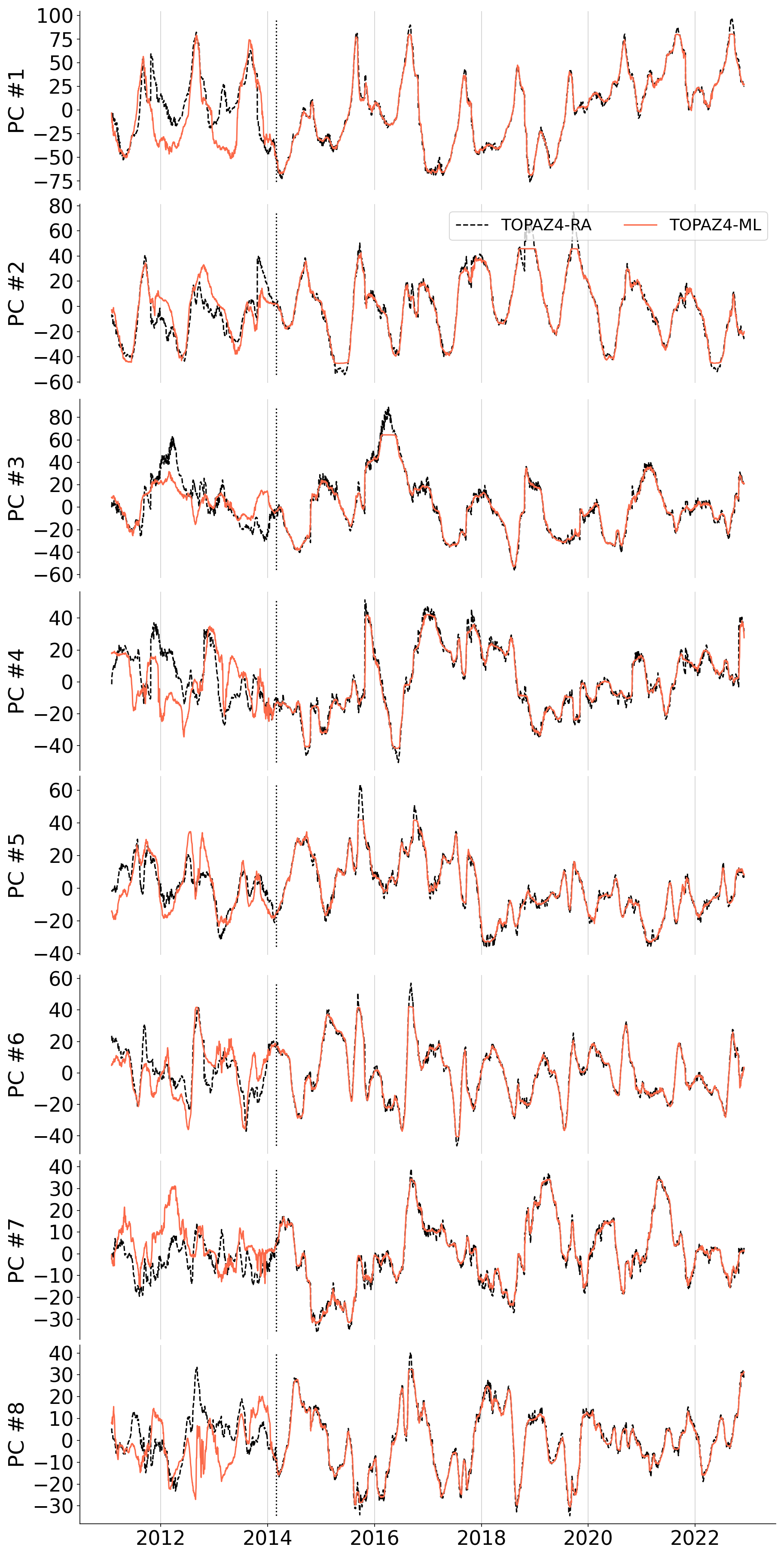
Figure A1 Time series of the principal component (PC) for each component in this study. TOPAZ4-RA (considered truth) and TOPAZ4-ML-predicted values are presented. A vertical line in 2014 indicates the separation of the test period from the training period.

Appendix B: Sea ice volume

Sea ice volume (Fig. B1) is obtained by multiplying the sea ice thickness by the area in each grid cell and by the sea ice concentration. It is then summed over the whole model domain. It is insensitive to high SIT values in areas of low ice concentration and is therefore a more convenient quantity than the average SIT to compare between models, although it is not as easily obtained from observations. For a clearer view of the decadal differences in sea ice thickness, refer to Supplement Fig. S9.

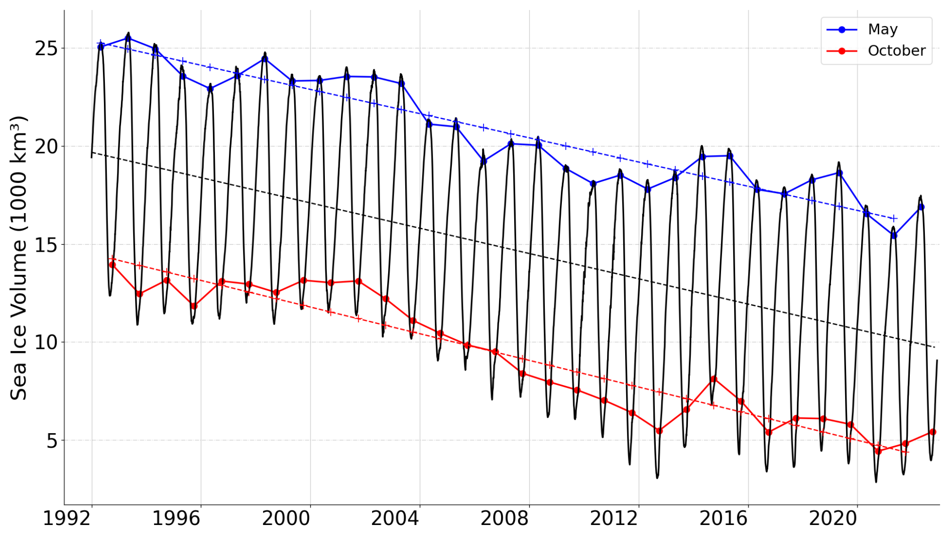
Figure B1 Total sea ice volume (1000 km³) for the entire Arctic domain from 1992 to 2022. The monthly average in May (October) is indicated in blue (red). Trends for the entire period are depicted by dotted lines. Note that the TOPAZ domain excludes the Pacific seas south of the Bering Strait.

Appendix C: Capability of the adjustment method as a function of sea ice thickness

To evaluate our method's performance across various sea ice thicknesses, we analyse the bias obtained from our method with the true bias as a function of the SIT (Fig. C1). Over the test period, our ML algorithm overestimates the adjustment (SIT bias difference is positive) for sea ice thickness between 3 and 5 m and underestimates the adjustment (SIT bias difference is negative) for thickness above 6 m.

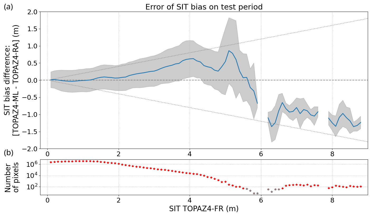
Figure C1 (a) The difference in bias correction between the ML prediction and the true bias correction as a function of the sea ice thickness from TOPAZ4-FR over the test period (2011–2013). The true bias correction is obtained from TOPAZ4-RA – TOPAZ4-FR. Bins of 10 cm are used to average the differences (blue) and their standard deviations (grey). The two diagonal lines represent 20 % of the sea ice thickness for each bin. Positive values indicate that the ML algorithm predicts an excessively high adjustment of sea ice thickness compared to the correction applied by the CS2SMOS data assimilation in TOPAZ4. (b) The number of pixels collected in each bin as a function of the sea ice thickness estimated by TOPAZ4-FR. Grey stars indicate bins with fewer than 50 pixels.