Doomed descent? How fast sulphate signals diffuse in the EPICA Dome C ice column

The loss of climate information due to smoothing of ionic impurity signals in ice provides a strong motivation for understanding their diffusion rates at ice-core sites. By analysing sulphate signals in the EPICA Dome C (EDC) core, recent studies estimated the vertical profile of effective diffusivity D_eff at that site. However, D_eff crudely approximates the local diffusivity D in the ice, it being a nonuniform-weighted average of D over large intervals. We formulate the mathematical inversion for retrieving the D profile from observed signals, which reconciles the findings of the earlier studies as well as elucidating the averaging approximation. Inversion for EDC sulphate reveals a rapid decrease in D through the firn layer – from ≈ 10⁻⁶ m² yr⁻¹ at the surface to ≈ 1.7 × 10⁻⁸ m² yr⁻¹ at the firn-ice transition (≈ 100 m depth, ≈ 2.5 ka), followed by a gradual decline to ≈ 10⁻¹⁰ m² yr⁻¹ through 100–2700 m (2.5–390 ka). This profile enables new interpretation of sulphate transport in the EDC column. We propose vapour diffusion of H₂SO₄ through interconnecting air pores as the cause of the high firn diffusivity. By evaluating the mechanisms controlling D below the firn (diffusion through ice crystals, liquid veins and grain boundaries and diffusion arising from interfacial motion), we infer a dominant partitioning of signals immediately below the firn to a connected vein system, and progressive smoothing of vein signals by Gibbs–Thomson diffusion down to ≈ 2000 m depth, which leaves more and more of the remaining signals to grain boundaries. We conclude that those sulphate signals that survive the initial fast diffusion in the firn to “punch through” to its base might survive into deep ice, and that EDC sulphate preserves a strongly filtered history of volcanic and climatic forcing that underrepresents changes and events shorter than a few years. For the Beyond EPICA – Oldest Ice and Million Year Ice Core drilling sites on Little Dome C, calculations assuming a diffusivity profile like our EDC profile and not exceeding 10⁻¹⁰ m² yr⁻¹ in ice older than 450 ka constrain the sulphate diffusion length in ice 1–2 Ma old to 2 cm at most, and probably as low as ≈ 1 cm, for atmospheric-sourced signals that experienced only diffusion and mechanical shortening in the column.

1 Introduction

Ionic impurities in ice cores provide valuable records of climate and environmental change (e.g. Legrand and Mayewski, 1997). The realisation that impurity signals in ice may be altered – not necessarily carrying climatic information “written in stone” – motivates study of the post-depositional processes threatening their integrity. Diffusion attenuates and broadens signals as they descend the ice column, potentially causing severe signal loss at depth, where the diffusion rate may be enhanced by higher temperature. The vertical pattern of the diffusion rate is of interest to questions about the reliability of ice-core ion records, the amount of climatic information retrievable from their signals, and the methods of reconstructing past forcings at the ice-sheet surface – questions that matter the more as ice-coring campaigns seek older and older records, such as in the Beyond EPICA – Oldest Ice project (BE-OI, 2017) and the Million Year Ice Core project (MYIC, 2020).

Recently, Fudge et al. (2024) and Rhodes et al. (2024) quantified diffusion on the high-resolution sulphate record of the EPICA (European Project for Ice Drilling in Antarctica) Dome C or “EDC” ice core (EPICA community members, 2004) from Antarctica. This record of sulphate concentration, measured by fast-ion chromatography (FIC) on bulk ice samples at ≈ 4 cm spacing down to 770 m depth and 1–2 cm spacing at greater depths (Traversi et al., 2002, 2009), is shown in Fig. 1a. By analysing how its signals vary along the core, together with a signal-evolution model that accounts for diffusion and vertical mechanical shortening of the ice, Fudge et al. (2024) and Rhodes et al. (2024) estimated the “effective diffusivity” D_eff of sulphate at EDC.

Sulphate is relevant in the diffusion context because volcanic events, which occur as sharp peaks on such records, provide data for synchronising ice-core timescales (e.g., Severi et al., 2012; Svensson et al., 2020) and inferring the history of volcanism – the record in Fig. 1a has been used to study eruption frequency back as far as 200 ka (Castellano et al., 2004; Lin et al., 2022; Wolff et al., 2023). Sulphate may also experience rapid transport in the liquid veins of polycrystalline ice, given the low eutectic temperature of sulphuric acid (−73 °C) implies its likely dissolution in vein water located at grain triple junctions (Mulvaney et al., 1988; Wolff et al., 1988; Nye, 1989; Mader, 1992), and given theoretical modelling which shows that ionic signals residing in a network of connected veins diffuse rapidly due to the Gibbs–Thomson effect (Ng, 2021). However, when studying impurity transport in ice, it is difficult to know how the bulk concentration of an ion partitions into contributions from different impurity sites – the ice-crystal lattice, grain boundaries, veins, and micro-inclusions; the mechanisms of impurity transfer between these sites also remain elusive (Barnes et al., 2003; Ng, 2021; Stoll et al., 2021). Thus, our understanding of how signals on the bulk concentration evolve is incomplete. Because the model used by Fudge et al. (2024) and Rhodes et al. (2024) in their diffusivity inversions tracks sulphate bulk concentration without resolving the partitioning, their effective diffusivity (D_eff) estimates for the EDC site reflect the overall outcome of different grain-scale transport processes. Yet, for this reason, their estimates provide global constraints on how these processes operate.

In this paper, we formulate a theory of diffusivity inversion that extends the methods of Fudge et al. (2024) and Rhodes et al. (2024), and which may be applied to other ions and to other ice cores besides EDC. Their studies referred to the “effective diffusivity” in part because of the caveat about impurity partitioning, but more specifically because their inversions assumed constant diffusivity acting on each signal as it evolves. Accordingly, they recognised D_eff as some weighted average of the true diffusivity. The averaging process has not been made clear though. We show mathematically that their D_eff estimates, owing to the averaging approximation, deviate significantly from the true diffusivity D (unless noted otherwise, all diffusivities in this paper pertain to sulphate). We improve upon their results to obtain the vertical profile of D in the EDC ice column, deriving new information about ionic impurity transport there. Notably, we discover high D values localised to the firn layer, whose cause is discussed towards the end. We also briefly consider what the findings mean for signal survivability at the sites of the BE-OI and MYIC projects. For convenience, we abbreviate Fudge et al. (2024) and Rhodes et al. (2024) as “F2024” and “R2024”, respectively, given how often they are referenced below.

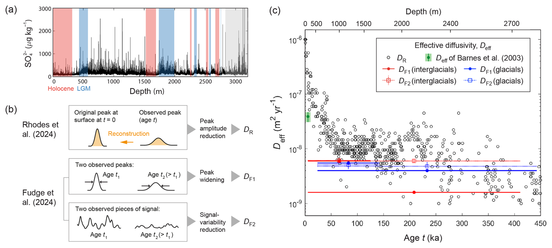
Figure 1 Approaches and results of the inversions for effective diffusivity D_eff by Fudge et al. (2024) and Rhodes et al. (2024), for sulphate at the EPICA Dome C ice-core site. (a) Depth profile of sulphate concentration from fast ion chromatography (Traversi et al., 2009), showing abundant peaks, many of them recording volcanic eruptions. Interglacial and glacial maximum periods are highlighted by red and blue shading, respectively; for their age and depth ranges, see Table A1 of Fudge et al. (2024). Grey shading marks the record > 2800 m, which is not studied herein. (b) Schematic of the approaches of Rhodes et al. (2024) and Fudge et al. (2024) for finding their D_eff estimates – D_R, D_F1, and D_F2, which are based on peak-amplitude decay, peak widening and signal-variability reduction, respectively. (c) Plot of their D_R, D_F1, and D_F2 results versus age back to 450 ka. The depth scale is indicated on the top axis. Horizontal bar shows the age range of each D_eff estimate, and vertical bar its uncertainty. Green point plots the D_eff estimate of Barnes et al. (2003) for the Holocene part of the record.

Figure 1 illustrates their diffusivity inversions. R2024's approach utilised the decay of signal peak amplitude, whereas F2024 employed two approaches, one based on signal peak widening and the other on the decay of signal variability down core (Fig. 1b). In R2024, 537 sulphate peaks were identified in the record down to ≈ 2800 m depth (0–450 ka). For each peak, the height of the corresponding original peak at deposition on the ice-sheet surface is reconstructed, by assuming that it held the same amount of sulphate as the observed peak (after removing local background concentration due to non-volcanic sources of sulphate such as marine biogenic emissions) and that it was Gaussian-shaped, with a duration of 3 years at “full width at tenth maximum” (FWTM), as is typically found for the width of volcanic sulphate peaks in Antarctic snow; see R2024 for detailed justification. Then, using their model, which we give in Eq. (1) below, R2024 numerically simulated the evolution of the reconstructed peak forward in time, tuning the diffusivity in multiple model runs to match the observed peak's height at its recorded age, to find D_eff for the peak. We denote by D_R their amplitude-based D_eff estimate.

In contrast, F2024 studied only signals in interglacial and glacial maximum periods (red and blue shading in Fig. 1a) and made separate inversions for these period types, to cater for the possibility of interglacial ice and glacial ice having different diffusivities. This is motivated by the idea that the different ice-column conditions (e.g. strain rate, mean crystal size) in these periods might affect impurity transport differently. Their width-based inversion, which gauges each peak's width by its “full width at half maximum” (FWHM), performs best-fit numerical simulations as R2024 did, but uses two peaks below the surface (Fig. 1b) rather than one peak and its reconstructed surface counterpart. Specifically, for interglacials and glacial maxima separately, they ran simulations to evolve a Gaussian signal with an initial width equal to the median width of observed peaks in the most recent period (either the Holocene or LGM) to match the median width of observed peaks in the earlier interglacials or glacial maxima, thus backing out D_eff for the intervening intervals. We denote by D_F1 their width-based D_eff estimate.

The other approach of F2024 uses a method pioneered by Barnes et al. (2003) for quantifying signal variations in terms of “mean absolute gradient” (explained in Sect. 2.3) to estimate D_eff from the decrease of signal variability down core. Using the method, Barnes et al. (2003) had estimated D_eff=3.9 ± 0.8 × 10⁻⁸ m² yr⁻¹ for the Holocene part (top 350 m) of the sulphate record in Fig. 1a. F2024 essentially applied the method to older parts of the core, focussing on the sequence of interglacials and glacial maxima. We denote by D_F2 their gradient-based D_eff estimate (Fig. 1b).

The effective diffusivities of R2024 and F2024 (Fig. 1c) show striking differences. Although D_R, D_F1 and D_F2 in the deeper record ≈ 200 to 450 ka (≈ 2100–2800 m) have similar magnitudes, ∼ 10⁻⁹–10⁻⁸ m² yr⁻¹, D_R is much higher (up to 10⁻⁶ m² yr⁻¹) than D_F1 and D_F2 in ice ≲ 50 ka, where it decays with age and depth. As R2024 reported, their median D_R value for Holocene ice (0–10 ka), 2.4 × 10⁻⁷ m² yr⁻¹, is nearly ten times the D_eff estimate of Barnes et al. (2003) (green data point in Fig. 1c). Beyond its initial decay, D_R averages at ≈ 10⁻⁸ m² yr⁻¹ in 50–200 ka, still about twice of D_F1 and D_F2. On seeing that D_F1 and D_F2 (≈ 5 × 10⁻⁹ m² yr⁻¹) are not much higher than the self-diffusivity of ice (≈ 3 × 10⁻¹⁰ to 3 × 10⁻⁹ m² yr⁻¹ at −50 to −35 °C; Ramseier, 1967), F2024 inferred that the fast signal diffusion in liquid veins modelled by Ng (2021) occurs only to a limited extent for sulphate in the upper ≈ 90 % of the ice column, and hence most sulphate there resides within ice crystals and at grain boundaries – not in the veins. On the other hand, R2024 interpreted the initial high (falling) D_R values for significant (diminishing) diffusion of sulphate in interconnected veins in the top quarter of the ice column.

Resolving these differences is imperative because the diffusivity profile is key to understanding how the crystal-scale diffusion mechanisms vary with depth and the factors involved, such as impurity partitioning. Besides adopting different inversion approaches, R2024 and F2024 processed the FIC data differently. R2024 only analysed sulphate peaks that are certainly volcanic by omitting others coincident with dust peaks, whereas F2024 applied the scaling procedure of Barnes et al. (2003) to the sulphate record to reduce the influence of background climate variations before extracting signals for analysis. These methodological differences can only explain minor discrepancies, not the overall incompatibility, between D_R and D_F1,2. The results in Fig. 1c also raise intriguing questions, notably the cause of the near-surface decay in D_R in ≈ 0–50 ka, which seems to continue through ≈ 100–450 ka at lower rate, and why (as both their studies pointed out) D_eff does not increase with depth, against the expectation that molecular diffusivity increases with temperature. The ice temperature at the EDC site increases monotonically from ≈ −53 °C at the surface to ≈ −12 °C at 2800 m (Fig. S1 in the Supplement).

Herein, our theory not only allows estimating the true diffusivity D, which is a more fundamental quantity than D_eff for probing impurity transport mechanisms; it also shows how the D_R, D_F1 and D_F2 estimates may be reconciled on account of their underlying averaging and two needed corrections in the D_F2 inversion. A key insight is that the signal-evolution model of F2024 and R2024 can be solved analytically, so the inversions can be done without numerical simulation. While our inversion results draw interest to the firn diffusivity, their signal-evolution model ignores firn densification; we therefore also examine its validity when used for inversions within the firn.

We focus on the EDC record in 0–2800 m (Fig. 1) by using the data collected by R2024 and F2024 without reprocessing the FIC sulphate concentrations. The record at depths > 2800 m (which features in part of F2024's study) is excluded for the reason given by R2024: there, some sulphate peaks may be non-volcanic and shaped by post-depositional processes other than diffusion and vertical mechanical shortening. This is shown by the presence of (i) anomalous peaks below 2800 m depth that have been chemically modified, as evidenced by ion association (Traversi et al., 2009), and (ii) other anomalous peaks starting from ≈ 2700 m (perhaps as shallow as 2500 m) that exhibit side troughs, indicating sulphate being “sucked” from neighbouring background levels towards zones with high cation concentration to form the peaks (Wolff et al., 2023). These artefacts reflect added complexity in the evolution of signals in deep ice at EDC that makes their origin uncertain. Our theory and analyses strictly concern signals without such artefacts, which give the ideal input data for diffusivity inversion. While R2024's data mitigate the issue by excluding potential artefact peaks during data collection, the deepest data of F2024 used by us may contain artefact signals, especially anomalous peaks of type (ii); but, for reasons explained later, this should not affect our conclusions.

2 Mathematical theory

2.1 Signal evolution

We begin with the advection–diffusion equation for signal evolution down the ice column, used by F2024 and R2024. In a coordinate frame moving with the ice, where z denotes distance below a material horizon descending towards the bed, signals in the bulk impurity concentration C(z,t) (measured in µg kg⁻¹, or µg L⁻¹ of meltwater) evolve according to

$$\begin{array}{}\text{(1)}& {\displaystyle \frac{\partial C}{\partial t}}=D\left(t\right){\displaystyle \frac{{\partial }^{\mathrm{2}}C}{\partial z^{\mathrm{2}}}}-{\dot{\mathit{\epsilon }}}_z\left(t\right)z{\displaystyle \frac{\partial C}{\partial z}}.\end{array}$$

Here, t is the age of the horizon, D is the impurity diffusivity, and ${\dot{\mathit{\epsilon }}}_z(<\mathrm{0})$ is local vertical strain rate. Equation (1) encapsulates the effects of mechanical shortening and diffusional spreading. Table A1 lists other mathematical symbols used in the paper.

Following F2024 and R2024, we use Eq. (1) to model sulphate signals, assuming an invariant strain-rate profile and constant surface accumulation rate at the core site – thus, a steady-state column with constant thickness and vertical velocity profile. In this system, signals travel through fields that are functions of depth in the column only, not time, so the age–depth scale allows translation between D(t) and its vertical profile. Material at age t has shortened from its original thickness at the surface by the thinning factor S, given by

$$\begin{array}{}\text{(2)}& S\left(t\right)=\exp \underset{\mathrm{0}}{\overset{t}{\int }}{\dot{\mathit{\epsilon }}}_z\left(\mathit{\eta }\right)\mathrm{d}\mathit{\eta },\end{array}$$

where η denotes the variable of integration. Differentiating Eq. (2) gives d$S/\mathrm{d}t={\dot{\mathit{\epsilon }}}_{z}S$. The thinning function S decays with age t from its value at the surface, $S_{\mathrm{0}}=S(t=\mathrm{0})$ = 1.

The inversion methods of R2024 and F2024 (elaborated in Sect. 2.2 and 2.3) use Eq. (1) as the basis, but as noted earlier, assume a constant D for each signal as it evolves down column. The resulting effective diffusivities D_R, D_F1 and D_F2 do not strictly represent the true (local) diffusivity D, instead averages measuring its cumulative effect over finite age and depth intervals; as we shall see, these intervals are large. By solving Eq. (1) analytically below, we develop exact inversions for D(t) that circumvent this assumption, at the same time deriving equations linking D(t) to D_R, D_F1 and D_F2. How Eq. (1) is affected by firn densification will be examined in Sect. 3.5, after we glimpse high firn diffusivity from our inversions.

2.2 Theory: peak-based inversions

2.2.1 The inversion possibility

A key property we exploit is that a Gaussian signal stays Gaussian under the combined mechanical shortening and diffusional spreading described by Eq. (1). F2024 and R2024 both initialised their simulations with Gaussian peaks, but did not harness this property. As alluded to by R2024, the sulphate flux from eruptions reaching the ice sheet often varies asymmetrically in time, but the deposited peaks rapidly relax to near-Gaussian. This motivates a Gaussian approximation to their shape.

To see the property, define the transformed depth

$$\begin{array}{}\text{(3)}& \mathit{\zeta }={\displaystyle \frac{z}{S\left(t\right)}}\end{array}$$

and define the variable

$$\begin{array}{}\text{(4)}& \mathit{\tau }\left(t\right)=\underset{\mathrm{0}}{\overset{t}{\int }}{\displaystyle \frac{D\left(\mathit{\eta }\right)}{S^{\mathrm{2}}\left(\mathit{\eta }\right)}}\mathrm{d}\mathit{\eta }+{\mathit{\tau }}_{\mathrm{0}},\end{array}$$

where τ₀ is the value of τ at zero age. Here, ζ is the destrained or unthinned thickness, and τ, an indirect proxy of age or time, accounts for the histories of diffusion and layer thinning. On letting $C(z,t)=f(\mathit{\zeta },\mathit{\tau })$, these changes of variable convert Eq. (1) to the classical heat equation

$$\begin{array}{}\text{(5)}& {\displaystyle \frac{\partial f}{\partial \mathit{\tau }}}={\displaystyle \frac{{\partial }^{\mathrm{2}}f}{\partial {\mathit{\zeta }}^{\mathrm{2}}}},\end{array}$$

which has the well-known (Gaussian) similarity solution

$$\begin{array}{}\text{(6)}& f(\mathit{\zeta },\mathit{\tau })\propto {\displaystyle \frac{\mathrm{1}}{\sqrt{\mathit{\tau }}}}{e}^{-{\mathit{\zeta }}^{\mathrm{2}}/\mathrm{4}\mathit{\tau }}.\end{array}$$

In the ζ-direction, this Gaussian's width expressed as a standard deviation is $\mathit{\sigma }=(\mathrm{2}\mathit{\tau }{)}^{\mathrm{1}/\mathrm{2}}$. Equations (5) and (6) mean that in τ–ζ space, signals experience uniform diffusion at unit rate, and a Gaussian peak decays in amplitude following the factor $\mathrm{1}/\sqrt{\mathit{\tau }}$ and widens following $\sqrt{\mathit{\tau }}$. Consequently, observations of peak widening or amplitude reduction down core, which provide data on τ(t), can be used to recover D(t) via Eq. (4). This idea forms the basis of the peak-based inversions.

For example, consider an amplitude-based inversion, where the “relative peak amplitude” (the ratio of a peak's observed amplitude to its original amplitude on deposition at the surface at t=0) has been compiled for different peaks along the core, as done by R2024. Suppose the relative amplitudes vary with age to trace out the function α(t). Then we have $\mathit{\alpha }\left(t\right)=\sqrt{{\mathit{\tau }}_{\mathrm{0}}/\mathit{\tau }}$ according to Eq. (6), and differentiating Eq. (4) with respect to t gives the inversion

$$\begin{array}{}\text{(7)}& D\left(t\right)=S^{\mathrm{2}}\left(t\right){\displaystyle \frac{\mathrm{d}\mathit{\tau }}{\mathrm{d}t}}=S^{\mathrm{2}}{\displaystyle \frac{\mathrm{d}}{\mathrm{d}t}}\left({\displaystyle \frac{{\mathit{\tau }}_{\mathrm{0}}}{{\mathit{\alpha }}^{\mathrm{2}}}}\right)=-{\displaystyle \frac{\mathrm{2}{\mathit{\tau }}_{\mathrm{0}}{S}^{\mathrm{2}}{\mathit{\alpha }}^{\prime }}{{\mathit{\alpha }}^{\mathrm{3}}}}\end{array}$$

(the ′ denotes derivative). This inversion requires the value ${\mathit{\tau }}_{\mathrm{0}}=\mathit{\tau }(t=\mathrm{0})$. For each observed peak, R2024 reconstructed the amplitude of the original peak by assuming it to be Gaussian, with a 3-year duration at FWTM and carrying the same total impurity load as the observed peak. They ignored firn densification effects and used the ice density in the reconstruction. We therefore set ${\mathit{\tau }}_{\mathrm{0}}={\mathit{\sigma }}^{\mathrm{2}}/\mathrm{2}$, with σ=3 years × $a/\mathrm{4.2919}$, where σ (m) is the standard deviation mentioned above, a is the ice-equivalent accumulation rate (m yr⁻¹), and the factor 4.2919 converts the FWTM of the Gaussian to σ. Positive τ₀ ensures a finite amplitude for the initial peak in Eq. (6). The differentiation in Eq. (7) assumes α to be smoothly varying; in practice, one fits a curve to the α-data prior to inversion.

Similarly, in a width-based inversion, where data on “relative peak width” (the ratio of observed width to original width) trace out the function β(t), such that $\mathit{\beta }\left(t\right)=\sqrt{\mathit{\tau }\left(t\right)S^{\mathrm{2}}\left(t\right)/{\mathit{\tau }}_{\mathrm{0}}{S}_{\mathrm{0}}^{\mathrm{2}}}=S\left(t\right)\sqrt{\mathit{\tau }\left(t\right)/{\mathit{\tau }}_{\mathrm{0}}}$, we derive

$$\begin{array}{}\text{(8)}& D\left(t\right)=S^{\mathrm{2}}\left(t\right){\displaystyle \frac{\mathrm{d}\mathit{\tau }}{\mathrm{d}t}}=S^{\mathrm{2}}{\displaystyle \frac{\mathrm{d}}{\mathrm{d}t}}\left({\displaystyle \frac{{\mathit{\tau }}_{\mathrm{0}}{\mathit{\beta }}^{\mathrm{2}}}{S^{\mathrm{2}}}}\right)=\mathrm{2}{\mathit{\tau }}_{\mathrm{0}}\mathit{\beta }({\mathit{\beta }}^{\prime }-\mathit{\beta }{\dot{\mathit{\epsilon }}}_z).\end{array}$$

Applying this inversion necessitates an assumption for the original peak width (for compiling β and τ₀). However, for comparing against the width-based inversion of F2024, Eq. (8) first needs to be adapted for use on two peaks below the surface, rather than one at the surface and one below (Fig. 1b). We attain the relevant result via a different route below.

2.2.2 Full-fledged theory

Before applying the above theory to data, we expand the mathematical analysis to unravel how peak-based inversions work and establish the relationship between D(t) and the effective diffusivities of F2024 and R2024.

The ratio $D/S^{\mathrm{2}}$ recurring in Eqs. (4), (7) and (8) relates a physical effect. As a signal shortens mechanically, its variations steepen, so it diffuses faster than if shortening were absent. With S<1 below the surface, $D/S^{\mathrm{2}}$ represents the amplified diffusivity. Another way of picturing this effect is to imagine the signal experiencing the diffusivity D, but over a longer time – longer by $\mathrm{1}/S^{\mathrm{2}}$ times. This motivates us to introduce another age variable, ψ, defined by dψ= d$t/S^{\mathrm{2}}\left(t\right)$. Specifically, we set ψ=0 at t=0, so that

$$\begin{array}{}\text{(9)}& \mathit{\psi }\left(t\right)=\underset{\mathrm{0}}{\overset{t}{\int }}{S}^{-\mathrm{2}}\left(\mathit{\eta }\right)\mathrm{d}\mathit{\eta }.\end{array}$$

This function has unit slope at t= 0 (since S(t=0) =1) and curves upward (e.g. Fig. 3c). We call ψ the dilated age because it accounts for thinning but excludes diffusion, unlike the proxy variable τ, which accounts for both.

On moving from t–z to ψ–ζ space (Fig. 2), the transformation z to ζ geometrically destrains the signal to track material horizons, whereas the transformation t to ψ stretches time to capture the mechanically-induced enhanced diffusion on the signal. With coordinate stretching absorbing both effects, the transformed signal obeys $\partial C/\partial \mathit{\psi }=D\left(\mathit{\psi }\right){\partial }^{\mathrm{2}}C/\partial {\mathit{\zeta }}^{\mathrm{2}}$ without a shortening term (Fig. 2b). Crucially, under the move, Eq. (4) is converted to

$$\begin{array}{}\text{(10)}& \mathit{\tau }\left(\mathit{\psi }\right)=\underset{\mathrm{0}}{\overset{\mathit{\psi }}{\int }}D\left(\mathit{\psi }\right)\mathrm{d}\mathit{\psi }+{\mathit{\tau }}_{\mathrm{0}},\end{array}$$

which shows that inversion for D fundamentally involves

$$\begin{array}{}\text{(11)}& D\left(\mathit{\psi }\right)={\displaystyle \frac{\mathrm{d}\mathit{\tau }}{\mathrm{d}\mathit{\psi }}}.\end{array}$$

In other words, as a Gaussian peak evolves in ψ–ζ space, its unthinned width squared and its inverse squared amplitude (recall that unthinned width $\propto \sqrt{\mathit{\tau }}$ and amplitude $\propto \mathrm{1}/\sqrt{\mathit{\tau }})$ increase at a rate with respect to ψ that equals the instantaneous or local diffusivity. Equivalently, the local diffusivity is given by the rate of change of these peak-form parameters with respect to dilated age ψ (Fig. 2b). Not surprisingly, the age-domain inversions in Eqs. (7) and (8) also involve rates of change.

Figure 2 Evolution of a Gaussian signal in (a) t–z space and (b) ψ–ζ space. Solid black curves signify material trajectories. Dashed curve in (b) marks the unthinned signal width, whose square increases at a rate with respect to ψ that reflects the instantaneous diffusivity.

Given these insights, we can calculate the effective diffusivities D_R and D_F1 of R2024 and F2024 analytically, which obviates need to integrate Eq. (1) numerically and perform multiple simulations to fit data. As noted before, their inversions assumed constant D during each signal's descent. If Eq. (10) is used to reproduce their inversions, then we set D ≡D_eff (constant) in its integral, which gives

$$\begin{array}{}\text{(12)}& \mathit{\tau }\left(\mathit{\psi }\right)=D_{\mathrm{eff}}\mathit{\psi }+{\mathit{\tau }}_{\mathrm{0}},\end{array}$$

or

$$\begin{array}{}\text{(13)}& D_{\mathrm{eff}}={\displaystyle \frac{\mathit{\tau }-{\mathit{\tau }}_{\mathrm{0}}}{\mathit{\psi }}}={\displaystyle \frac{{\mathit{\tau }}_{\mathrm{0}}}{\mathit{\psi }}}\left({\displaystyle \frac{\mathit{\tau }}{{\mathit{\tau }}_{\mathrm{0}}}}-\mathrm{1}\right),\end{array}$$

which describes the inversion based on a subsurface peak and its reconstructed original (surface) peak. Where the inversion uses a pair of subsurface points, say, τ₁ at dilated age ψ₁ and τ₂ at dilated age ψ₂, differencing the application of Eq. (12) to these data yields

$$\begin{array}{}\text{(14)}& D_{\mathrm{eff}}={\displaystyle \frac{{\mathit{\tau }}_{\mathrm{2}}-{\mathit{\tau }}_{\mathrm{1}}}{{\mathit{\psi }}_{\mathrm{2}}-{\mathit{\psi }}_{\mathrm{1}}}}.\end{array}$$

From these results, it follows that the R2024 inversion is equivalent to

$$\begin{array}{}\text{(15)}& D_{\mathrm{R}}\left(t\right)={\displaystyle \frac{{\mathit{\tau }}_{\mathrm{0}}}{\mathit{\psi }\left(t\right)}}\left({\displaystyle \frac{\mathrm{1}}{{\mathit{\alpha }}^{\mathrm{2}}\left(t\right)}}-\mathrm{1}\right),\end{array}$$

with ψ given by Eq. (9) and the data for α and τ₀ gathered as before (Sect. 2.2.1), whereas the width-based inversion of F2024 for two peaks of age t₁ and t₂ has the analytical counterpart

$$\begin{array}{}\text{(16)}& D_{\mathrm{F}\mathrm{1}}={\displaystyle \frac{\mathit{\tau }\left(t_{\mathrm{2}}\right)-\mathit{\tau }\left(t_{\mathrm{1}}\right)}{\mathit{\psi }\left(t_{\mathrm{2}}\right)-\mathit{\psi }\left(t_{\mathrm{1}}\right)}},\end{array}$$

in which the τ values derive from observed peak widths. F2024 measured the unthinned FWHM of each peak, so $\mathit{\tau }={\mathit{\sigma }}^{*\mathrm{2}}/\mathrm{2}$, where ${\mathit{\sigma }}^{*}=$ FWHM/2.3548 is the destrained standard deviation of the Gaussian.

The effective diffusivity from Eq. (15) or (16) is valid for the specific interval bracketed by the paired data, as in R2024 and F2024's simulation-based inversions. The interval in R2024's inversion spans each peak's entire history. In F2024's inversion, which uses paired data between the Holocene and earlier interglacials or between the LGM and earlier glacial maxima, the intervals exceed ∼ 100 kyr. Thus, D_R of R2024 and D_F1 of F2024 are effective diffusivity estimates for different periods – this is a key reason behind their discrepancy, which we will point out again when analysing results in Sect. 3.

Next we relate the effective diffusivities to the true diffusivity D(t). Applying Eq. (10) to paired data (ψ₁, τ₁) and (ψ₂, τ₂), eliminating τ₀, and using Eq. (14), yields

$$\begin{array}{}\text{(17)}& D_{\mathrm{eff}}={\displaystyle \frac{\mathrm{1}}{{\mathit{\psi }}_{\mathrm{2}}-{\mathit{\psi }}_{\mathrm{1}}}}\underset{{\mathit{\psi }}_{\mathrm{1}}}{\overset{{\mathit{\psi }}_{\mathrm{2}}}{\int }}D\left(\mathit{\psi }\right)\mathrm{d}\mathit{\psi },\end{array}$$

or

$$\begin{array}{}\text{(18)}& D_{\mathrm{eff}}\left(\mathit{\psi }\right)={\displaystyle \frac{\mathrm{1}}{\mathit{\psi }}}\underset{\mathrm{0}}{\overset{\mathit{\psi }}{\int }}D\left(\mathit{\psi }\right)\mathrm{d}\mathit{\psi }\end{array}$$

if the upper data point lies at the surface. These results show that D_eff is the interval average of D, not over t but over the dilated age ψ. Since ψ(t) curves upward (Fig. 3c), D_eff is biased towards D in the older part of the averaging interval; but it is influenced by D in the younger part. The larger is the interval, the more crudely D_eff approximates D at the lower (deeper) data point.

Equation (18) leads to further insights on the profile D_R(t) retrieved by the R2024 inversion. By evaluating its integral, working with time rather than ψ as the integration variable, we derive

$$\begin{array}{}\text{(19)}& \begin{array}{rl}{D}_{\mathrm{R}}\left(t\right)& ={\displaystyle \frac{\mathrm{1}}{\mathit{\psi }\left(t\right)}}\underset{\mathrm{0}}{\overset{t}{\int }}D\left(\mathit{\eta }\right){\mathit{\psi }}^{\prime }\left(\mathit{\eta }\right)\mathrm{d}\mathit{\eta }\\ & =D\left(t\right)-{\displaystyle \frac{\mathrm{1}}{\mathit{\psi }\left(t\right)}}\underset{\mathrm{0}}{\overset{t}{\int }}{D}^{\prime }\left(\mathit{\eta }\right)\mathit{\psi }\left(\mathit{\eta }\right)\mathrm{d}\mathit{\eta }.\end{array}\end{array}$$

According to this expression, D_R found from an observed peak not only reflects the local diffusivity D at its depth, but also inherits a signal from the variations in D throughout its earlier shallower history: we call this the “memory effect”. Notably, D_R(t) overestimates (underestimates) D(t) if D(t) is a decreasing (increasing) function.

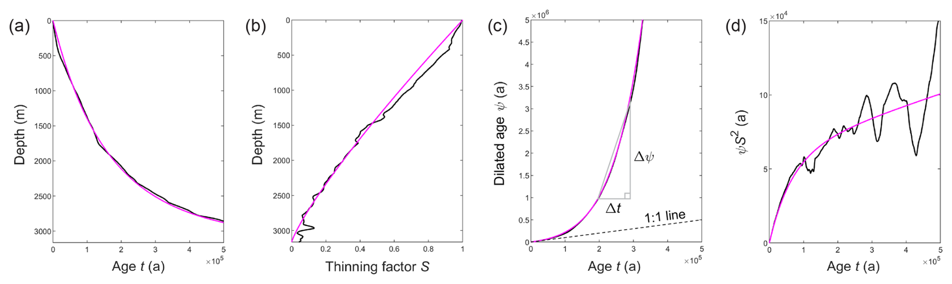
Figure 3 Functions used in our diffusivity inversions for the EPICA Dome C ice-core site: (a) the AICC2012 age–depth scale (Bazin et al., 2013; Veres et al., 2013) and the corresponding (b) depth profile of thinning factor S, (c) dilated age ψ versus age t, and (d) ψS² versus age. Black curves derive directly from the AICC2012 scale. Magenta curves, used in our inversions, are smooth approximations based on an ice-flow model assuming the submergence velocity $w_i=a_{\mathrm{s}}(h/H{)}^{\mathrm{1.2}}$, where h is height above the bed, H=3165 m (mean ice thickness chosen by Rhodes et al., 2024), and surface accumulation rate a_s=0.0195 m yr⁻¹. Grey triangle in (c) illustrates the misamplification factor (Sect. 2.3).

Differentiating the first equation in Eq. (19) gives the opposite conversion from D_R to D,

$$\begin{array}{}\text{(20)}& D\left(t\right)={\displaystyle \frac{\mathrm{1}}{{\mathit{\psi }}^{\prime }}}{\displaystyle \frac{\mathrm{d}}{\mathrm{d}t}}\left[\mathit{\psi }{D}_{\mathrm{R}}\right(t\left)\right]=D_{\mathrm{R}}+D_{\mathrm{R}}^{\prime }\mathit{\psi }{S}^{\mathrm{2}},\end{array}$$

which shows that D is less (greater) than D_R wherever D_R decreases (increases) down core. R2024 recognised D_R as a “time-weighted diffusivity” and took care when interpreting their D_R(t) profile; but without the analytical result in Eq. (20), inferring D from D_R is challenging. The present analysis also reveals the weighting to be highly nonlinear. In Sect. 3, we use Eq. (20) to estimate D(t) from D_R(t) and Eq. (19) to predict D_R(t) from D(t), discovering a marked difference between these curves.

2.3 Theory: gradient-based inversion

We turn to F2024's inversion for the effective diffusivity D_F2, which calculates the “mean absolute gradient” $\overline{m}$ of signals with the Barnes et al. (2003) method, which in turn is based on the diffusion-length theory of Johnsen (1977). We extend this framework to derive an exact inversion for D from $\overline{m}$, exposing the averaging approximation behind D_F2. We find that the Barnes et al. (2003) method – and thus the D_F2 estimates – require two corrections.

In the Barnes et al. (2003) method, the concentration record C is first destrained and processed to suppress unwanted signals from background climate variations. Signal peaks on the processed record, C_p, are thought to reflect the sulphate input from volcanic events more reliably (with less bias) than C. To quantify the signal variability on C_p, they studied different 10 m long sections down core by calculating their signal mean absolute gradient,

$$\begin{array}{}\text{(21)}& \overline{m}={\displaystyle \frac{\mathrm{1}}{n\mathrm{\Delta }\mathit{\zeta }}}\sum _{i=\mathrm{1}}^n\left|C_{p,i+\mathrm{1}}-C_{\mathrm{p},i}\right|,\end{array}$$

where C_p,i denotes individual processed concentration measurements, Δζ is the destrained interval between measurements, and n is the number of intervals in each 10 m. Equation (21) is the same as their Eq. (1), despite written with different symbols.

Their method quantifies the rate of diffusive smoothing by using the observed decrease in $\overline{m}$ down core (Fig. 1b) and retrieves D_eff from the rate. Notably, they regard the principal signals on C_p as periodic, with a wavenumber k^* that does not vary with depth on the destrained record (we use ^* to signify destraining). Accordingly, the ratio of $\overline{m}$ of a core section at depth to the mean absolute gradient ${\overline{m}}_{\mathrm{0}}$ of a reference section higher in the column measures the amplitude decay of the signals, and they equate this ratio to the signal attenuation predicted for Eq. (1) by Johnsen (1977) – thus,

$$\begin{array}{}\text{(22)}& {\displaystyle \frac{\overline{m}}{{\overline{m}}_{\mathrm{0}}}}=\exp (-k^{\ast \mathrm{2}}{\mathit{\sigma }}^{\ast \mathrm{2}}/\mathrm{2}),\end{array}$$

in which σ^* is the destrained value of the diffusion length σ; that is, ${\mathit{\sigma }}^{*}=\mathit{\sigma }/S\left(t\right)$.

In Johnsen's theory, the diffusion length σ evolves according to the ordinary differential equation

$$\begin{array}{}\text{(23)}& {\displaystyle \frac{\mathrm{d}{\mathit{\sigma }}^{\mathrm{2}}}{\mathrm{d}t}}=\mathrm{2}D\left(t\right)+\mathrm{2}{\dot{\mathit{\epsilon }}}_z\left(t\right){\mathit{\sigma }}^{\mathrm{2}},\end{array}$$

and transforming this to the destrained coordinate system yields

$$\begin{array}{}\text{(24)}& \mathrm{d}{\mathit{\sigma }}^{*\mathrm{2}}/\mathrm{d}t=\mathrm{2}D\left(t\right)/S^{\mathrm{2}}\left(t\right).\end{array}$$

However, Barnes et al. (2003) took $\mathrm{d}{\mathit{\sigma }}^{*\mathrm{2}}/\mathrm{d}t=\mathrm{2}D$ without the final $\mathrm{1}/S^{\mathrm{2}}$, assuming Eq. (23) with ${\dot{\mathit{\epsilon }}}_z$ set to zero to be a valid diffusion-length equation for unthinned records. On taking a constant (effective) diffusivity, they then found ${\mathit{\sigma }}^{*\mathrm{2}}=\mathrm{2}{D}_{\mathrm{eff}}t$, which, together with Eq. (22), led them to the inversion formula

$$\begin{array}{}\text{(25)}& D_{\mathrm{eff}}=-{\displaystyle \frac{\mathrm{1}}{k^{\ast \mathrm{2}}t}}\ln \left({\displaystyle \frac{\overline{m}}{{\overline{m}}_{\mathrm{0}}}}\right).\end{array}$$

When rewritten for a pair of subsurface data points, this gives the F2024 inversion formula:

$$\begin{array}{}\text{(26)}& D_{\mathrm{F}\mathrm{2}}=-{\displaystyle \frac{\mathrm{1}}{k^{\ast \mathrm{2}}(t_{\mathrm{2}}-t_{\mathrm{1}})}}\ln \left({\displaystyle \frac{{\overline{m}}_{\mathrm{2}}}{{\overline{m}}_{\mathrm{1}}}}\right).\end{array}$$

These formulas are approximate because of the missing $\mathrm{1}/S^{\mathrm{2}}$ in the underlying diffusion-length model: strictly, Eq. (24) should be used instead. In particular, for the EDC core site, the approximation is reasonable for signals in t≲10⁴ years (because S≈1 up to that age; Fig. 3a, b) but not beyond. It follows that the D_eff estimate of Barnes et al. (2003) for the Holocene ice (Fig. 1c) is approximately valid, but the D_F2 estimates of F2024 for older sections of ice suffer large inaccuracies.

Having explained the Barnes et al. method, we modify it to derive an exact inversion for D. In the ψ–ζ coordinate system, Johnsen's diffusion-length equation (Eqs. 23 or 24) takes the form¹

$$\begin{array}{}\text{(27)}& {\displaystyle \frac{\mathrm{d}{\mathit{\sigma }}^{\ast \mathrm{2}}}{\mathrm{d}\mathit{\psi }}}=\mathrm{2}D\left(\mathit{\psi }\right),\end{array}$$

and substituting for σ^*2 from Eq. (22) gives

$$\begin{array}{}\text{(28)}& D\left(\mathit{\psi }\right)=-{\displaystyle \frac{\mathrm{1}}{k^{\ast \mathrm{2}}}}{\displaystyle \frac{\mathrm{d}\left(\ln \overline{m}\right)}{\mathrm{d}\mathit{\psi }}}.\end{array}$$

This inversion formula involves a rate of change, as in the peak-based inversions, and shows that D can be estimated from the slope of the logarithmic plot of $\overline{m}$ versus dilated age ψ (we will explore this with EDC data in Sect. 3.3).

One can again relate the effective diffusivity to D. Suppose D in Eq. (27) equals a constant, D_E; this is the effective diffusivity that is found by the inversion without the approximation of Barnes et al. (2003) described above. Then ${\mathit{\sigma }}^{*\mathrm{2}}=\mathrm{2}{D}_{\mathrm{E}}\mathit{\psi }$. Using this together with Eq. (22) for paired data leads to the inversion formula

$$\begin{array}{}\text{(29)}& \begin{array}{rl}{D}_{\mathrm{E}}& =-{\displaystyle \frac{\mathrm{1}}{k^{\ast \mathrm{2}}({\mathit{\psi }}_{\mathrm{2}}-{\mathit{\psi }}_{\mathrm{1}})}}\ln \left({\displaystyle \frac{{\overline{m}}_{\mathrm{2}}}{{\overline{m}}_{\mathrm{1}}}}\right)\\ & (\equiv {\displaystyle \frac{\mathrm{1}}{{\mathit{\psi }}_{\mathrm{2}}-{\mathit{\psi }}_{\mathrm{1}}}}\underset{{\mathit{\psi }}_{\mathrm{1}}}{\overset{{\mathit{\psi }}_{\mathrm{2}}}{\int }}D(\mathit{\psi }\left)\mathrm{d}\mathit{\psi }\right).\end{array}\end{array}$$

We see that D_E is the average of D over the dilated age ψ, as for D_R and D_F1. On comparing D_E against the effective diffusivities in Eqs. (25) and (26), we find

$$\begin{array}{}\text{(30)}& D_{\mathrm{F}\mathrm{2}}={\displaystyle \frac{{\mathit{\psi }}_{\mathrm{2}}-{\mathit{\psi }}_{\mathrm{1}}}{t_{\mathrm{2}}-t_{\mathrm{1}}}}{D}_{\mathrm{E}},\end{array}$$

which means that D_F2 of F2024 (also D_eff of Barnes et al. 2003) is misamplified by (${\mathit{\psi }}_{\mathrm{2}}-{\mathit{\psi }}_{\mathrm{1}})/(t_{\mathrm{2}}-t_{\mathrm{1}}$) and strongly overestimates the effective diffusivity in deep intervals (see triangle in Fig. 3c). The issue stems from the missing $\mathrm{1}/S^{\mathrm{2}}$. The misamplification ratio allows the effective diffusivities of Barnes et al. (2003) and F2024 to be corrected to give the desired value, D_E.

The other correction in the mean absolute gradient approach concerns the signal wavenumber k^*. Barnes et al. (2003) and F2024 estimated it via $k^{*}=\mathrm{2}\mathit{\pi }/\overline{w}$, where the mean destrained wavelength $\overline{w}$ of the signals is found by calculating

$$\begin{array}{}\text{(31)}& \overline{w}={\displaystyle \frac{\mathrm{4}}{\overline{m}L}}\sum _{i=\mathrm{1}}^n\left|C_{\mathrm{p},i}-{\overline{C}}_{\mathrm{p}}\right|\mathrm{\Delta }\mathit{\zeta }\end{array}$$

for a long record (F2024 used the Holocene or LGM part of the EDC record for this); L is the length of the record and ${\overline{C}}_{\mathrm{p}}$ its mean impurity concentration. Barnes et al. (2003) idealised the signals as triangular-shaped when deriving Eq. (31), but our repeat derivation in Appendix B shows that its right-hand side should be doubled, or π/2 times larger if one assumes sinusoidal signals. Consequently, their method overestimates k^* by ≈ 1.6–2 times, and the D_F2 estimates of F2024 and the D_eff estimate of Barnes et al. (2003) for Holocene ice (3.9 ± 0.8 × 10⁻⁸ m² yr⁻¹) are too small by a factor of $k^{*\mathrm{2}}\approx \mathrm{2}$.5–4 times. In our D_F2 inversions below, we remedy both issues by correcting the results with this factor and the misamplification ratio.

3 Diffusivity inversions: results and analysis

We proceed to estimate the true diffusivity profile D(t) at the EDC site, using the theory of Sect. 2 and data from F2024 and R2024 as input. The work is done in stages. In Sect. 3.1, 3.2, and 3.3, we undertake inversions from peak amplitude, peak width, and signal gradient in turn, exploring avenues including the conversion of D_eff to D and direct inversion of data, as well as finding the effective diffusivities D_R, D_F1 and D_F2 with analytical formulas. While these sections allow gleaning information about D(t), we further constrain its form by forward modelling in Sect. 3.4. In Sect. 3.5, after inferring high sulphate diffusivity confined to the firn layer, we examine how firn densification impacts the diffusivity inversion.

F2024 and R2024 used the AICC2012 chronology of the EDC site (Fig. 3a; Bazin et al., 2013; Veres et al., 2013) throughout data compilation and analyses. To maximise compatibility of our results with theirs, we employ the same chronology, rather than the newer AICC2023 chronology (Bouchet et al., 2023). In particular, our inversions use what we call “AICC2012-based” functions – smoothed forms of the thinning factor S and dilated age ψ(t) (Fig. 3, magenta curves), which we derive from a power-law model of the ice submergence velocity in the EDC column fitted to the AICC2012 age–depth scale; see the caption of Fig. 3 for the details. Although the smoothing injects minor differences between our D_eff estimates and those of R2024 and F2024, it is desirable because the thinning function provided with the AICC2012 dataset is non-monotonic (black curve, Fig. 3b), with small bumps that imply negative strain rate at various depths.

3.1 Inversions from peak-amplitude decay

Figure 4a shows the relative amplitudes α of the peaks studied by R2024, obtained from their Supplementary data by dividing observed peak heights by original peak heights. The values show considerable scatter but generally decay with age.

To compute the effective diffusivity D_R for each peak, we apply Eq. (15) to its α-value, setting τ₀ as described in Sect. 2.2.1. When calculating the strain rate ${\dot{\mathit{\epsilon }}}_z$ for simulating Eq. (1), R2024 adopted an ice submergence velocity profile derived not from the AICC2012 scale, instead from a Nye model with an ice thickness of 3165 m and a surface accumulation rate that puts the peak at its observed depth, so that its age and depth agree with the AICC2012 scale. Thus, their inversion of D_R envisages a slightly different steady-state ice column for each peak. Their use of the Nye model, which does not resolve the details of firn compaction near the top of the column, seems consistent with their choice of working with ice-equivalent depths when compiling original peak amplitudes (Sect. 2.2.1). We shall say more about the effect of the firn processes in Sect. 3.5.

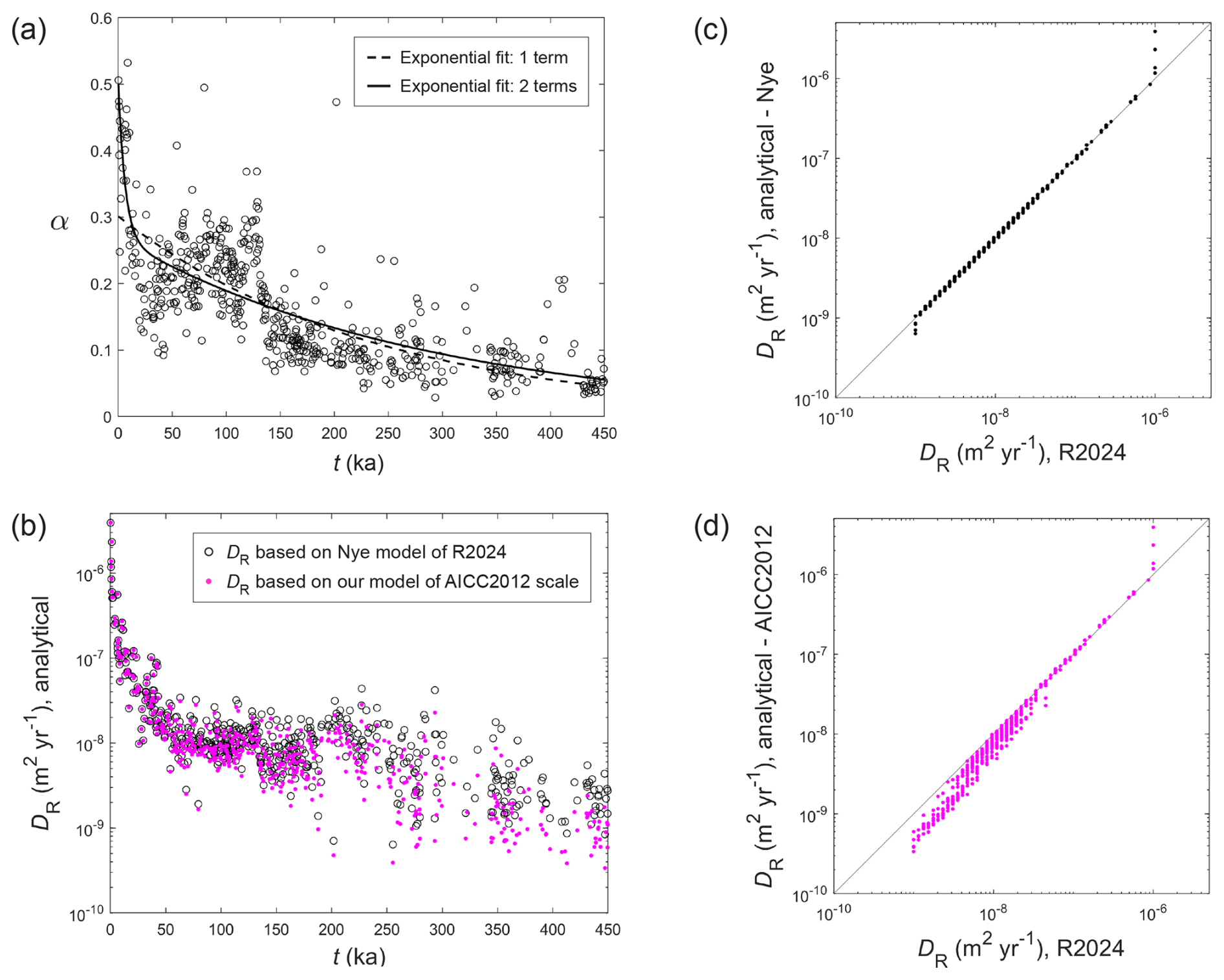
Figure 4 Analytical inversion for the effective diffusivity D_R from the peak-amplitude data of Rhodes et al. (2024). (a) Amplitude ratio α versus age t for 537 peaks. Dashed curve plots best-fit exponential $\mathit{\alpha }\left(t\right)=\mathrm{0.301}\exp (-\mathrm{4.22}$ × 10⁻³t); solid curve, best-fit exponential sum $\mathit{\alpha }\left(t\right)=\mathrm{0.232}\exp (-\mathrm{0.157}t)+\mathrm{0.268}\exp (-\mathrm{3.49}\times {\mathrm{10}}^{-\mathrm{3}}t)$. (b) Computed D_R values versus age. Black circles plot results of the inversion assuming the Nye model of Rhodes et al. (2024); magenta points plot results of the inversion assuming our AICC2012-based ice-flow functions in Fig. 3. Following Rhodes et al. (2024), each D_R value is plotted at the age of the observed peak, rather than as a bar spanning the period over which it applies. (c) Scatterplot of the black-circled D_R values in (b) against the D_R estimates of Rhodes et al. (2024), which they found by simulating Eq. (1) to match peak-amplitude decay. (d) Scatterplot of the magenta D_R values in (b) against the D_R estimates of Rhodes et al. (2024).

To show that our analytic approach can reproduce the D_R estimates of R2024, in our first use of Eq. (15) we adopt their ice-flow approximation by using ψ(t) based on their peak-specific Nye model instead of our AICC2012-based model. The corresponding D_R results (Fig. 4b, circles) agree closely with their estimates (Fig. 1c), decaying from ∼ 10⁻⁶ to ∼ 10⁻⁹ m² yr⁻¹, rapidly in ≈ 0–50 ka and slowly beyond. We find four values exceeding 10⁻⁶ m² yr⁻¹ near t=0 and four values below 10⁻⁹ m² yr⁻¹ not reported by R2024 (Fig. 4c and b). These and other minor discrepancies between our results arise because Eq. (15) is an exact formula for D_R, whereas their D_R estimates are constrained to 50 graded values (visible from the banding in Fig. 4c) on the log scale between 10⁻⁹ and 10⁻⁶ m² yr⁻¹ (values outside these bounds are clipped to them).

Performing the same inversion with our AICC2012-based function ψ(t) (Fig. 3c) yields lower D_R estimates, especially for deeper peaks (Fig. 4b and d, magenta points). This is because their Nye model tends to overestimate S (underestimate the amount of thinning) at depth; less of the thinning-induced enhancement in signal diffusion (Sect. 2.2.2) is captured, making their D_R estimates larger. The lowering helps explain some of the difference between D_R and F2024's D_eff estimates.

Next, we attempt to estimate the true diffusivity profile D(t) by two approaches. The first applies the time-domain inversion in Eq. (7) (same as Eq. (11) in the ψ–ζ domain) to a smoothed version of α, which we derive by fitting the α-data with the sum of two exponentials (solid curve, Fig. 4a). This function is preferred to a single exponential (dashed curve, Fig. 4a) because it captures the high α-values near t=0 better. In Eq. (7) we use the AICC2012-based thinning function S (Fig. 3b).

The second approach converts D_R to D with Eq. (20), assuming the AICC2012-based function ψS² (Fig. 3d). To derive a smooth input for Eq. (20), in which the derivative $D_{\mathrm{R}}^{\prime }$ appears, we spline-fit our AICC2012-based D_R estimates from Fig. 4b on log-10 scale. These estimates show pronounced fluctuations and scatter on time scales shorter than ≈ 20 kyr that indicate uncertainty and noise on the relative amplitudes α, so we choose a level of spline smoothing to suppress these fluctuations; see Spline 2 in Fig. 5b, e, h. However, the exact time scales on which fluctuations in D_R reflect true changes in diffusivity is unknown, so we experiment also with less and more smoothing by using Spline 1 and Spline 3 (the left-hand and right-hand columns of panels in Fig. 5). Spline 3 strongly suppresses fluctuations in D_R shorter than about 50 kyr.

The curves of D(t) computed by this second approach (Fig. 5, solid black curves) indicate high, steeply-decaying diffusivity in the first ≈ 2 to 8 ka – from ∼ 10⁻⁶ m² yr⁻¹ to well below 10⁻⁷ m² yr⁻¹, followed by generally low diffusivity beyond (∼ 10⁻⁸ m² yr⁻¹) and even negative diffusivity in some age ranges (see comments below). Although stronger spline smoothing lengthens the initial fast decay, all three curves portray D as greatly diminished from its surface value by several ka (Fig. 5d–i). Because the firn-ice transition at EDC lies at ≈ 100 m depth (e.g. Landais et al., 2006; Calonne et al., 2022), where t≈ 2.5 ka, much of the initial steep drop in D apparently occurs in the firn layer; we explore the cause of this later in Sect. 4.1. In contrast, D(t) retrieved by the first approach (Fig. 5, dashed black curve in all panels) shows a much more subdued decay over the first 30 ka, starting from a lower surface diffusivity ≈ 6 × 10⁻⁸ m² yr⁻¹. We think that this is because the two-term exponential in Fig. 4a does not adequately capture the high negative slope of the α-data near t=0, which is necessary for Eq. (7) to reconstruct the details of D there.

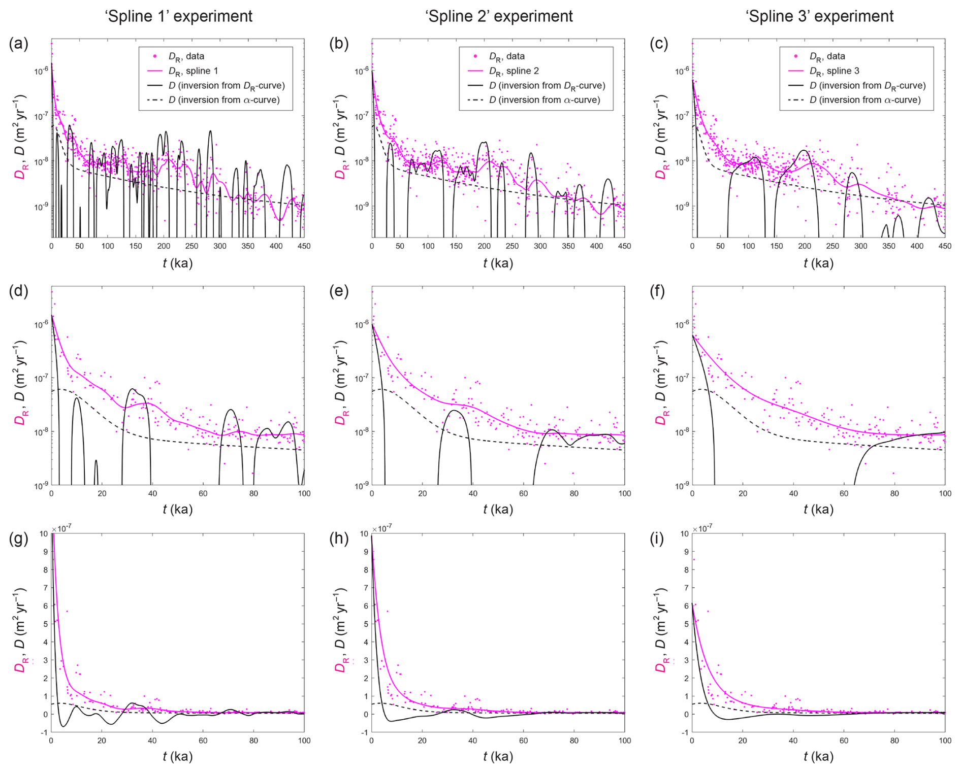
Figure 5 Analytical inversions for D(t) from D_R. The left, middle, and right columns of panels document three different experiments where the curves of D_R serving as input to the inversion (“Splines 1, 2 and 3”; magenta curves) have been derived by spline-fitting the D_R point data at different smoothness. The level of spline smoothing increases from left to right. In each panel, magenta circles plot the D_R data from Fig. 4b; black curve shows D(t) obtained by using Eq. (20) with the chosen spline for D_R; dashed black curve shows D(t) obtained by using Eq. (7) with the two-term exponential curve of α in Fig. 4a as input. Each row of panels displays results on the same axes: (a–c) over 450 ka; (d–f) over the last 100 ka in log scale; (g–i) over the last 100 ka in linear scale.

In the second approach, the curves of D(t) lie below the D_R estimates in many places. As expected from our theory in Sect. 2.2.2, D(t) lies above (below) the spline curve of D_R where this curve rises (drops). Where D_R increases with age, high D (> D_R) is retrieved because peaks with much lower amplitude than overlying peaks in the column imply high diffusivity in the intervening depth interval. Where D_R decreases with age, low D (< D_R) is retrieved because peaks with undiminished (or higher) amplitudes compared to overlying peaks can be explained only by low (or negative) diffusivity in the intervening interval. In this connection, a robust feature of all three curves of D(t) is that they and their initial steep drops lie well below the curves of D_R in the first few tens of ka, where the D_R estimates decay much more gradually (Fig. 5d–i). This feature, which remains if we use the D_R values of R2024 as input to the conversion, implies that D_R contains a long memory of the initial high diffusivities. We anticipated this memory effect in Sect. 2.2.2. Here, it operates because the effective diffusivity D_R “remembers” the initial rapid lowering of the peaks by fast diffusion during their first few thousand years of evolution, which cannot be undone however slow is diffusion afterwards. This finding is supported by the relative amplitudes in Fig. 4a, which evidence more than 40 % reduction in peak height (α<0.6) on even the shallowest peaks.

The second inversion approach is not without limitations. First, the real original sulphate peaks at the surface might have durations (FWTMs) different from the 3 years assumed in the inversion and durations different from each other, as shown by the large scatter in the α and D_R values. Second, the level of spline smoothing is uncertain. Indeed, it may not be possible to obtain the ideal input – one giving the true D(t) profile – by smoothing the D_R estimates at all age by an equal amount. Of the three inversion experiments, we regard the one with Spline 2 as giving more reliable insights about D(t), because Spline 1 yields many short fluctuations on D(t) that are likely spurious (Fig. 5a), and Spline 3 strongly underrepresents the decrease of the D_R estimates near t=0 (Fig. 5f and i). Third, the inversion constrains D(t) poorly after its initial drop; there, D going negative and oscillating about zero is unphysical, although the experiments generally indicate D as very low. Occurring where the D_R curves drop rapidly with age, the stretches of negative D may arise from estimation noise/errors on the input D_R values, incorrect splining of those values, and a non-steady column whose strain-rate profile varied with time or where different ice layers inherited properties (e.g., grain size, dustiness) that led them to have different diffusivity histories. Our steady-state model does not account for such variations and might therefore yield negative D in an inversion.

In summary, estimating D from D_R has been possible due to the memory effect. Fast diffusion in the shallow subsurface reaching back a few ka (in the firn?) seems responsible for the elevated values of D_R for t≲50 ka reported by R2024. Consequently, sulphate diffuses rapidly only near the top ≈ 100 m, not across the whole of the Holocene stretch of the EDC column. In Sect. 3.4, we will back out D(t) by going the other way – forward modelling from D to D_R, which reveals how the memory preconditions a long tail on D_R at EDC, whose continuation to several hundred ka is perceptible in Figs. 1c and 4b.

3.2 Inversions from peak widening

To calculate D_F1 analytically, we use Eq. (16) with input data for τ and ψ from paired depths (Sect. 2.2.2); for these, we use the τ values of sulphate peaks derived from the destrained FWHMs measurements of F2024 (Fig. 6a) and the AICC2012-based function ψ(t). As noted in Sect. 1, F2024 treated interglacials and glacial maxima separately and used the median FWHM of the peaks in each period as the input to their inversions. Here we explore a variation to their scheme, by calculating the D_F1 values for all paired combinations of individual peaks from each two periods being studied, which allows us to find the median D_F1 and the associated uncertainty (interquartile range in D_F1) for each interval.

Figure 6 Analytical inversion of effective diffusivity D_F1 from peak widths in interglacial and glacial maximum periods. (a) Destrained full width at half maximum (FWHM) of individual peaks, plotted against age (circles); data from Fudge et al. (2024). Triangle plots the median FWHM of each period. (b, c) D_F1 computed from the data in (a) with Eq. (16). Triangles plot median values; and vertical bars, interquartile ranges (dotted if the lower quartile is negative and cannot be shown on logarithmic scale). The inversions in (b) study intervals between the Holocene and earlier interglacials (red) and between the LGM and earlier glacial maxima (blue). The inversions in (c) study intervals between successive interglacials or successive glacial maxima. Each triangle is plotted at the age of the older of each two periods.

In a first set of inversions, we follow F2024 by referencing each older interglacial or glacial maximum period to the most recent period, so every interval studied includes the Holocene or LGM part of the core. These inversions yield median D_F1 values ≈ 1.0–4.3 × 10⁻⁹ m² yr⁻¹ (Fig. 6b), agreeing overall with F2024's results (1.6–6.0 × 10⁻⁹ m² yr⁻¹; their Table 1), although our glacial-maxima values (1.3–2.7 × 10⁻⁹ m² yr⁻¹) are lower than theirs (4.0–5.5 × 10⁻⁹ m² yr⁻¹). Our scheme variation and the smoothing behind ψ(t) explain the minor differences between our results and F2024's results.

In a second set of inversions, we reference each period to the next younger period, to study how D_F1 varies with depth. Interestingly, these inversions (Fig. 6c) yield median D_F1 values that decrease more clearly with age – to less than 10⁻⁹ m² yr⁻¹ beyond 400 ka, although the uncertainties are large. The trend may indicate a real decline in the true diffusivity down core because these D_F1 results pertain to successively deeper intervals (the shallowest results at 125 and 142 ka are necessarily unchanged from those in Fig. 6b). In contrast, D_F1 in the first set of inversions always includes a memory of the high diffusivities of the shallowest results; recall that the effective diffusivities are interval averages of D (Sect. 2.2.2). Thus, the use of Holocene/LGM as the reference period explains why D_F1 in Fig. 6b and the D_F1 results of F2024 are roughly level, at most hinting at a decline.

3.3 Inversions from mean absolute gradient, $\overline{m}$

To find D_F2 and D_E analytically, we use Eqs. (26) and (29), with the data from F2024 for $\overline{m}$ in different ice sections in interglacials and glacial maxima (Fig. 7a) and the signal wavenumbers k^* measured by them for these periods, 33.3 and 32.7 m⁻¹, respectively. As with D_F1, we calculate D_F2 and D_E for all paired combinations of input data from each two periods, to gauge the uncertainty around each median. Given a key interest is how these effective diffusivities vary with depth, and both are interval averages (Sect. 2.3), we reference each period to the next younger period in these inversions.

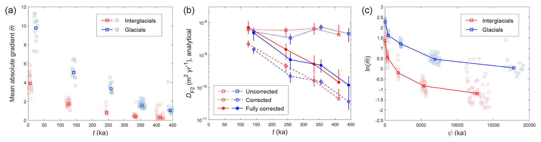
Figure 7 Inversion of effective diffusivity D_F2 from mean absolute gradient $\overline{m}$ of signals in interglacial and glacial maximum periods. (a) $\overline{m}$ of multiple ice stretches in each period, plotted against age; data from Fudge et al. (2024). Square plots the median $\overline{m}$ of each period. (b) D_F2 values computed from the mean absolute gradient data with Eq. (26) (“uncorrected”), with Eq. (29) (“corrected”, i.e., D_E values), and with Eq. (29) and a further multiplication by 2.5–4 times (“fully-corrected”; the multiplicative range extends the uncertainty around each value). All of these inversions study the intervals between successive interglacials (red) and between successive glacial maxima (blue), as in Fig. 6c. Symbols plot median values, and vertical bars plot interquartile ranges; the lower quartile is missing if it is negative and cannot be shown on log scale. (c) ln($\overline{m}$) against the AICC2012-based dilated age ψ for the periods studied. The squares plot median values.

Recall that D_F2 is the uncorrected effective diffusivity, equivalent to F2024's estimate, and D_E corrects D_F2 for misamplification by the factor (${\mathit{\psi }}_{\mathrm{2}}-{\mathit{\psi }}_{\mathrm{1}})/(t_{\mathrm{2}}-t_{\mathrm{1}}$), which is larger the older is the interval (Sect. 2.3). Indeed, the inversion results in Fig. 7b show that whereas the median D_F2 values (≈ 3.3–7.2 × 10⁻⁹ m² yr⁻¹; squares) are broadly level and consistent with the D_F2 estimates of F2024 (4.8–6.1 × 10⁻⁹ m² yr⁻¹; see their Table 1), the median D_E values (open circles) decrease with age and are much lower than D_F2. The difference attests a strong overestimation in D_F2, even for the shallowest results at 125 and 142 ka.

We further correct D_E for the issue with k^* in the Barnes et al. (2003) method by multiplying them by 2.5–4 (Sect. 2.3). This yields the “fully-corrected” D_F2 estimates in Fig. 7b (filled circles). This correction returns the shallowest results roughly to the uncorrected D_F2 medians. But the strong decreasing trend remains: the deepest fully-corrected estimates at ≈ 400 ka are nearly 2 orders of magnitude less than the shallowest values. The uncertainties in Fig. 7b are relatively small, so the trend cements the finding from D_F1 (Sect. 3.2) that the true diffusivity decreases with age.

This decrease in D is confirmed separately by the exact inversion $D=-(\mathrm{1}/k^{*\mathrm{2}})\mathrm{d}\left(\ln \overline{m}\right)/\mathrm{d}\mathit{\psi }$ in Eq. (28). Figure 7c plots ln($\overline{m}$) against dilated age ψ, showing a reduction of the slope of the plot trajectories – and thus D – with age. For both interglacials and glacial maxima, the slopes of the segments linking the plot points essentially give the fully-corrected D_F2 estimates of Fig. 7b. Since a smooth curve through the points won't deviate much from the segments, D(t) is well approximated by these estimates (more precisely, D will be somewhat less than these estimates, as the local slope of the curve through each point would be shallower than the segment leading left from it). Consequently, the fully-corrected D_F2 results in Fig. 7b approximately describe how the true diffusivity varies from ≈ 100 to 400 ka. These results, except perhaps the shallowest interglacial result, should be free from bias by the high, steeply decreasing D in the shallow subsurface inferred in Sect. 3.1.

The deepest values of $\overline{m}$ that we use from F2024 (between 400 and 450 ka, Fig. 7a) might include signal variability from the anomalous trough-sided peaks at depths ≳2700 m (Sect. 1). If so, our deepest two fully-corrected D_F2 values in Fig. 7b would be underestimated, but this does not affect the decreasing trend in 100–360 ka. Also, any underestimation is probably limited because F2024 found an unusual increase in $\overline{m}$ only in ice older than 550 ka (their Fig. 6). Our D_F1 results (Sect. 3.2) may be also corrupted by the anomalous peaks, but, as noted next, will not be used in our final inversion.

Figure 8 Forward modelling of the effective diffusivity profile D_R(t) from the true diffusivity profile D(t), and least-squares fitting to constrain D(t). As described in Sect. 3.4, panels (a) and (c) report an experiment assuming a flat floor for D; and panels (b) and (d), an inclined floor. (a, b) Plot of log diffusivity versus age, showing D(t) (dashed), the predicted D_R(t) profile (solid curve), and D_R data from peak-amplitude inversion (points). Panel (b) includes the fully-corrected D_F2 results of Fig. 7b for comparison. Grey shading about D(t) shows its maximal variation as found from the confidence intervals of the best-fit parameters, t_c and D_c. (c, d) Root mean square (RMS) mismatch in log-10 scale between predicted and estimated D_R values, as a function of the corner age t_c and corner diffusivity D_c of the D(t) profile. White crosses locate the optimal t_c and D_c values in (a) and (b), which yield RMS mismatches of 7.16 and 6.70, respectively.

3.4 Forward modelling to estimate D(t)

So far, we learned that the true diffusivity D drops steeply in the first few ka from ≈ 10⁻⁶ m² yr⁻¹ by at least an order of magnitude (Fig. 5h; Sect. 3.1) and decays further from ≈ 100–450 ka, roughly following the fully-corrected median D_F2 estimates (Fig. 7b; Sect. 3.3). What profile of D(t) with these characteristics best explains the effective diffusivity estimates D_R and D_F2 (after full correction)? Can it explain these simultaneously, and thus reconcile R2024's and F2024's findings?

To study this, we use Eq. (19) to predict the D_R(t) profile from D(t), posing the following form for D(t) on the semi-logarithmic plot. Starting from 10⁻⁶ m² yr⁻¹ at t=0, it decreases linearly to a corner value D_c, at age t_c, followed by either a flat floor (D=D_c) or an inclined floor for t>t_c. The inclined floor is assumed to have a slope equal to the mean slope of the fully-corrected median D_F2 estimates (Fig. 7b), but its level is fixed by the corner location, not by the estimates. For either floor type, we find the combination of D_c and t_c that best-fits the predicted D_R(t) profile to our AICC2012-based D_R estimates (Fig. 4b, magenta points). The D_F1 results (Fig. 6c) are excluded from the exercise, given their large uncertainties.

Figure 8 shows the best-fit profiles and maps of misfit over the t_c–D_c parameter space from the forward modelling. In the flat-floor experiment (Fig. 8a, c), the predicted D_R(t) profile fits the D_R estimates moderately well, and D decreases from its surface value to the corner diffusivity D_c≈2.1 × 10⁻⁹ m² yr⁻¹ in 9.1 ka. In the inclined-floor experiment (Fig. 8b, d), D_R(t) fits the D_R estimates better, capturing their gentle decay trend at large t. Here, D(t) has a shorter initial drop (2.8 ka), D_c is higher (≈ 1.74 × 10⁻⁸ m² yr⁻¹), and the floor shoots through the fully-corrected D_F2 values even though their level is not a fitting target; D(t) also lies slightly below their trend, as anticipated. Thus, this D(t) profile (Fig. 8b) explains the mean absolute gradient data as well as the peak-amplitude data and yields the better reconstruction of the two experiments. It also gives a more plausible estimate of the true diffusivity than the opposite conversion from D_R to D (Sect. 3.1), which reconstructed negative D intervals. Its steep initial drop is mainly constrained by the D_R decay in 0–50 ka, and its inclined-floor level by the deeper D_R values. Importantly, the corner age (2.8 ka) confirms our finding from Sect. 3.1 that the high D decaying through the upper column does not extend far below the firn-ice transition. Note that D(t) in Fig. 8b is reliable to a maximum age of only ≈ 390 ka (≈ 2700 m) because the deepest D_R and fully-corrected D_F2 data constraining the fit are interval-based results.

In these experiments, the long tails on D_R caused by the high initial D values confirm the memory effect, and the D(t) profiles are broadly consistent with the Holocene D_eff estimate of Barnes et al. (2003), ≈ 1.3 ± 0.6 × 10⁻⁷ m² yr⁻¹ after applying the k^*-correction (Sect. 2.3). That D(t) in Fig. 8b lies below the D_R, D_F1 and D_F2 estimates of R2024 and F2024 by up to 1–2 orders of magnitude confirms that these effective diffusivities approximate D crudely, and that the discrepancy between them stems from the underlying averaging, the different intervals used to evaluate them, and errors in the mean absolute gradient method.

Finally, the D_R estimates being fitted depend on the assumed 3-year FWTM duration for the surface peaks (Sect. 2.1). To gauge the impact of this assumption, we conducted an ensemble of 10⁵ best-fit forward model runs, where each of the 537 D_R estimates serving as fitting target in each run was picked randomly from its three values based on FWTMs of 1, 3, and 5 years. The maximal ranges found for t_c and D_c are 2.3–2.9 ka and 1.70–1.78 × 10⁻⁸ m² yr⁻¹, respectively, narrowly bracketing the results in Fig. 8b. This is not surprising as D_R is weakly sensitive to the FWTM, as found by R2024.

3.5 Diffusivity inversion in the firn

The preceding inversions highlight the firn diffusivity as a key interest, but their methods ignore firn densification and assume an EDC column consisting of ice only. Might the high D found for the firn be an artefact of this neglect? Should the methods be adjusted to account for firn density change? The D_R inversion is especially relevant in this regard, as it involves signals descending through the firn layer; its results are also used in the estimation of D(t) (Sect. 3.1 and 3.4). Here we show that because of the way the bulk concentration C is defined and used, Eq. (1) correctly describes signal evolution in the firn as well as in the ice, so that the D_R inversion and our findings for D are valid.

The concerns are two-fold. R2024's reconstruction of the original surface peaks, which provides input data for the D_R inversion and takes each peak's width (FWTM) to be 3a, uses the ice-equivalent thickness and assumes surface material with the ice density ρ_i (917 kg m⁻³) throughout calculation (Sect. 2.2.1). If the firn surface density ρ₀ (< ρ_i) is used in the reconstruction, each original peak would be wider (3$a{\mathit{\rho }}_{\mathrm{i}}/{\mathit{\rho }}_{\mathrm{0}}$), its height proportionally less, so α may have been underestimated and D_R overestimated. A second concern is that Eq. (1) might not conserve the amount of impurity in densifying firn. With D defined as the diffusivity of the bulk material (ice–air composite in the case of firn), $D{\partial }^{\mathrm{2}}C/\partial z^{\mathrm{2}}$ in Eq. (1) describes impurity flux divergence only if C is the impurity amount per unit volume of bulk material, not if C is impurity amount per unit mass – as used by us and R2024 in the D_R inversions. Consequently, one fears that Eq. (1) might be the wrong model, and it is unclear whether D presently retrieved for the firn describes its bulk diffusivity or some other quantity.

We dispel these concerns in the following by deriving Eq. (1) from first principles. Consider the firn layer in the Cartesian coordinates (X, Y, Z), with depth Z measuring down from the surface. Let U = (U, V, W) be the firn velocity, and ρ=ρ(Z) be the firn density profile, assumed time-invariant. We define the bulk concentration c_B as the impurity amount per volume, i.e., c_B=ρC. Then, impurity conservation obeys

$$\begin{array}{}\text{(32)}& {\displaystyle \frac{\partial c_{\mathrm{B}}}{\partial t}}+\mathbf{\nabla }.\left(\mathit{U}{c}_{\mathrm{B}}\right)=\mathbf{\nabla }.\left(D\mathbf{\nabla }{c}_{\mathrm{B}}\right),\end{array}$$

in which D=D(Z) describes the vertical diffusivity profile, and the equation for water mass conservation is

$$\begin{array}{}\text{(33)}& {\displaystyle \frac{\partial \mathit{\rho }}{\partial t}}+\mathbf{\nabla }.\left(\mathit{\rho }\mathit{U}\right)=\mathrm{0}.\end{array}$$

At ice-sheet divide or summit locations, ρ, c_B and W have negligible horizontal variations (they are functions of Z only) so the above equations become

$$\begin{array}{}\text{(34)}& {\displaystyle \frac{\partial \mathit{\rho }}{\partial t}}+W{\displaystyle \frac{\partial \mathit{\rho }}{\partial Z}}+\mathit{\rho }\mathbf{\nabla }.\mathit{U}=\mathrm{0},\text{(35)}& {\displaystyle \frac{\partial c_{\mathrm{B}}}{\partial t}}+W{\displaystyle \frac{\partial c_{\mathrm{B}}}{\partial Z}}+c_{\mathrm{B}}\mathbf{\nabla }.\mathit{U}={\displaystyle \frac{\partial }{\partial Z}}\left(D{\displaystyle \frac{\partial c_{\mathrm{B}}}{\partial Z}}\right),\end{array}$$

where W=W(Z) is the submergence velocity profile in the column.

Now suppose the depth–age scale Z=g(t), with the function g given by

$$\begin{array}{}\text{(36)}& t=g^{-\mathrm{1}}\left(Z\right)=\underset{\mathrm{0}}{\overset{Z}{\int }}{\displaystyle \frac{\mathrm{d}\mathit{\eta }}{W\left(\mathit{\eta }\right)}}.\end{array}$$

We define $z=Z-g\left(t\right)$ in order to use the reference frame of Eq. (1), which follows the material as it descends. The variable change from Z to z gives $\partial /\partial Z\to \partial /\partial z$ and $\partial /\partial t\to \partial /\partial t-W\left(g\right(t\left)\right)\partial /\partial z$, and Eqs. (34) and (35) become

$$\begin{array}{}\text{(37)}& {\displaystyle \frac{\partial \mathit{\rho }}{\partial t}}+\stackrel{\mathrm{̃}}{w}{\displaystyle \frac{\partial \mathit{\rho }}{\partial z}}+\mathit{\rho }\left({\displaystyle \frac{\partial U}{\partial X}}+{\displaystyle \frac{\partial V}{\partial Y}}+{\displaystyle \frac{\partial W}{\partial z}}\right)=\mathrm{0},\text{(38)}& {\displaystyle }\begin{array}{rl}& {\displaystyle \frac{\partial c_{\mathrm{B}}}{\partial t}}+\stackrel{\mathrm{̃}}{w}{\displaystyle \frac{\partial c_{\mathrm{B}}}{\partial z}}+c_{\mathrm{B}}\left({\displaystyle \frac{\partial U}{\partial X}}+{\displaystyle \frac{\partial V}{\partial Y}}+{\displaystyle \frac{\partial W}{\partial z}}\right)\\ & ={\displaystyle \frac{\partial }{\partial z}}\left(D{\displaystyle \frac{\partial c_{\mathrm{B}}}{\partial z}}\right).\end{array}\end{array}$$

In this reference frame, material seen from the horizon with age t has the velocity

$$\begin{array}{}\text{(39)}& \stackrel{\mathrm{̃}}{w}(z,t)=W\left(g\right(t)+z)-W\left(g\right(t\left)\right).\end{array}$$

On the short length scale of the signals (∼ 10⁻¹–10⁰ m), the vertical gradient of velocity W can be approximated by the strain rate, so $\stackrel{\mathrm{̃}}{w}\approx {\dot{\mathit{\epsilon }}}_z\left(t\right)z$. Density and diffusivity variations across individual signals can be assumed to be small on this scale, so we take $\partial \mathit{\rho }/\partial z\approx \mathrm{0}$ and $\partial (D\partial c_{\mathrm{B}}/\partial z)/\partial z\approx D{\partial }^{\mathrm{2}}{c}_{\mathrm{B}}/\partial z^{\mathrm{2}}$. Applying the first of these approximations in Eq. (37) yields the compaction relation $\partial U/\partial X+\partial V/\partial Y+\partial W/\partial z=-(\partial \mathit{\rho }/\partial t)/\mathit{\rho }$, which, when used in Eq. (38), converts it to

$$\begin{array}{}\text{(40)}& {\displaystyle \frac{\partial c_{\mathrm{B}}}{\partial t}}-{\displaystyle \frac{c_{\mathrm{B}}}{\mathit{\rho }}}{\displaystyle \frac{\partial \mathit{\rho }}{\partial t}}=D{\displaystyle \frac{{\partial }^{\mathrm{2}}{c}_{\mathrm{B}}}{\partial z^{\mathrm{2}}}}-{\dot{\mathit{\epsilon }}}_z\left(t\right)z{\displaystyle \frac{\partial c_{\mathrm{B}}}{\partial z}}.\end{array}$$

This is an approximate general evolution model for signals on c_B in firn or ice.

In the ice, where ρ≡ρ_i (constant), Eq. (40) loses the compaction term and reduces to the same form as Eq. (1). This means that Eq. (1) is valid in the ice whether the bulk impurity concentration is defined in per mass or volume terms.

In the firn, Eq. (1) is missing the compaction term of Eq. (40) so it cannot be used to track c_B. But by substituting c_B=ρC into Eq. (40), we recover Eq. (1) exactly after some algebra. This means that Eq. (1) is valid in the firn and is the right model for formulating the diffusivity inversion, provided that C measures the bulk impurity concentration in per mass terms, as done by R2024 and us here. Inversions with the impurity concentration in per volume terms must use Eq. (40) instead.

It follows that R2024's reconstruction of the original peaks gives the right inputs, and the D_R inversion is valid for both peaks in the firn (which experienced diffusion in a densifying material) and peaks in the ice (which experienced diffusion in a densifying material and then diffusion under constant density). A further realisation unknown to the earlier studies is that D retrieved for the firn by inversions based on Eq. (1) automatically quantifies its bulk diffusivity. It thus turns out fortunate that R2024 used the chemical measurements expressed as sulphate concentration in per mass terms directly as C in Eq. (1).

4 Physical controls on sulphate diffusion at EDC

Armed with D(t) from Fig. 8b, we discuss the mechanisms of sulphate transport in the EDC column, going beyond the interpretations made by R2024 and F2024 from their effective diffusivities. D drops steeply from its surface value ≈ 10⁻⁶ to ≈ 1.7 × 10⁻⁸ m² yr⁻¹ at 2.8 ka, an age coinciding roughly with the firn base (≈ 2.5 ka at 100 m depth); this drop is much shorter in duration than the initial decay in D_R (Figs. 1c and 4). A slower decay in D to ∼ 10⁻¹⁰ m² yr⁻¹ follows from 2.8–390 ka, although its real form may not be exactly log-linear as posited in our forward model; D is similar at ≈ 125 ka to the D_F1 and D_F2 estimates of F2024 (1.6–6.1 × 10⁻⁹ m² yr⁻¹) but much lower in deeper ice. We consider these intervals in turn.

4.1 Vapour diffusion in the firn

Recall that D retrieved for the firn reflects its bulk diffusivity (Sect. 3.5). We interpret the high D on the steep drop as being due to diffusion of H₂SO₄ vapour through interconnecting air pores in the firn. This mechanism is plausible because H₂SO₄, though often viewed as nearly non-volatile, does have a vapour pressure (Tsagkogeorgas et al., 2017).

A back-of-the-envelope calculation of the diffusion rate involving the H₂SO₄ vapour pressure p_v and H₂SO₄ diffusion coefficient Ω_a in firn air supports the interpretation. We assume H₂SO₄ transport by vapour diffusion to be much faster than solid-state diffusion of sulphate through ice grains, but slow compared to sulphate exchange between ice and air, such that vapour diffusion is rate limiting. This assumption, which is justified by the time scales found below, features also in the Whillans and Grootes (1985) model for water isotope diffusion in firn, except evaporation replaces fractionation of the species here. To estimate p_v, we assume sulphuric acid to be available on firn grain surfaces to exchange with vapour; then, Eq. (11) of Tsagkogeorgas et al. (2017) gives p_v ∼ 5 × 10⁻⁹ Pa at −53 °C. To estimate Ω_a, we extrapolate the H₂SO₄ diffusion coefficients measured by Brus et al. (2017) at 278–298 K under laminar conditions to ≈ −50 °C, finding Ω_a ∼ 0.015 to 0.05 cm² s⁻¹ or ∼ 45 to 150 m² yr⁻¹ when bearing in mind the uncertainty in its power-law temperature dependence noted by these authors (see their Fig. 5 and Table 1). We adopt Ω_a∼ 150 m² yr⁻¹ from the top of the range, as it is based on a weaker temperature dependence (a power of 1.5) that is more consistent with the one (1.75) found across the literature on gas diffusion (e.g., Tang et al., 2014).

Now, if we focus on the top few metres of the firn and account for the relative density ${\mathit{\rho }}_{\mathrm{0}}/{\mathit{\rho }}_{\mathrm{i}}$ ∼ 0.4 there, then the diffusion coefficient for the bulk firn would be less, ≈ ${\mathrm{\Omega }}_{\mathrm{a}}(\mathrm{1}-{\mathit{\rho }}_{\mathrm{0}}/{\mathit{\rho }}_{\mathrm{i}}$), but this correction is offset by a strong enhancement of diffusion by firn ventilation and wind pumping (e.g., Colbeck, 1989; Waddington et al., 1996). We therefore proceed by using the free-air diffusivity Ω_a without correction. A ballpark estimate of D from vapour diffusion is found by scaling Ω_a by the abundance ratio of SO${}_{\mathrm{4}}^{\mathrm{2}-}$ in the air to ice. The vapour pressure p_v converts via the ideal gas law to 2.7 × 10⁻¹² mol m⁻³, whereas for a volcanic signal in the firn with bulk concentration peaking at 200 ppb (≈ 2 nmoles g⁻¹), the peak sulphate abundance is ≈ 2 mmol m⁻³ in the ice grains or ≈ 0.8 mmol m⁻³ in the bulk firn. The resulting abundance ratio, ≈ 3 × 10⁻⁹, leads to the bulk diffusivity D ∼ 4.5 × 10⁻⁷ m² yr⁻¹, similar to the shallow high values on our D(t) profile.

The assumption regarding time scales may be checked. For signals on the decimetre scale l ∼ 0.1 m, the vapour-diffusion time scale, $l^{\mathrm{2}}/D\sim$ 10⁴ year, is much longer than the solid-diffusion time scale, $d_{\mathrm{g}}^{\mathrm{2}}/D_{\mathrm{s}}$ ∼ 400 years. These values are based on the mean grain diameter d_g in the upper firn at Dome C (≈ 0.1–0.2 mm; Gay et al., 2002) and the assumption that the H₂SO₄ diffusivity within ice grains, D_s, is similar to the H₂O self-diffusivity of monocrystalline ice (∼ 10⁻¹⁰ m² yr⁻¹ at −53 °C).

The vapour diffusion model also explains the steep drop of D in the range ≈ 0–2.8 ka, because firn metamorphism reduces the porosity and seals off interconnecting airways to lower the bulk diffusivity (Calonne et al., 2022) on descent through the firn layer, and because as grain growth occurs in the firn, larger grains slow the H₂SO₄ diffusion from their interior to their surfaces, progressively limiting the bulk diffusion rate. At pore close-off (ρ≈845 kg m⁻³ at Dome C; Calonne et al., 2022) vapour diffusion terminates, and other processes must control D thereafter.

4.2 Sulphate transport below the firn-ice transition

Below pore close-off at EDC, signal smoothing may result from (i) solid-state diffusion within ice grains, (ii) “Gibbs–Thomson diffusion” of vein signals (Ng, 2021; i.e., diffusion of the part of sulphate bulk concentration in liquid veins due to thermodynamic interactions including the Gibbs–Thomson effect and melting-point depression by dissolved ions), (iii) diffusion through the grain-boundary network, (iv) “residual diffusion” caused by the stochastic three-dimensional motion of veins and grain boundaries carrying impurities (Ng, 2021), and any combination of these processes. We expect suppression of Gibbs–Thomson diffusion where the veins are disconnected or blocked by microparticles or dust (Ng, 2021), and suppression of residual diffusion where such particles impede grain-boundary motion (Durand et al., 2006).

In terms of how sulphate is partitioned in EDC ice across crystal lattice, grain boundaries and liquid veins, direct observations are limited to a small number of shallow ice samples, but they indicate its presence at grain boundaries and triple junctions. Barnes and Wolff (2004) analysed 6 samples in the 140–501 m depth range with scanning electron microscopy, finding sulphur at grain-boundary sites, and at triple junctions only in samples with high sulphate concentration; they suggested that the veins could carry much impurity only when the grain boundaries were saturated. Recently, Bohleber et al. (2025) used laser ablation inductively coupled plasma mass spectrometry (LA-ICP-MS) to map the abundances of S, Cl and Na at tens-of-microns resolution in samples from 281.6, 585.2 and 1000 m depth (9, 27.3, 64 ka), in places away from volcanic spikes. Their elemental maps show strong localisation of S at grain boundaries, with little of it in grain interiors, and no apparent trend in the partitioning with depth. They argued diffusion through grain boundaries (as well as veins) as potentially playing a key role in signal evolution. Measurements targeting triple junctions with a laser spot size of 1 µm also revealed S there, but the ablated material volumes were too small for determining whether S was concentrated at the junctions – as was found for Na and Cl – and its abundance ratio between triple junctions and grain boundaries.

If D_s, D_vn, D_bn and D_res symbolise the respective “component diffusivities” contributing to D from processes (i) to (iv) above, then one might regard D as their signal-partitioning weighted sum. In the following, we assess how they conspire with signal partitioning to different impurity sites to govern D(t) in $\mathrm{2.5}\le t\le \mathrm{390}$ ka, by estimating their profiles down column. For reasons given below, we evaluate D_bn only qualitatively.

We calculate D_s, D_vn and D_res by using published equations (Appendix C) and temperature and grain-size data from EDC as input (Fig. S1 in the Supplement). These diffusivities increase with temperature. The Gibbs–Thomson diffusivity D_vn decreases with the mean grain size and sulphate bulk concentration c_B (Eq. C2). We calculate it for c_B from 1 µM (the typical background concentration at EDC) to 10 µM (order of magnitude of large volcanic peaks), noting that this range constrains a lower-bound D_vn because not all of c_B may reside in veins. For finding D_s and D_vn, empirical estimates of the molecular diffusivities of sulphate in ice single crystals and water are desired but lacking; we approximate them by the H₂O self-diffusivities in those materials.

Turning to the grain-boundary network diffusivity D_bn, we note that grain boundaries, each bounded by triple junctions, must form a discontinuous transport network that is interrupted repeatedly by triple junctions, where we envisage liquid veins to exist. Sulphate can diffuse within each grain boundary according to its molecular diffusivity, D_gb; this is probably several orders of magnitude larger than the solid-state/lattice diffusivity, D_s (Lu et al., 2009; Ng, 2024). But on the centimetre or longer scale of signals of interest (over multiple grains), the veins intersect and strongly short-circuit the grain-boundary transport; the vein-water molecular diffusivity is several orders of magnitude above D_gb (Lu et al., 2009; Ng, 2024). Consequently, grain-boundary signal diffusion is inherently coupled to vein-signal diffusion. With D_bn representing diffusion of only the part of the bulk signal in grain boundaries, we expect D_bn<D_vn because signal evolution involves sulphate diffusing along them (to and from the veins) in series with the vein short-circuiting.² Any impurity segregation where grain boundaries meet vein apices might further limit D_bn. In this way, grain boundaries are slow (diffusive) extensions of the veins. Both the coupling and segregation are poorly understood so a precise estimation of D_bn is presently out of reach.

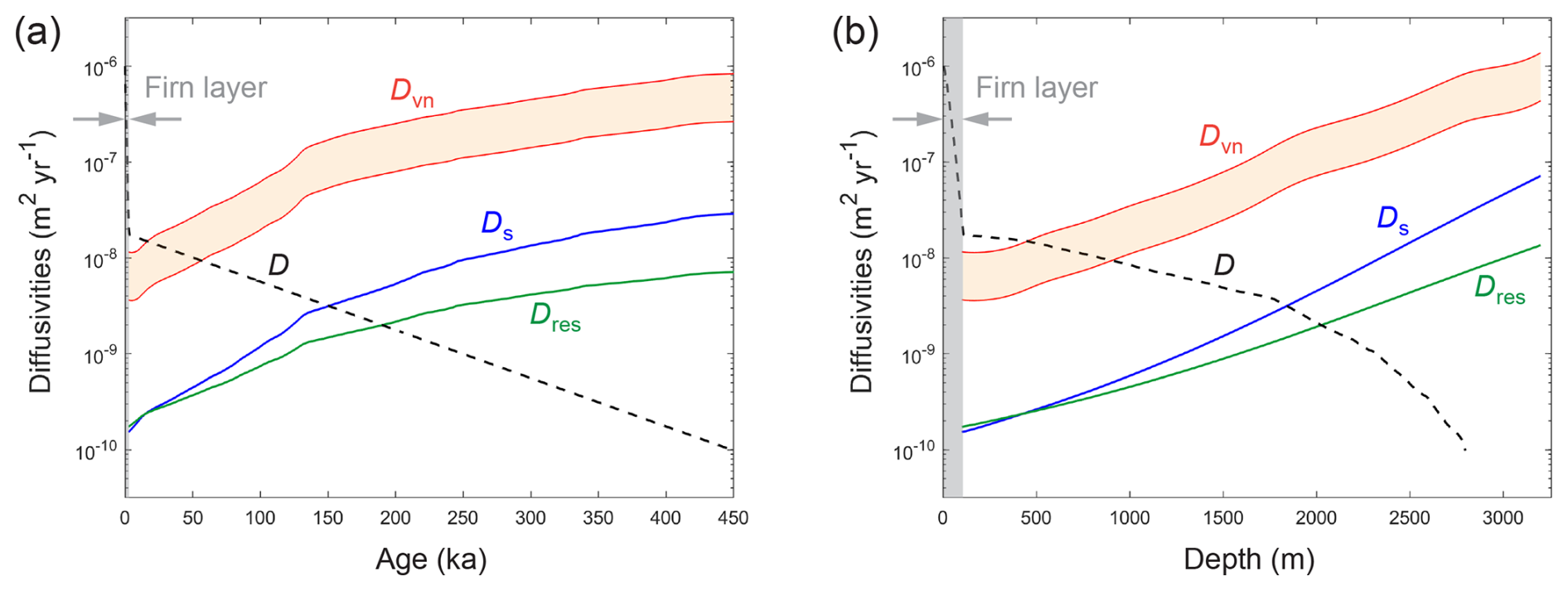
Figure 9 Estimated contributions to the sulphate signal diffusivity D in the EDC ice column (below the firn) from Gibbs–Thomson diffusion in the vein network (D_vn), solid-state diffusion within ice crystals (D_s), and residual diffusion (D_res), as functions of (a) age and (b) depth. Dashed curves plot our inversion result for D from Fig. 8b. Red shading indicates the range in D_vn described in the text.

Figure 9 shows the computed profiles of D_s, D_vn, and D_res, including D from Fig. 8b for comparison. D_vn is the highest component diffusivity. From pore close-off to ≈ 1700 m depth (≈ 130 ka), some sulphate diffusion must occur in a connected vein network because D_s and D_res are too small to account for D and because we expect D_bn to be much less than D_vn (possibly by one to several orders of magnitude). In the upper part of this interval, a sizeable fraction of sulphate signals must lie in veins, because the similarity of D_vn and D suggests that Gibbs–Thomson diffusion dominates signal smoothing, although grain-boundary diffusion in series with vein short-circuiting – as described earlier – may supplement transport. This interpretation tallies with our vapour diffusion model (Sect. 4.1), which envisages sulphuric acid present on firn grain surfaces. When the grains cross the firn-ice transition, some sulphate should end up at crystal junctions (grain boundaries and veins). Below the transition, grain boundaries may supply veins continually with sulphate, as grain growth reduces their area density. These ideas are broadly compatible with the microscale observations of Barnes and Wolff (2004) and Bohleber et al. (2025).

On descending the interval towards 1700 m, D_vn and D diverge (Fig. 9). Despite enhancement of D_vn by rising temperature (grain growth offsets this only partially, according to Eq. (C2)), D decreases. This decrease can be explained by a shift in signal partitioning away from veins. That is, each signal peak may be thought of generally consisting of a vein component, a grain-boundary component, and a crystal-interior component. The last component contributes minimally to signal evolution if we assume that the low abundance of sulphate within grains and its localisation at grain boundaries inferred by Bohleber et al. (2025) apply at all depths to 1000 m (depth of their deepest sample) and further below. As the vein component smooths by Gibbs–Thomson diffusion, the less it contributes to the peak form, so an increasing fraction of surviving signals comes from sulphate at grain boundaries, so D tends towards D_res and D_bn (note the focus on signals rather than concentration; the veins are not necessarily losing sulphate, and grain boundaries not necessarily gaining sulphate). That D has dropped to less than a tenth of D_vn at ≈ 1700–2100 m suggests that by then, most vein signals have been eliminated and grain-boundary network diffusion and residual diffusion dominantly control signal smoothing. The large decrease in D through ≈ 100–1700 m is consistent with the modelling results of Ng (2021; his Fig. 8) showing that Gibbs–Thomson diffusion rapidly damps vein sulphate signals in the upper EDC column if the veins are fully connected. In this “signal partitioning shift” mechanism, D_vn is unchanged from its estimated trajectory in Fig. 9 unless the veins are blocked or disconnected.

Progressive blockage of veins by dust that lowers their connectivity – and thus D_vn – may explain part, but not all, of the decrease in D through the interval, because Gibbs–Thomson diffusion will occur in a partially-connected vein network to cause signal partitioning shift. Consequently, signal partitioning shift with or without vein-blockage/disconnection can explain the decrease. According to R2024, vein blocking is not clearly evidenced by the EDC dust-flux record, which does not increase overall through the interval (their Fig. 5), but it cannot be ruled out while the precise microstructural distribution of dust in the ice is uncertain.

Our foregoing inferences revise the ones by R2024, who attributed the decay of D_R in 0–50 ka to a switch in diffusion mechanism due to changing location of sulphate in the microstructure and/or changing connectivity of the grain interfacial network (factors related to those identified by us above) and who interpreted the high D_R values on the decay for active diffusion through interconnected veins in ice dating to the Holocene and reaching into the last glacial. The D(t) decay analysed by us has much lower diffusivities than D_R (Fig. 8b) and extends to ≈ 130 ka, implying vein-network connectivity to greater depths. Our interpretation emphasises changing partitioning of signals (depth variations in concentration) over changing partitioning of bulk concentration (sulphate location). We also showed in Sect. 3 that the D_R decay originates from memory of very fast diffusion in the firn lasting only a few kiloyears, rather than from processes beneath the firn-ice transition.

In the ≈ 2100–2700 m interval, D continues to plunge below D_s and D_res. A plausible interpretation of this focusses on grain-boundary signals, as there is no obvious mechanism of lowering D_s substantially, and our earlier inference suggests limited vein signals surviving to these depths. The observed D may result from suppressed residual diffusion due to dust-particle drag on grain boundaries, together with grain-boundary network diffusion rates D_bn not exceeding ∼ 10⁻¹⁰–10⁻⁹ m² yr⁻¹. As D_bn≪D_s then, this interpretation suggests potential bottlenecks (e.g., segregation effects) where grain boundaries connect with veins. We emphasise that our analysis for this interval does not address the deep anomalous sulphate peaks described in Sect. 1.

These inferences from order-of-magnitude comparisons in Fig. 9 are preliminary, given the approximations for the molecular diffusivities, the uncertain size of D_bn, our use of simple models (Appendix C) that ignore other ionic impurities besides sulphate (which may impact D_vn) and potential anisotropy in grain-boundary motion and orientation (which may impact D_res) and that does not capture the coupled diffusion in grain boundaries and veins (as modelled by Ng (2024) for water stable isotopes), and given the assumptions made from the Bohleber et al. (2025) findings, which themselves are based on a few samples not carrying sulphate peak signals. Our most robust interpretation is the shift of sulphate signals away from veins and increasing dominance of grain boundaries in carrying them as we descend the upper half column.

5 Conclusions and outlook

In this paper, we advanced a theory of diffusivity inversion for impurity signals in ice cores and applied it to the sulphate datasets of F2024 and R2024 to estimate the diffusivity (D) profile at the EDC core site, gaining new insights on sulphate transport in the ice column there to ≈ 2700 m depth. Our framework unifies and extends the methods of F2024 and R2024 for finding the effective diffusivities (D_R, D_F1, D_F2) and reconciles their results. The effective diffusivities differ significantly from the local diffusivity D because they are nonuniform-weighted averages of D over large, finite age intervals. The “memory effect” from this averaging explains how the decay in D_R in ∼ 0–50 ka found by R2024 originates from high diffusivity in the thin (≈ 0–100 m equating to ≈ 0–2.5 ka) firn layer atop the column. By incorporating firn densification in the model, we show that D retrieved in the firn by the inversion measures the impurity diffusivity of bulk firn material. Our theory can be used on other ice cores and other chemical impurities to estimate the corresponding diffusivity profiles.

The EDC sulphate diffusivity profile (Fig. 8b) shows high, sharply decreasing D in the firn layer (≈ 0–100 m depth), followed by a gradual decline from ∼ 10⁻⁸ to ∼ 10⁻¹⁰ m² yr⁻¹ through ≈ 110–2700 m (≈ 2.8–390 ka). We propose vapour diffusion of sulphuric acid in firn air as the cause of the high firn diffusivity. By studying how the profile is controlled by the component impurity transport mechanisms (i.e., diffusion through crystal lattice, veins, and grain boundaries, and residual diffusion due to interfacial motion), we interpret the decline in D in ≈ 110–2000 m for a progressive removal of vein sulphate signals by Gibbs–Thomson diffusion, which leaves more and more of the remaining signals to grain boundaries, and the further decline in D in ≈ 2000–2700 m for slow diffusion through the grain-boundary network and potential slowing of grain-boundary motion by dust/microparticle drag. These factors can explain why D decreases with depth despite rising temperature. Our findings broadly agree with F2024 and R2024's interpretation (from their effective diffusivities) of limited vein-signal diffusion at depth, but yield more precise and reliable information about changing signal partitioning in the upper half column.

5.1 Implications

What of the fate of sulphate signals deposited on the surface of Dome C? Our diffusivity profile implies that if they survive the initial fast diffusion in the firn layer to “punch through” to its base, then afterwards they enjoy much slower diffusive smoothing and might survive into deep ice. For sulphate signals generally, not only volcanically-sourced spikes, we study this in Fig. 10 by computing the vertical variation of diffusion length σ (using Eq. (24) with our D profile) and using σ to predict the amplitude attenuation ratio for peak signals with annual, 3-year, decadal and centennial durations, i.e., peaks whose depositional widths at the surface are 1, 3, 10 and 100 times the mean annual layer thickness (≈ 53 mm after accounting for the surface firn density, taken as 400 kg m⁻³). The 3-year long signal is akin to the original surface peaks assumed in our inversion method, so its predicted attenuation trajectory resembles the trajectory of the α-data (Fig. 10a; cf. Fig. 4a).

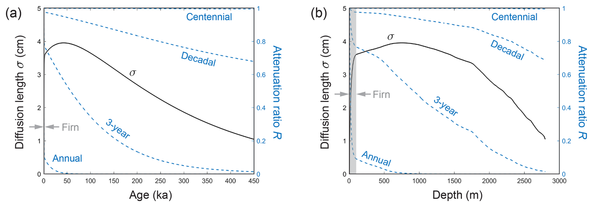
Figure 10 Diffusion length σ at the EDC core site (solid curves, left axes) against (a) age and (b) depth, calculated with Eq. (24) using the diffusivity profile D(t) from the inversion in Fig. 8b. Grey shading indicates the firn layer. Dashed curves (right axes) plot the amplitude attenuation ratio $R=\exp (-\mathrm{2}{\mathit{\pi }}^{\mathrm{2}}{\mathit{\sigma }}^{\mathrm{2}}/({\mathit{\lambda }}_{\mathrm{0}}S{)}^{\mathrm{2}}$) (equivalent to the right-hand side of Eq. (22)) for signal peaks that are annual, 3-year, decadal and centennial in duration. As these signals are not sinusoidal, we estimate R by approximating the wavelength λ₀ to be twice their widths.

As shown in Fig. 10, the initial rise in σ reflecting fast diffusion in the firn gives a total firn diffusion length of 3.6 cm. Annual signals attenuate drastically and struggle to punch through, although those with high starting amplitudes may remain detectable for some distance below the firn. Decadal and longer signals attenuate significantly less. The attenuation amount depends sensitively on the width of signals that are annual to decadal. Notably, since volcanic events vary widely in duration, their sulphate spikes in the ice have marginal survivability, in the sense that 3-year long spikes could reach ≈ 1500 m depth with $\mathrm{1}/\mathrm{3}$ of their original amplitude, but slightly shorter spikes perish much faster. This means that the FIC sulphate record presents a filtered history of volcanic forcing with short (as well as low magnitude) eruptions severely underrepresented. For non-volcanic forcings, similar low-pass filtering suppresses sub-decadal signals. Note that the sulphate diffusion lengths in Fig. 10 do not apply to water stable isotopes, and, across the depth range considered here, they are less than or similar to modelled diffusion lengths for δD in the same core (Fig. 6 of Pol et al., 2010), indicating slightly better signal preservation for sulphate compared to water isotopes.

For the ongoing Beyond EPICA – Oldest Ice (BE-OI) project and the Million Year Ice Core (MYIC) project at nearby Little Dome C, a key interest is the resolution of recoverable climate signals in ice 1–1.5 Myr old. The extreme layer thinning experienced by that ice, whose age density is expected to reach 20 kyr m⁻¹ or more at 1.5 Ma (Chung et al., 2023), will limit the retrieval and interpretation of signals of shorter than millennial time scale; e.g., centennial signals may be contained in sections ∼ 1 cm long, similar to individual grain diameter. Still, it is useful to know the diffusion length σ of (potentially observable) longer-scale signals. Here we estimate σ for sulphate in deep ice at Little Dome C, by assuming that the diffusivity profile there has the same form as found for EDC back to 450 ka and is, beyond that age, capped at 10⁻¹⁰ m² yr⁻¹, the value on our D profile at 450 ka (Fig. S2). A first calculation, made by integrating Eq. (24) again but with the thinning function S(t) derived from the modelled age–depth scales at the BE-OI and MYIC core sites (Chung et al., 2023), predicts σ=0.5–0.9 cm from 500 ka to 2 Ma (Fig. S3), with σ variations in 0–450 ka very similar to the EDC result. Separately, we then make a bounded estimate that does not depend on the age-depth scales at those sites. We use the property that the squared-diffusion lengths σ² from two contiguous parts of an ice column are additive after applying the respective vertical thinning (Gkinis et al., 2014; Ng, 2023). Thus, the value of σ² at 1.5 Ma can be found by taking σ² at 450 ka from Fig. 10 (where σ≈1 cm) and adding a σ² contribution from an extra 1.05 Myr (Δt) of signal diffusion at constant diffusivity 10⁻¹⁰ m² yr⁻¹; we deliberately ignore the effect of layer thinning on this contribution, taking it as 2DΔt, to overestimate the total σ. This second calculation conservatively constrains the maximum sulphate diffusion length to be 1.8 cm at 1.5 Ma (2 cm if made for 2 Ma).

These diffusion length results for EDC and Little Dome C (Figs. 10 and S3) pertain only to sulphate signals that entered the ice column at the top and underwent diffusion and shortening, not to signals produced or modified by other processes (e.g. the anomalous deep peaks described in Sect. 1), to which the concept of diffusion length may not apply.

Estimating the sulphate signal survival for ice-core sites outside the Dome C region is not attempted, as it requires specific knowledge about their diffusivity profiles or bolder assumptions (than for Little Dome C) to be made for those profiles.

5.2 Future research

The fast sulphate diffusion in EDC firn discovered by us, which has not been recognised before, motivates enquiry into its origin and a wider study at multiple locations. Inversions should be made with high-resolution sulphate records from other ice cores from Antarctica and Greenland to see if they show rapid firn diffusion, and to study the factors behind the diffusivity, e.g., temperature and accumulation rate. In some of those exercises, signal diffusion in the firn might not be apparent from visual inspection of the observed firn peaks (e.g., our EDC record features only 8 major sulphate peaks in the firn, amidst diverse background fluctuations, that do not show a clear trend of amplitude decay); then, as in our study, the peaks far below the firn layer may prove to be instrumental for constraining the firn diffusivity via the memory effect. Also, our proposed mechanism for the firn – involving both H₂SO₄ vapour diffusion in firn air and the assumed availability of sulphuric acid on grain surfaces (Sect. 4.1) – needs to be tested by in-situ chemical analysis in the field or laboratory experiments on firn samples. The inversion and measurement results will help us model the depth variation of D in the firn at a level of sophistication like in the Whillans and Grootes (1985) isotope diffusion model.

Another avenue concerns the grain-scale mechanisms of ionic impurity transport in polycrystalline ice, which are critical for understanding post-depositional signal alteration on ice-core records and are a known stumbling block (Stoll et al., 2021; Ng, 2021; R2024 and F2024). Although our work in Sect. 4.2 shows that we can begin to estimate the diffusivity contributions of component transport mechanisms, the partitioning of impurity to different sites and how impurity transfer between them occurs and alters the partitioning – and thus the bulk-signal diffusivity – remain poorly understood. There is also possibility for signal modification by mechanisms involving more than just diffusion, e.g., reactions between different compounds or between dissolved ions and dust particles. It is enticing to build theoretical models for all these processes, but we need abundant microscale observations of the impurity distribution to inform the effort. For sulphate, it is hoped that the LA-ICP-MS mapping of S (Bohleber et al., 2025) will soon be used to analyse much more of the length of the EDC core with dense sampling, including stretches across peak signals. The results will yield high-resolution data on dust distribution and grain size as well, which can help us understand what governs the decay on the D profile and refine our interpretation in Sect. 4.2. Accurate experimental data on the low-temperature molecular diffusivities of different ions (not limited to sulphate) in monocrystalline ice, in water and at grain boundaries are also highly desirable.

A separate challenge is to extend our inversion theory to non-steady state conditions, where the vertical profiles of D and ${\dot{\mathit{\epsilon }}}_z$ evolve with time (over glacial–interglacial time scales) as a result of climatic forcing that influences the physical properties of the ice from different periods. Such work can shed light on which of the shorter fluctuations in the effective diffusivity D_R (as discussed by R2024) reflect true diffusivity variations and how to retrieve them by inversion.

Appendix A

Table A1 Key mathematical symbols in our model.

Appendix B: Estimating the wavenumber k^*

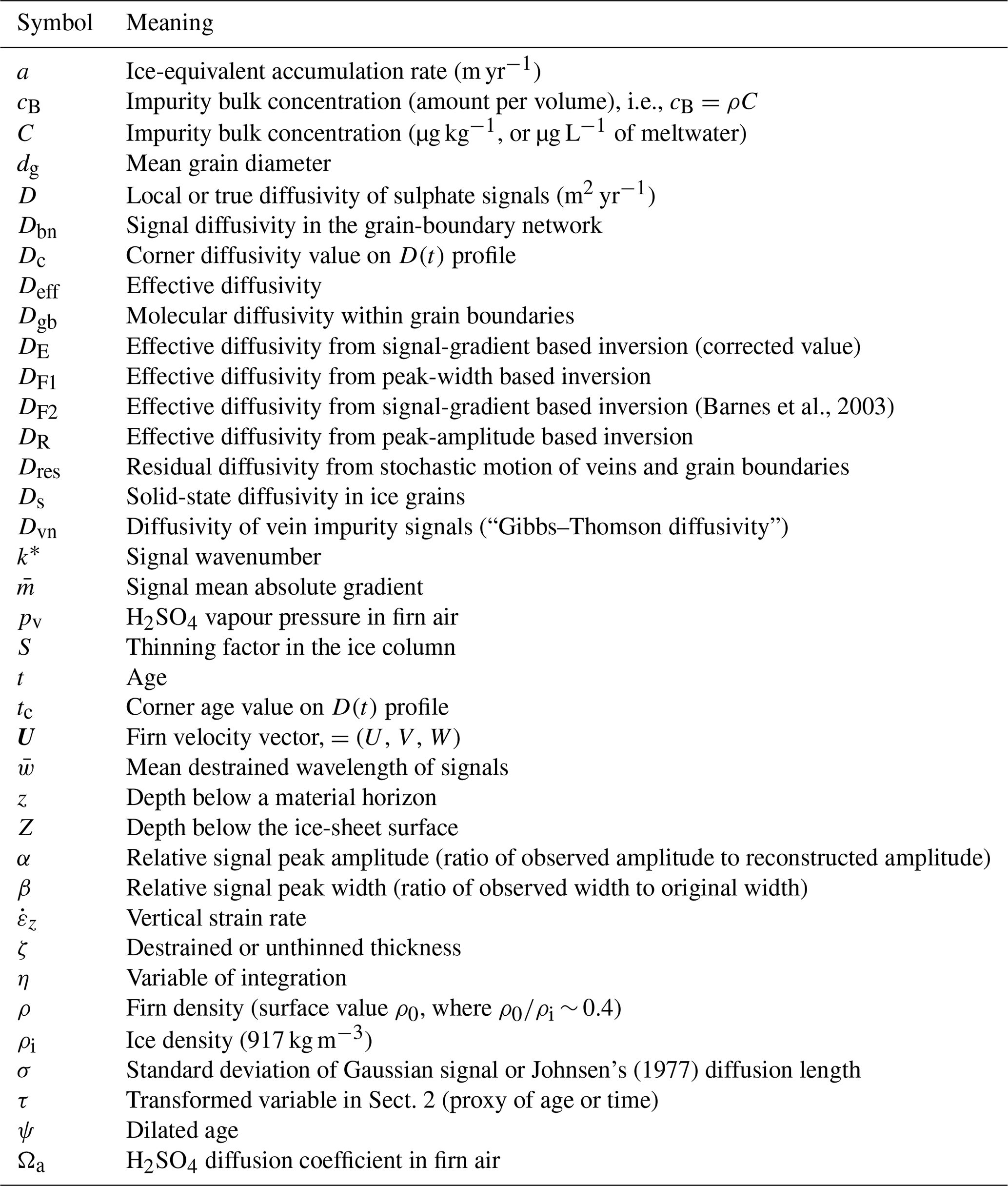
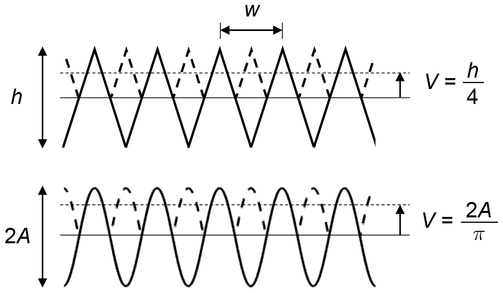
Figure B1 Test waveforms for deducing the relationship between signal height, wavenumber and mean absolute gradient.

Barnes et al.'s (2003) formula for k^* uses the mean absolute variation V of the demeaned, preprocessed and unthinned signal:

$$\begin{array}{}\text{(B1)}& V={\displaystyle \frac{\mathrm{1}}{L}}\sum _{i=\mathrm{1}}^n\left|C_{\mathrm{p},i}-{\overline{C}}_{\mathrm{p}}\right|\mathrm{\Delta }\mathit{\zeta }.\end{array}$$

For a triangular signal of height h (Fig. B1), they state the result in Eq. (31), which is equivalent to $\overline{w}=\mathrm{4}V/\overline{m}$, where $\overline{w}$ is the (mean) signal wavelength. Then they calculate the wavenumber with $k^{*}=\mathrm{2}\mathit{\pi }/\overline{w}$. In contrast, our study of this signal gives $V=h/\mathrm{4}$ and mean absolute gradient $\overline{m}=\mathrm{2}h/\overline{w}$ and hence a different result: $\overline{w}=\mathrm{8}V/\overline{m}$ – this finding holds also for an asymmetric triangular signal. A sinusoidal signal may also be considered, e.g. $A\sin (\mathrm{2}\mathit{\pi }\mathit{\zeta }/\overline{w}$) (Fig. B1). In this case, we find $V=\mathrm{2}A/\mathit{\pi }$ and $\overline{m}=(\mathrm{2}\mathit{\pi }A/\overline{w})$ mean $\left|\cos \right(\mathrm{2}\mathit{\pi }\mathit{\zeta }/\overline{w}\left)\right|=\mathrm{4}A/\overline{w}$, so $\overline{w}=\mathrm{2}\mathit{\pi }V/\overline{m}$. Consequently, Barnes et al.'s (2003) $\overline{w}$ is too small – and their k^* too large – by 2 times for a triangular signal and π/2 times for a sinusoidal signal. Real signals are typically non-periodic and different from these idealised waveforms, so k^* is overestimated by ≈ 1.57–2 times and D_eff underestimated by ≈  2.47–4 times in the Barnes et al. (2003) method.

Appendix C: Models of solid-state diffusivity D_s, vein-signal diffusivity D_vn, and residual diffusivity D_res

The sulphate diffusivity in monocrystalline ice has not been determined experimentally, as far as our literature search suggests. As described in the text, we approximate it by the H₂O self-diffusivity in monocrystalline ice and use Ramseier's (1967) empirical formula,

$$\begin{array}{}\text{(C1)}& D_{\mathrm{s}}=\mathrm{9.1}\times {\mathrm{10}}^{-\mathrm{4}}\exp \left(-{\displaystyle \frac{\mathrm{7.2}\times {\mathrm{10}}^{\mathrm{3}}}{T}}\right){\mathrm{m}}^{\mathrm{2}}{\mathrm{s}}^{-\mathrm{1}},\end{array}$$

where T is temperature in Kelvin. F2024 referred to the same approximation when qualitatively comparing their effective diffusivities to the solid-state diffusivity.

According to Eq. (23) of Ng (2021), the bulk diffusivity of ionic signals in a connected vein network in ice is given by

$$\begin{array}{}\text{(C2)}& D_{\mathrm{vn}}={\displaystyle \frac{D_l\mathit{\gamma }{T}_{\mathrm{0}}}{\mathrm{6}{\mathit{\rho }}_{\mathrm{i}}L{d}_{\mathrm{g}}}}\sqrt{{\displaystyle \frac{\mathrm{3}{\mathit{\alpha }}_{\mathrm{0}}}{c_{\mathrm{B}}\mathrm{\Gamma }(T_{\mathrm{0}}-T)}}},\end{array}$$

where D_l is the sulphate molecular diffusivity in water, c_B is the sulphate bulk concentration (by volume) in the ice, and d_g is the mean grain diameter. Equation (C2) includes a factor of $\mathrm{1}/\mathrm{3}$ to account for random orientation of the veins in three dimensions. As described in Sect. 4.2, we evaluate Eq. (C2) for c_B from 1 to 10 µM, using temperature and grain size data from EDC (Fig. S1). The following parameters from Ng (2021) are used: the reference melting point T₀=273.15 K, Gibbs–Thomson coefficient γ=0.034 kJ m⁻², latent heat of melting L=333.5 kJ kg⁻¹, vein cross-section geometrical factor α₀= 0.0725, and liquidus slope Γ=4.53 K M⁻¹ for the sulphate–H₂O system. Since empirical data for D_l below 0 °C are lacking, we approximate it with the molecular diffusivity of water by using Eq. (A1) of Ng (2023), which is valid down to −60 °C and agrees with the laboratory measurements of D_l for sulphuric acid in water from 0 to 35 °C (Umino and Newman, 1997) to within a multiplicative factor of ≈2.

Finally, for the “residual diffusivity” due to stochastic vein and grain-boundary motion, we use Eq. (9) of Ng (2021),

$$\begin{array}{}\text{(C3)}& D_{\mathrm{res}}=K_{\mathrm{0}}\exp (-Q/RT)/\mathrm{3}{c}_{\mathrm{1}},\end{array}$$

taking (as he did) c₁=2.5, the grain-growth rate coefficient K₀=1.68 × 10⁷ mm² yr⁻¹, activation energy Q=42.4 kJ mol⁻¹, and the gas constant R=8.314 J K⁻¹ mol⁻¹. Our models for the Gibbs–Thomson diffusion and residual diffusion encompass the two earlier grain-growth dependent models of ionic impurity diffusion by Barnes et al. (2003).