Contrasting patterns of change in snowline altitude across five Himalayan catchments

Seasonal snowmelt in High Mountain Asia is an important source of river discharge. Therefore, observation of the spatiotemporal variations in snow cover at catchment scales using high-resolution satellites is essential for understanding changes in water supply from headwater catchments. In this study, we adapt an algorithm to automatically detect the snowline altitude (SLA) using the Google Earth Engine platform with available high-resolution multispectral satellite archives that can be readily applied for areas of interest. Here, we applied and evaluated the tool to five glacierized watersheds across the Himalayas to quantify the changes in seasonal and annual snow cover over the past 21 years and analyze climate reanalysis data to assess the meteorological factors influencing the SLA. Our findings revealed substantial variations in the SLA among sites in terms of seasonal patterns, decadal trends, and meteorological controls. We identify positive trends in SLA in Hidden Valley (+11.9 m yr⁻¹), Langtang (+14.4 m yr⁻¹), and Rolwaling (+8.2 m yr⁻¹) in the Nepalese Himalayas but a negative trend in Satopanth (−15.6 m yr⁻¹) in the western Indian Himalayas and no significant trend in Parlung in southeastern Tibet. We suggest that the increase in SLA in Nepal was caused by warmer temperatures during the monsoon season, whereas the decrease in SLA in India was driven by increased winter snowfall and reduced monsoon snowmelt. By integrating the outcomes of these analyses, we found that long-term changes in SLA are primarily driven by shifts in the local climate, whereas seasonal variability may be influenced by geographic features in conjunction with climate.

1 Introduction

Snow is an essential water resource in High Mountain Asia (HMA), as it supplies melted water to downstream regions and regulates seasonal streamflow, especially during drought years (Pritchard, 2019; Kraaijenbrink et al., 2021). Mountain-sourced water supplies increasingly sustain human societies with drinking and irrigation water, for industrial needs, and through hydropower generation (Immerzeel et al., 2020; Viviroli et al., 2020). Snow has a cooling effect on the atmosphere by reflecting shortwave radiation and maintaining freezing ground temperatures, and a decrease in the extent of snow has been suggested as one of the causes of high-elevation warming (Palazzi et al., 2019). Therefore, understanding the current and past snow cover distribution, its ongoing changes, and its driving factors are fundamentally important.

Several studies have addressed variations in snow cover in detail for individual watersheds (e.g., Girona-Mata et al., 2019; Stigter et al., 2017), whereas large-scale assessments have predominantly focused on annual values with moderate-resolution sensors (>500 m) such as MODIS (Smith and Bookhagen, 2018; Tang et al., 2020; Kraaijenbrink et al., 2021). Past studies have used MODIS to provide a strong baseline understanding of global and regional snow phenology, including snow cover duration and extent (e.g., Johnston et al., 2023; Notarnicola, 2022; Roessler and Dietz, 2023). MODIS snow products have been essential for the constraint of snow reanalyses (Kraaijenbrink et al., 2021; Liu et al., 2021), but standard MODIS snow products may overestimate snow cover in HMA and require additional processing (Muhammad and Thapa, 2020). Furthermore, although MODIS provides daily temporal resolution and a broad perspective, the coarse spatial resolution of retrievals (500 m) poorly resolves topographic features; fractional snow cover products are a key advance but do not mitigate this problem (Painter et al., 2009; Rittger et al., 2021). Because catchment-scale snow cover derived from MODIS can be affected by cloud cover owing to spectral similarities between clouds and snow (Stillinger et al., 2019), it can be biased by high-elevation snow-free areas and struggle with shadows and subpixel effects in the extreme high-relief topography of the Himalayas (Girona-Mata et al., 2019).

The snowline altitude (SLA) is a useful metric to study snow cover variations at annual and seasonal timescales since it integrates both snowfall and snowmelt dynamics and is independent of catchment hypsometry (Girona-Mata et al., 2019; Deng et al., 2021). SLA is less biased by cloud cover than snow cover extent and is useful for evaluating and constraining hydrological models (e.g., Krajčí et al., 2014; Buri et al., 2023, 2024; Robinson et al., 2025). The seasonal pattern and aspect dependency of SLA are particularly useful to reveal the primary controls of snow cover dynamics (e.g., Girona-Mata et al., 2019). On glaciers, it can also be used as a proxy for the equilibrium line altitude (e.g., Spiess et al., 2016; Racoviteanu et al., 2019) and to constrain glacier mass balance (e.g., Mernild et al., 2013; Barandun et al., 2018). By reflecting the interplay between solid precipitation and melt, changes in seasonal snowlines can provide an important and simple indicator of climatic changes. Several previous studies have derived SLA and its changes on various scales, e.g., individual catchments to continental scales (e.g., McFadden et al., 2011; Racoviteanu et al., 2019; Girona-Mata et al., 2019; Tang et al., 2020). In High Mountain Asia, most studies have used MODIS to examine SLA changes and have highlighted a broad tendency towards shorter snow cover periods, excepting the western Himalayas, part of eastern Tibet, and part of the eastern Tien Shan (Tang et al., 2022). However, none of them have examined SLA changes and the primary controls of SLA variations at high resolution and in multiple regions to identify and understand regional differences. Analysis of seasonal variations in snow cover at high spatial resolution provides insights into snow dynamics and their relationships with climatic and geographic factors (Girona-Mata et al., 2019).

Knowledge of the regional variation in the SLA, its seasonal controls, and ongoing changes provides an important basis for a deeper understanding of current and future changes in snow cover under climate change. This study therefore aimed to answer the following research questions. (1) How does snowline seasonality vary across the Himalayas? (2) Which meteorological factors play a dominant role in controlling SLA throughout the year across this region? (3) How much and in which months has the snowline shifted in the recent 21st century? (4) Which climatic changes are associated with these changes in catchment snowline?

2 Methods

Our method to delineate snowline altitudes closely follows that of Girona-Mata et al. (2019) but is implemented in Google Earth Engine. A schematic diagram of the method is shown in Fig. 1. The framework uses an automated processing to map snow cover, masking confounding land cover types; identify boundaries of the snow-covered area; and finally retrieve topographical information corresponding to the SLA. Here we explain the approach and input datasets in more detail, before introducing our test sites and the data evaluation and analysis.

2.1 Detection of snowline altitude

Our method starts with the identification of a catchment of interest, specified by latitude and longitude. Based on these coordinates, we automatically determine the boundaries of the target catchment from the HydroBASINS version 1.0 from the HydroSHEDS database (Lehner and Grill, 2013). HydroBASINS provides 12 hierarchical levels of nested watershed boundaries according to their stream order, from which we chose level 9 for the target catchments, which is comparable in size to that used in Girona-Mata et al. (2019). To refine the domain of investigation, we used three kinds of land surface classification data: (1) glacier outlines from the latest version of the GAMDAM inventory (Nuimura et al., 2015; Sakai, 2019), (2) outlines of supraglacial debris detected by Scherler et al. (2018), and (3) maps of surface waterbodies named “Global Surface Water” created by the Joint Research Centre (Pekel et al., 2016). We used these datasets to mask these surface types as areas that may be erroneously identified as snow.

Next, the tool collects multispectral data for the target domain. We used Level-1 top-of-atmosphere (TOA) reflectance for Landsat 5/7/8 data and Level-1C TOA reflectance for Sentinel-2 data to detect snow-covered areas. The spatial resolutions of these datasets were 30 m for Landsat 5/7/8, 10 m for the visible bands of Sentinel-2, and 20 m for the shortwave infrared (SWIR) bands of Sentinel-2. We identified all scenes from to 1999–2019 period whose internal metadata indicated a cloud cover of less than 50 % of the scene.

To determine the snow-covered area, we calculated the normalized difference snow index (NDSI; Dozier, 1989), which is defined as the relative magnitude of the reflectance of the visible (green) and shortwave infrared (SWIR) bands. The NDSI approach is an established, robust, and accessible method for mapping snow in a variety of illumination and atmospheric conditions and is applicable to both TOA and surface reflectance values. There is an extensive precedent for NDSI as a practical method for identifying snow, although threshold values are not always transferable between settings (e.g., Burns and Nolin, 2014; Dozier, 1989; Gascoin et al., 2019; Härer et al., 2018). We masked clouds based on the metadata associated with each scene and then used an NDSI threshold of 0.45 to identify snow-covered areas, which is relatively conservative but performs well against independent high-resolution measurements and spectral-unmixing approaches (Girona-Mata et al., 2019). Saturation issues are common in Landsat 5/7, where the input signal exceeds the maximum measurable signal and may bias the detected snow-covered areas. Considerable sensor improvements were made with Landsat 8 and Sentinel-2 in terms of radiometric resolution (mitigating saturation problems, as well as sensor stability, and acquisition schedule, but, fortunately, snow and ice can be mapped effectively with established approaches) (Paul et al., 2016). Rittger et al. (2021) evaluated the impact of band saturation using 25 images of Landsat 7 in the Himalayas and reported that 28 % of snow-covered pixels were saturated in the visible bands. This problem was mitigated by selecting a conservative NDSI threshold (0.45) for identifying snow.

Next, we delineated the snowline from the derived snow cover map using the Canny edge detection algorithm (Canny, 1986) which produces clean edges based on filtered local high values in image gradient. However, at this point, the snowline may include misidentified areas because snow-covered areas are often obscured by clouds, shadows, scan line corrector (SLC) error stripes, or band saturation over snow. For example, the boundary of an obscured area may be misidentified as a snowline if clouds cover the actual boundary of a snow-covered area. Therefore, we removed snowlines from potentially erroneous areas such as cloud cover, deep shadows, SLC error stripes (Landsat 7), and ice and water surfaces. The last two categories (removal of surface ice and water surfaces) were not implemented in Girona-Mata et al. (2019), but the NDSI can return high values for both surfaces, even when snow is not present (i.e., frozen water or bare glacier ice), which could bias the results. As per Girona-Mata et al. (2019), we also removed very small polygons (smaller than 35 pixels) to eliminate the effects of rock outcrops which may not be relevant for meteorological patterns (i.e., oversteepened slopes that cannot hold snow).

Finally, we retrieve topographic information for each point on the snowline boundary, including elevation, slope, and aspect. As a reference digital surface elevation model (DEM), we used ALOS World 3D – 30 m (AW3D30) version 2.2, which was produced from measurements by the Panchromatic Remote-sensing Instrument for Stereo Mapping (PRISM) on board the Advanced Land Observing Satellite (ALOS). The spatial resolution of AW3D30 is approximately 30 m (1 arcsec mesh). The target accuracy of AW3D30 was set to 5 m (root mean square value) both vertically and horizontally (Takaku et al., 2018).

Finally, we calculated the median snowline altitude for (i) the entire catchment and (ii) each 45° aspect group of each catchment. This process was repeated for all available images for each study area.

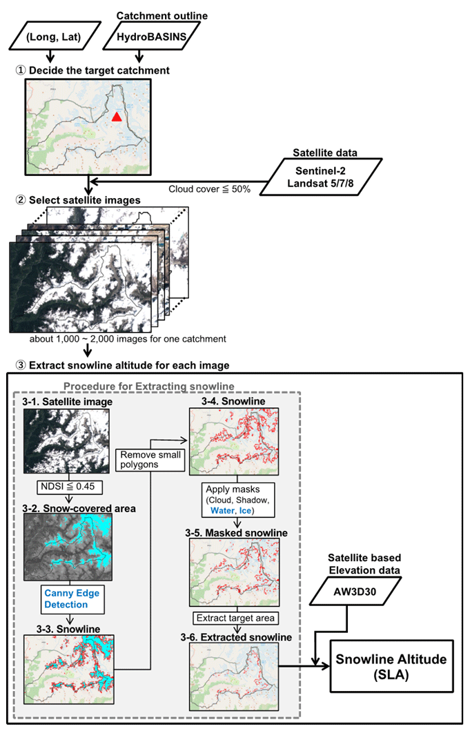
Figure 1 Schematic diagram of the snowline detection algorithm with a sample image obtained from Sentinel-2. The parts highlighted in blue represent updates to the method of Girona-Mata et al. (2019). By inputting longitude and latitude, all procedures are automatically performed on the Google Earth Engine platform.

2.2 Study sites

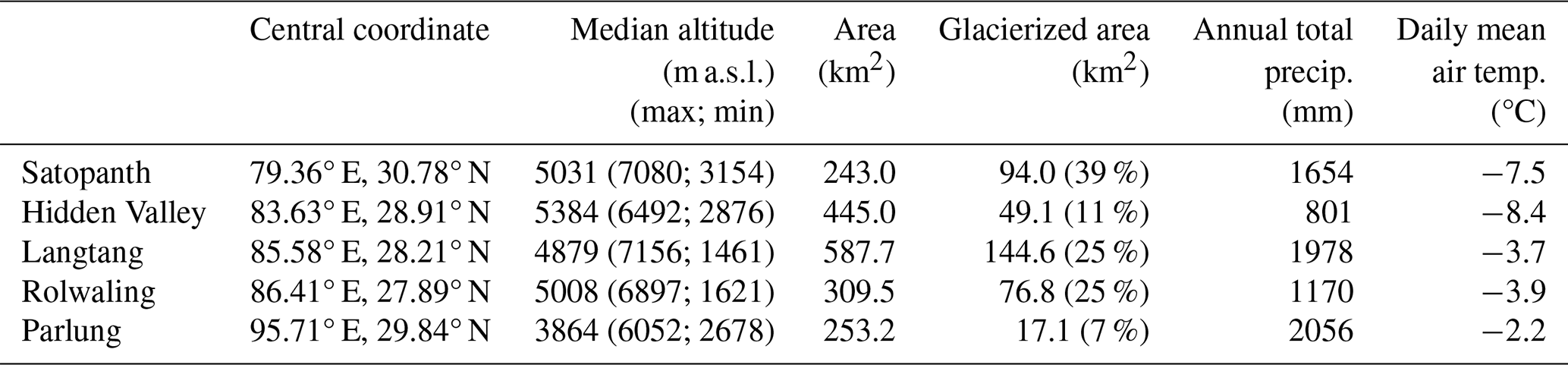
We selected five glacierized catchments along the Himalayas (Fig. 2), where hydro-glaciological studies and glacier monitoring programs have been conducted in recent years. The catchments that we identified after the representative glacier, river, or valley were, from west to east, Satopanth, Hidden Valley, Langtang, Rolwaling, and Parlung (Fig. 2). The catchments have mean elevations ranging from 3864 to 5384 m and include numerous glaciers covering 6.8 % to 38.7 % of the catchment area (Table 1). Although the Asian summer monsoon dominates the climate over its entire range, the monsoon intensity varies considerably across the five catchments. Satopanth receives limited summer precipitation and moderate winter snow from westerly disturbances (Cannon et al., 2015; Bao and You, 2019; Morinaga, 1987), whereas Parlung experiences considerable spring precipitation (Yang et al., 2013). In the other three regions, most annual precipitation occurred from June to September (Fig. S1 in the Supplement). Our scene selection criteria for these sites resulted in 6128 scenes – 1384 for Satopanth, 1173 for Hidden Valley, 967 for Langtang, 1520 for Rolwaling, and 1084 for Parlung – spread across the 1999–2019 study period (Figs. S3–S7).

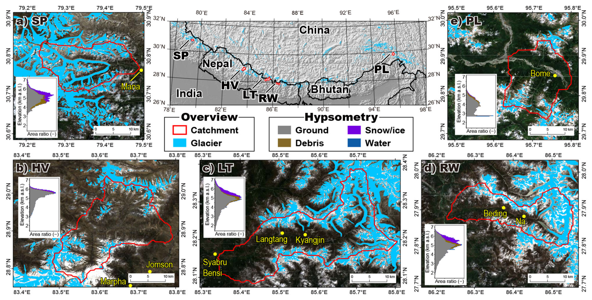
Figure 2 Upper center figure shows the location of target catchments (from west to east: Satopanth (SP), Hidden Valley (HV), Langtang (LT), Rolwaling (RW), Parlung (PL)). Enlarged views of target catchments are shown in surrounding figures: (a) Satopanth (SP), (b) Hidden Valley (HV), (c) Langtang (LT), (d) Rolwaling (RW), and (e) Parlung (PL). Catchment outlines and glaciers are indicated by red and light-blue polygons, which are sourced from the HydroSHEDS (Lehner and Grill, 2013) and GAMDAM (Sakai, 2019) databases, respectively. Yellow dots denote representative villages. The background images of (a)–(e) are composite images created using the Sentinel-2 images acquired between 2017 and 2020.

Table 1 Information on target catchments. Catchment geometric characteristics were derived from the HydroBASINS level 9 catchment boundaries and the ALOS World 3D – 30 m DEM and glacier geometries are from the Randolph Glacier Inventory 6.0, while the climatological characteristics were determined from ERA5, downscaled with an adiabatic lapse rate to the median catchment snowline elevation (see Sect. 3).

2.3 Evaluation of the automated approach

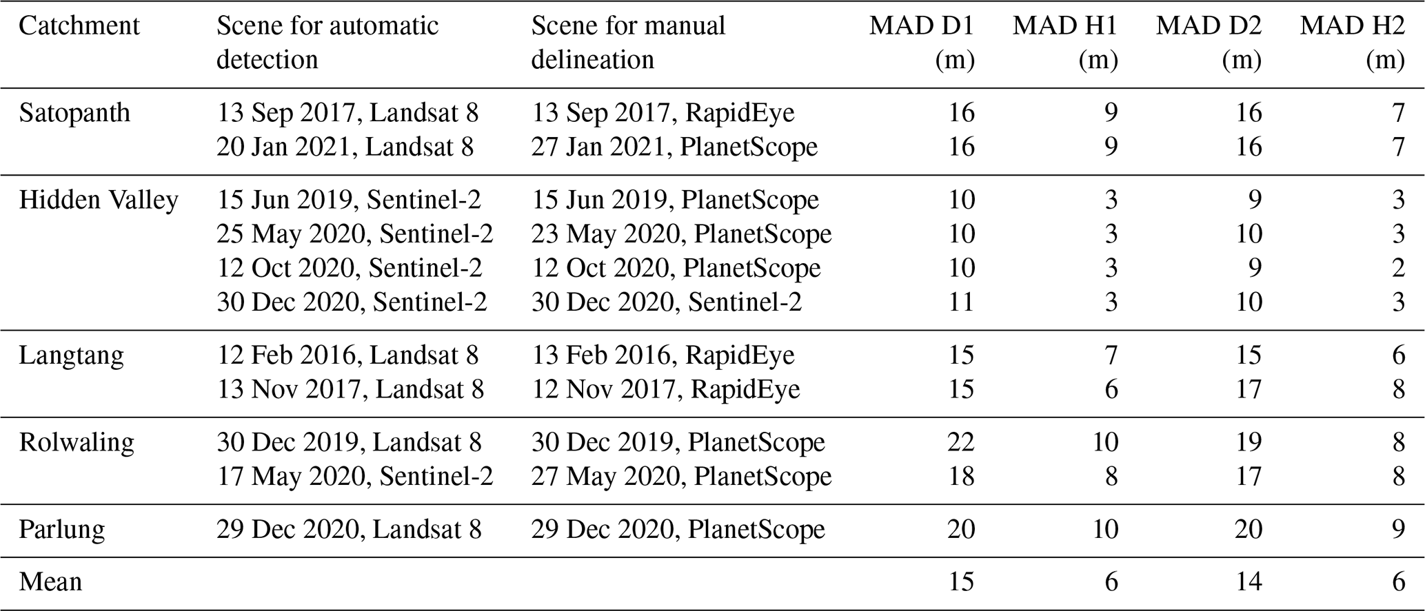
High-resolution multispectral images from RapidEye and PlanetScope were used to manually produce snowline datasets against which to evaluate the automatically detected snowlines. RapidEye and PlanetScope are both Earth observation constellations operated by Planet Labs, with spatial resolutions of 6.5 and 3.7 m. For each target catchment we prepared one to three ortho-images obtained close to the date when automatic detections were conducted from the Landsat 5/7/8 or Sentinel-2 images. A list of the images used is shown in Table 2.

The automatically detected snowlines were compared with the manually delineated snowlines obtained using high-resolution PlanetScope ortho-images obtained near the date of automatic detection (within 10 d). In manual delineations, the location of the snowline was determined by checking high-resolution satellite images as well as the glacier outline and elevation data. Because it was difficult to distinguish snowlines on ridges, we created two sets of manually delineated snowlines: (i) snowlines extracted by excluding ridges or shadows (minimum extraction, orange lines in Fig. S3) and (ii) snowlines extracted without excluding ridges (maximum extraction; blue lines in Fig. S3). We then compare each manually detected snowline point to the nearest automatically detected point in the temporally corresponding Landsat or Sentinel-2 scene and computed the horizontal and implied vertical distance (based on the DEM) between these two points. We did this for each of 12 validation scenes and for both manual slow-line delineations, producing nearly 90 000 evaluation pairs. From these, we determine the median absolute deviations of pairwise distances and height differences for each manual snowline dataset and each scene.

In addition, to investigate the agreement of SLAs derived from different satellites, we compared the SLAs derived from Landsat 7, Landsat 8, and Sentinel-2 from 2016 to 2019. Landsat 5 data were excluded from this comparison because of the operational period (March 1984 to January 2013), but we note that the predecessor approach performed favorably for Landsat 5 and 7 scenes (Girona-Mata et al., 2019). This second check is important for determining whether snowlines derived using our method from sensors with different spatial and radiometric resolutions are biased relative to one another (Rittger et al., 2021).

2.4 Analysis of SLA seasonality, trends, and controls

We first analyzed the seasonality of the SLAs by considering a dual-phase harmonic regression (Eastman et al., 2009) of the derived SLA values for the full period. The seasonal patterns of SLA in the first (1999–2009) and the second (2010–2019) half decades are compared using t tests (significance level of 0.05). For months with significant differences between the two periods, we examined the ERA5 climatic factors that could drive the SLA changes.

To examine long-term trends, satellite-derived SLA values for each scene were converted to a monthly mean. By linearly interpolating the missing values, the 21-year SLA trend was identified using the Mann–Kendall test (significance level of 0.01). We then examined the climatic factors driving SLA changes using multiple regression analysis for both annual variations (12-month moving averages) and longer-term changes (60-month moving averages).

The detected SLA was analyzed to explore the effects of orographic and meteorological controls on seasonal and long-term variations. We investigated the disparities in SLA among aspect classes (east-, south-, west-, and north-facing slopes), interpreting the observed differences conceptually using the framework proposed by Girona-Mata et al. (2019).

To further understand the seasonal and long-term controls of SLA variations, we analyzed climate reanalysis data. We obtained 0.25° gridded near-surface 2 m air temperature, downward surface shortwave radiation, cloud cover, and precipitation from ERA5 (Hersbach et al., 2020). We aggregate the hourly products into daily and monthly mean datasets. The air temperature was corrected to the average snowline altitude during the target period (1999–2019) in each catchment using a standard environmental lapse rate (0.065 °C m⁻¹). Finally, we compared the 12-month and 60-month seasonal decomposition of the SLAs with those of climatic variables (air temperature, precipitation, and solar radiation) and assessed their statistical relationships through multiple regression analysis. For this trend analysis, we use a seasonal trend decomposition based on LOESS (locally estimated scatterplot smoothing) (STL) method, which is typically a robust trend detection method for noisy data with variable sampling and strong seasonality (Cleveland et al., 1990).

3 Results

3.1 Evaluation of detected snowlines

We first present the comparison of detected SLAs from our method with those obtained through manual delineation at multiple scenes in each catchment to indicate the accuracy of the detected SLA. The SLAs obtained from our method exhibited a very close agreement with the manual delineation results (Table 2), with median absolute horizontal distances below 25 m for the nearest snowline points in all scenes and median absolute vertical distances (SLA differences) of 10 m or less. The spatial correspondence of the derived snowlines from automatic and manual methods was superb (Figs. S8–S9 for examples) for areas of overlapping coverage. Interestingly, despite this close correspondence, the cumulative distributions of snowline elevations differed substantially between the automatic and manual snowline derivations (Fig. S10), highlighting the importance of consistent catchment-wide sampling of snowline elevations. This is achievable through automated processing but not through manual delineation; we note that in situ monitoring of snowlines (e.g., Moringa et al., 1987) can thus provide rich information about temporal variability in snowlines but may be locally biased in terms of the SLA.

Considering the intersatellite variability between the SLAs retrieved from Landsat 7, Landsat 8, and Sentinel-2 (Fig. S4), we observed the least variation in SLAs during the monsoon season (with a standard deviation (σ) of SLA for all sites and satellites <18 m) and the largest variation during winter (σ<140 m). Disagreements during winter were not unexpected given the inconsistent acquisition dates for the three satellites and the variable occurrence of winter snowfall in the Himalayas. Focusing on the differences in snowline altitudes (SLAs) between different satellites during the monsoon season, we observed a high degree of consistency in the range of SLA values within each catchment. Despite heavy cloud cover, the standard deviation in the median SLA between different satellites generally remained within 50 m, except for Parlung, where the deviation extended to 120 m. Although these variations may appear significant, they are relatively minor compared to the seasonal SLA variations observed for each sensor. Therefore, we consider the bias resulting from the use of different satellites in this study to be acceptable for examining seasonal and decadal changes in the SLA.

Table 2 Performance of the automated snowline in comparison to manually digitized snowline datasets 1 and 2, reporting the median absolute deviation (MAD) for the horizontal distance (D) and vertical difference (H) of the nearest pairs of snowline points in the dataset.

3.2 Snowline seasonality

The derived SLA values demonstrate strong seasonal variability (Fig. 3). Across most sites, SLA maxima were observed during the monsoon and minima were in the winter season, which is consistent with the findings of Girona-Mata et al. (2019). However, the timing of the maximum SLA varied slightly among the sites: July in Langtang and August in Satopanth, Rolwaling, and Parlung. Hidden Valley showed a relatively stable SLA during the monsoon season, with a less pronounced maximum SLA occurring in August (Fig. 3f). The minimum SLA occurred in late winter or the early pre-monsoon season at all sites: January in Langtang, February in Hidden Valley, March in Rolwaling and Parlung, and April in Satopanth. The winter–spring SLA transition differed between sites: in Langtang SLA began to increase in January, whereas the SLA in Satopanth continued to decrease until April. All sites exhibited a relatively steady winter SLA. The differences between the minimum and maximum SLAs varied from 480 m (Hidden Valley) to 1100 m (Langtang).

All sites show strong intraseasonal dispersion in wintertime, when the range of SLA measurements is greater than the annual SLA amplitude; the winter SLA range doubles the annual amplitude in Hidden Valley, Langtang, and Rolwaling. Despite the relatively small number of images acquired during the monsoon season at all sites due to thick cloud cover, the derived SLAs for this period exhibit narrow spread and the highest SLA values. In all catchments other than Parlung, the monsoon season SLA exceeded 5500 m a.s.l.; in Parlung, the ice-free topographic availability limited snowline retrievals to 5000 m a.s.l. As noted by Girona-Mata et al. (2019), we find a strong second harmonic phase in Satopanth, Rolwaling, and Hidden Valley, which are located at high-elevation but monsoon-dominated sites. This second harmonic was less prominent in Langtang and Parlung.

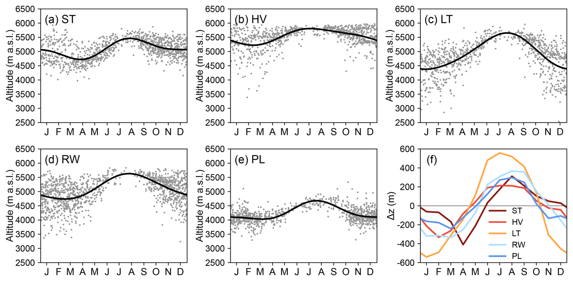
Figure 3 (a–e) The derived snowline altitude (SLA) over the target period (1999–2019) at each catchment and (f) the SLA anomaly from the mean SLA over the target period (1999–2019). Grey dots and solid lines in (a)–(e) show the SLAs derived from each satellite scene and smooth curves fitted with harmonic functions, respectively. Catchment abbreviations denote Satopanth (ST), Hidden Valley (HV), Langtang (LT), Rolwaling (RW), and Parlung (PL), respectively.

3.3 Trends in SLA for 1999–2019

The STL time series decomposition of SLAs revealed contrasting SLA trends between catchments (Fig. 4). Increasing SLA trends were found in Hidden Valley (+11.9 m yr⁻¹), Langtang (+14.4 m yr⁻¹), and Rolwaling (+8.2 m yr⁻¹), whereas Satopanth showed a decreasing trend (−15.6 m yr⁻¹) and Parlung showed no statistically significant trend (Fig. 4). These trends were confirmed for both 12-month and 60-month moving averages using the Mann–Kendall test, and the p values for the four catchments where trends were detected were all less than 0.001. The altitudinal difference between the minimum and maximum SLAs, with 12-month moving averages for each catchment, varied between 580 m (Parlung) and 820 m (Langtang).

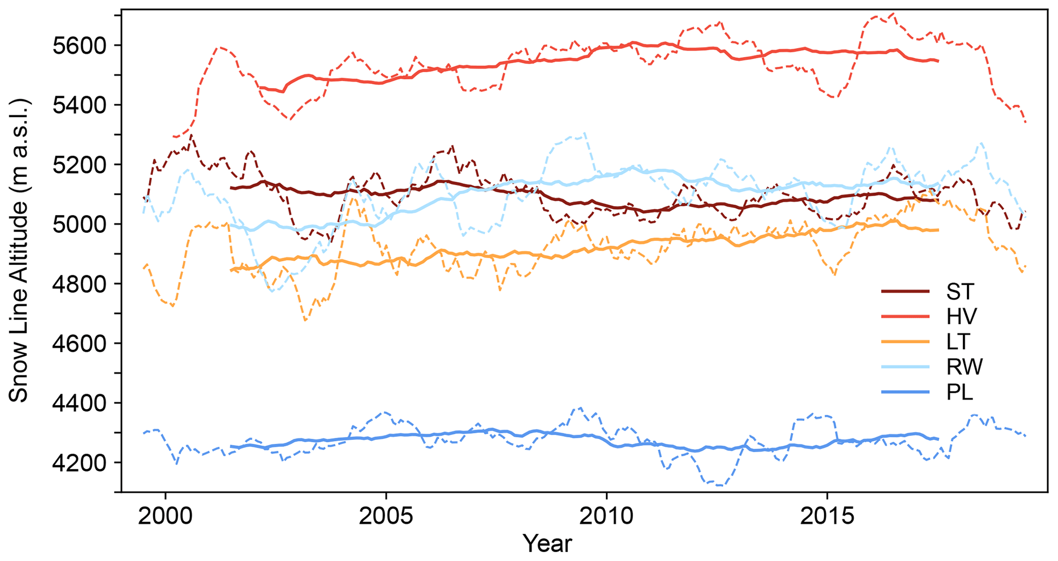
Figure 4 Snowline altitude with 60-month (solid lines) and 12-month (dashed lines) moving averages at the five target catchments. Catchment abbreviations denote Satopanth (ST), Hidden Valley (HV), Langtang (LT), Rolwaling (RW), and Parlung (PL), respectively. Trends (p<0.001) for the moving averages were −15.6 m yr⁻¹ for ST, 11.9 m yr⁻¹ for HV, 14.4 m yr⁻¹ for LT, 8.2 m yr⁻¹ for RW, and insignificant for PL.

3.4 Seasonal SLA aspect differences

Catchment snowlines showed distinct seasonal patterns of aspect dependence (Fig. 5). A common characteristic among the five catchments was the minimal difference in SLA between aspects during the monsoon season, in contrast to the substantial SLA differences between aspects during winter. Additionally, the standard deviation in the SLA, represented by the error bars in Fig. 5, was smallest during the monsoon season, gradually increasing, and largest during winter. Regarding specific regional characteristics, Satopanth showed minimal differences in the SLA between aspects, even during winter, with only a slight decrease in the north-facing SLA. Conversely, aspect-induced differences were pronounced throughout the year in the Parlung region. Furthermore, Parlung exhibited a relatively small seasonal variability in the standard deviation of the SLA values.

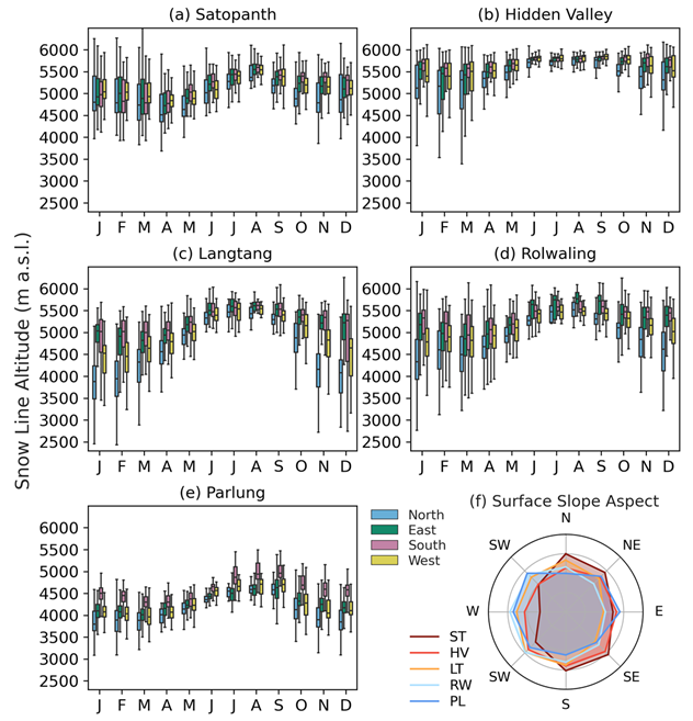
Figure 5 (a–e) Boxplots of the monthly snowline altitude (SLA) for each aspect of the slope: north, east, south, and west. (f) Relative distribution of 45° topographic aspects for each catchment (%).

3.5 Decadal changes in seasonal SLA

To examine the cause of the long-term changes in the SLA shown in Fig. 4, we compared the seasonal patterns of the SLA and climatic variables for the first half (1999–2009 in blue) and second half (2010–2019 in red) of each catchment (Fig. 6). Focusing on the months with statistically significant changes, SLA decreases were found in March in Satopanth (Fig. 6a), Hidden Valley (Fig. 6b), and Rolwaling (Fig. 6d) and in January in Parlung (Fig. 6e). No significant seasonal SLA decrease was observed in Langtang (Fig. 6c). Increases in the SLA were evident in September in Satopanth (Fig. 6a); October to December in Hidden Valley (Fig. 6b); July and October in Langtang (Fig. 6c); and July, October, and November in Rolwaling (Fig. 6d). No significant increase was observed in Parlung (Fig. 6e). Overall, SLA decreases were primarily detected in winter to early spring, with increases in the monsoon and post-monsoon seasons.

The decrease in winter SLA is associated with a decrease in temperature in January across all regions where a decrease in winter SLA was detected. The increase in precipitation during February and March may also have contributed to the lowering of winter SLAs in Satopanth, Hidden Valley, and Rolwaling. No changes in solar radiation were identifiable in relation to decreases in the winter SLA.

The rising SLAs identified in the three Nepalese catchments (Hidden Valley, Langtang, and Rolwaling) were all associated with rising temperatures during the monsoon. We note that the SLA increases occurred in conjunction with precipitation increases (all three sites) and net shortwave decreases (all except Rolwaling). Consequently, the SLA variations during the monsoon may be more closely linked to air temperature than to precipitation, shortwave radiation, or cloud cover. The decrease in solar radiation during the monsoon was statistically significant in the three Nepalese regions, which is consistent with increased precipitation. It is unrealistic for the decrease in solar radiation to contribute to the increase in SLA, but it could suppress the increasing rate of the SLA. In contrast, the increasing solar radiation in November in Rolwaling may have contributed to the increase in the SLA in the same month. In Satopanth, an increase is observed only in September, suggesting an association with the temperature increase in the same month.

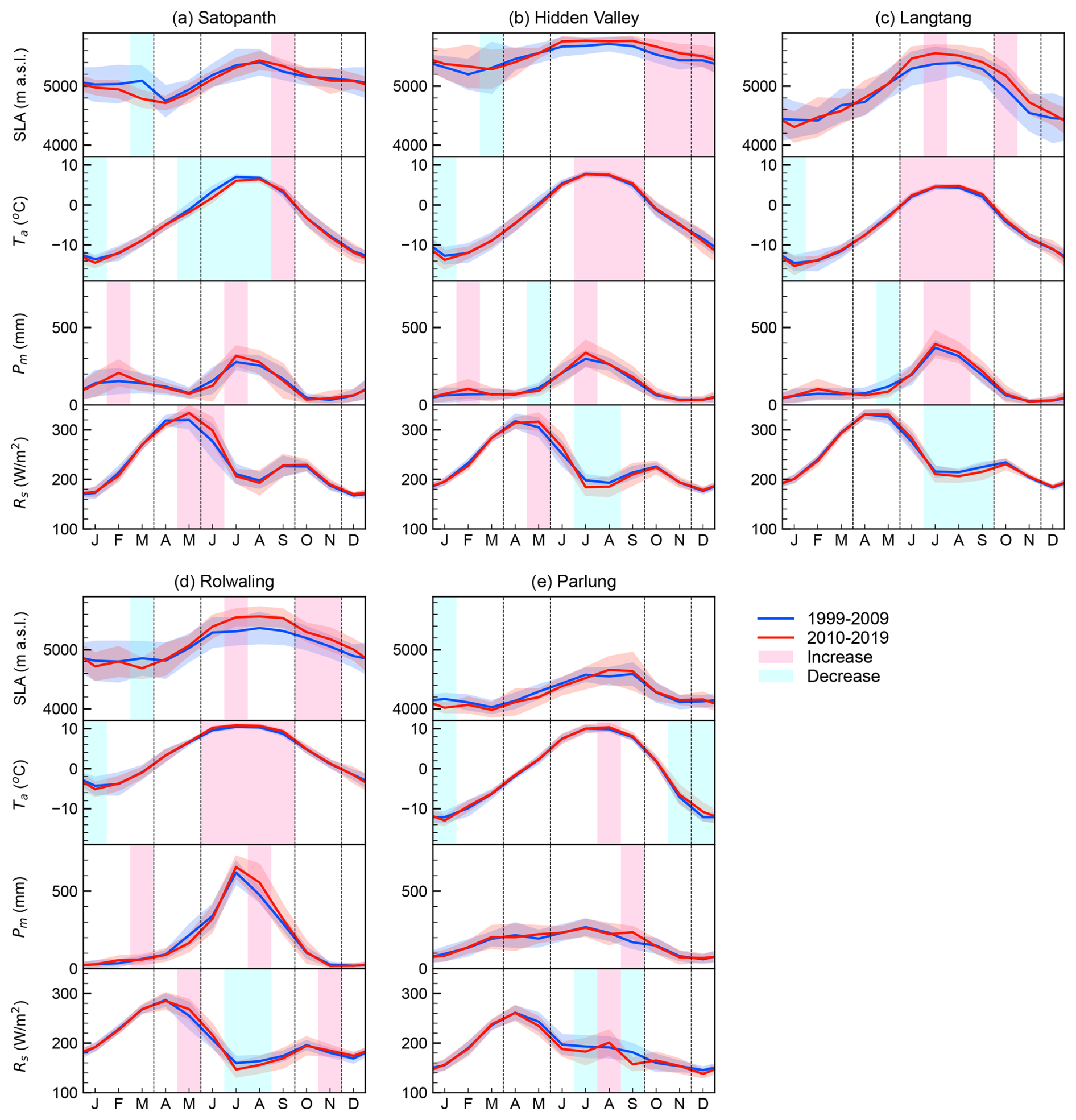
Figure 6 Monthly climatologies of SLA and climate variables (T_a, air temperature at 2 m height; Pm, monthly total precipitation; Rs, daily mean downward solar radiation flux at the surface) for the first half (1999–2009 in blue) and the second half (2010–2019 in red), respectively. Shaded areas indicate statistically significant changes (pink for increase and light blue for decrease) between the periods.

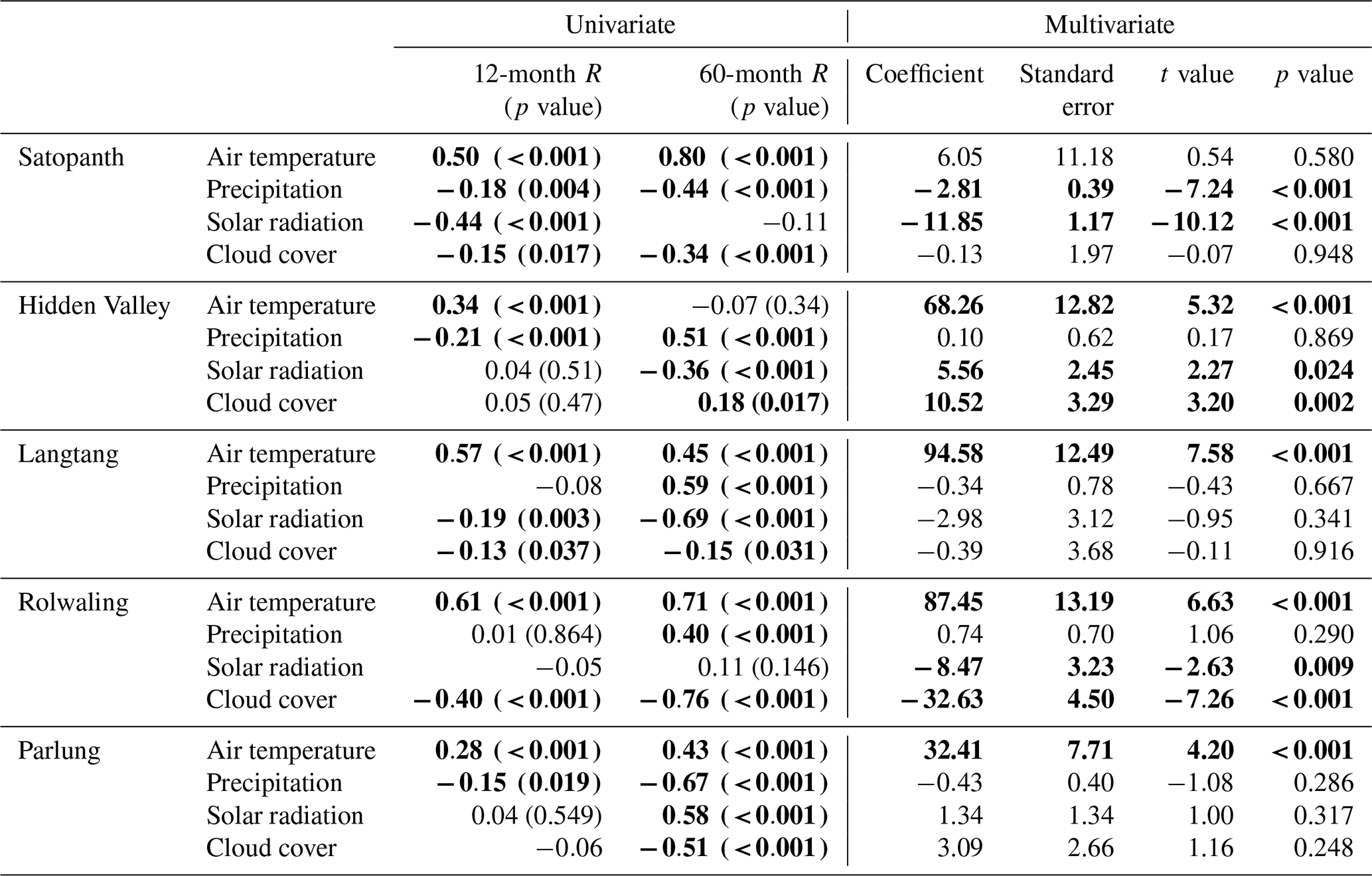
3.6 Relationships between trends in meteorology and SLA

The 12-month moving averages of snowline altitude exhibited significant correlations with changes in air temperature across most sites, except for Satopanth (Fig. 7, Table 3). In Rolwaling, all climatic variables except precipitation demonstrated a correlation with the SLA, with air temperature exhibiting the strongest impact, as evidenced by the largest t value. Conversely, in Satopanth, precipitation emerged as the sole statistical control on SLA, with a negative t value indicating that precipitation lowers the SLA. This finding that increased precipitation at the decadal scale has lowered the SLA is consistent with the results of our seasonal analyses that increased winter snowfall lowers the winter SLA in Satopanth.

Overall, our results underscore the substantial influence of air temperature on SLA variations, which is consistent with previous research (Girona-Mata et al., 2019; Tang et al., 2020). This relationship is also expected to decisively control future snow climatology in the region (Kraaijenbrink et al., 2021). However, we also found that winter precipitation can serve as a significant driving factor, particularly in Satopanth, where the SLA displays a negative trend over our study period. Although the influence of solar radiation is smaller than that of air temperature, it contributes to an increase in the SLA in Rolwaling. We also note that cloud cover plays a significant role and is negatively correlated to SLA for both Hidden Valley and Langtang.

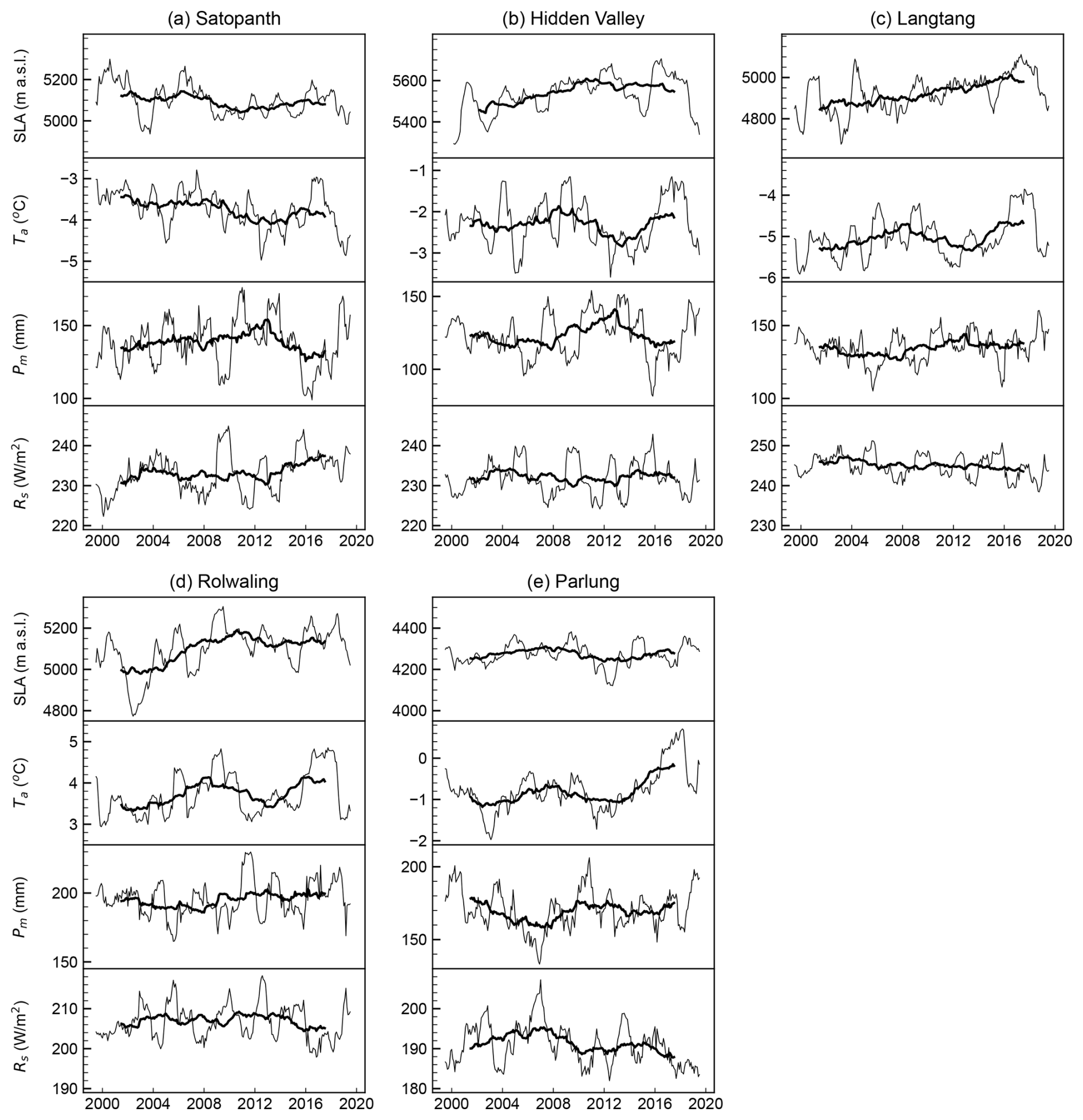
Figure 7 Time series of SLA and climate variables (T_a, air temperature at 2 m height; Pm, monthly total precipitation; Rs, daily mean downward solar radiation flux at the surface) for the period from 1999 to 2019. Variables with 60-month and 12-month moving averages are drawn with thick and thin lines, respectively.

Table 3 Correlation coefficients (R) between SLAs and single variables calculated using 12-month and 60-month moving averages and results of the multiple regression analysis using 12-month moving averages of climate data and SLA. Influential factors (p<0.05 and $\left|t\right|>\mathrm{2.0}$) are shown in bold. A positive or negative t value indicates a contribution to the increase or decrease in SLA, respectively.

4 Discussion

4.1 Seasonal pattern and controls

We found consistencies and differences in the seasonal patterns across the five target catchments. Across the five regions, the SLA reaches its highest level during the monsoon summer and is maintained at a relatively stable snow–rain transition altitude caused by abundant precipitation and altitude dependence on air temperature (Girona-Mata et al., 2019). Once the precipitation reaches a sufficient level to maintain this altitude, additional precipitation has no further impact on the SLA. Solar radiation is less effective during the monsoon summer because of frequent and heavy cloud cover, leading to highly diffused shortwave radiation (Pellicciotti et al., 2011). However, Parlung was an exception, as indicated by the minimal differences in SLA between the aspects (Fig. 5). In Parlung, differences in SLA between aspects persisted even in summer (Fig. 5), suggesting that solar radiation still has an impact on SLA.

Snow is most abundant from late winter to the early pre-monsoon season, just before the snowmelt begins in earnest. In Langtang, SLA shows the seasonal minimum in January, indicating snowmelt starting in February as solar radiation increases. In contrast, Satopanth experiences a later minimum, seeing the lowest SLA in April. This region is less influenced by solar radiation throughout the year (Fig. 5), so snowmelt may begin primarily when temperatures rise.

Winter exhibits significant variability in the snowline altitude (SLA) across catchments. Winter storms sporadically deposit snow to very low elevations, which then ablates to the seasonal freezing line, leading to increased variability in the SLA. The cumulative likelihood of these storms increases throughout the winter such that the seasonal snowline eventually converges to approximate the freezing line before the monsoon. Particularly in Langtang and Rolwaling, the variability was pronounced, with more snow cover on the west-facing slopes than on the east-facing slopes (Fig. 5). Conversely, Hidden Valley experiences less east–west variation and winter SLA variability than Langtang and Rolwaling. This could be attributed to the high-altitude Dhaulagiri mountain range to the southwest, which may act as a barrier to westerly winds, thereby limiting the inflow of moist air across the mountains. Despite being located further west, Satopanth exhibited minimal aspect variation in the SLA (Fig. 5). The Satopanth catchment features high-elevation ridges on its western side (Fig. 1).

Therefore, westerly winds (Cannon et al., 2015; Maussion et al., 2014) may have deposited more snow on the outer western slopes of the catchment area. It is conceivable that winds crossing these western ridges contributed to snowfall within the catchment. This phenomenon may explain the reduced east–west disparity observed in Satopanth compared to regions directly impacted by prevailing winds. In contrast, Parlung, located on the southeastern Tibetan Plateau, is less influenced by westerly winds. Based on the above analysis, the seasonal patterns of SLA are not only dependent on climatic factors but also are significantly influenced by topography.

4.2 Trends, decadal changes in seasonality, and controls

Long-term trends and statistically significant explanatory variables exhibited similar patterns in the study catchments (Fig. 7). Satopanth showed a declining SLA trend, primarily associated with the trend in ERA5 precipitation. In contrast, the three Nepalese catchments exhibited increasing SLA trends that were mainly associated with temperature. Parlung showed no discernible trend, with fluctuations that were possibly related to temperature variations.

We interpreted the seasonal meteorological changes driving long-term variations in SLA. In Satopanth, the declining trend was primarily driven by a decrease in SLA in March. This decrease in SLA in March could be attributed to increased snowfall in February following a temperature decrease in January. This finding is consistent with that of a previous study that reported an increasing trend of synoptic-scale western disturbance activity over the past few decades, leading to increased winter precipitation in the western Himalayas (Krishnan et al., 2019). Conversely, the rising SLA in September may have moderated the decreasing rate of the interannual trend of SLA in Satopanth. In the three Nepalese regions, the increasing trends of SLA are driven by SLA increase during the monsoon season to post-monsoon season, corresponding to rising temperatures during the monsoon season. The rising temperatures during the monsoon had a stronger effect on SLA than concurrent precipitation increases and net shortwave decrease. Although the increase in precipitation during the monsoon season is also statistically significant in these three catchments, the SLA during the monsoon may be controlled by the snow–rain transition altitude which is determined by the altitude dependence of air temperature, generalizing past inferences for Langtang by Girona-Mata et al. (2019) to the central Himalayas. It thus seems plausible that the increase in temperature is the main factor contributing to the SLA increase during the monsoon and the post-monsoon seasons.

Hidden Valley and Rolwaling also exhibited SLA lowering in March, possibly attributed to increased winter precipitation. In Parlung, a decrease in SLA due to lower temperatures was observed in January. However, this decrease in the January SLA was not sufficient to cause a long-term trend of declining SLA.

We anticipate that the long-term SLA trend is controlled by the balance between increased snowmelt during the monsoon and increased snowfall during winter. The balance between winter precipitation and summer temperature varied among the five catchments despite being located in the same Himalayan range. These results indicate that regions with different climatic and topographic characteristics, such as arid areas or those with winter accumulation, may have distinct factors controlling snow cover variability.

4.3 Reliability of trend detection

Our data-inclusive approach to snowline analyses mixes four satellite sensors with differing radiometric capabilities and sampling biases. The three Landsat sensors exhibit broad similarities in terms of spectral and temporal sampling, although with considerable improvements for Landsat 8, in particular (Paul et al., 2016). Collectively, these three sensors led to a relatively stable temporal sampling over our five study catchments, but the inclusion of Sentinel-2 data substantially increases the quantity of observations for the later period (Figs. S3–S7), in addition to the slightly different sensor characteristics. We therefore tested the effect of the Sentinel-2 data inclusion on our trend retrieval approach. The retrieved SLA trends differ for each site (up to 2.6 m yr⁻¹ difference) depending on the inclusion of Sentinel-2 data, but at no site does the trend direction or significance change based on this dataset (Figs. S14–S18).

All four sensors exhibited a similar seasonal sampling (Fig. S11), and the inclusion of Sentinel-2 data had a minimal effect on the seasonal harmonic regression of SLA (Figs. S19–S23). However, all four sensors exhibited reduced sampling during the monsoon months due to the extensive summer cloud cover, so the reliability of the trend retrieval for reduced data sampling was evaluated through a synthetic trend retrieval experiment. Beginning with a sampled harmonic and a random trend similar to that measured at our sites, we introduce noise and reduced monsoon image availability (Figs. S24–S28). Our experiment highlights that the seasonal decomposition approach is robust to both noise and seasonal sampling biases and successfully retrieves the imposed trends to within 2.5 m yr⁻¹. Our results highlight that standard regressions of oscillations around trends, even without sampling errors and biases, are subject to producing erroneous trends due to edge effects. This emphasizes the importance of long records and careful trend retrieval, such as with our seasonal decomposition approach, for environmental records with strong variability.

4.4 Limitations, advantages, and future perspectives

A major limitation for our study is the inconsistent data availability over time due to changing sensor missions, cloud cover, and the varying extent of observations. Image availability is improving due to the increased number of operational imagers but could have a strong impact on both the characterization of seasonal snow dynamics, especially for earlier periods, as well as the robust detection of a trend. A second major limitation is the prevalence of cloud cover, which further limits the usable area of affected images and can, in some cases, lead to biases in the detected snowline due to undersampling. This can be mitigated with more stringent cloud coverage criteria but will further reduce image availability for severely cloud-affected regions. Our cloud masking was largely successful for the evaluation scenes but is likely to fail in some situations, leading to false snowline detections. As detailed above, our method is able to successfully recover snowlines and snowline trends despite these challenges.

The combination of multiple datasets with differing footprints, compounded by variable cloud cover and deep shadows, can lead to sequential scenes differing in snowline, but this can be the result of spatial sampling biases. Although our evaluation of the automated snowline retrieval showed its high accuracy relative to manual datasets (Table 2), it is clear that sampling biases due to spatial coverage can lead to statistical differences at the catchment scale (Fig. S10). In our study, differences in spatial coverage may have increased the variability in derived catchment snowlines even over short timescales. Our results indicate SLA variations are typically 200 m within 10–20 d based on a variable-lag sensor cross-comparison (Fig. S28). This is reflected in the spread of seasonal retrieved SLA values (Fig. 3) but should not affect our derived trends. Nevertheless the challenge of spatial sampling underlines the importance of complete spatial coverage for integrated snowline assessments, encouraging the use of future rapid-repeat and cloud-insensitive snow monitoring methods (e.g., Tsai et al., 2019). We note that an advantage of our methodology is its transferability, and additional snow cover data products could easily be included in the analysis. Our full approach is directly transferable to Landsat 9, launched in 2021, or other high-resolution satellites that will be launched soon, allowing for longer and more detailed analyses. In addition, our method can be applied to wider areas as it leverages cloud-accessible global datasets and cloud processing.

This study used top-of-atmosphere radiances from multiple sensors to determine snow cover based on a fixed NDSI threshold; this simple approach showed close correspondence with independent evaluation datasets, and the similar method of Girona-Mata et al. (2019) also produced reliable snow cover at the Langtang site. Future developments could, in the future, be applied to homogenized surface reflectances with a fractional snow cover algorithm (Rittger et al., 2021). Further adaptations to the method, to enable application more broadly, could include temporal stacking, data fusion, or a different statistical definition of the snowline in order to further control for spatial sampling challenges. In addition, to reduce the effect of spectral differences between Landsat and Sentinel-2 sensors on our derived snowlines, future efforts could make use of recent harmonized products (e.g., Feng et al., 2024).

An advantage of our method leveraging high-resolution sensors, compared to the standard snowline detection method leveraging MODIS data (Krajčí et al., 2014), is its high spatial precision, which enabled us to examine aspect differences in snowline and to resolve snow at high altitudes. The coarser spatial resolution of MODIS snow cover products (500 m) results in a crude representation of steeper topography, which leads to a high snow cover dropout rate at high elevations (e.g., Mortimer and Sharp, 2018), causing the detected SLA to jump to very high elevations in summer. As a result, the SLAs obtained from MODIS were much higher than SLAs from our method at all sites during the monsoon season, as high-elevation snow was essentially undetected (Fig. S6). In contrast, the low-elevation discrepancies in SLAs appear to occur mainly in Satopanth and occasionally in Hidden Valley (Fig. S6). Upon examining the snowlines in Satopanth, we discovered that many north-facing slopes were shadowed by topography. As a result, our method, which masks shadows, tends to detect snowlines that are biased towards south-facing slopes. This likely explains the discrepancies observed at lower elevations in Satopanth, as snowlines detected on higher south-facing slopes were not fully captured. One option to address this issue is to apply a statistical correction, considering that we have measured the aspect difference and can identify which areas of the domain have been sampled versus those that have not. This correction would help provide a more accurate representation of the SLA across areas with various topographies.

Our study demonstrated significant regional differences in snow cover dynamics across five catchments in the Himalayas, highlighting the diversity of snow phenology in similar climates and emphasizing the need for further detailed investigations in distinct climates. By applying our automated method to broader areas, such as the whole of Asia or globally, future studies can investigate the distinct characteristics of snow dynamics in different regions; application to strongly differing domains will, however, need further evaluation. This approach will enable us to examine changes in the SLA worldwide and identify the factors controlling these changes, contributing to a deeper knowledge of the spatial and temporal distributions of snow cover and the hydrology in the cryosphere and downstream regions. Future work on SLA detection at larger scales could provide process-based advances beyond the foundations achieved with coarse sensors such as MODIS.

5 Conclusion

In this study, we demonstrate the use of an algorithm to automatically detect the catchment snowline altitude (SLA) from multispectral remote sensing data and apply it to five glacierized monsoonal catchments in the High Mountain Asia region for the 1999–2019 period. Our results highlight strongly variable seasonal SLA amplitudes between the five sites. All sites exhibit maximum SLA values during the monsoon at 5500 m a.s.l., with the exception of the topographically limited Parlung catchment, as well as minimum values during the winter, when the scatter of SLA is also very high. This behavior and the variable aspect dependence during these periods highlight the contrast between temperature control on SLA during the monsoon and precipitation control during the winter. Our results indicate rising SLA at three of the study catchments (Hidden Valley, Langtang, and Rolwaling) with trends up to +14.4 m yr⁻¹, no statistical trend at the Parlung catchment, and a lowering SLA in Satopanth (−15.6 m yr⁻¹). Decadal changes in the monthly SLA and climatic factors suggest that long-term SLA trends are primarily controlled by the balance between higher temperatures during the monsoon and lower temperatures with increased snowfall during winter. Further application of our method on a broader scale could provide novel insights into the spatiotemporal variation in snow cover and its controlling factors, providing control for numerical modeling efforts. This will contribute to a deeper understanding of the future state of snow cover and related hydrology, which are crucial for water resource management and climate change adaptation.