A prototype passive microwave retrieval algorithm for tundra snow density

Snow density data are important for a variety of applications, yet, to our knowledge, there are few methods for estimating spatiotemporal varying snow density in the Arctic environment. This research proposes a passive microwave retrieval algorithm to estimate tundra snow density. A two-layer electromagnetic snowpack model, representing depth hoar underlaying a wind slab layer, was used to estimate microwave emissions for use in an inverse model to estimate snow density. The proposed algorithm is predicated on solving the inverse model at boundary conditions for the simulated layers to estimate snow density within a plausible range. An experiment was conducted to assess the algorithm's ability to reproduce snow density estimates from snow courses at four sites in the Canadian high Arctic. The electromagnetic snowpack model was calibrated to end-of-season conditions at each study site and a novel temporal parameterization was used to expand algorithm retrievals over full winter seasons. Algorithm estimates have the potential, under ideal conditions, to provide snow density information comparable to that collected through in situ sampling. In its current configuration, algorithm performance was best later in the season, with mean absolute percentage error approaching 10 % towards the end-of-season indicating snow density estimation uncertainty was similar to the in situ samples. With some modifications, and more extensive forcing data, this algorithm could be applied across the pan-Arctic to provide snow density information at scales that are not currently available.

1 Introduction

There are numerous applications for which the quantification of snow density is important: for example, estimating snow water equivalent (SWE) for water resources (Venäläinen et al., 2021, 2023), modelling atmosphere-land interactions for energy balances (Gouttevin et al., 2012, 2018), and ecological monitoring of Arctic fauna (Martineau et al., 2022; Sivy et al., 2018); though, to the best of our knowledge, there is no effective method for estimating spatiotemporally-varying snow density in the Arctic. There are automated instruments to estimate snow density but they are not widely implemented, instead density is typical estimated by weighing a known volume of snow (Kinar and Pomeroy, 2015). This manual process is labour intensive and, as a result, measurements are sparsely distributed making the prediction of spatially distributed density estimates uncertain. In a remote environment, like the Canadian Arctic, comprehensive in situ sampling is not feasible due to logistical constraints, so large-scale analyses involving snow density tend to rely on modelled estimates. Recent studies have shown that current snow density products, from meteorological reanalysis or detailed snow models, are not adequate for use in Arctic environments. The snow scheme in the ERA5-Land reanalysis model overestimates snow depth and underestimates density, by considerable margins, in high-latitudes (Cao et al., 2020, 2022). Similarly, detailed snow models (i.e. Crocus and SNOWPACK) cannot estimate the expected vertical density profile in the Arctic tundra (Barrere et al., 2017; Domine et al., 2019). Despite its intrinsic importance in Earth systems, snow density variability is currently not well understood on large spatiotemporal scales.

One possible approach to estimate snow density at the regional scale (i.e. 10² to 10⁴ km²; Woo, 1998) is from satellite-based remote sensing. Satellite passive microwave (PM) radiometry offers near-daily coverage of the Northern Hemisphere, under most weather conditions, with a data record spanning back to 1978. Emitted microwave energy can pass through a snowpack unattenuated at lower frequencies or is attenuated at higher frequencies. For attenuated emission, the primary microwave interaction within a dry snowpack is volume scattering which is controlled by the snowpack properties (i.e. snow depth, density, temperature, and grain size radius; Chang et al., 1982). PM snow emission retrievals using a frequency difference approach (ΔT_b) – the subtraction of higher frequency channel T_b (volume scattering dominated) from a lower-frequency T_b channel (subnivean emission dominated) – have been the basis of empirical representations of PM estimates (e.g. Chang et al., 1987) and more sophisticated assimilation-based retrieval schemes (e.g. Takala et al., 2011). Historically, snow mass has been estimated with spaceborne (PM) radiometry through retrieval algorithms focusing on snow depth (Kelly et al., 2003, 2019; Takala et al., 2011; Tedesco and Jeyaratnam, 2016). In theory, the principles behind those existing retrieval schemes could be exploited to estimate snow density rather than depth.

In general, the parameterization of snow density has been simplified in large-scale PM SWE estimation models (Mortimer et al., 2022). There is a lack of snow density observations at the necessary scales to constrain density parameterization, primarily because of the difficulty in acquiring spatially distributed in situ observations (Sturm et al., 2010). As a result, snow depth has been the focus of most analyses regarding SWE. In some cases, snow density is kept constant across the domain (e.g. Luojus et al., 2021; Takala et al., 2011) or conservative estimates are taken from empirical models of snow density evolution over time (e.g. Kelly et al., 2003). However, such a simplified representation of snow density may not adequately represent variability across the large domains those models are designed to cover.

Other satellite-based PM snow density retrieval algorithms have been proposed (Champollion et al., 2019; Holmberg et al., 2024), though none have used a frequency difference modelling approach like is commonly used to retrieve snow depth. In this study, an experiment was conducted to evaluate the potential use of satellite-based PM observations and existing in situ meteorological networks to estimate snow density in the high Arctic tundra using a frequency difference modelling approach. Snow density estimates from the proposed algorithm could provide a notable benefit over existing snow density products, which do not account for densification processes relevant to the tundra environment (Cao et al., 2022; Domine et al., 2016a). Instead, the algorithm would be informed by independent PM observations providing context on in situ snow density conditions. Thus, estimates from this approach could fill a gap in the understanding of snow density variability in remote areas that are unsuitable for intensive in situ sampling and where current snow density models are not appropriate.

2 Study Area

The Canadian high Arctic was chosen to develop the prototype snow density retrieval algorithm for the following reasons that tend to simplify the retrieval process. First, high Arctic snowpacks are traditionally classified as tundra type snow (Sturm et al., 1995; Sturm and Liston, 2021), though much of the Canadian Arctic Archipelago would be more accurately described as a polar desert (Royer et al., 2021). Tundra snow has a characteristic two layer structure of dense wind slabs overlaying depth hoar (Benson and Sturm, 1993) – polar desert snowpacks are similar but are thinner, denser, and have a smaller proportion of depth hoar (Royer et al., 2021) – which provided priori information for model parameterization. Second, forest cover attenuation effects (Li et al., 2020) are minimised in high Arctic environments which are characterised by sparse, short vegetation or barren landscapes (Royer et al., 2021). Third, terrain effects should be minimal compared to those found in more topologically complex landscapes like alpine environments (Tong et al., 2010). Last, there are relatively few lakes in the high Arctic, compared to the subarctic tundra, reducing the radiometric effects of water bodies (Derksen et al., 2010).

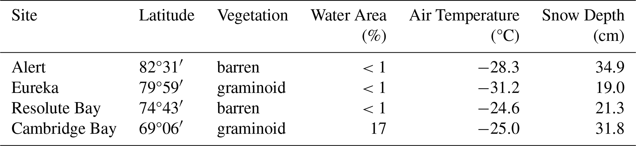
Four automatic weather stations (AWS) were identified across a latitudinal range in the Canadian high Arctic for this experiment (Fig. 1), selected because they are collocated with manual in situ SWE sampling sites. Basic site characteristics are provided in Table 1; including AWS climatology, predominant vegetation types from the Raster Circumpolar Arctic Vegetation Map (Raynolds et al., 2019), and area of nearby water bodies calculated with the HydroLAKES database (Messager et al., 2016). Following Royer et al. (2021)'s classification, three AWS sites – Alert, Eureka, and Qausuittuq (hereafter Resolute Bay) – are situated in the polar desert and Ikaluktutiak (hereafter Cambridge Bay) in the polar tundra. Sites in the polar desert are mostly barren and are exposed to harsh winter storms, but local topography around Eureka protects the area from storms creating a microclimate – described as a polar oasis, characterised by higher temperatures, lower precipitation, and more vegetation (Woo and Young, 1997). The Cambridge Bay site has more subarctic qualities featuring graminoid shrub vegetation and many small lakes nearby.

Table 1 Characteristics of study sites (average AWS air temperature and snow depth from 15 March to 15 April).

3 Data

3.1 Model Forcing Data

PM radiometry data were the main forcing for the proposed snow density retrieval algorithm. Radiometry data were acquired from the Advanced Microwave Scanning Radiometer Earth Observing System (AMSR-E) Calibrated Enhanced-Resolution Passive Microwave Daily Brightness Temperature Version 2 dataset (Brodzik et al., 2024), resampled to a 12.5 km EASE-Grid 2.0. PM observations spanned eight winter seasons (2003–2011) while the instrument was functional (reference snow density data were not available for the 2002–2003 season). AMSR-E observations for each station were extracted from an adjacent EASE grid cell to the AWS (highlighted in Fig. 1) to minimise water area in observation scene due to their proximity to the coast. Nighttime observations from the descending orbit track (∼01:30 a.m. local time at the equator) were used since snow conditions would be more likely to be cold and dry for optimal microwave retrievals (Derksen et al., 2005). Radiometry samples were smoothed with a 5 d Gaussian weighted mean filter as described by Holloway (1958). The 18.7 and 36.5 GHz vertically-polarised radiometer channels (hereafter 19 and 37 GHz, respectively) were used to estimate ΔT_b in the forward model.

Meteorological measurements, acquired from the Environment and Climate Change Canada (ECCC) AWS network were also used for model forcing. The electromagnetic snowpack model was parameterised with AWS data, which required daily measurements of snow depth and air temperature as prior snow conditions. AWS data were the limiting factor in this experiment because the network is sparsely distributed in northern Canada limiting potential sites.

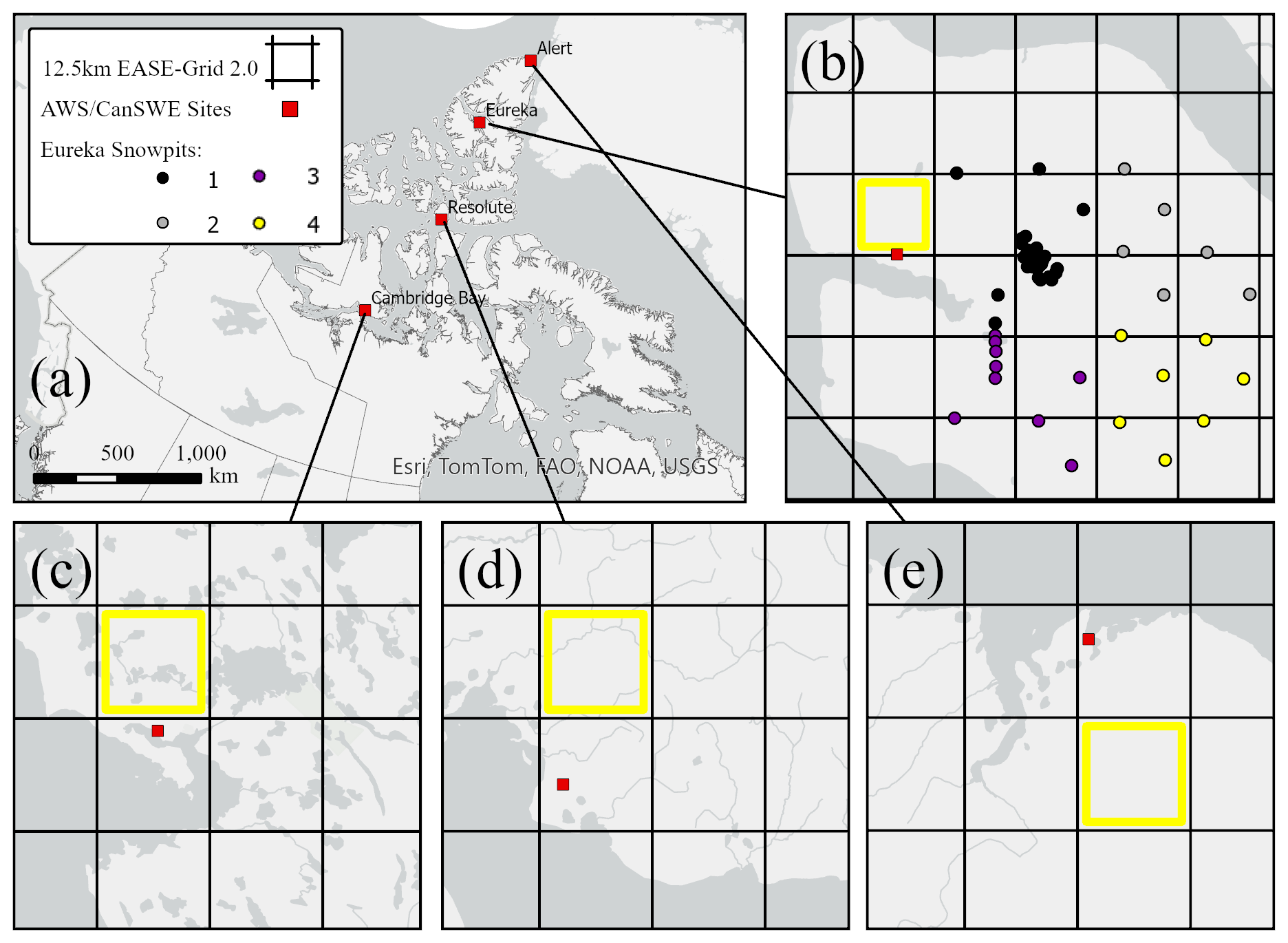
Figure 1 (a) AWS/CanSWE sites, distributed across the high Arctic in Nunavut, Canada, with insets showing 12.5 km EASE-Grid (highlighted cells used in analysis) for (b) Eureka (snowpit numbers correspond to Table 3), (c) Cambridge Bay, (d) Resolute Bay, and (e) Alert.

3.2 In situ Reference Data

3.2.1 Canadian Historical Snow Water Equivalent Dataset

The curated ECCC Canadian Historical Snow Water Equivalent dataset (CanSWE: Vionnet et al., 2021) provided in situ snow density data for algorithm calibration and evaluation. CanSWE was chosen because of its broad spatial coverage and relatively high temporal sampling frequency, although, it is recognised that snow density information from CanSWE is limited to bulk properties meaning they were unsuitable to evaluate algorithm estimates for individual snow layers. CanSWE included sampling locations collocated with AWS sites which allowed for direct comparisons of estimated and sampled snow density. Snow density data in CanSWE (considered in this study) were collected with ESC-30 SWE tubes along 5 to 10 point snow course transects spanning 150 to 300 m, aggregated into bulk estimates of snow density. A ten percent uncertainty range was applied to the snow density data in the reference dataset because of uncertainties inherent to manual snow density sampling (Conger and McClung, 2009; López-Moreno et al., 2020). Specific information about sampling procedures was not available for the individual sites in the CanSWE dataset (e.g. where the snow course is situated relative to the AWS was unknown).

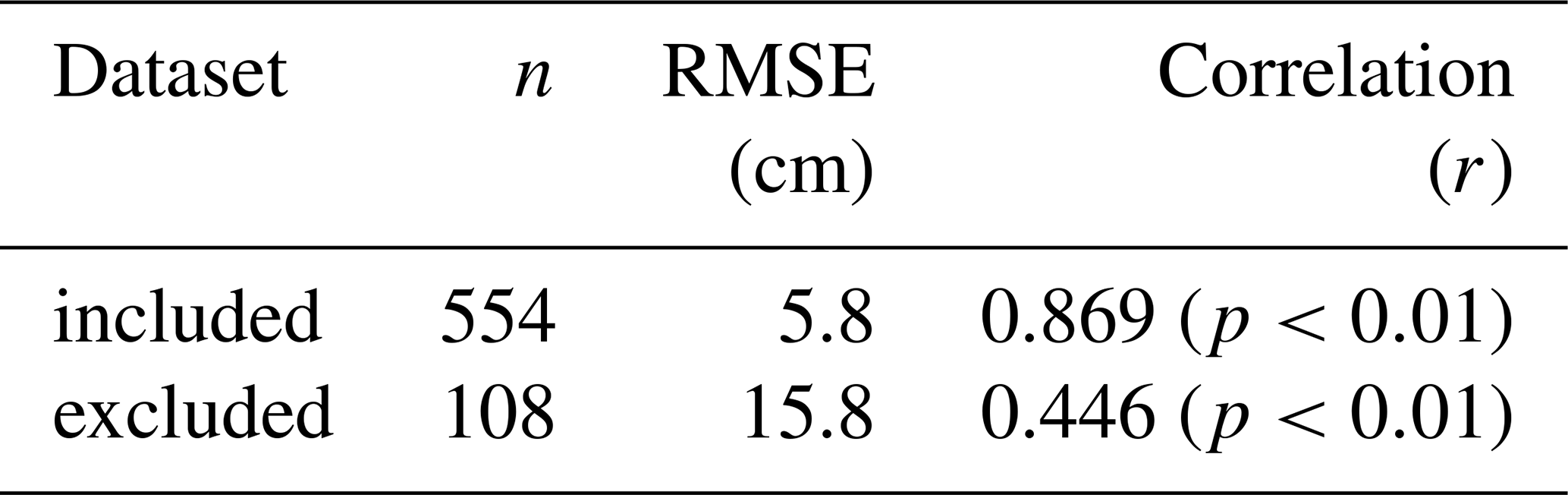
The reference dataset was limited with respect to the algorithm configuration (described in Sect. 4.4). Some yearly AWS forcing datasets were deemed unsuitable for algorithm forcing and were removed from the analysis. One winter season at the Eureka site (2008–2009) had insufficient snow accumulation to permit PM retrievals (i.e. <10 cm). Other datasets were excluded where snow accumulation trajectories reported by the AWS were substantially different from snow depth samples in CanSWE: three seasons for Alert (2007–2008, 2009–2010 and 2010–2011) and four for Resolute Bay (2003–2004, 2004–2005, 2005–2006, and 2006–2007) – otherwise, there was fairly good agreement AWS and CanSWE snow depths (Table 2). Individual CanSWE snow density samples were removed under three conditions: if they were out of the range of algorithm estimates (i.e. 150 to 450 kg m⁻³), if they were sporadic and did not fit temporally with the seasonal trajectory of the other samples, or if they were taken late in the season during the ablation period when the snowpack would likely be in a wet state inhibiting microwave retrievals.

Table 2 AWS and CanSWE snow depth comparison, which were included or excluded for model forcing.

3.2.2 Eureka Snow Survey Dataset

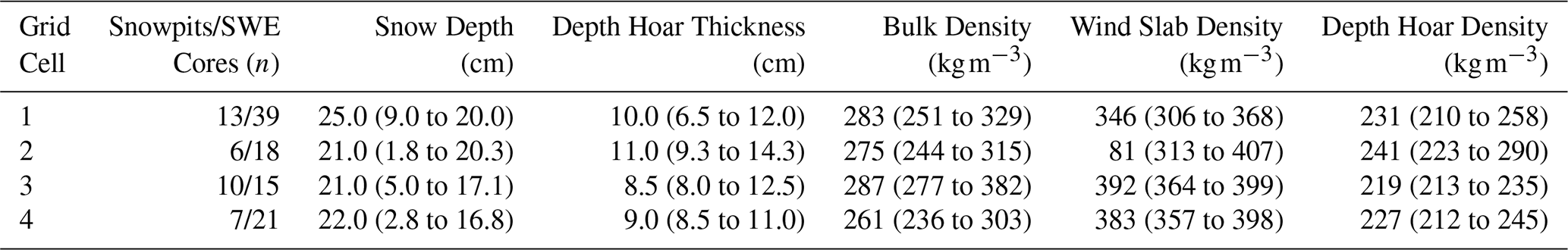
Due to the bulk nature of CanSWE density data, an additional dataset from Saberi et al. (2017) was used to evaluate algorithm estimates in greater detail. Extensive surveys of snow conditions were conducted near Eureka on the Fosheim Peninsula from 12–20 April 2011. The survey protocol was rather unique in terms of spatial extent covering four 25 km EASE-Grid cells, including stratigraphic data from snowpits and bulk snow properties from ESC-30 SWE tubes. Measured snow properties in each 25 km EASE-Grid cell were aggregated using median values (Table 3) to force algorithm retrievals and evaluate the algorithm configuration calibrated to bulk density measurements. Although limited to a single season, the Eureka snow survey dataset provided additional context to interpret algorithm outputs.

Table 3 Median (interquartile range) snowpack properties from Saberi et al. (2017) in each 25.0 km EASE Grid-cell – grid cell numbers correspond to points in Fig. 1b.

4 Methods

4.1 Electromagnetic Model

The Snow Microwave Radiative Transfer model (SMRT: Picard et al., 2018) was used as the forward model in the retrieval algorithm. SMRT was configured with the Improved Born Approximation (IBA) electromagnetic model (Mätzler, 1998) and microwave grain size microstructure model (Picard et al., 2022b), which have been demonstrated to be representative of high-Arctic snow conditions (Meloche et al., 2024). The substrate composition was parameterised to represent cryosolic soil following Meloche et al. (2021) and atmospheric contributions were estimated as described by Pulliainen et al. (1993).

The physically-based forward modelling approach required the snowpack to be parameterised, so the relevant characteristics needed to be quantified. A two-layer snowpack model was configured to account for the presence of depth hoar underneath a wind slab layer to best represent the microwave signature of tundra snow (Hall, 1987; Saberi et al., 2017). Upon initial deposition the snowpack would likely be in a homogenous state, with one layer, but that situation was not considered in this approach. The strong environmental controls present in the tundra contribute to the development of wind slab and depth hoar snow layers quickly after deposition (Benson and Sturm, 1993; Sturm and Holmgren, 1998), and algorithm retrievals were performed after 10 cm of snow had accumulated so the pack would be unlikely to be in the initial homogenous state.

4.2 Sensitivity Test

Microwave retrieval algorithms have traditionally estimated snow depth using a vertically polarised brightness temperature frequency difference (ΔT_b = 19–37 V), because of the sensitivity (insensitivity) of the 37 GHz (19 GHz) channel to snow accumulation, though we believe the same principle could be used to estimate snow density. Generally, ΔT_b is thought to increase with snow depth due to increasing volume scattering until a threshold after which the signal is saturated by thermal emission originating in the snowpack (Saberi et al., 2020). However, that is a simplified explanation of snow microwave interactions (i.e. only considering one layer) and can be complicated by stratification of natural snowpacks. For a tundra snowpack – with characteristic wind slab overlaying depth hoar – volume scattering is dominant for the depth hoar layer and non-scattering emission contributions originate from the wind slab (Sturm et al., 1993). Thus, it is important to understand how the properties of each snow layer would impact microwave emissions to design an effective snow density retrieval algorithm.

The electromagnetic model (described in Sect. 4.1) was used to simulate microwave emissions from tundra snowpacks to assess its sensitivity to various parameters. The electromagnetic model requires snowpack physical properties to be quantified, including thickness, density, specific surface area (SSA), polydispersity, and temperature of each layer. A series of experiments were designed to illustrate the effects of the various model parameters (representative of tundra snow, see Meloche et al., 2022; Picard et al., 2022b) and Arctic snow metamorphism; detailed descriptions of each experiment are provided in Table 4.

Table 4 Specific model parameters for wind slab (WS) and depth hoar (DH) layers in various sensitivity tests.

Snow density is our primary variable of interest, so it is important to understand how it effects microwave emissions. In the IBA model, scattering and absorption coefficients are in part related to snow density. The absorption coefficient increases linearly with snow density because of a greater proportion of ice-to-air in the microstructure representation altering the effective permittivity (Picard et al., 2018). On the other hand, the scattering coefficient has a non-linear relationship with snow density because of the interactions between individual scatterers in the snowpack. Volume scattering increases as more scatters are introduced (i.e. increasing density), until the scatterers are close enough in proximity to influence each other and the overall scattering efficiency decreases (Tsang and Kong, 2001). Thus, density of the wind slab and depth hoar layers can affect ΔT_b in different ways because of their properties that contribute to varying levels of volume scattering and thermal emission.

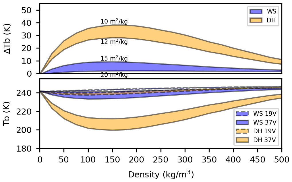
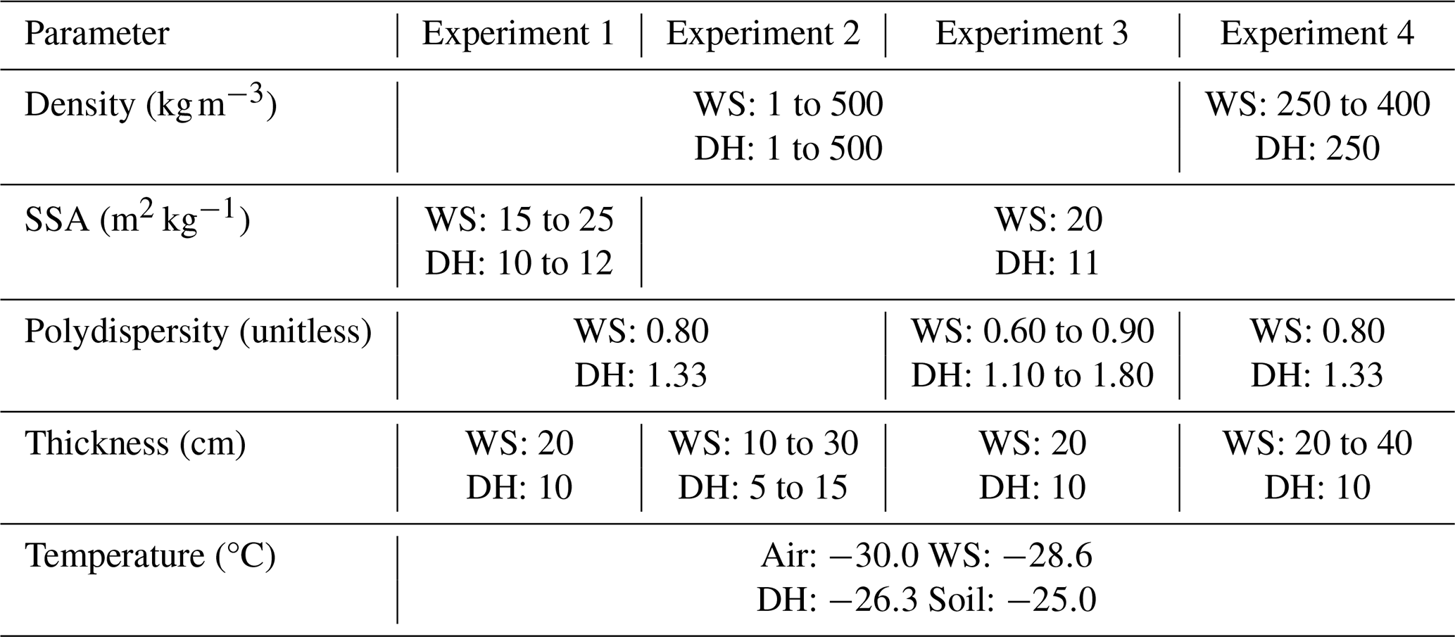
Figure 2 Experiment 1, simulated brightness temperatures of isolated WS and DH layers with variable density, shaded areas correspond to range of SSA values.

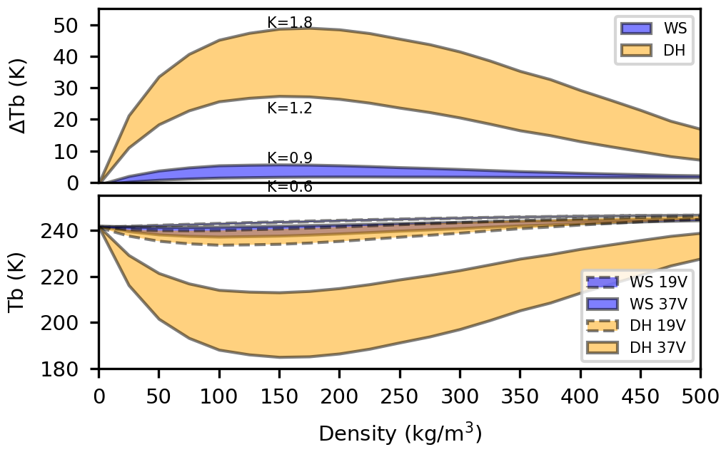
Figure 3 Experiment 2, same as Fig. 2 but shaded areas correspond to range of polydispersity rather than SSA.

Figure 4 Experiment 3, same as Fig. 2 but shaded areas correspond to range of thickness rather than SSA.

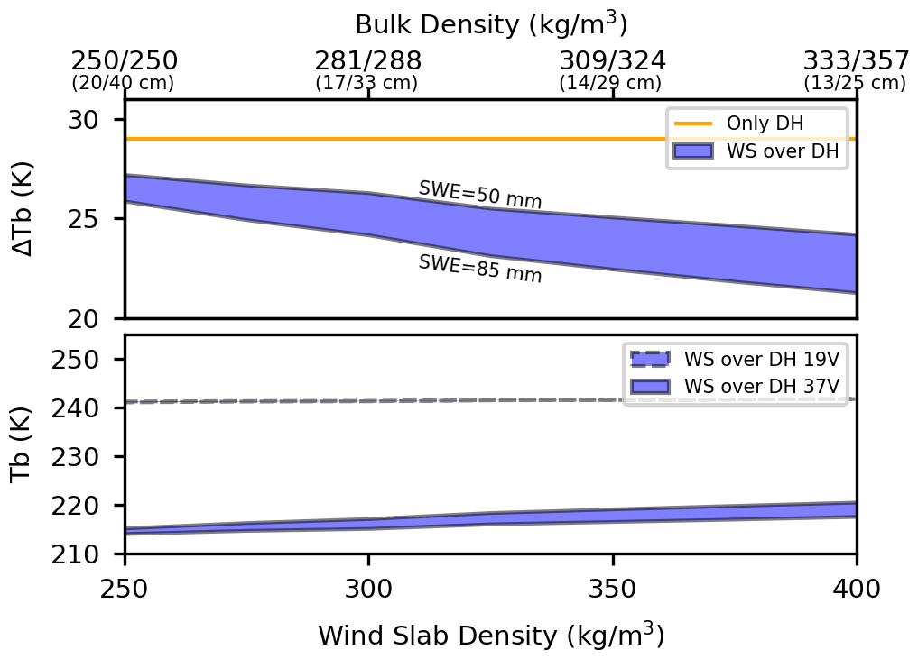
Figure 5 Experiment 4, simulated brightness temperatures of two-layer snowpack with variable wind slab density, mapped to bulk density (thin slab/thick slab), shaded areas correspond to range of wind slab SWE.

Experiments 1 to 3 were designed to simulate microwave emission from isolated wind slab and depth hoar layers, accounting for variations in SSA, polydispersity, and layer thickness, respectively (Figs. 2 to 4). The relationships between snow density and brightness temperatures follow skewed curves with minima at densities of 150 kg m⁻³ and frequency dependent amplitudes. Snow volume scattering is less sensitive to 19 than 37 GHz, so the frequency difference (ΔT_b) is approximately the reflected 37 GHz curve and its magnitude depends on different microstructure properties (Picard et al., 2022b). Lower (higher) SSA values produce greater (lesser) volume scattering, with minimal dependency on density, effectively translating the ΔT_b curves vertically (depth hoar ∼9 K between 10 to 12 m² kg⁻¹ and wind slab ∼3 K between 15 to 25 m² kg⁻¹). Similarly, polydispersity effectively scales SSA, also translating ΔT_b curves (depth hoar ∼19 K between 1.2 to 1.8 and wind slab ∼3 K between 0.6 to 0.9). Alternatively, layer thickness amplifies the relationship between snow density and simulated ΔT_b, increasing sensitivity to depth hoar density (∼10 K between 150 to 450 kg m⁻³ at 5 cm vs. ∼28 K at 15 cm) and the wind slab to a lesser extent (∼0.5 K between 150 to 450 kg m⁻³ at 10 cm vs. ∼3 K at 30 cm). Seasonal snow density is typical above the 150 kg m⁻³ inflection point (ignoring fresh snow), so we can assume snow density has a negative relationship with ΔT_b – with all other parameters equal, greater (lesser) ΔT_b would indicate lower (higher) snow density.

While there was minimal model sensitivity to the isolated wind slab in Experiments 1 to 3, the effect of the wind slab on brightness temperature should be more apparent when parameterised over depth hoar. Experiment 4 was designed to demonstrate brightness temperature sensitivity for the two-layer snowpack representation, configured to replicate mid-season wind slab compaction over an established depth hoar layer. Wind slab thickness was parameterised to decrease with compaction (i.e. densification) for SWE to remain constant, and a range of initial SWE values (i.e. thicknesses) were considered (shaded areas in Fig. 4). When introduced over the established depth hoar layer, absorption and thermal emission originating in the wind slab mask ΔT_b by several K depending on its SWE (∼2 K for 50 mm vs. ∼3 K for 85 mm). Then, absorption increased linearly with snow density and ΔT_b was accordingly masked by the wind slab as it compacted (∼5 K between 250 to 400 kg m⁻³ for 50 mm vs. ∼8 K for 85 mm). Thus, wind slab formation resulting from compaction or thickening should be apparent in AMSR-E radiometry (i.e. evident from decreasing ΔT_b), given its radiometric sensitivity of ±0.6 K. Furthermore, the magnitude of ΔT_b masking by the wind slab is enhanced by the snowpack thermal gradient and a relatively colder wind slab compared to the substrate will increase ΔT_b (∼2 K between 0 to −10 °C, not shown).

4.3 Snow Density Retrieval Algorithm

The results from the various experiments in the sensitivity test suggest there should be sufficient sensitivity to estimate snow density conditions from space-based PM radiometry. Further, PM radiometry was shown to be more sensitive to the thickness of depth hoar than the wind slab (and in turn overall snow depth) and, in terms of estimating Arctic snow mass, might be better suited to retrieving snow density rather than depth. PM retrievals of snow density were conducted at each AWS site, where meteorological conditions dictated when retrievals were performed. A minimum snow depth of 10 cm was imposed for algorithm retrievals because of the transparent nature of shallow snow to microwave emissions (Hall et al., 2002). Similarly, algorithm retrievals were not conducted when AWS air temperatures were above freezing because of the likelihood of liquid meltwater in the snowpack attenuating microwave emissions (Foster et al., 1984). With the AWS observations prescribed to the electromagnetic model an inverse modelling approach was applied to optimise the snow density parameters. The forward model was inverted by minimizing the cost function (J)

$$\begin{array}{}\text{(1)}& J({\mathit{\rho }}_{\mathrm{ws}},{\mathit{\rho }}_{\mathrm{dh}})=\left(\mathrm{\Delta }{T}_{\mathrm{b},\mathrm{sim}}\right({\mathit{\rho }}_{\mathrm{ws}},{\mathit{\rho }}_{\mathrm{dh}})-\mathrm{\Delta }{T}_{\mathrm{b},\mathrm{obs}}{)}^{\mathrm{2}}\end{array}$$

representing the vertically polarised 19 and 37 GHz spectral difference in the AMSR-E observation (ΔT_b,obs) and the simulated SMRT signature at the same channels (ΔT_b,sim), given the prescribed wind slab and depth hoar layer densities (ρ_ws and ρ_dh, respectively).

The solution to the two-layer snowpack model presented was imprecise because different layer density combinations could produce the same predicted ΔT_b in Eq. (1), resulting in a system with no global minima. The practical impact of this equifinality issue was that the algorithm may be confronted by seemingly equally valid but different layer density combinations, producing the same microwave signature. Without additional information there was no suitable way to identify the optimal layer density combination, so the retrieval algorithm was designed to solve for all microwave-plausible layer density combinations for a given observation scene to address equifinality in the inverse model.

To constrain the modelled layer density estimates to a plausible range, boundary conditions were established to limit the parameter space in which the algorithm could search for solutions to the inverse model. The first boundary condition was defined based on the strong environmental controls present in the tundra that result in a characteristic wind slab snow layer overlaying less dense depth hoar (Benson and Sturm, 1993). Logically, the wind slab layer should be denser than the depth hoar layer, so all parameter combinations where ρ_ws<ρ_dh were discarded, and the lower boundary situated where the densities of the two layers were equal. The second boundary for the model was defined based on the behaviour of microwave interactions in the electromagnetic model. Simulated ΔT_b peaks at a snow density of 150 kg m⁻³ (see Sect. 4.2), and the apparent permittivity in IBA is applicable up to a volume fraction of 50 %, or 458.5 kg m⁻³ (Picard et al., 2022a). Thus, the domain of each layer was limited to densities between 150 to 450 kg m⁻³ to ensure consistent behaviour in the electromagnetic snowpack model, and the upper boundary situated where either layer was at the edge of that domain.

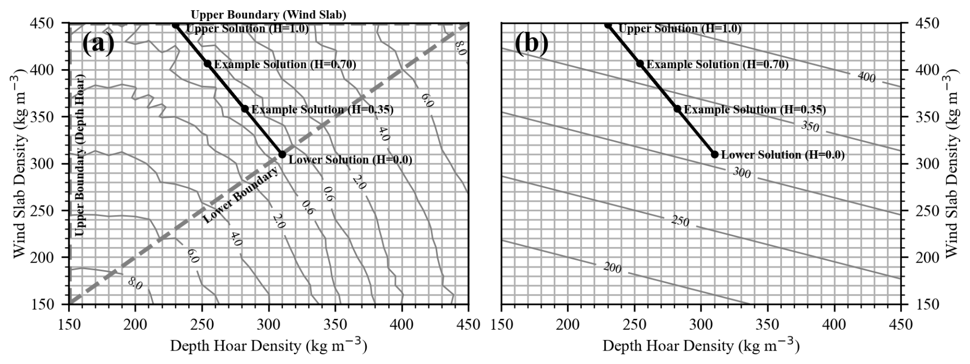
Figure 6 (a) Algorithm solutions for Eureka on 15 April 2011, with various H values, on surface defined by the square root of Eq. (1) in Kelvin, and (b) wind slab and depth hoar densities mapped to bulk values in kg m² with Eq. (4).

An important aspect of the retrieval algorithm was to exploit how the various minima on the cost surface, defined by Eq. (1), were positioned throughout the parameter space to reduce computational requirements. Figure 6 is an example of how the minima formed a valley transecting the parameter space. The microwave-plausible density range is shown in Fig. 6a as the set of layer density combinations situated along a straight line connecting the solutions at the two established boundary conditions for the inverse model. Wind slab and depth hoar density combinations were mapped to bulk values in Fig. 6b, where the contours of iso-density will pivot clockwise (counterclockwise) around the lower solution when the proportion of depth hoar thickness increases (decreases). It should be noted that under some instances, the valley could intersect the upper boundary related to the minimum depth hoar density (i.e. left axis in Fig. 6a), though the situation shown (intersecting the upper axis) was more common.

The lowest contour level (±0.6 K) in Fig. 6a represents the sensitivity of the AMSR-E radiometer at 19 and 37 GHz and the grid spacing corresponds to algorithm retrieval accuracy (10 kg m⁻³). In theory, the lower boundary can produce a solution with similar magnitudes of measurement uncertainty and retrieval accuracy (the upper solution is less precise being situated in a broader part of the valley). However, the stated radiometric sensitivity of the AMSR-E instrument is related to measurements of surface emission and additional uncertainty in the retrievals could be introduced because of atmospheric contributions. The atmosphere was configured to represent typical subarctic conditions (Pulliainen et al., 1993) but the frequency dependent relationship with water vapour content could change observed ΔT_b by ∼2 to 3 K from typical conditions. Thus, trends in snow density conditions should be apparent from spaceborne radiometry, with fluctuations from varying atmospheric water vapour content (partially mitigated with temporal filtering of PM radiometry); higher (lower) water vapour concentrations will cause the solution to shift towards the bottom-left (top-right) in Fig. 6a.

The range of microwave-plausible snow densities raised the question of how to evaluate the algorithm estimates against the reference data. A heterogeneity (H) parameter was introduced into the algorithm to estimate densities for the two snow layers and reduce the microwave-plausible snow densities to a single estimate of bulk snow density – ranging from 0 to 1 (i.e. the least and most heterogenous solutions, respectively). Wind slab (ρ_ws) and depth hoar (ρ_dh) densities were estimated related to H with

$$\begin{array}{}\text{(2)}& {\displaystyle }{\mathit{\rho }}_{\mathrm{ws}}={\mathit{\rho }}_{\mathrm{ws},\mathrm{lower}}+H\cdot ({\mathit{\rho }}_{\mathrm{ws},\mathrm{upper}}-{\mathit{\rho }}_{\mathrm{ws},\mathrm{lower}})\text{(3)}& {\displaystyle }{\mathit{\rho }}_{\mathrm{dh}}={\mathit{\rho }}_{\mathrm{dh},\mathrm{lower}}-H\cdot ({\mathit{\rho }}_{\mathrm{dh},\mathrm{lower}}-{\mathit{\rho }}_{\mathrm{dh},\mathrm{upper}})\end{array}$$

where (ρ_ws,lower, ρ_dh,lower) and (ρ_ws,upper, ρ_dh,upper) are the lower and upper solutions, respectively, and bulk density (ρ_bulk) estimated based on the depth hoar thickness divided by the total snow depth (depth hoar fraction, DHF)

$$\begin{array}{}\text{(4)}& {\mathit{\rho }}_{\mathrm{bulk}}={\mathit{\rho }}_{\mathrm{ws}}\cdot (\mathrm{1}-\text{DHF})+{\mathit{\rho }}_{\mathrm{dh}}\cdot \text{DHF}\end{array}$$

Ultimately, the bulk snow density estimated with H was treated as the final algorithm estimate with uncertainty defined by the microwave-plausible range.

4.4 Temporal Snowpack Parameterization

All existing retrieval algorithms have considered a single snow layer, so a new scheme was needed to parameterise the two layer snowpack model over the course of a season. Arctic snowpacks have been studied in detail during field campaigns (see Derksen et al., 2014; Meloche et al., 2022; Rutter et al., 2019), though they are mostly restricted to end-of-season conditions around March-to-April and much less is known about Arctic snowpack composition early in the season. There have been some studies that focused on early season conditions (Domine et al., 2016b, 2018), though they mainly provide qualitative descriptions of the temporal evolutions of Arctic snowpacks. Thus, our approach started with end-of-season conditions and worked backwards to parameterise the snowpack over the full season, with some parameters informed from available literature where possible and others calibrated.

Our temporal parameterization of snowpack properties was based on identifying trends in satellite PM and AWS observations, which we assumed to indicate different stages of snowpack evolution. Generally, two different behaviours were identified in the forcing datasets which we attributed to normal and restricted conditions for depth hoar development. In normal cases, ΔT_b increased rapidly over a short period in the fall immediately after the first snowfall, coinciding with an extended early season zero-curtain period producing extreme vertical temperature gradients for rapid depth hoar metamorphism (Domine et al., 2018). In restricted cases, ΔT_b increased gradually over longer periods of the season, consistent with high density layers slowly metamorphizing slowly into depth hoar (Derksen et al., 2009). Later in the season ΔT_b would plateau, attributed to a halt in depth hoar formation, before temperatures increase at end-of-season and ΔT_b drops rapidly.

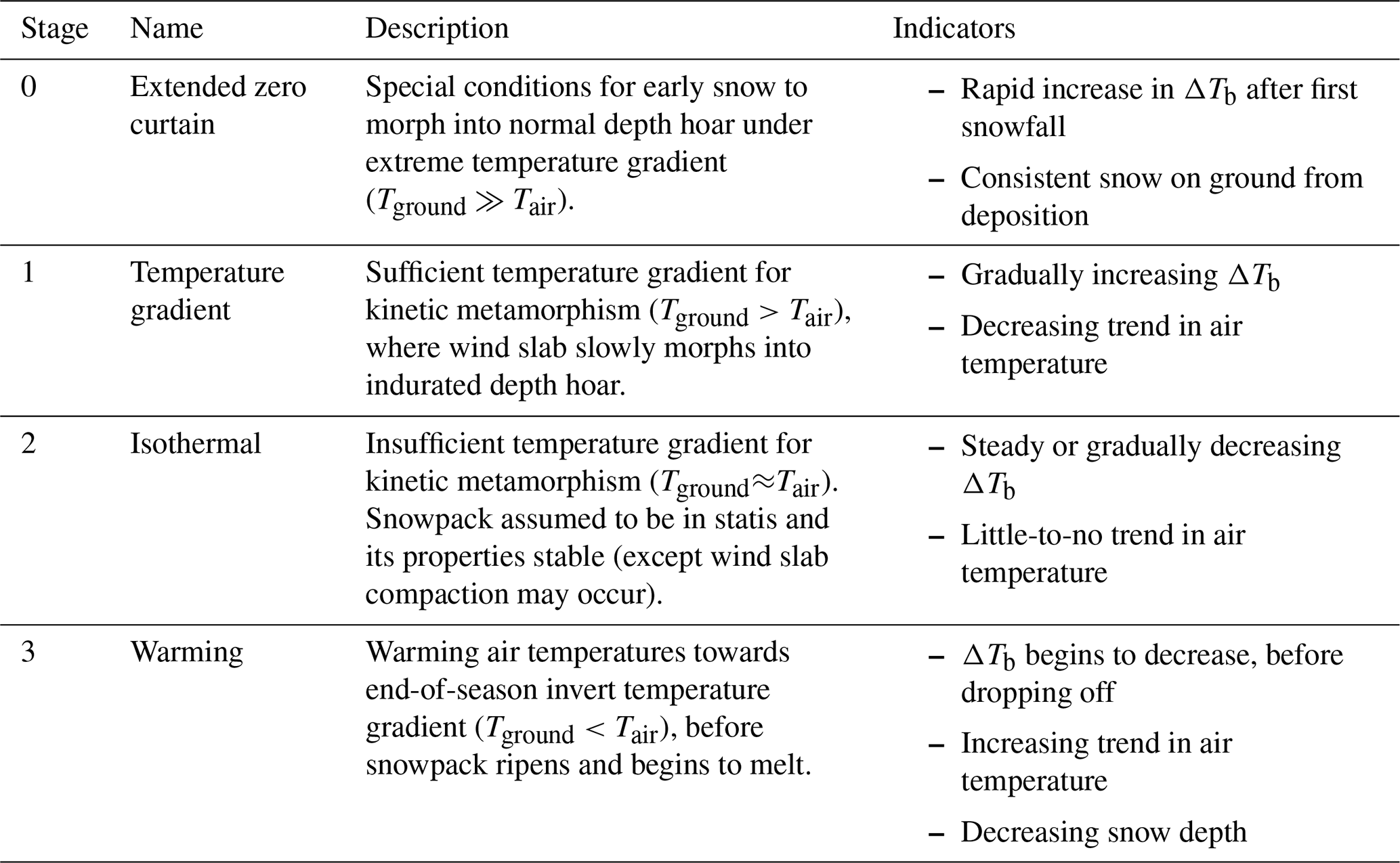
In total 4 different stages of snowpack evolution were identified, presented in Table 5. The proposed stages are numbered in the expected order of occurrence, but in practice their order can vary with some exceptions. Stage 0 is a special circumstance (i.e. does not happen every season) and must occur at the beginning of the season when temperatures are still around freezing. Then, the snowpack can alternate between Stages 1 and 2 throughout the season, owing to fluctuations in air temperature that change the thermal regime of the snowpack and snowfall events, prior to reaching equilibrium in State 2 towards end-of-season. Finally, the snowpack begins to warm in Stage 3 at the end-of-season with increasing air temperatures inverting the temperature gradient before ripening and final melt. The relevant state variables (i.e. layer thickness, thermal regime, and microstructure) were estimated dynamically considering the identified stage of snowpack evolution.

Table 5 Identified stages of snowpack evolution.

4.4.1 Depth Hoar Development

Basal depth hoar thickness is typically reported as a fraction of end-of-season snow depth (depth hoar fraction, DHF) and measurements during the early-mid season are limited in the Arctic. However, parameterizing the snowpack model accounting for DHF would cause issues. Forcing snow depth data should be representative of the observation scene (i.e. spatial resolution) and localised snow depth estimates (i.e. AWS) could lead to considerable differences in algorithm estimates given intrinsic variability in Arctic snow depth distributions (Liston, 2004). Additionally, depth hoar thickness parameterised with static DHF would likely be too thin during early-to-mid season, assuming the depth hoar layer should develop early on during shallower snow conditions relative to later in the season. Thus, we believe depth hoar should be parameterised with explicit thicknesses and a new approach was required for the prototype algorithm.

Our primary indicator of depth hoar development was based on seasonal trends in ΔT_b, with prolonged increases associated with depth hoar metamorphism (Derksen et al., 2010). Identifying periods of depth hoar development allowed rates of growth to be estimated. Rates were estimated with a change detection method that calculated cumulative increases in ΔT_b, similar to the Snow Index proposed by Lievens et al. (2019). The new index (depth hoar index, DHI) was predicated on the assumption any sustained increase (i.e. over multiple observations) in observed ΔT_b was proportional to depth hoar development. We believe depth hoar thickness should exhibit monotonic behaviour (i.e. increase, or remain constant, but not decrease), and temporary ΔT_b fluctuations would result from changes in the snowpack temperature gradient. The total contribution towards depth hoar development was estimated at each time step (t) with

$$\begin{array}{}\text{(5)}& {\displaystyle }\text{DHI}\left(t\right)=& {\displaystyle }\left\{\begin{array}{ll}\text{DHI}(t-\mathrm{1})+a\cdot \left[\mathrm{\Delta }{T}_{\mathrm{b}}\right(t)-\mathrm{\Delta }{T}_{\mathrm{b}}(t-\mathrm{1}\left)\right]& \text{if SD}>\mathrm{0},\\ \mathrm{0}& \text{otherwise}\end{array}\right.\text{(6)}& {\displaystyle }a=& {\displaystyle }\left\{\begin{array}{ll}\mathrm{1}& \text{if }\mathrm{\Delta }{T}_{\mathrm{b}}\left(t\right)\mathrm{\ge }\mathrm{\Delta }{T}_{\mathrm{b}}(t-\mathrm{1})\mathrm{\ge }\mathrm{\Delta }{T}_{\mathrm{b}}(t-\mathrm{2}),\\ \mathrm{0}& \text{otherwise}\end{array}\right.\end{array}$$

where AWS snow depth (SD) was used as an indicator of snow coverage and increases in ΔT_b must persist over multiple observations to mitigate effects from physical temperature fluctuations (handled with a from Eq. 6).

4.4.2 Layer Heterogeneity

The layer heterogeneity parameter (H) is abstract and was designed to represent the seasonal evolution of snowpack stratigraphy. Intuitively, values for H should begin near zero at initial deposition when the snowpack should be mostly homogenous and increase over time due to evolution of distinct layers. So, H was set to zero the first day snow on the ground was reported at the AWS and grew linearly to a maximum value calibrated for end-of-season conditions.

4.4.3 Snow and Substrate Temperatures

Operational SWE retrievals (e.g. Luojus et al., 2021) do not consider snow temperature gradient, though we believe it is important when thermal emission originating from the wind slab is considered. Thus, snow and substrate temperatures were required for the electromagnetic model but were not measured by AWS. Soil temperature from atmospheric reanalysis models were considered but their uncertainty is highest during cold seasons (Herrington et al., 2024). Instead, a model was designed to estimate soil temperature relative to measured air temperature and our identified stage of snowpack of evolution. In all stages, snow temperature was parameterised with a linear temperature gradient between air and soil temperature.

AWS daily mean air temperatures were used to replicate trends in substrate temperature at Arctic sites relative to air temperature measured by Domine et al. (2018). First, air temperatures were averaged over the previous 21 d to represent the gradual and lagged changes in soil temperature (general trend). Second, a 5 d Gaussian weighted mean filter was applied to air temperatures to represent the immediate effect of air temperature fluctuations (local trend). Then, the general and local trend estimates were assimilated with a 3:1 weighting scheme, respectively, together replicating how substrate temperatures should be partially decoupled from the atmosphere (insulated by snow cover) with small blips from large fluctuations in air temperature. Finally, the assimilated temperature trends were modified to account for the insulative properties of snow according to the identified phase of snowpack evolution: substrate temperatures were set to 0 °C during Stage 0, increased by 5 °C (2.5 °C) during normal (restricted) depth hoar development, and decreased by 5 °C (2.5 °C) during Stage 3, and the transitions between stages smoothed. The 5 °C value was chosen to represent the thermal insulation of normal depth hoar in line with mid-season tundra snowpack temperature gradients (Benson and Sturm, 1993), and an educated guess for the lower 2.5 °C value because of higher thermal conductivity for indurated depth hoar (Domine et al., 2016b). A comparison of estimates from this model to those from Domine et al. (2018) was provided in Appendix A.

4.4.4 SSA Decay

The microstructure model in SMRT (i.e. microwave grain size) required estimates of the SSA of ice grains in the snowpack which are not measured by operational AWS. Like depth hoar thickness, many more SSA measurements from Arctic snowpacks are available for end-of-season conditions, so empirical models were used to estimate SSA decay earlier in the season. New snow has relatively high SSA and decays logarithmically over time as it metamorphoses (Legagneux et al., 2003; Pinzer et al., 2012; Taillandier et al., 2007). Temporally varying SSA for depth hoar and wind slab were estimated using Eqs. (9) and (13) from Taillandier et al. (2007), respectively, with the general form

$$\begin{array}{}\text{(7)}& \text{SSA}\left(h\right)=B-A\cdot \ln \left(h+e^{\frac{B-{\text{SSA}}_{\mathrm{0}}}{A}}\right)\end{array}$$

where h is time since deposition in hours and coefficients A and B related to the mode of metamorphism, layer temperature, and initial SSA (SSA₀). Initial SSA was set as 50 m² kg⁻¹ and average layer temperatures calculated for the first 60 d after deposition as described in Sect. 4.4.3. Estimates of SSA from the empirical models were used until they reached predetermined values, representative of end-of-season conditions, to reflect the non-zero asymptotic trend in the evolution of depth hoar SSA (Taillandier et al., 2007) and very slow SSA decay in Arctic wind slabs observed later in the season (Domine et al., 2002).

4.5 Calibration and Evaluation Procedure

Some algorithm parameters could not be based on observations and instead needed to be determined through a calibration procedure. The calibration procedure consisted of two stages and ran each year from 15 March onwards, assuming snowpack properties would be mostly stable then. Calibrating for end-of-season conditions also allowed for parameters to be compared to those measured during field campaigns. First, wind slab SSA, depth hoar SSA, and depth hoar thickness were adjusted to produce the greatest overlap between the range of microwave-plausible snow density estimates and the in situ reference samples, with an overlap metric:

$$\begin{array}{}\text{(8)}& \text{overlap}={\displaystyle \frac{\mathrm{1}}{n}}\sum _{t=\mathrm{1}}^n{\displaystyle \frac{\left|\mathit{\right\{}{\mathit{\rho }}_{\mathrm{est}}\left(t\right)\mathit{\}}\cap \mathit{\{}{\mathit{\rho }}_{\mathrm{obs}}\left(t\right)\mathit{\left\}}\right|}{\left|\mathit{\right\{}{\mathit{\rho }}_{\mathrm{est}}\left(t\right)\mathit{\left\}}\right|}}\end{array}$$

where {ρ_est(t)} is the set of microwave-plausible estimated snow densities and {ρ_obs(t)} the corresponding CanSWE density sample with a ±10 % uncertainty range, at time t. Thus, the overlap metric described the proportion of the microwave-plausible snow density range that intersected the uncertainty range of the in situ samples, averaged over n time steps. Second, H was calibrated by converting the microwave-plausible algorithm estimates, from the first step, into discrete values to minimise mean absolute percentage error (MAPE). MAPE was chosen for this purpose, rather than absolute or squared error, because of the heteroscedastic nature of the uncertainty in the reference dataset.

At each site, algorithm snow density estimates were evaluated with CanSWE bulk density samples using the same metrics as in the calibration stage (i.e. overlap and MAPE); bias, root mean square error (RMSE), and correlation were also reported as indicators of algorithm performance. MAPE was treated as the primary measure of absolute accuracy of algorithm estimates – if MAPE was within the uncertainty range of the in situ samples (±10 %) then snow density estimates from the algorithm could be comparable to those collected with snow courses.

Calibrating the two layer snowpack model with bulk density measurements (i.e. CanSWE) introduced some uncertainty into the algorithm configuration parameters. As demonstrated by the sensitivity test, depth hoar SSA and thickness have complementary effects on simulated ΔT_b – i.e. lower (higher) SSA can compensate if the depth hoar is too thin (thick) – so various SSA and thickness combinations could produce similar microwave emissions. At each site, SSA parameters were kept constant over all seasons because inter-season variations in SSA should be relatively low (Meloche et al., 2022; Woolley et al., 2024), but DHF was free to account for varying environmental conditions. End-of-season H values were also kept constant for each site due to the lack of stratigraphic data to conduct a meaningful calibration and in an effort to reduce the number of free parameters in the calibration procedure. In the future, extensive stratigraphic data from multiple sites should be used for calibration to increase confidence in specific algorithm parameters.

5 Results

5.1 Calibrated End-of-Season Algorithm Configurations

Algorithm configurations were calibrated to represent end-of-season conditions, for each site some parameters were kept static over all seasons (Table 6) and depth hoar thicknesses varied each season (Table 7). The sensitivity test demonstrated the model was most sensitive to depth hoar parameters, so depth hoar SSA varied between 10.0 to 13.0 at increments of 0.2 m² kg⁻¹, and fewer options considered for the wind slab of 15.0, 17.5, or 20.0 m² kg⁻¹. For the polar desert sites (Alert, Eureka, and Resolute Bay) the calibration routine produced configurations that were fairly similar and in line with those expected in the polar desert, with depth hoar SSA around 10 to 11 m² kg⁻¹ and average DHF of approximately one third (Royer et al., 2021). On the other hand, the configuration for Cambridge Bay was different, with higher than expected depth hoar SSA and DHF for tundra type snow (Meloche et al., 2022).

Table 6 Model configuration parameters calibrated for end-of-season conditions.

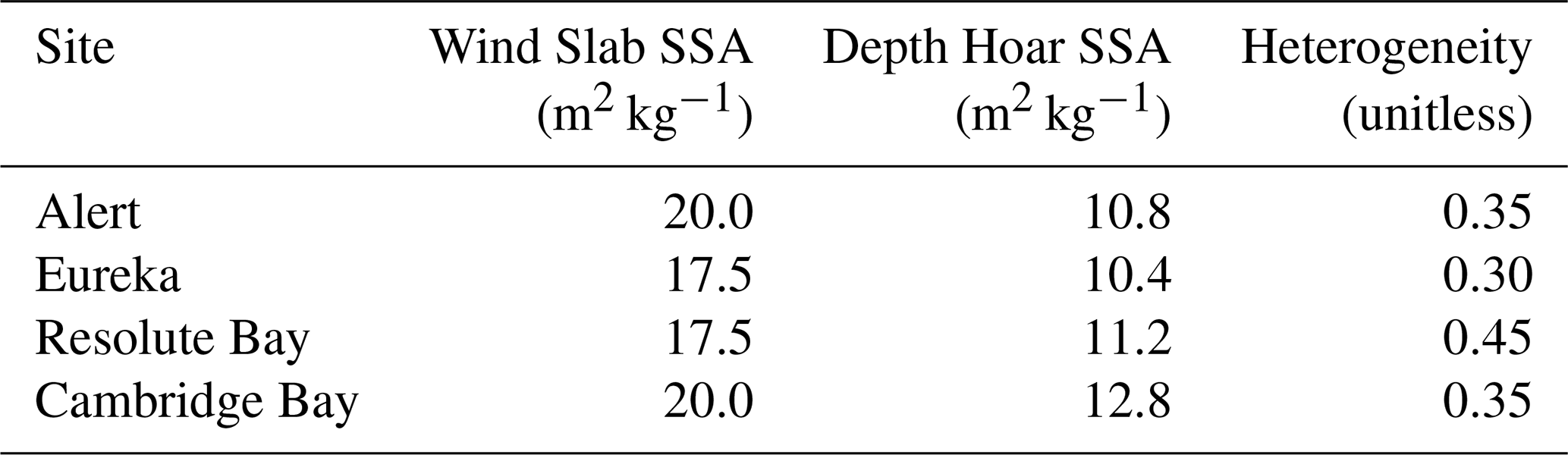
Table 7 Calibrated seasonal depth hoar thicknesses (cm) and percentage of end-of-season snow depth in parentheses.

5.2 Eureka Snow Survey Data

Snow survey data from Saberi et al. (2017) were used to evaluate the calibrated model configuration for the Eureka site in greater detail. The model was originally configured to replicate bulk density measurements (i.e. CanSWE) making it difficult to evaluate individual parameters without stratigraphic information. For example, simulated depth hoar thickness and SSA could compensate for one another without discernible differences in bulk density. Although SSA was not measured in the survey protocol, calibrated SSA values were evaluated by forcing the retrieval algorithm with measured layer thicknesses and AMSR-E L2A observations at 25 km (Ashcroft and Wentz, 2013), and the output compared to measured bulk, wind slab, and depth hoar densities (Fig. 7). Algorithm estimates showed good agreement with the measured values, though with slight overestimation for depth hoar and underestimation for wind slab densities. Interestingly, the valley of algorithm solutions for three gird-cells (1, 2, and 4) aligned with regions of iso-density in the parameter space (Fig. 6b) so H could increase slightly to reduce underestimation of wind slab density without affecting overall bulk density. While we cannot conclude from this limited sample size that the algorithm is perfect, the similarity of the algorithm estimates and layer densities to independent snow surveys suggest the parametrization of SSA was effective for Eureka.

Figure 7 Simulated and measured density for EASE-Grid cells near Eureka. Vertical error bars correspond to the microwave-plausible range of algorithm estimates and horizontal the interquartile range of measured values.

5.3 Dynamic Depth Hoar Parameterization

Snow depth and DHF can be variable in the tundra (Meloche et al., 2022), so parameterizing the snowpack model with static parameters could lead to uncertainty. Algorithm performance with calibrated depth hoar thicknesses were compared to those using generalised representations (i.e. seasonal thicknesses, average thickness, and average DHF from Table 6). Parameterizing the depth hoar layer with average thicknesses for each site improved algorithm estimates slightly compared to average DHF but the seasonal parameterization performed considerable better than either (Table 8). Further, seasonal depth hoar thicknesses were the only to bring algorithm estimates within the uncertainty range of the reference dataset at all sites (±10 %).

Calibrated seasonal depth hoar thicknesses were plotted against end-of-season DHI from Eq. (5). to identify a relationship to estimate dynamic depth hoar thicknesses (Fig. 8). Model configurations for each site should be equivalent (specifically depth hoar SSA) for a robust comparison of depth hoar thicknesses, so the configuration from Eureka was applied to the other sites since it seems representative of in situ conditions (see Sect. 5.2). Calibrated depth hoar thicknesses had a very strong relationship with DHI at Alert (R²=0.94, p<0.01), moderate relationships for Eureka (R²=0.68, p=0.023) and Resolute Bay (R²=0.64, p=0.20), and virtually no relationship for Cambridge Bay (R²=0.01, p=0.82). There was considerable spread in plotted values for Cambridge Bay and, when removed, the polar desert sites together have a very strong relationship (R²=0.93, p<0.01) fitted with a linear model

$$\begin{array}{}\text{(9)}& T_{\mathrm{EOS}}=\mathrm{0.349}\cdot {\mathrm{DHI}}_{\mathrm{15}\mathrm{Mar}}-\mathrm{3.75}\end{array}$$

allowing end-of-season depth hoar thickness (T_EOS) to be estimated in cm from DHI on 15 March (DHI_15 Mar).

Table 8 Algorithm performance metrics compared to CanSWE using calibrated configurations with depth hoar parameterised with seasonal thicknesses (seasonal), average thickness (avg. thickness), and average DHF (avg. DHF) from Table 6.

Figure 8 Depth Hoar Index from Eq. (5) plotted against calibrated depth hoar thicknesses and fitted linear models (lines).

5.4 Full Season Algorithm Runs

The temporal parameterization (described in Sect. 4.4) was used to force algorithm retrievals over full winter seasons. The calibrated configuration for Eureka was used for all sites and dynamic depth hoar thickness (DT) estimated in cm with

$$\begin{array}{}\text{(10)}& \text{DT}\left(t\right)=max\left(T_{\mathrm{EOS}}\cdot \left({\displaystyle \frac{\text{DHI}\left(t\right)}{{\mathrm{DHI}}_{\mathrm{15}\mathrm{Mar}}}}\right),T_{\mathrm{EOS}}\right)\end{array}$$

where DHI at time step t was from Eq. (5) and T_EOS from Eq. (9), and the maximum operator did not allow for growth after 15 March. Algorithm runs over all seasons at each site were aggregated to calculated performance metrics, presented in Table 9. Results for the three polar desert sites were similar with moderate MAPE (<20 %), weak-to-moderate positive correlations, and low magnitudes of bias, whereas, Cambridge Bay had higher MAPE, larger positive bias, and a weak negative correlation.

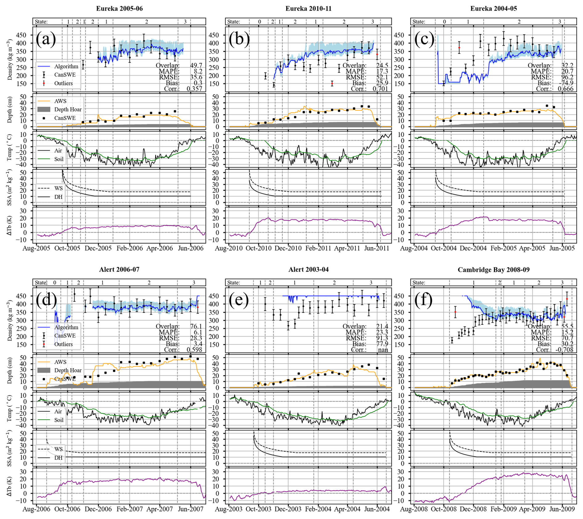
Figure 9 Example algorithm outputs (a–c) and forcing data (d–f), for (a) Eureka 2005–2006, (b) Eureka 2010–2011, (c) Eureka 2004–2005, (d) Alert 2006–2007, (e) Alert 2003–2004, and (f) Cambridge Bay 2008–2009.

A collection of notable algorithm simulations was included in Fig. 9 – some as examples of when the algorithm performed very well and others to demonstrate limitations – all simulations are included in Appendix B. Seasonal performance at Eureka was mixed, where three seasons had low MAPE (i.e. <10 %, e.g. Fig. 9a), 3 had moderate MAPE (i.e. <20 %, e.g. Fig. 9b), and one high MAPE (i.e. >20 %, Fig. 9c). The algorithm performed similarly at Alert, where three seasons had low MAPE (e.g. Fig. 9d), one moderate MAPE (not shown), and one high MAPE (Fig. 9e). Alternatively, algorithm performance at Resolute Bay was worse overall, where only one season had relatively low MAPE (not shown) and the other three had higher MAPE (not shown). Results for Cambridge Bay were more nuanced and the relatively high overall MAPE did not tell the whole story. In all but one algorithm run simulated density started considerably higher than reference samples in the early season but matched in situ samples very closely from February onwards (e.g. Fig. 9f).

Table 9 Algorithm performance metrics for full season runs relative to CanSWE samples (mean normalised percentage values in parentheses).

6 Discussion

6.1 Assessment of End-of-Season Configurations

In the following subsections, key parameters (i.e. SSA and depth hoar thickness) of the calibrated end-of-season configurations were compared against measured values from various field campaigns.

6.1.1 Eureka

Detail snow surveys from Saberi et al. (2017) were used to evaluate the algorithm configuration for Eureka. Calibrated depth hoar thicknesses for the Eureka site were fairly consistent ranging from 2.6 to 7.2 cm (σ=1.6 cm) and within the range of expected values for the polar desert (Royer et al., 2021). Simulated depth hoar thickness for the 2010–2011 season (6.7 cm) was comparable to measured values from the snow survey which had a median value of 9 cm (interquartile range of 6–12 cm). We expected thicker depth hoar from the snow survey dataset because it was focused around Hot Weather Creak, where conditions in the polar oasis should be more favourable for depth hoar formation. On the other hand, the manual snow survey course (i.e. CanSWE) was approximately 15 km west of Hot Weather Creak (Fig. 1b), so we believe conditions at the AWS should be somewhere between those found in the polar desert and polar oasis (i.e. relatively thinner depth hoar). Additionally, the calibrated SSA values produced representative estimates for individual layer densities measured during the snow survey (Fig. 7), increasing our confidence in the algorithm configuration for the Eureka site.

6.1.2 Alert

There were few snow survey data available for the Alert site (e.g. Domine et al., 2002), so those from relatively close Ward Hunt Island (∼170 km northwest) were also considered (Davesne et al., 2022). SSA values were similar to those measured by Davesne et al. (2022) but depth hoar was considerably thicker in some cases than the typical 5 to 10 cm expected in the polar desert (Royer et al., 2021). Further, there was considerable variability in simulated depth hoar thicknesses for Alert, with values ranging from 1.5 to 19.8 cm (σ=6.0 cm). Initially, we believed the large variability in depth hoar thickness to indicate an issue in the calibration routine (specifically higher values approaching 20 cm). However, variable depth hoar conditions have been recorded at Ward Hunt Island, which can be essentially devoid of depth hoar some years (Domine et al., 2018) or near 20 cm in other cases (Davesne et al., 2022). Thus, it appears the algorithm configuration for Alert was reasonable.

6.1.3 Resolute Bay

Snow survey data were available for Resolute Bay (Davesne et al., 2022; Royer et al., 2021), though the information was less specific than for other sites (i.e. no explicit depth hoar thickness). Simulated SSA values for the Resolute Bay site, like the others in the polar dessert, were with the range of expected values, but average DHF (17 %) was slightly lower than reported $\sim \mathrm{30}\pm \mathrm{20}$ % (Royer et al., 2021). Simulated depth hoar thickness was fairly consistent ranging from 0.9 to 5.4 cm (σ=1.6 cm) and DHF for all seasons (except 2010–2011) were within the range of measured values. Further, the area near Resolute Bay covered by the radiometer field-of-view was likely relatively dry, given its location inland with virtually no water bodies (Fig. 1d), and simulated DHF was comparable to values for dry areas surveyed by Davesne et al. (2022). Therefore, the algorithm configuration for Resolute Bay also appeared reasonable.

6.1.4 Cambridge Bay

Comprehensive reports of snowpack properties from Cambridge Bay (Meloche et al., 2022, 2024) allowed for detailed analysis of the calibrated algorithm configuration. Unlike the other sites, simulated depth hoar SSA and DHF were different for Cambridge Bay than field measurements (Meloche et al., 2022, 2024). The discrepancy between simulated and measured values could be related to water bodies around Cambridge Bay affecting radiometry (Derksen et al., 2010). However, we believe the issue to be mainly related to the complementary nature of depth hoar SSA and thickness towards volume scattering; with SSA values (wind slab: 20 m² kg⁻¹ and depth hoar: 11 m² kg⁻¹) from Meloche et al. (2022) calibrated average DHF (36 %) was very close to the reported value (38 %), and overall MAPE is only slightly higher (by 0.4 %). The possibility for large discrepancies between predicted and simulated parameters with little effect on simulated bulk density underscores the necessity for stratigraphic data during model calibration and evaluation.

6.2 Assessment of Temporal Parameterization

Estimation skill over the full season (Table 9) was lower than during the calibration stage (Table 8), though that was expected because the configuration for Eureka was used for all sites and depth hoar thickness was parameterised with Eq. (10) (rather than calibrated values for each site). In some cases the temporal parameterization produced excellent estimates of snow density over the whole season (e.g. Fig. 9a and d) but in other cases struggled to reproduce the observed densification trajectory (e.g. Fig. 9c and e). Yet, algorithm estimation skill at each site consistently improved over the course of a winter season and most algorithm estimates were close to the in situ references samples later on. To quantify this behaviour the reference dataset was partitioned into three temporal sets – October–November–December (OND), January–February–March (JFM), and April–May–June (AMJ) – and overlap, MAPE, and bias calculated for each in Table 10. There were substantial improvements in all metrics at all sites between OND to JFM and JFM to AMJ, and AMJ MAPE for the polar desert sites were within, or approaching, 10 % indicating the snow density estimation uncertainty was similar to the in situ samples. Temporal results for Cambridge Bay were slightly different than polar desert sites as there was a substantial improvement in all metrics from OND to JFM (most notably the reduction in bias) but MAPE increased in AMJ. Possible explanations for these temporal behaviours in algorithm estimates are discussed below.

Table 10 Seasonal performance metrics for algorithm snow density estimates relative to CanSWE, for October–November–December (OND), January–February–March (JFM), and April–May–June (AMJ).

The most likely reason for improved algorithm performance towards the end-of-season during most simulations is that the snow metamorphic state was captured effectively by model dynamics that align with our understanding of snowpack metamorphism. Prior knowledge from available literature increased confidence in end-of-season algorithm configuration, though much less was ready for the early-to-mid season introducing uncertainty into the temporal parameterization. Specifically, some properties were effectively quantified with physical models over time (e.g. SSA) while others were not because model representation is simply not developed (e.g. depth hoar thickness).

From the point of view of algorithm development, the most difficult element to parameterise over time was depth hoar thickness. The depth hoar model was generalised to not overfit to any specific forcing data, but edge cases were identified where there were issues. In some cases identified as standard development, and with thicker initial snow depth, Eq. (10) appeared to underestimate early-season depth hoar thickness causing simulated bulk density to pin at the bottom of the range to maximise volume scattering (e.g. Fig. 9c). That early-season underestimation could be related to how depth hoar was parameterised to grow vertically in thickness, which would be logical for indurated development (growing at the expense of wind slab thickness) but normal depth hoar should form from early layers morphing simultaneously. On the other hand, under the most restrictive conditions identified for depth hoar metamorphism Eq. (10) overestimated depth hoar thickness throughout the whole season casing algorithm estimates to pin at the upper limit of the density range to minimise volume scattering (e.g. Fig. 9e), despite very similar simulated (2.0 cm) and calibrated (0.8 cm) end-of-season thicknesses. Thus, our depth hoar model could be improved to consider specific situations – for example, initiating thickness with early-season snow depth measurements during Stage 0 (assuming the entire layer would shortly become depth hoar) and using a fixed thickness (∼1 cm) when very restrictive conditions are identified.

Even with the help of existing models there were challenges with the parameterization of SSA. Most notably, there is practically no distinction in the literature between standard and indurate depth hoar microstructure in terms of SSA and polydispersity, so we did not distinguish between their prescribed microstructure properties. While physical grain size of standard and indurated depth hoar are similar (Derksen et al., 2009), non-metamorphosed wind slab grains can be present in indurated depth hoar (Domine et al., 2016a); possibly leading to higher SSA or lower polydispersity compared to standard depth hoar, necessitating thicker simulated indurated layers. Further, our snowpack representation did not account for deposits of fresh snow, which have low density and high SSA, and, therefore, should be radiometrically negligible (Saberi et al., 2017). However, new snow was immediately incorporated into the simulated wind slab layer affecting simulated, but not observed, brightness temperatures – for example, mid-season snowfall events at Eureka in January 2011 (Fig. 9b) caused measured bulk density to decrease but simulated bulk density increased. Identifying depth hoar type with the proposed stages of snowpack evolution would not only aid in parameterizing algorithm retrievals (should their microstructure properties prove to be sufficiently different) but could also support applications where snow hardness and thermal conductivity are relevant – for example, permafrost thermal regimes and conditions for subnivean life (Domine et al., 2016a).

Algorithm estimates generally followed expected densification trajectories (i.e. increasing density over time) in the polar desert (e.g. Fig. 9b) but exhibited different behaviour at Cambridge Bay. Early season density estimates were too high in all, but one, simulations at Cambridge Bay and decreased over time to move closer to in situ measurements (e.g. Fig. 9f). Early season overestimation could be explained by penetration depth at 19 GHz exceeding lake ice thickness (Derksen et al., 2009), which reduced observed ΔT_b causing simulated density to pin at the upper limit to minimise volume scattering. Then, estimates improved over the mid-season when lake ice thickness should exceed the penetration depth at 19 GHz, before thinning ice thickness reintroduced uncertainty in observed brightness temperatures at the end-of-season (Derksen et al., 2009). Additionally, the radiometric influence of water bodies made it more difficult to interpret the stages of snowpack evolution at Cambridge Bay – Stage 0 was only identified during a couple seasons, despite tundra conditions being generally favourable for depth hoar development (Royer et al., 2021). Furthermore, unfrozen water bodies around Cambridge Bay caused pre-snow ΔT_b to be very low (i.e. negative ∼10 K) artificially modifying DHI values, likely contributing to the spread of points in Fig. 8. After February, when ice thickness should exceed penetration depth (Derksen et al., 2009), algorithm performance for Cambridge Bay was comparable to the polar dessert sites (MAPE = 13.2 % and overlap = 43.6 %).

6.3 Scalability Across the Pan-Arctic

The ultimate goal of this research is to develop a pan-Arctic snow density retrieval algorithm, though the algorithm would need to be modified for that purpose. The current retrieval design is predicated on a two-layer snowpack with distinct properties (i.e. found in the tundra/polar desert) and would need to be modified to consider other Arctic snow types (e.g. taiga). Traditional ecological knowledge of snow conditions (e.g. Riseth et al., 2011) could help to identify important snowpack parameters across various environments to be generalised for the electromagnetic model. Additionally, water bodies could impede retrievals using a ΔT_b approach (as described for Cambridge Bay) and a single channel retrieval using only 37 GHz might be more appropriate across the pan-Arctic (Derksen et al., 2010). Also, the dynamic depth hoar parameterization required PM observations from snow-on to 15 March limiting its use to retrospective analyses, though the relatively long PM observation record would allow for climatological analysis.

After necessary modifications, additional datasets would be required to expand the spatial extent of algorithm retrievals. Snow depth data are the most important to force the algorithm (after radiometry) and the sparse distribution of AWS across the pan-Arctic render them unsuitable for extensive model forcing. Spatially continuous snow depth estimates could be derived from reanalysis models, even as a first order effect, despite their uncertainty in high latitude areas where data are sparse (Cao et al., 2020). Assimilation of reanalysis snow depth estimates with AWS data for bias correction might be a promising way forward. Similarly, bias corrected ground temperature estimates from reanalysis products (Herrington et al., 2024) could replace our simple model based on AWS air temperature. Additionally, auxiliary wind speed and soil moisture data could aid with parameterizing the depth hoar layer (i.e. quantifying the potential for development) as they restrict and promote development, respectively (Davesne et al., 2022). Finally, a pan-Arctic snow density product would require extensive reference data to support algorithm calibration and evaluation which will need to be curated, specifically regarding extensive datasets of snow stratigraphy.

7 Conclusions and Future Work

A prototype algorithm was developed to estimate snow density in the tundra environment using PM remote sensing, given challenges in estimating spatiotemporally varying snow density in the Arctic environment. An experiment was conducted to assess the proposed algorithm's ability to estimate snow density at sites distributed in the Canadian high Arctic. Results from those sites demonstrate algorithm estimates have the potential to provided information on snow density comparable to those collected with in situ sampling. In its current configuration, the algorithm performed best at estimating snow density conditions later in the season, with end-of-season MAPE within (i.e. Alert and Eureka), or approaching (i.e. Resolute Bay and Cambridge Bay), the ±10 % uncertainty range of manual snow density sampling. With some modifications and more extensive forcing data the proposed algorithm could be applied across the pan-Arctic to provide snow density estimates at spatiotemporal scales that were not previously available.

The experimental design for this study was opportunistic due to the limited snow density data available for algorithm calibration and evaluation. CanSWE was the only readily available dataset which covered the required spatial and temporal domain for algorithm development but was limited to bulk estimates and, as result, estimates for the two distinct snow layers could not be sufficiently calibrated nor evaluated. Specifically, algorithm calibration with bulk density measurements introduced uncertainty in the parameterization of depth hoar thickness and SSA, because of their complementary effects on volume scattering. Future algorithm development will focus on datasets from sites with distributed stratigraphic measurements that will improve snow density parameterization at the PM scale. Further, Arctic snow conditions are known to be driven by terrain types (Rees et al., 2014; Woo, 1998) and we hypothesise the microwave-plausible snow density range for the PM scene could be disaggregated using high-resolution active microwave data to provide information on stratigraphic heterogeneity (replacing the abstract H parameter).

Appendix A: Comparison of measured and modelled substrate temperatures

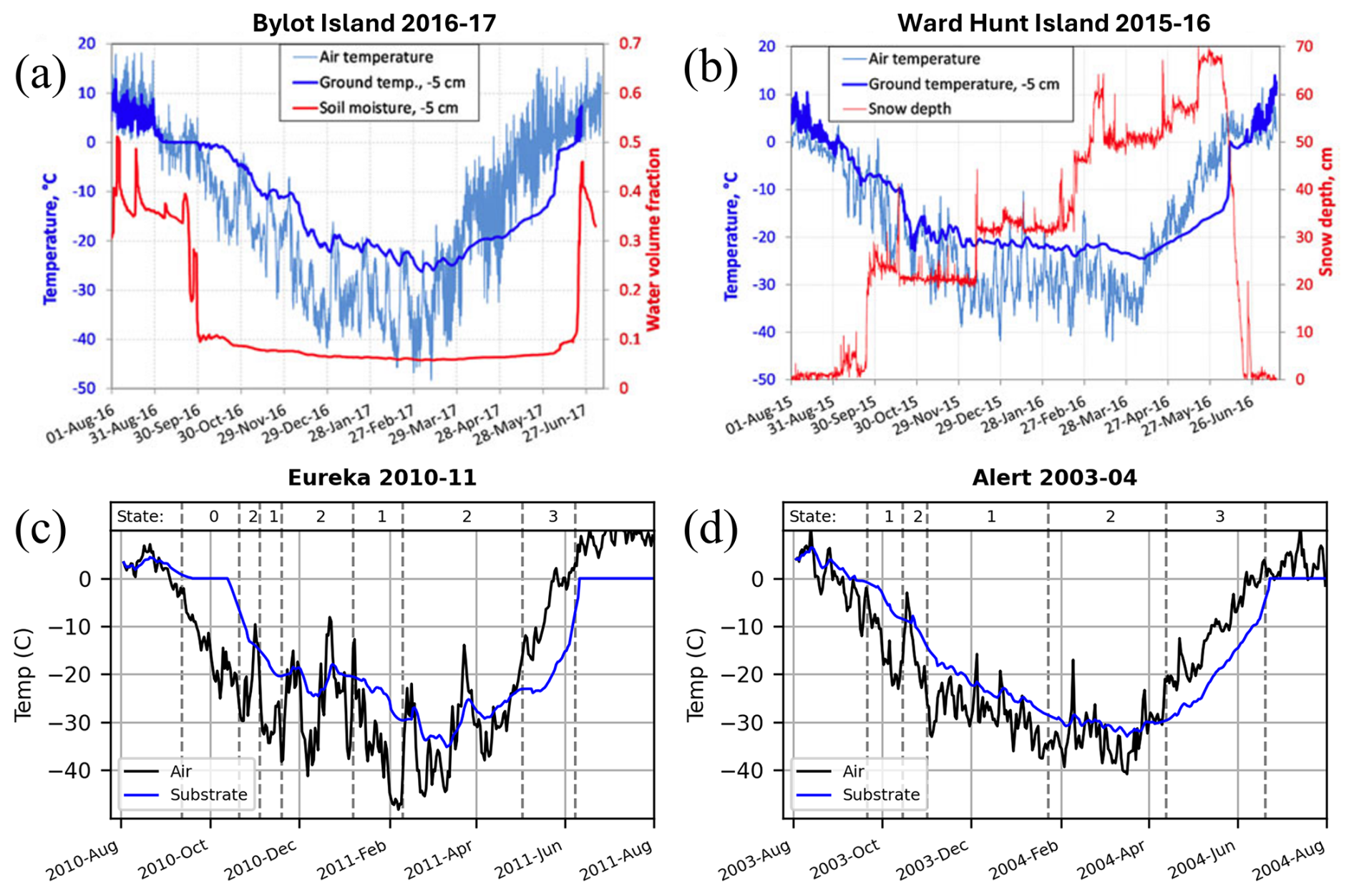
Figure A1 Air and substrate temperatures measured (adapted from Domine et al., 2018) at (a) Bylot Island 2016–2017 (normal depth hoar conditions) and (b) Ward Hunt Island 2015–2016 (restricted depth hoar conditions), and from our model (described in Sect. 4.4.3) under (c) normal depth hoar conditions at Eureka 2010–2011 and (d) restricted depth hoar conditions at Alert 2003–2004.

Appendix B: Algorithm Outputs

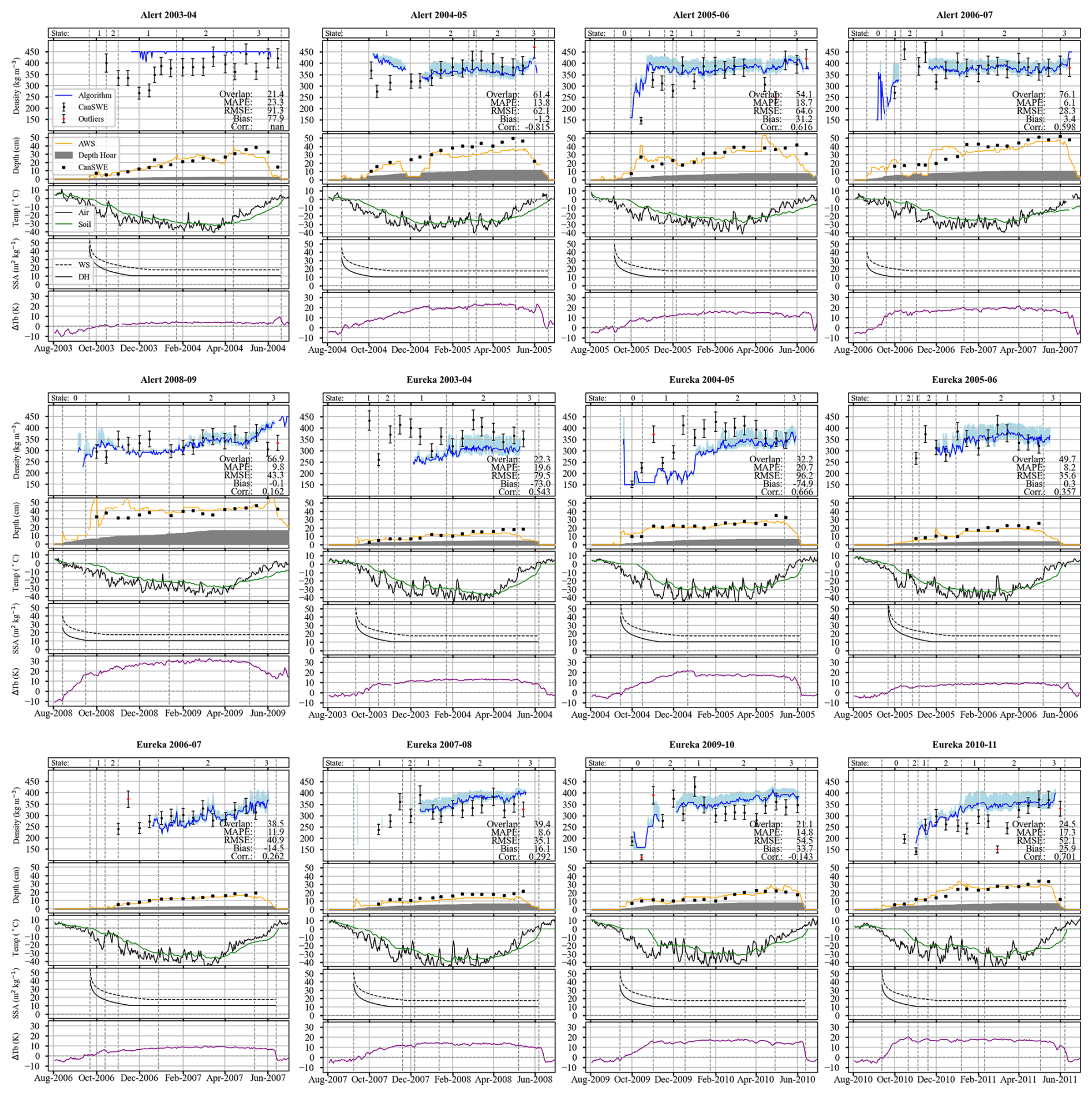
Figure B1 All algorithm simulations (top panel) and forcing data (lower panels) for Alert and Eureka sites (performance metrics same as those listed in Table 9).

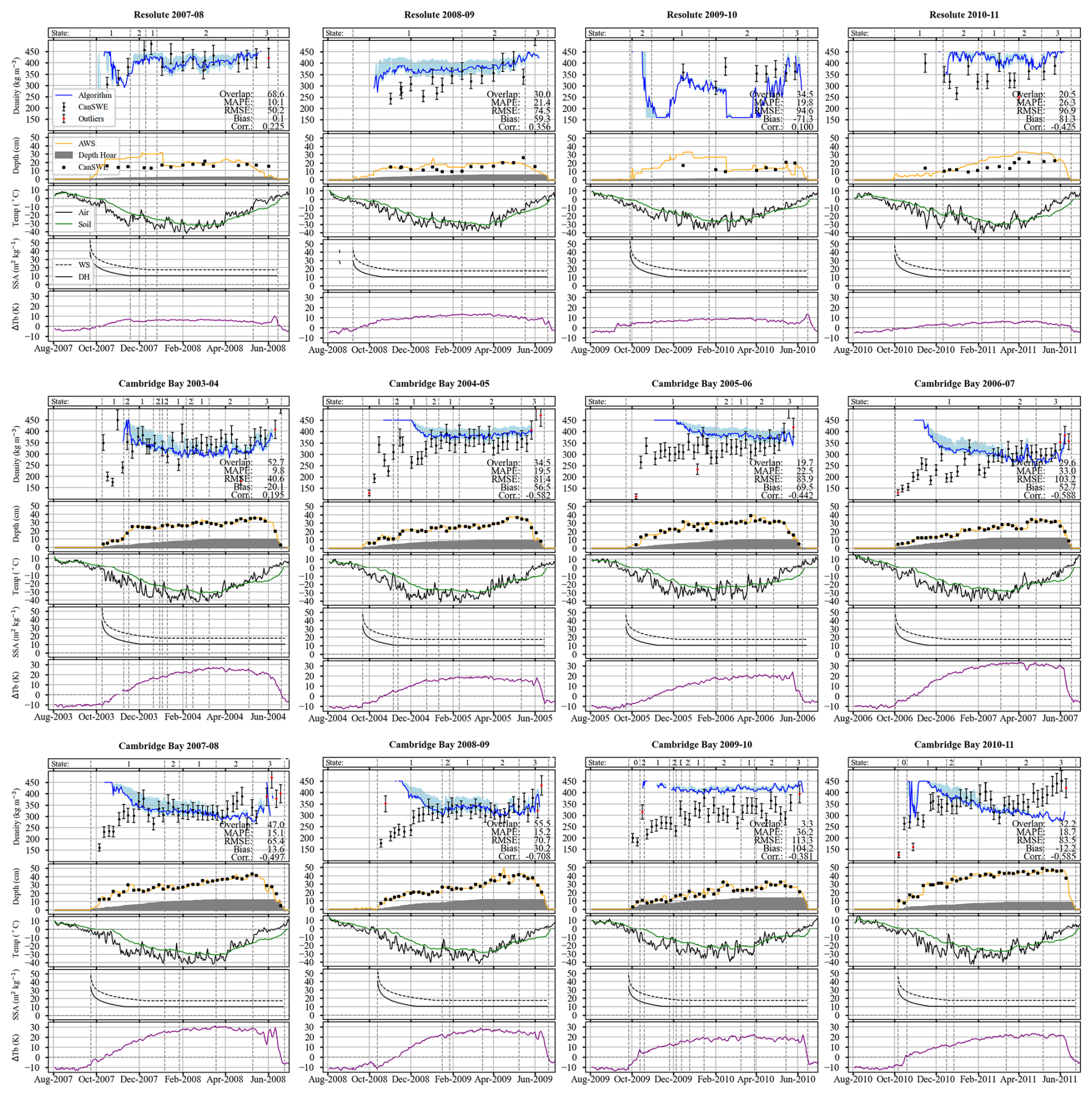
Figure B2 All algorithm simulations (top panel) and forcing data (lower panels) for Resolute Bay and Cambridge Bay sites (performance metrics same as those listed in Table 9).