On the statistical relationship between sea ice freeboard and C-band microwave backscatter – a case study with Sentinel-1 and Operation IceBridge

In this study, we evaluate the statistical relationship between sea ice freeboard and C-band microwave backscatter. By collocating observations between Sentinel-1 images and Operation IceBridge (OIB) measurements in April 2019, we evaluate their relationship under various sea ice types and thickness regimes. We show that, at various spatial scales relevant to synthetic aperture radar (SAR) observations, there exists an apparent significant correlation between C-band backscatter and sea ice freeboard. This relation depends on physical parameters of the sea ice, including the ice type, as well as sensor-specific parameters such as the observational incidence angle of the SAR satellite. As a result, there is considerable variability in this apparent relationship and its fitted parameters. Using the fitted relationship, two-dimensional freeboard maps can be predicted at the scale of SAR images' effective resolution (i.e., ∼ 200 m). More importantly, we demonstrate that although the resolution of SAR images are relatively lower than OIB freeboard maps, we can predict the high-resolution, meter-scale freeboard distribution where altimetry measurements are not available. Thus the representation of altimetric measurements can be improved with the upscaling based on the SAR image. The proposed method can be further utilized for the upscaling of satellite based sea ice topography measurements by the Ice, Cloud, and land Elevation Satellite-2 (ICESat-2). Related issues, including the limitation to spring data, scale dependency and the locality of the statistical relationship, as well as the upscaling of current and historical satellite campaigns, are further discussed.

1 Introduction

Polar sea ice has undergone drastic changes in response to global climate change (Kwok, 2018). As Arctic sea ice coverage diminishes at a substantial rate, there has also been a rapid decrease in ice thickness and volume (Sumata et al., 2023). In particular, sea ice topography, characterized by the small-scale sea ice height variability, has become smoother (Krumpen et al., 2025). Satellite altimetry serves as the backbone for observations of the circumpolar sea ice freeboard and thickness. For both laser and radar altimeters, the signals are sent from the satellites to Earth. By measuring the time difference between the emitted pulse from the satellite and the returned echo, the range between the satellite and the reflecting surface on Earth is estimated. The differentiation of the range of echoes returned from sea ice floes versus interstitial leads gives the radar or laser freeboard, and the sea ice thickness is then calculated from hydrostatic assumptions and the buoyancy relationship. In particular, NASA's ICESat-2 (IS2) satellite is a photon-counting laser altimeter that has carried out continuous observations in both polar regions since 2018 (Markus et al., 2017). Six laser beams of IS2 form into three strong-weak pairs, providing continuous ground coverage in the satellite's flight direction. Validation efforts with airborne campaigns that collocate with IS2 beam segments, including NASA's Operation IceBridge (MacGregor et al., 2021, OIB) and MOSAiC (Nicolaus et al., 2022), show that IS2 is able to achieve highly accurate measurements of the sea ice topography (Kwok et al., 2019; Ricker et al., 2023).

Despite their advantages, satellite altimeters have limited coverage over the sea ice cover. The spatial sampling is inherently confined within the nadir of the satellite's track. For example, the three IS2 beam pairs are within ∼ 3 km of its ground track. In order to attain basin-scale coverage, samples collected throughout the whole month are usually needed. However, within a month's time, the sea ice may have undergone significant changes due to both thermodynamic and dynamic processes. These changes cannot be represented by the aggregated monthly freeboard and thickness maps. Furthermore, the altimetric scans only cover limited area within typical passive microwave imagers' footprints, thus hindering the synergy with these observations (Xu et al., 2017).

In this paper we explore the potential of improving the laser altimeter's representation through a synergy with microwave backscatter measurements by synthetic aperture radars (SAR). In particular, the C-band SAR payloads onboard European Space Agency's (ESA's) Sentinel-1 (S1) satellites provide pan-Arctic coverage since 2014 through the Extra-Wide (EW) swath mode scans. In this study, we establish statistical relationships between OIB-based sea ice topographic and freeboard measurements and SAR backscatter normalized radar cross section (σ₀) from S1 scenes using collocated observations during April 2019. OIB flights during this month, in particular the Airborne Topographic Mapper (ATM) measurements, were intentionally collocated with IS2 tracks. The ATM measurements feature higher resolution and wider swaths than IS2 measurements, enabling the analysis of co-variability between freeboard and σ₀ at multiple scales. Therefore, they are used to study the upscaling of IS2 measurements. In Sect. 2 we introduce details of the data used and the processing protocols. Using these statistical relationships, we further design an algorithm prototype for SAR-based prediction and upscaling of laser altimetry, as comprehensively described in Sect. 3. And Sect. 4 covers the statistical analysis under various sea ice conditions. The locality and limitations of the prediction algorithm are also investigated, along with other related issues in Sect. 5.

2 Data and protocols

2.1 OIB campaigns in April 2019

During April 2019 four OIB campaigns were carried out in the Arctic (Fig.  1), which were collocated with IS2 and consequently provided validation data for the sea ice elevation (ATL07, see also: Kwok et al., 2019) and freeboard products (ATL10). In particular, the flights on 8 and 12 April were organized in a racetrack pattern and cover more than 200 km along the corresponding IS2 ground tracks, with outbound (i.e., northbound) and inbound (i.e., southbound) flight passes covering beam pair of #3–#4 and #1–#2, respectively. Two different types of conic scans of ATM onboard these OIB campaigns were carried out: the 15° wide swath scan that covers about 500 m across the flight pass, and the 2.5° narrow swath scan that covers about 60 m. The scan angle of the wide-swath scanners is 15°, resulting in a swath width of 500 m. The scan angle of the narrow-swath scanners is 2.5°, which enhances the shot density in the central part of the wide swath. In addition, there are three flight passes of the racetrack, and together they cover over 1 km in the cross-track/flight path direction. Furthermore, the campaign on 8 April dominantly covered areas with thick multi-year ice (MYI), while that on 12 April sampled more interstitial first-year ice (FYI) within the MYI. Two other flights on 19 and 22 April are longer tracks that traverse both MYI and FYI (Fig. 1). Based on ERA5 data for the study period, the large-scale atmospheric conditions were typical of the late-winter conditions in the respective regions. There were no sudden warming events or significant precipitation that potentially changes the SAR backscatter signature of the sea ice.

In order to fully utilize the ATM measurements on 8 and 12 April, we construct a merged sea ice freeboard map using all three OIB passes. The left and middle passes were about 1.25 h apart, while the right and middle passes were about 2.5 h apart. Full details of the processing are covered in Appendix A. Briefly, first, we retrieve the total freeboard (denoted F_s) within the entire ATM swath for each pass, using the raw elevation measurements by ATM. Second, we obtain the 1 m-scale F_s map for each pass through spatial linear interpolation. The scan pattern of the ATM results in a variable number of shot spacings within the scan swath, with relatively lower shot density in the middle (Petty et al., 2016). To mitigate uncertainty introduced by this spatial sampling non-uniformity, the irregularly spaced ATM elevation data are converted to a regularly spaced 1 m F_s map. Finally, the F_s maps of the three passes are stitched together after collocation, producing the F_s map that covers ∼ 1500 m in the cross-flight direction.

The standard OIB Level4 (L4) product includes F_s parameter derived from ATM measurements and geolocated aerial photography. It employs a lead discrimination algorithm, which utilizes geolocated aerial photography to identify local sea surface height, thereby enhancing the quality and number of sea surface height determinations. The final product is gridded to a 40 m along-track resolution and can serve as a validation reference for the newly constructed 1 m-scale F_s maps. Specifically, we coarsen the F_s map to match the 40 m resolution and the location (nadir to the flight) of the L4 product. Validations show strong agreement, with RMSE of 0.15 m on 8 April and 0.1 m on 12 April at 40 m scale. At 400 m scale, RMSE further decreased to 0.04 m on 8 April and 0.03 m on 12 April (Fig. S1 in the Supplement). Hence the 1 m-scale F_s maps are used further for the statistical analysis with SAR images.

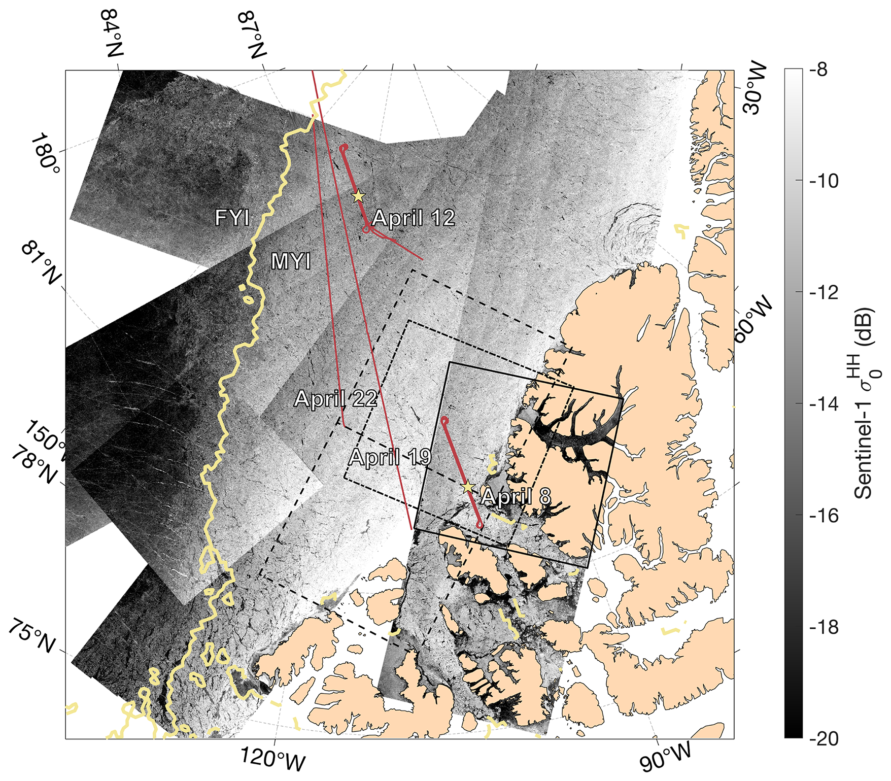
Figure 1 OIB campaigns during April 2019. S1 EW images collected around 8 April are shown in the background, with the black boxes outlining the images used for statistical analysis between C-band backscatter and sea ice freeboard. The solid box marks the boundary of the S1 image on 8 April, while the dashed (dot-dashed) ones mark those on 7 April (9 April). The OIB ground tracks of the 4 d are marked by red lines, and the location of the 9 km sample segments are shown by the asterisks. The thick yellow line delineates the boundary between the MYI and the FYI regions according to the sea ice type product provided by the Ocean and Sea Ice Satellite Application Facility (OSI-SAF).

2.2 S1 EW images and sea ice type maps

Both S1A and S1B data are available during the study period of April 2019. EW mode images with dual polarization channels (HH and HV) are accessed and collocated with the aforementioned OIB observations. The SAR incidence angles (IA) across the swath range from 20 to 46° for S1's EW mode. EW mode images use TOPSAR techniques to achieve a very large swath coverage (∼400 km), but TOPSAR acquisitions are affected by the “scalloping effect” (De Zan and Guarnieri, 2006). Additionally, the noise floor varies with range position, creating discontinuous sharp intensity changes known as the “banding effect” (Lohse et al., 2021; Sun and Li, 2021). These issues are particularly prominent in the HV-channel due to its low signal-to-noise ratio (SNR) (Segal et al., 2020). Details of the SAR images, including the image identifiers and the acquisition times, are provided in Table B1. Each image is preprocessed using ESA's Sentinel Application Platform (SNAP, version 11.0.0). Processing steps include the application of precise orbit files, thermal noise correction, radiometric calibration, and terrain correction. Finally, we convert the backscatter intensities into σ₀. It is important to note that in this study we did not apply IA corrections to the SAR images. There are several reasons: First, the IA dependency is type-dependent, with deformed ice showing lower sensitivity to IA than level ice (Makynen et al., 2003). Given the variant ridge density within the SAR's footprint (∼ 100 m), a simple correction for IA is insufficient in our study. Second, for the SAR image on 8 April, the IA change was within 10° along the whole OIB track, and on 12 April, IA values were within 5°. Since the range of IA is small, the correction has potentially limited effect on our study. Third, the best angle for the IA correction should be chosen to maximize the differentiation among different ice types. What is the best angle remains an open question and requires more systematic study.

Sea ice type information is derived from S1 images and the sea ice classification algorithm used in this study is based on: Lohse et al. (2020) and Guo et al. (2025). Lohse et al. (2020) developed a supervised algorithm that accounts for the class-dependent IA effects, known as the GIA classifier. While this classifier performs well in addressing IA sensitivity, some misclassifications and ambiguities remain. To address these issues, Guo et al. (2025) enhanced the algorithm by incorporating GLCM texture features, resulting in improved class separation. This study uses this classification approach to produce sea ice type maps on the selected S1 scenes.

In the classification process, seven GLCM textures are derived from the HH-channel of each SAR image, with a texture window size of 11 pixels. Then, SAR intensities (HH and HV) and GLCM textures (HH) are used as input to the GIA classifier, which incorporates their IA dependencies. Sea ice is classified into three types: level first-year ice (LFYI), deformed first-year ice (DFYI), and multiyear ice (MYI). To further refine the results, a Markov Random Field based contextual smoothing process is applied with a window size of 3 pixels (Doulgeris, 2015). The final sea ice type maps have a pixel size of 40  m, but their effective spatial resolution is significantly coarser due to SAR speckle filtering and textural processing. Sea ice classification is carried out for all the S1 images and the results are used for further analysis.

By default, the S1 images are projected to 40 m spatial resolution, which is the nominal pixel spacing of the S1 EW medium GRDM mode data, though the effective resolution is approximately 90 m. In addition, the processing steps in SNAP may further degrade the resolution of the σ₀ map. This is because a Single Product Speckle Filter with a sliding window of 7×7 pixels wash applied during the speckle filtering process (Mansourpour et al., 2006). We use the following notations for the coarsened values: ${\stackrel{\mathrm{‾}}{F_{\mathrm{s}}}}^{\left(s\right)}$ and ${\stackrel{\mathrm{‾}}{{\mathit{\sigma }}_{\mathrm{0}}}}^{\left(s\right)}$, where s denotes the coarsening scale.

2.3 ICESat2 products

The official IS2 products (version 6) are accessed for the collocating tracks with OIB campaigns on 8 and 12 April (see Data Availability for details). Each of the beam segments are of about 150 aggregated photons, and the mean sea ice elevation of each segment is provided in ATL07. Due to the variable photon rates over the sea ice, the along-track length of the beam segment is not constant, around 10–16 m. It is also different between strong and weak beams, with the beam segment length of the weak beams at about 50 m. In this study, we use the footprints of both the strong and weak beam segments to study practical issues limiting the upscaling of IS2 measurements, extending our analysis from OIB to lower freeboard resolution.

2.4 Ancillary datasets

The climate data record of global sea ice drift from the Ocean and Sea Ice Satellite Application Facility (OSI-SAF, version OSI-455) is used as the reference to the collocation of the different datasets. The OSI-455 product is available for the period of 1991–2020, and is derived from various passive microwave sensors (SSM/I, SSMIS, AMSR-E, and AMSR2) and wind field data from an atmospheric reanalysis. The sea ice drift vectors are provided on the Equal-Area Scalable Earth (EASE) grid with the spatial resolution of 75 km. However, they are not available near the shoreline (i.e., part of the campaign on 8 April near the Canadian Arctic Archipelago). The temporal scale of the drift vectors is 24 h, starting/ending at 12:00 UTC (Lavergne and Down, 2023).

2.5 Collocation between OIB and S1 images

The collocation between the F_s maps and σ₀ in the HH-polarization channel is carried out to correct for potential sea ice drift and geocoding uncertainties between the two measurements. The OIB flight on 8 April was approximately 40 min apart from its corresponding S1 image acquisition, whereas the OIB flight on 12 April was about 4 h apart from its respective S1 image acquisition. For the OIB flight on 8 April, the ice surveyed was relatively immobile, while that covered by the campaign on 12 April experienced a drift of approximately 0.02 m s⁻¹ according to the OSI-455 product. We coarsen the 1 m-scale F_s maps to the nominal pixel size of S1 EW images (i.e., 40 m), and maximize the correlation (Pearson's r) between the two fields by locally adjusting the relative location between the two. The increments of the local adjustments is 20 m (i.e., half of S1 EW pixel spacing). When collocating OIB tracks with S1 images, we divided the OIB tracks into 9 km segments. Collocation is performed independently for each 9 km outbound and inbound segment, in both the along-track and cross-track directions. In order to compare to the drift corrections during the correlation maximization (see Figs. 4a and 5a), the daily OSI-SAF drift vectors are scaled to the time interval between the acquisition time of the SAR image and that of the OIB. Afterwards, bilinear interpolation is carried out in the spatial domain to attain the drift vector at each location along the OIB flight path.

3 Methods

3.1 The statistical fitting between the F_s and σ₀

To analyze the statistical relationship between F_s and C-band backscatter, we employed a linear regression model for each 9 km segment (both outbound and inbound), defined as: $\stackrel{\mathrm{‾}}{F_{\mathrm{s}}}=a\cdot {\mathit{\sigma }}_{\mathrm{0}}+b$. Sea ice type maps, which classify the sea ice into LFYI, DFYI, and MYI, were used. During the classification, a sliding window of 11 pixels was applied in the classification process; if all pixels within an 11×11 window were of the same type, the central pixel was classified as a pure pixel (indicated by solid circles in Figs. 2d–i and 3d–i); otherwise, it was labeled as a mixture(indicated by square symbols in Figs. 2d–i and 3d–i). We specifically examined the relationship between F_s and backscatter for pure MYI pixels. Due to the limited number of pure FYI and DFYI pixels, these were not included in further analysis.

Backscatter values were binned into 1 dB intervals. For each bin, the mean F_s value within the interquartile range (IQR) was calculated. The representative backscatter value for each bin was determined as the mean of the bin boundaries. The statistical relationship between these mean F_s values and representative backscatter values was then analyzed.

Since the effective resolution of the backscatter used in this study is larger than 40 m, coarser spatial scales adopted for the computation of $\stackrel{\mathrm{‾}}{F_{\mathrm{s}}}$, including 100 m (Fig. 2e and h) and 200 m (Fig. 2f and i).

3.2 F_s distribution prediction

The prediction of F_s distribution is based on 1 m-scale samples for OIB and beam-segment scale for IS2. The training of the prediction algorithm is carried out as follows:

1. Bin backscatter values into 1 dB intervals.

2. For each bin, calculate the mean F_s value within the IQR.

3. Use the three-component Log-Logistic mixture distribution to fit the F_s sample probability density function (PDF) within each σ₀ bin. The probability density function of the three-component Log-Logistic mixture distribution is given by:

   $$p\left(x\right)=\sum _{i=\mathrm{1}}^{\mathrm{3}}{\mathit{\omega }}_i\cdot {\displaystyle \frac{({\mathit{\beta }}_i/{\mathit{\alpha }}_i)(x/{\mathit{\alpha }}_i{)}^{{\mathit{\beta }}_i-\mathrm{1}}}{(\mathrm{1}+(x/{\mathit{\alpha }}_i{)}^{{\mathit{\beta }}_i}{)}^{\mathrm{2}}}}$$

   where ω_i is the weight, β_i is the shape parameter, and α_i is the scale parameter for the ith Log-Logistic component.

4. Apply the maximum likelihood estimation (MLE) method to fit the Log-Logistic mixture model. Identify the optimal parameter estimates by maximizing the likelihood function of the sample data under the hypothesized Log-Logistic mixture distribution. Transform the problem of maximizing the likelihood function into minimizing the negative of the likelihood function. Then, solve this optimization problem using the sequential quadratic programming (SQP) algorithm.

To evaluate the goodness-of-fit between the sample distribution p(x) and the fitted three-component log-logistic mixture distribution $\stackrel{\mathrm{̃}}{p}\left(x\right)$, we employed the Kolmogorov-Smirnov (K-S) distance, defined as:

$$\underset{x}{sup}\left|P\right(x)-\stackrel{\mathrm{̃}}{P}(x\left)\right|$$

Here, P(x) and $\stackrel{\mathrm{̃}}{P}\left(x\right)$ denote the cumulative density function of the sample and the fitted distributions, respectively, and sup_x the supremum of the difference between the two. The K-S distance ranges between 0 and 1, with higher value indicating larger discrepancy between the distributions. We further used the k-means algorithm for the clustering analysis of these components in all σ₀ bins, and related them to different sea ice types.

For the test of the prediction algorithm, we train the prediction model with the inbound segment, and carry out the prediction and validation on the corresponding outbound segment. For OIB tracks, the 9 km segment length is adopted, while for IS2, due to limited beam segment samples, the longer segment length of 27 km is adopted. For each σ₀ on the outbound segment, we use the fitted F_s distribution on the corresponding σ₀ bin on the inbound segment for the prediction. The predicted F_s distribution for each σ₀ sample is combined for all SAR pixels on the outbound segment. Finally, the prediction is validated by computing its K-S distance to the observed F_s distribution on the outbound segment. For comparison, the baseline for the validation is the K-S distance between the observed F_s distribution on the corresponding segment pair on the inbound and the outbound flight.

4 Results and analysis

4.1 Sample segments

We first examine two pairs of 9 km OIB segments and collocate them with SAR images (σ₀ in HH-polarization), their locations shown in Fig. 1. For the segments on 8 April, the mean F_s was 1.0 m with a standard deviation of 0.45 m, and the mean σ₀ was −10.46 dB with a standard deviation of 2.77 dB. In contrast, the segments on 12 April had a mean F_s of 0.57 m and a standard deviation of 0.18 m, with a mean σ₀ of −12.67 dB and a standard deviation of 1.52 dB. While the 9 km segments covered on 8 April mainly consisted of thick MYI, that on 12 April features relatively thinner MYI, mixed with FYI and young ice.

4.1.1 Sample segments on 8 April

The first 9 km sample segments is shown in Fig. 2. The three OIB outbound flight passes are separated by about 75 min: 8 April 2019 12:34 UTC (middle pass), 8 April 2019 13:48 UTC (left pass), and 8 April 2019 15:01 UTC (right pass), respectively. The inbound flight passes are: 8 April 2019 13:21 (middle pass), 8 April 2019 14:34 UTC (left pass), and 8 April 2019 15:46 UTC (right pass), respectively. For both the outbound and the inbound passes, the central pass overlaps with the left (or right) pass by approximately 100 m in the cross-pass direction. The collocation between the passes indicates minimum correction (1–2 m), very high correlations (Pearson's r over 0.95) and a decorrelation length of less than 5 m (Fig. S2).

For comparison, the collocation between the merged F_s map and the SAR image on the same day (details in Table B1) shows statistically significant but lower correlation coefficients (Fig. 2b). The decorrelation length is much longer than that for 1 m-scale F_s (i.e., Fig. S2), mainly due to that correlation between F_s and σ₀ is carried out at the scale of 40 m. Besides, the statistical relationship between $\stackrel{\mathrm{‾}}{F_{\mathrm{s}}}$ and σ₀ in the HV-polarization channel is also significant (details in Appendix C).

As shown, the variability of $\stackrel{\mathrm{‾}}{F_{\mathrm{s}}}$ is drastically attenuated, but the statistical correlation between $\stackrel{\mathrm{‾}}{F_{\mathrm{s}}}$ and σ₀ (at original resolution) sharpens at larger scales. Specifically, for the segment on the outbound (inbound) flight, the Pearson's r increases from 0.61 (0.66) for the correlation at the 40 m-scale F_s to 0.81 (0.84) for that at the 200 m-scale F_s. For both cases, the slope of the linear fit also reduces slightly as the scale increases.

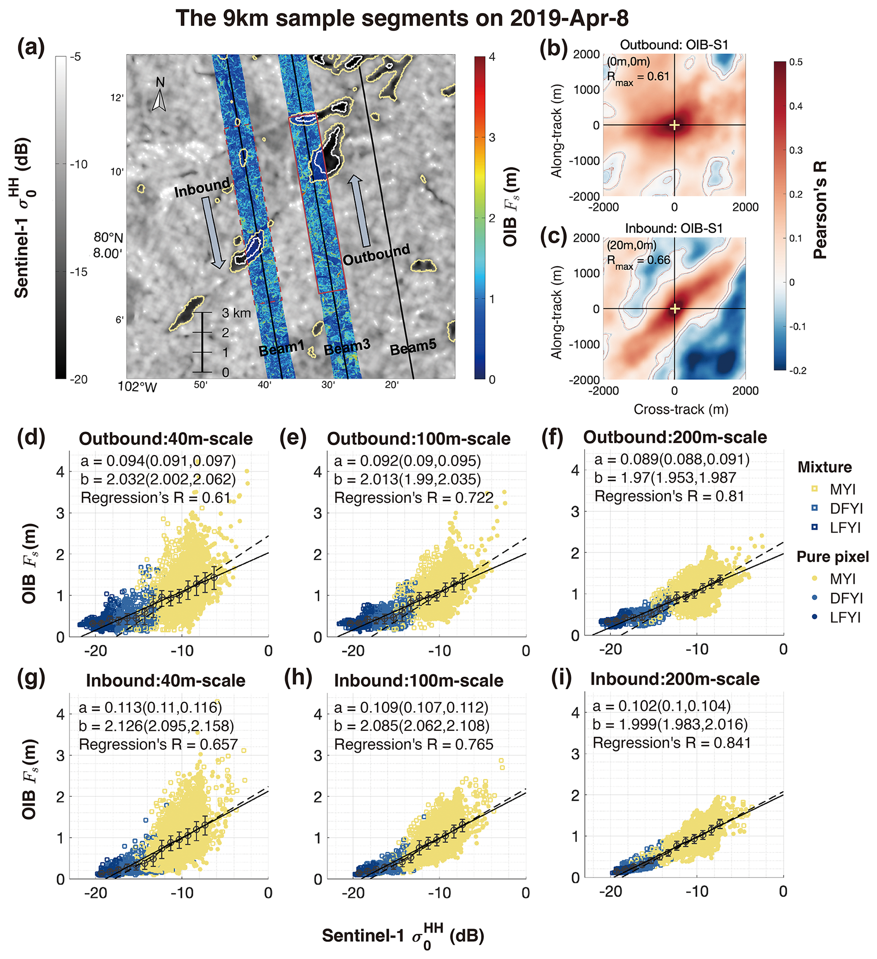
Figure 2 Total freeboard (F_s, colored) and the S1 HH backscatter (σ₀, background) over sample segments on 8 April, 2019 (a). Contour lines delineate the boundary between different sea ice types, including MYI, level FYI (LFYI) and deformed FYI (DFYI). The ICESat-2 ground tracks of the three strong beams (#1, #3 and #5) are also shown as thin black lines. Two 9 km segments on the outbound (i.e., northbound) and the inbound flights are marked out by the solid and dashed red boxes, respectively. The correlation map (Pearson's r) between σ₀ and F_s are shown with local corrections in 20 m steps in both the cross-track and the along-track direction (b, c). The yellow plus sign indicate the displacements to maximize the correlation between S1 and OIB. The scatter plots between $\stackrel{\mathrm{‾}}{F_{\mathrm{s}}}$ and σ₀ after collocation for the outbound (inbound) flights are shown in panels (d), (e) and (f) (g, h, i). Three spatial scales for computing $\stackrel{\mathrm{‾}}{F_{\mathrm{s}}}$ based on the 1 m-scale F_s maps are adopted: 40 m (S1 image resolution, (d) and (g)), 100 m (e, h), and 200 m (f, i). In panels (d) to (i), the dots are color coded according to their ice types, with the solid (dashed) lines showing the linear fitting lines of $\stackrel{\mathrm{‾}}{F_{\mathrm{s}}}=a\cdot {\mathit{\sigma }}_{\mathrm{0}}+b$ for all samples (only MYI pixels) and the fitted parameters. Also shown in each panel are the mean values of $\stackrel{\mathrm{‾}}{F_{\mathrm{s}}}$ and the IQR after binning with σ₀ (1 dB per bin).

4.1.2 Sample segments on 12 April

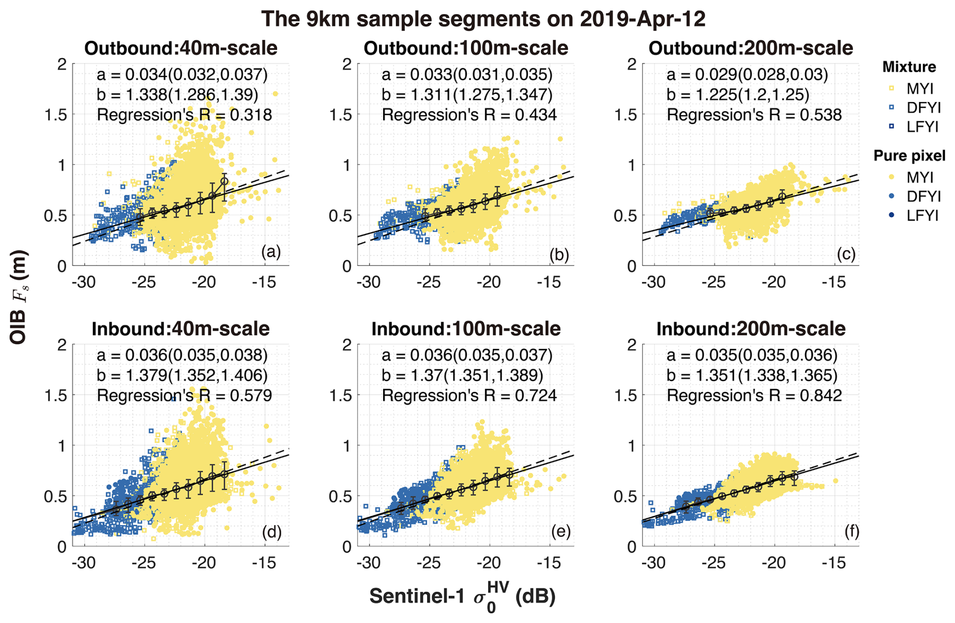
The other two 9 km sample segments are from the campaign on 12 April, shown in Fig. 3. The major differences from the sample segments on 8 April (Fig. 2) are as follows: (1) according to the OIB F_s map, the MYI is much thinner; (2) it contains higher areal fraction of FYI; and (3) the surrounding sea ice has undergone more evident drift and deformation between the observations by OIB and S1, as indicated by the OSI-455 product.

Although sea ice is generally much thinner (F_s mostly under 2 m at 1 m-scale), a statistically significant relationship is also present between $\stackrel{\mathrm{‾}}{F_{\mathrm{s}}}$ and σ₀ (Figs. 3 and C2). For comparison, we also applied a 2nd-order polynomial regression: $\stackrel{\mathrm{‾}}{F_{\mathrm{s}}}=a\cdot {\mathit{\sigma }}_{\mathrm{0}}^{\mathrm{2}}+b\cdot {\mathit{\sigma }}_{\mathrm{0}}+c$. The nonlinear model yields slightly better fitting compared to the linear regression model (see Figs. S8 and S9). For both the outbound and the inbound segments, OIB has attained sufficient sampling of MYI, but the representation of FYI is not even. Specifically, on the outbound segment, SAR pixels with ${\mathit{\sigma }}_{\mathrm{0}}^{HH}$ under 18 dB are scarce, and no level FYI is detected in the area sampled by OIB. For the inbound segment, an apparent nonlinear relationship between $\stackrel{\mathrm{‾}}{F_{\mathrm{s}}}$ and σ₀ is observed for FYI, due to the effect of ice with different levels of development. LFYI has a consistently low $\stackrel{\mathrm{‾}}{F_{\mathrm{s}}}$ around 20 cm but corresponds to σ₀ that varies over a large range of 5  dB, whereas DFYI has strongly varying $\stackrel{\mathrm{‾}}{F_{\mathrm{s}}}$ up to around 1 m over a small range of σ₀ around 2–3 dB. The linear fitting for MYI is comparable to that for all sea ice types for the inbound flight (lower panels of Fig. 3). At both 100 and 200 m-scale, the linear regressions of $\stackrel{\mathrm{‾}}{F_{\mathrm{s}}}$ to σ₀ show lower fitting slopes for MYI than for those based on all samples. The variability of F_s at 40 m scale diminishes considerably as the scale increases. In comparison, MYI always has much steeper regression lines for the sample case on 8 April across all analyzed scales (Fig. 2). This result, although potentially affected by the accuracy of the sea ice type map, highlights the importance of the sufficient sampling of various sea ice types to ensure their representation in the study of the statistical relationship.

Interestingly, for MYI which is well observed by both sample segments on 8 and 12 April, the statistical fittings between $\stackrel{\mathrm{‾}}{F_{\mathrm{s}}}$ and σ₀ show large differences. For the sample segments on 8 April, the regressions (40 m-scale) are steeper at: $\stackrel{\mathrm{‾}}{F_{\mathrm{s}}}=\mathrm{0.139}\cdot {\mathit{\sigma }}_{\mathrm{0}}+\mathrm{2.443}$ with Pearson's r=0.410 (outbound) and $\stackrel{\mathrm{‾}}{F_{\mathrm{s}}}=\mathrm{0.126}\cdot {\mathit{\sigma }}_{\mathrm{0}}+\mathrm{2.236}$ with the regression's R=0.458 (inbound). In comparison, on 12 April, the fitting slopes are shallower by about 50 %: $\stackrel{\mathrm{‾}}{F_{\mathrm{s}}}=\mathrm{0.06}\cdot {\mathit{\sigma }}_{\mathrm{0}}+\mathrm{1.338}$ with the regression's R=0.281 (outbound at 40 m-scale) and $\stackrel{\mathrm{‾}}{F_{\mathrm{s}}}=\mathrm{0.051}\cdot {\mathit{\sigma }}_{\mathrm{0}}+\mathrm{1.204}$ with the regression's R=0.263 (inbound). After binning the samples to σ₀, the regression lines (i.e., between the mean values of F_s in each σ₀ bin and σ₀'s) become flatter on 12 April: $\mathrm{mean}\left(\stackrel{\mathrm{‾}}{F_{\mathrm{s}}}\right)=\mathrm{0.051}\cdot \mathrm{mean}\left({\mathit{\sigma }}_{\mathrm{0}}\right)+\mathrm{1.244}$, compared with $\mathrm{mean}\left(\stackrel{\mathrm{‾}}{F_{\mathrm{s}}}\right)=\mathrm{0.105}\cdot \mathrm{mean}\left({\mathit{\sigma }}_{\mathrm{0}}\right)+\mathrm{2.123}$ on 8 April. The potential causes of the different fittings include both: (1) differences in C-band backscatter sensitivity to macro-scale topography due to different ice/snow properties of the two regions, and (2) different imaging configurations of the SAR images. Related issues, such as the effect of IA on the statistical relationships are further discussed in Sect. 5.1.

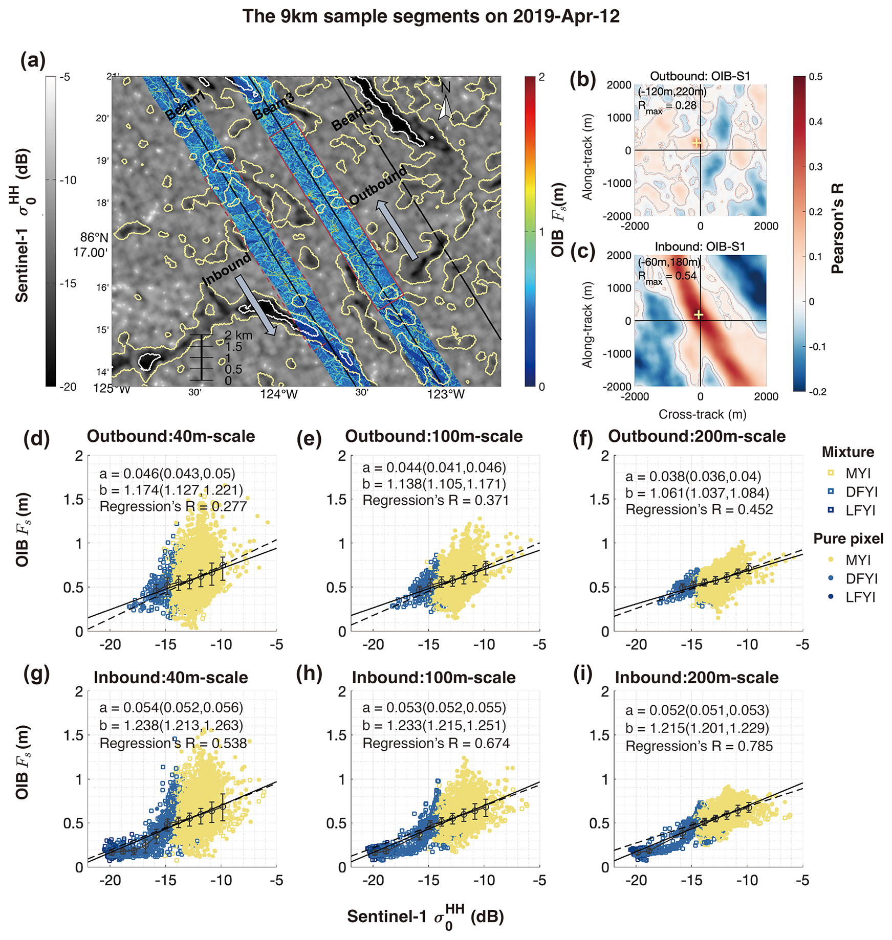
Figure 3 Same as Fig. 2, but for sample segments on 12 April.

4.2 Statistics of all segments on 8 and 12 April

For each of the 9 km OIB segment on 8 and 12 April, we generate a merged F_s map and collocate it with the SAR images on the same day. The statistical correlations are shown in Figs. 4 and 5, respectively.

On 8 April, the local corrections for collocating F_s and σ₀ are all within 40 m (Fig. 4a). The OSI-SAF drift product indicates about 100 m drift within the northern part of the OIB track, although the drift vectors are not significant given the respective product uncertainties. SAR images from the surrounding days (i.e., from 7 and 9 April, listed in Appendix B) also show little drift in the sea ice pack surveyed by the OIB campaign (details not shown). In addition, we have attained meter-scale corrections for the collocation of OIB passes (see Fig. A1). Given the relatively coarser resolution of the SAR images, we assume that sea ice drift and deformation can be ignored when collocating F_s and σ₀. The detected local corrections in Fig. 4a may not indicate actual sea ice drifts, but may be due to geolocating uncertainties, such as those induced by geometric corrections of the SAR images. The correlation between $\stackrel{\mathrm{‾}}{F_{\mathrm{s}}}$ and σ₀ at 200 m scale is statistically significant for all segments (Fig. 4b and d). After binning F_s samples to σ₀, the correlation coefficients the mean values of F_s and σ₀ within the bins are mostly over 0.9 (Fig. 4c and e).

For the OIB campaign on 12 April, statistically significant large-scale sea ice drift are observed in the surveyed region (see Fig. 5a). The lengths of the local corrections for collocating F_s and σ₀ are about 250 m. The corrections are consistent between the local segment pairs on the inbound and the outbound flights, and they also agree with the large-scale drift in terms of both direction (north-east) and magnitude. Therefore, these local corrections correspond to the actual sea ice drift between the visits by the OIB campaign and S1.

After the corrections, the correlation coefficients are higher and statistically significant for all segments (p=0.05 level). Moreover, the correlation coefficients after binning are mostly over 0.9 (Fig. 5c and e).

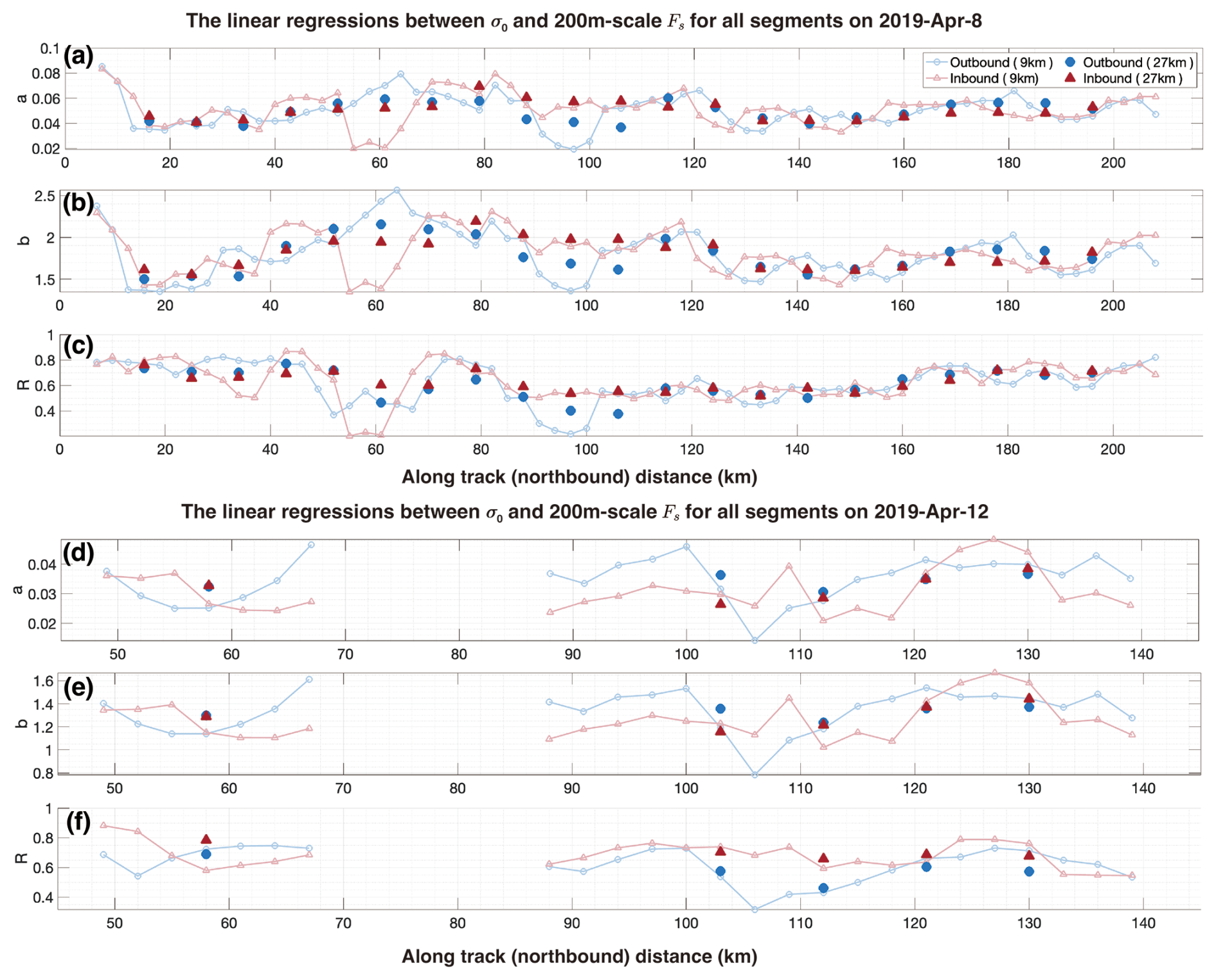
In Fig. 6 we show the linear regressions between σ₀ and 200 m-scale F_s for all segments on 8 and 12 April. The results indicate that with σ₀ and the regression relationships, we can estimate the 200 m-scale F_s with high statistical confidence (regressions' R-values over 0.3 for all 9 km segments). Furthermore, the regression parameters show significant variability among different segments, indicating the physical relationship between F_s and σ₀ varies locally. Despite this variation, the regression parameters from the inbound and outbound tracks are very similar. We further examine the relations for 27 km-long segments. As shown in Fig. 6, the regression parameters for 27 km segments are much less variant, although certain variability still exists on different parts of the flight track. Specifically, for the segments on 8 April, the variance of a (b) has decreased by 48.6 % (36.5 %) when comparing 27 km-long segments to 9 km-long segments. For the segments on 12 April, the variance of a (b) decreased even more significantly, by 76.8 % (78.7 %). Besides, the regressions' R-values are also higher for 27 km-long segments for segments on both 8 and 12 April. This implies that, small-scale inhomogeneity of the sea ice cover or errors in data co-location, which cause large variability of a's and b's in Fig. 6, are effectively attenuated at larger scales. The regression relationships in Fig. 6 can be further used for the prediction and construction of 200 m-scale F_s maps based on SAR (Figs. S10 and S11). In particular, given to the locality of the relationships, the prediction of F_s map should also be carried out adjacent to the collocating observations by SAR and altimetic scans.

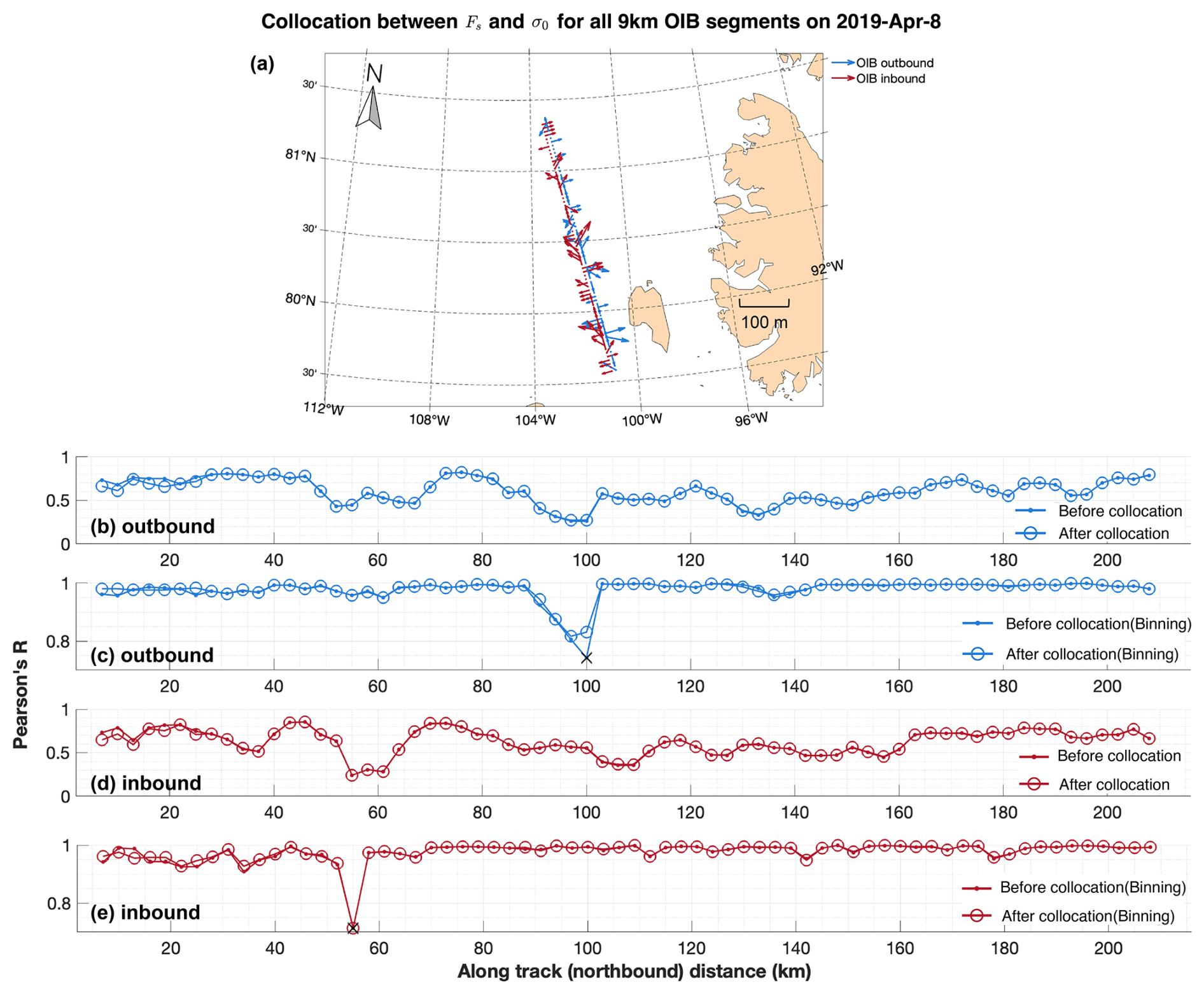
Figure 4 Statistical relationship between F_s and σ₀ for OIB segments on 8 April 2019. The local corrections to maximize the correlation between $\stackrel{\mathrm{‾}}{F_{\mathrm{s}}}$ and σ₀ are shown for all 9 km segments with valid data on the outbound flight (blue) and the inbound flight (dark red). The correlation coefficients before and after collocation are shown for the outbound (b, c) and the inbound flights (d, e) for all 9 km segments, together with those after binning. Statistically insignificant correlations are shown by crosses (×) in the lower panels (p=0.05 significance level).

Figure 5 Same as Fig. 4, but for OIB segments on 12 April 2019.

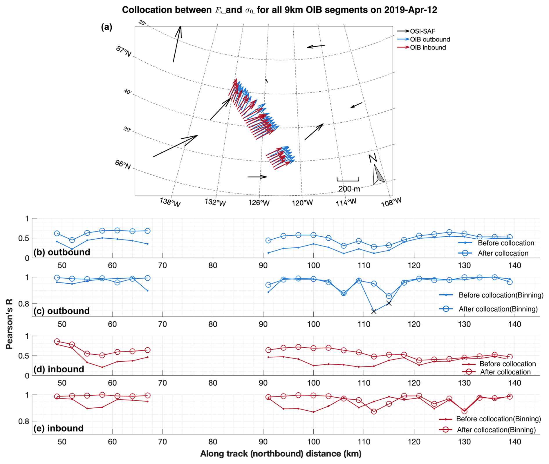
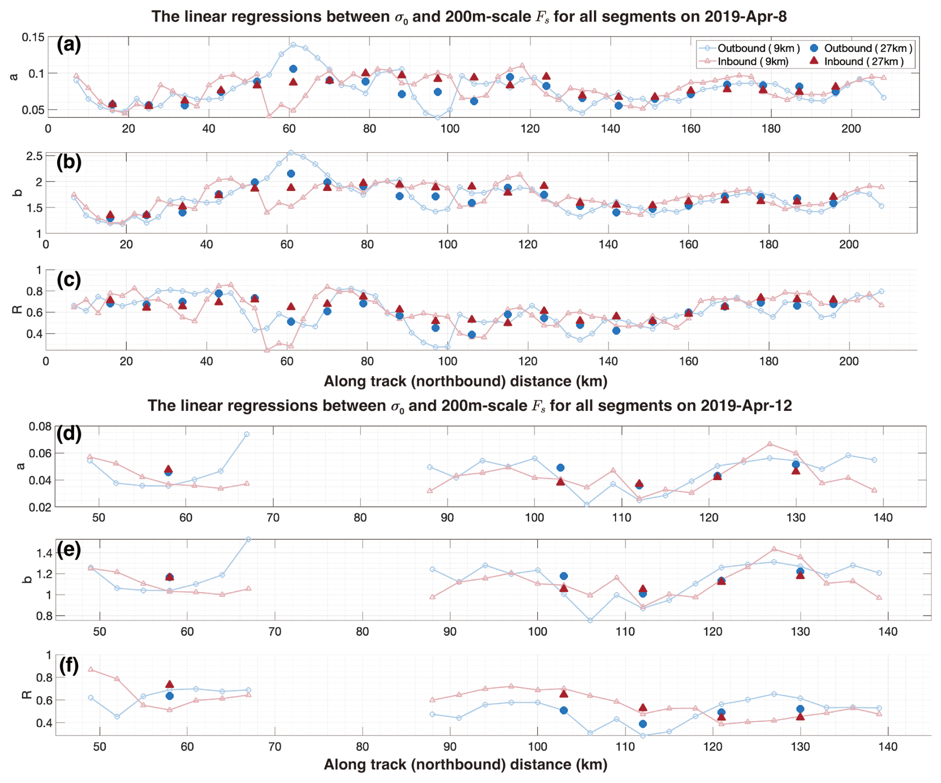
Figure 6 The linear regression from 40 m-scale σ₀ to the 200 m-scale F_s for all segments on 8 April (a, b, c) and 12 April (d, e, f): $\stackrel{\mathrm{‾}}{F_{\mathrm{s}}}=a\cdot {\mathit{\sigma }}_{\mathrm{0}}+b$. The regression's parameters, including a (a, d), b (b, e), and the R-value (c, f) are shown, respectively. Two segment lengths are adopted: 9 and 27 km.

4.3 Prediction of F_s distribution with σ₀ map

Given that the altimetric scans by OIB (and IS2) have a finer resolution than available SAR images, the regression in Sect. 4.2 is inherently limited in the spatial resolution of the predicted F_s. Moreover, although there is a significant correlation between F_s and σ₀, the variability of F_s is considerable, and no single predictor based on backscatter effectively captures this variability. Therefore, we focus on the prediction of meter-scale F_s distribution (i.e., at the full resolution of the altimeter data) with SAR images based on their collocating observations of F_s and relatively coarser σ₀ data.

4.3.1 Study of sample segments

We first study the 9 km sample segments in Sect. 4.1.1 and 4.1.2. The distributions of F_s in typical σ₀ bins of these two 9 km sample segments are shown in Figs. 7 and 8, respectively. The sample F_s distributions after binning all show the following characteristics. First, F_s follows a long-tailed, skewed distribution, which is consistent with various findings in existing studies (Xu et al., 2020; Duncan and Farrell, 2022). Second, for larger σ₀ bins, the mean value and the variability of F_s are both higher. Third, the F_s distributions are multimodal, especially for σ₀ bins that contain both FYI and MYI samples (e.g., left panels in Figs. 7 and 8).

To capture the complex shape of the F_s probability density function (PDF), we use the three-component Log-Logistic mixture distribution to fit the sample PDF in each σ₀ bin. The fitting results (i.e., Figs. 7 and 8) indicate that the different PDF modes are well captured with very low K-S distance to the sample PDF. We further carry out clustering analysis of the various components, based on the modal F_s values and the corresponding σ₀ (right panels of Figs. 7 and 8). The three clusters indicate continuous changes of the PDF parameter with respect to σ₀, and they generally show a good correspondence to these sea ice types: FYI, thin MYI and thick MYI. For example, for the sample segments on 8 April, there is prominent presence of MYI with F_s of over 3 m and σ₀ of over −5 dB (Fig. 7). This is captured by a separate Log-Logistic component which we manually categorize as the thick MYI. This could corresponds to sea ice of higher age than that of the thinner MYI which corresponds to the second component. Another example is that components with very small modal values of F_s manifest even at very large σ₀ bins (Figs. 7 and 8, lower panels). Due to the relatively coarse resolution of S1 images, thin FYI may be present in pixels with otherwise large values of both mean F_s and σ₀. These components are captured by the PDF fitting, and we further manually categorize them as FYI. It is important to note that these categorizations are introduced to interpret the fitting results, as the specific categories (FYI, thin MYI, and thick MYI) were not previously defined in our analysis. Based on the per-bin F_s fittings on the inbound sample segments, we carry out the prediction of F_s distribution on the corresponding outbound segments. Specifically, based on the observed σ₀ map on the outbound segment, we: (1) formulate the distribution of σ₀, (2) compute the F_s distribution according to the sample probability of each of the σ₀ bin, and (3) construct the overall F_s distribution on the outbound segment. For the 9 km sample segments on 8 April, the per-bin Log-Logistic mixture fittings demonstrate a high degree of accuracy in fitting the observations for both the inbound and the outbound segments, with K-S distances of 0.002 for each segment. However, the inbound and the outbound segments differ in the sample F_s distribution (Fig. 9b), primarily attributed to variations in the thickness of FYI and MYI, as well as differences in their respective proportions. Notably, the modal thickness values of both the thin MYI and the thick MYI are 0.1 m higher on the outbound segment than on the inbound segment. As a result, the predicted F_s distribution also shows lower modal F_s values (Fig. 9a). Despite the underestimation of the modal F_s, the prediction is closer to the observation, with lower K-S distance: 0.072, compared with 0.076 between the inbound and the outbound segment.

For the 9 km sample segments on 12 April, the prediction also shows lower K-S distance with the observed F_s distribution on the outbound flight (K-S distance from 0.094 to 0.074). The major improvement is due to different portions of thin FYI on the outbound and the inbound segments (see also Fig. 3). By using the σ₀ map on the outbound segment, we achieve the correct representation of thin ice in the predicted F_s distribution.

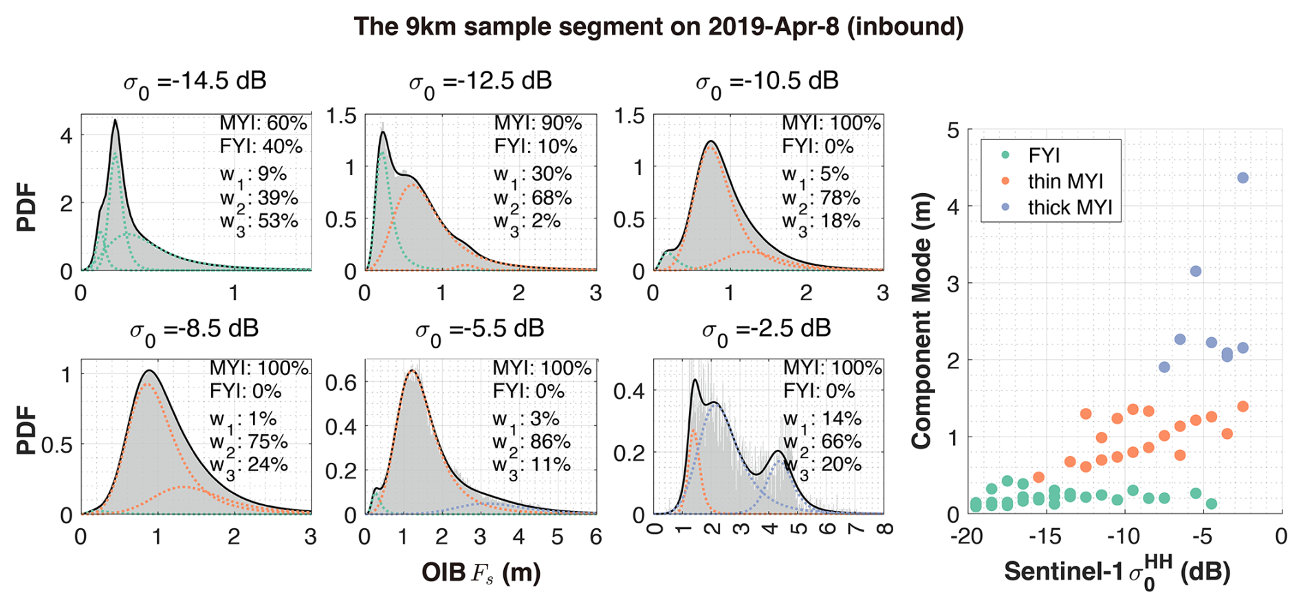
Figure 7 Distribution of 1 m-scale F_s in typical σ₀ bins of the inbound sample segment on 8 April, 2019. F_s sample PDFs, as well as the fitted three Log-Logistic mixture components are shown for typical σ₀ bins (left panels). Statistical PDF fitting (black solid line) based on the 3-component Log-Logistic mixture model in each panel, along with each of the components (colored dash lines).

Figure 8 Same as Fig. 7, but for the inbound sample segment on 12 April 2019.

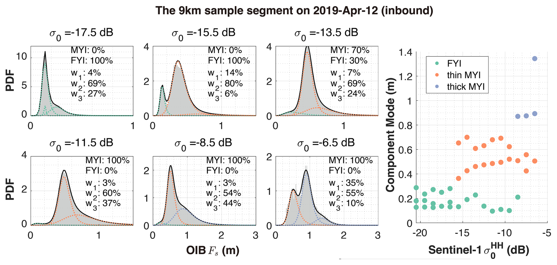
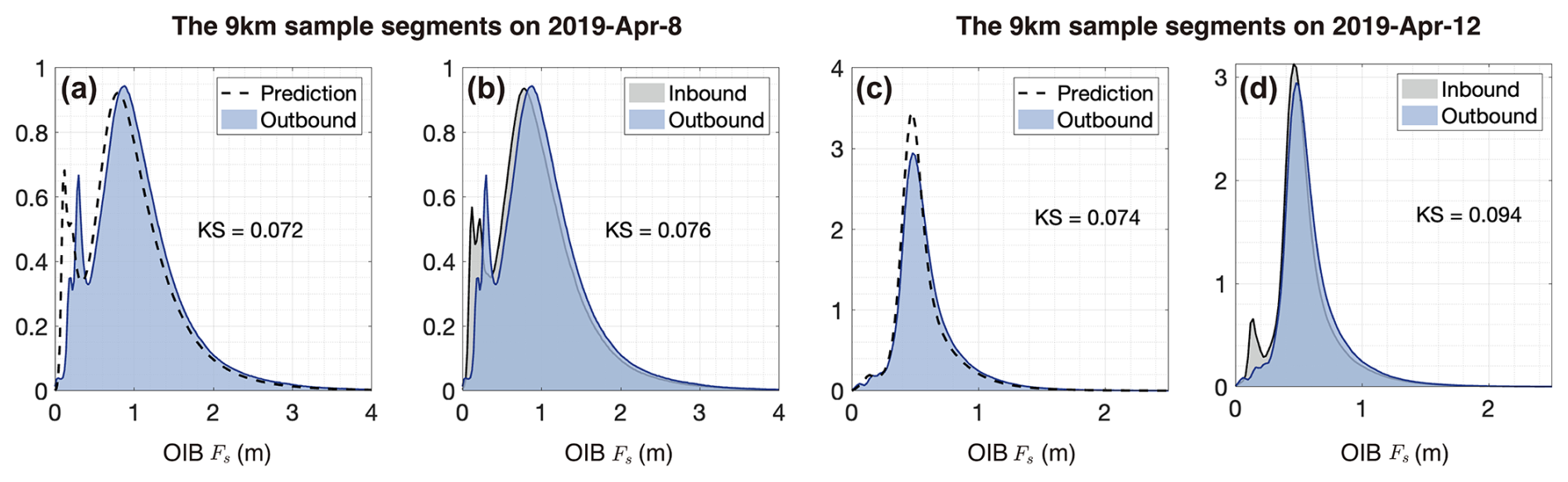
Figure 9 Statistical prediction of F_s distributions on the outbound segment with: (1) the per-σ₀ bin Log-Logistic mixture fittings on the corresponding inbound segment, and (2) the σ₀ map on the outbound segment. The observed and the predicted F_s distribution, as well as the K-S distance between the two are shown for the sample outbound segment on 8 April (a) and 12 April (c). The F_s sample distribution on the inbound and the outbound segments are also shown for comparison (b, d).

4.3.2 Validation of prediction for all segments

We carry out the prediction of 1 m-scale F_s distribution for all the 9 km outbound segments. Figure 10 shows that the predicted F_s PDF is close to the observation, with the mean K-S distance at 0.077. There is a 10 % reduction of the baseline K-S distance, which indicates that the predicted F_s distribution better matches the observations. Especially, large K-S distances are effectively attenuated with the prediction: 3 (10) out of the total 91 9 km segments show a K-S distance over 0.15 between the predicted (inbound) F_s with the outbound observations.

Moreover, there exists a significant positive correlation (Pearson's r: 0.72, p-value: $\mathrm{2.48}\times {\mathrm{10}}^{-\mathrm{16}}$) between the K-S distance sequences in Fig. 10. This indicates that when the F_s elevation is similar between the inbound and the outbound segments, the prediction is generally better. On the contrary, if the F_s distribution is more different between the two segments, the prediction also deteriorates. Therefore, in order to obtain better predictions, the observed F_s should contain sufficient sampling of different sea ice types in the range of the prediction. Representation issues for large-scale retrievals are further discussed in Sect. 5.

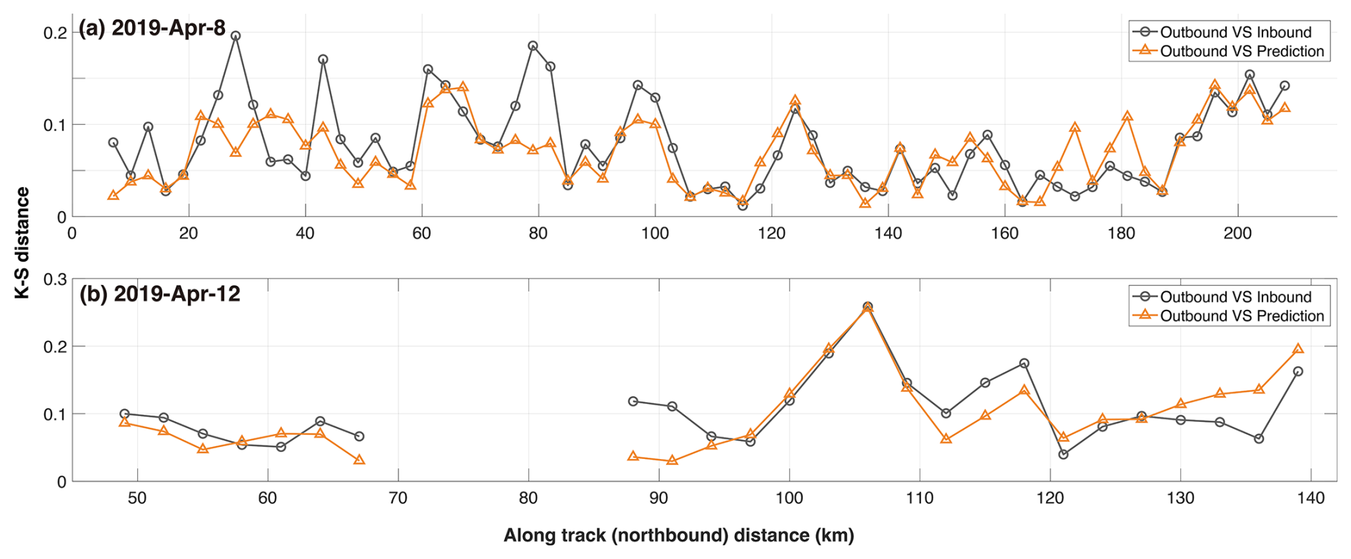
Figure 10 K-S distance between the predicted and the sample F_s distribution on all the 9 km outbound segments on 8 April (top panel) and 12 April (bottom panel). The prediction on each 9 km outbound segment is carried out with the PDF fittings on the corresponding 9 km inbound segment. The K-S distance between the inbound and the outbound sample F_s distributions are also shown.

5 Discussions and Summary

In this study we investigate the statistical relationship between sea ice freeboard and C-band microwave backscatter, by using collocated OIB observations and S1 images. Stronger SAR backscatter is observed for higher snow freeboard, which is attributed to the sensitivity of backscatter to both the sea ice type, with generally high volume scattering for MYI in winter, and ice topographic features such as ridges, with older ice having experienced stronger deformation (Krumpen et al., 2025). Moreover, the scale-dependency of this statistical relationship, along with its spatial and temporal locality, is further studied. An algorithm for predicting and extrapolating sea ice topographic measurements with SAR images is introduced that incorporates both: (1) the ICESat2 footprint size, and (2) the higher variability for larger sea ice total freeboard.

5.1 Physical mechanisms behind the statistical relationship between σ₀ and F_s

The statistical relationship between sea ice freeboard and C-band microwave backscatter is rooted in the different microwave backscatter mechanisms of various ice surface features. Thin, level ice typically exhibits low backscatter, with two primary scattering mechanisms contributing to this: surface scattering from the ice surface and volume scattering from air voids (Manninen, 1992). However, with thicker ice and larger F_s, both the backscatter and F_s variability are higher, as evidenced by the larger spread of F_s IQR in higher σ₀ bins in Fig. 2. This suggests that more complex physical mechanisms govern the C-band backscatter variations in thicker ice. In the case of older, rougher ice, the presence of thicker snow cover and more extensive ice deformation cause increased diffuse reflection and refraction of the incident radar signal (Onstott, 1992).

In addition to the wavelength-scale roughness, several other factors can also influence backscatter, such as the effective radar incidence angle, radar azimuth which are greatly affected by ridge geometry (Krumpen et al., 2025). For level ice, the effective incidence angle is relatively constant, equal to the radar incidence angle. However, for ridges, the local IA varies depending on the radar and ridge geometries, including the incident radar angle, the ridge slope, and the orientation of the ridge. Even with constant ice properties, these geometric differences alone can lead to higher surface backscatter from ridges compared to level ice (Manninen, 1992). Consequently, the radar backscatter and its IA dependency are highly dependent on the ice type and the observational geometry (Geldsetzer and Howell, 2023; Lohse et al., 2021, 2020; Guo et al., 2022). We further explore the influence of IA on the statistical relationship for the OIB track on 8 April (no evident deformation or synoptic events around 8 April). By matching SAR images from April 7th, 8th, and 9th to the OIB track on 8 April, we obtain the statistical relationships between F_s at different IAs. In general, the statistical fitting becomes steeper with decreasing IA (Fig. S4). This trend is driven by the higher (lower) sensitivity of σ₀ level (ridged) ice to changes in IA (note the weaker σ₀'s at larger IAs in Fig. S4). Therefore, when IA changes, the statistically significant relationship still holds, but IA has limited effect on this relationship than other factors, such as the localized sea ice conditions.

Furthermore, snow cover properties such as snow density and wetness can also modulate the C-band scattering signatures (Kim et al., 1984). For example, the change in snow density affects the effective wavelength of the microwave signals, therefore impacting the scattering at the snow-ice interface. Since the OIB campaigns were carried out during later winter/early spring, the snow cover is dry and therefore largely transparent to C-band signals. In order to apply the statistical prediction algorithm for other seasons (i.e., late autumn or spring), the snow conditions should be taken into account to better use the SAR measurements (Livingstone and Drinkwater, 1991).

5.2 Scale-dependency of the statistical relationship

Based on the OIB tracks on 8 and 12 April, we further explore the scale-dependent characteristics of the statistical relationship. Specifically, both F_s and σ₀ maps are coarsened to three spatial resolutions: 100, 200 and 500 m. This coarsening was achieved by calculating the average values of F_s and the S1 intensity within each coarsening grid cell at the respective resolutions, rather than coarsening the OIB F_s alone as previously shown in Sect. 4. By analyzing the coarsened σ₀ and F_s maps, we find that the relationship becomes more stable at large scales (Fig. 11). In several 9 km segments, the Pearson correlation coefficient at 500 m scale is lower than that at 40 and 200 m scale. This is likely because FYI fraction diminishes for some segments after coarsening to the 500 m scale. On the OIB tracks on 8 April, there is a special segment (∼ 55 km in along-track direction) where the Pearson correlation coefficient drops drastically across all three scales. These segments are dominated by deformed and thick ice, with a mean F_s of 1.04 m, a F_s std of 0.56 m, and MYI coverage reaching 97.3 %.

Various studies have explored the relationships between sea ice topography and microwave backscatter on different scales, ranging from SAR-related scales (Macdonald et al., 2024; Kortum et al., 2024) to scatterometry scale (Petty et al., 2017). In Macdonald et al. (2024), the Radarsat Constellation Mission (RCM, also C-band SAR) images and ICESat-2 products are used to study the relationship between sea ice roughness and backscatter over land-fast sea ice in the Canadian Arctic Archipelago. In particular, the statistical relationship based on HV-polarization is stronger, and therefore used to predict FYI roughness and the height of MYI. In our study, we also find statistically significant relationships on the HV-channel (see Appendix C). Although the HV-channel usually has a lower SNR than the HH-channel, the higher correlations with sea ice topography statistics may arise from the higher dynamic range of σ₀.

In Kortum et al. (2024) the authors explored the extrapolation of IS2 freeboard (ATL10) , allowing for a time difference of up to 24 h between S1 and IS2 measurements.

Similarly, in Macdonald et al. (2024), the HV-channel σ₀ maps are also utilized. The prediction is carried out with the pairing CDFs of F_s and σ₀, and the Pearson correlation coefficient at 400 m scale reaches 0.82. In our study, the regression model in Sect. 4.2 can also be used to predict F_s maps at similar scales. To ensure consistency with (Macdonald et al., 2024; Kortum et al., 2024), we aligned the scale of statistical relationships and performed a quantitative analysis, with results presented in Table S1 in the Supplement. However, compared to Kortum et al. (2024) and Macdonald et al. (2024), our study focuses mainly on the prediction of meter-scale F_s distributions (Sect. 4.3). In addition, we explored the effect of sea ice drift and deformation on the correlation between altimetric scans and SAR images. As shown in Sect. 4.2, third-party, large-scale drift products and local adjustments can be used to facilitate the collocation between the two. Related representation issues are further discussed in Sect. 5.3.

In Petty et al. (2017) the authors studied the statistical relationship between C-band backscatter measured by ASCAT and the variability of sea ice topography. The relationship is further used to estimate the atmospheric form drag coefficients based on backscatter maps. Although the scatterometers have relatively coarser resolution (25 km for ASCAT), the underlying mechanism of the topography-to-backscatter relationship is similar to our study. The macro-scale roughness of the sea ice cover (i.e., topography) and the sea ice type dependent surface properties affect microwave backscatter, resulting in the statistically significant relationship between the two.

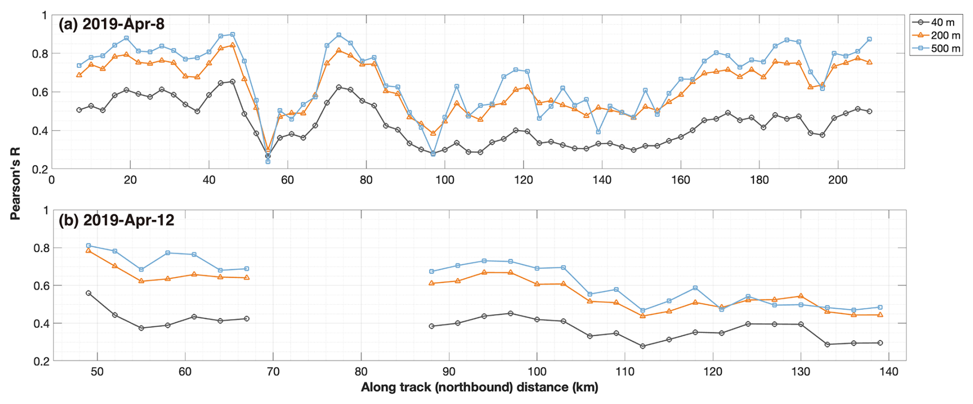
Figure 11 The statistical correlation between F_s and σ₀ at three spatial scales: 40, 200, and 500 m. The coarsening is applied to both F_s and σ₀ at these scales. The results for the OIB track on 8 and 12 April are shown in panel (a) and (b), respectively. In order to accumulate enough samples, especially at the 500 m scale, both the inbound and the outbound segments are used to compute the correlation coefficients. Note that in order to accommodate the effective resolution of σ₀ maps, in Figs. 2 and 3, we only applied spatial averaging to F_s but not to σ₀.

5.3 Spatial and temporal locality of the statistical relationship between F_s and σ₀

The statistical relationships between F_s and σ₀ in Sect. 4.1.1 and 4.1.2 are based on OIB data and SAR images acquired on the same day. Furthermore, in Sect. 4.2, we demonstrated that there is large variability in this relationship, potentially caused by differences in sea ice/snow conditions and practical factors such as different observational geometries. Therefore, the statistical relationship is spatially localized, which implies that the extrapolation of freeboard measurements (e.g., Sect. 4.3) should be carried out locally.

Furthermore, we explore the temporal transferability of this relationship, by matching SAR images collected 1 week from the OIB campaigns. Correspondingly, sea ice may undergo significant drift and deformation, as well as thermodynamic changes during a week-long interval between the OIB and SAR observations.

For the 9 km sample segments on 8 April (Sect. 4.1.1), we use SAR images from 1 and 15 April, and collocate both with the F_s map on 8 April (Fig. S5). The analysis of the drift corrections indicates that there is negligible sea ice movement between 8 and 15 April, and the statistical relationships between F_s and σ₀ are consistent (Fig. S5, lower panels). However, the maximum correlation coefficient between F_s and σ₀ is much lower at 0.4 for the SAR image on April 1st, as compared to 0.6 for 8 April (Fig. S5, upper panels). The drift corrections obtained from SAR images on 1 and 8 April confirm significant sea ice deformation, leading to suboptimal collocation between not only SAR images, but also SAR and OIB (note the scattered samples in Fig. S5b and c).

For the 9 km sample segments on 12 April (Sect. 4.1.2), SAR images from 5 and 19 April are used for a similar analysis. Between 5 and 12 April, significant sea ice drift and deformation is present for the sea ice cover around the sample segments (Fig. S6a). Correspondingly, the correlation coefficients between F_s and σ₀ also witness significant drops: from 0.28 to 0.15 for the outbound segment, and from 0.54 to 0.45 for the inbound segment. On the contrary, between 12 and 19 April, sea ice drift is evident, but very small deformation is present, as indicated by the collocation of SAR images (Fig. S6d). The correlation coefficients between F_s on 12 April and σ₀ on 19 April largely remain the same as that based on 12 April. Specifically, the coefficient is 0.27 for the outbound segment and 0.54 for the inbound segment.

Both cases indicate that the collocation between OIB and SAR deteriorates at longer time intervals, and there are corresponding drops in the statistical relationships. This is presumably caused by synoptic scale forcings that drive sea ice drift and deformations, which compromise the collocation. As indicated by both observations and modeling studies (Marsan et al., 2004; Rampal et al., 2008; Ning et al., 2024), sea ice deformation is localized, and multi-fractal both spatially and temporally. More importantly, there is strong coupling between the spatial and the temporal domain. At longer time intervals, there is lower spatial localization of sea ice deformation, which potentially complicates the collocating of SAR and altimetry scans. Furthermore, thermodynamic changes such as snowfall events, snow stratigraphic changes, as well as newly formed sea ice ridges and leads, can also greatly modulate both F_s and/or C-band backscatter(Tsai et al., 2019; Manninen, 1992). These changes are usually associated with synoptic events, which potentially co-occur with sea ice drift and deformation. In summary, there is a strong locality in the statistical relationship between F_s and σ₀. The spatial and temporal windows for collocating SAR and altimetry scans and further upscaling the freeboard measurements is an important research topic for future studies.

Figure 12 Same as Fig. 9, but for F_s on IS2 beam segments on the sample segments on 8 April (a–d) and 12 April (e–h). Since there are limited number of IS2 beam segments, the length of the sample segments is enlarged to 27 km.

5.4 On the upscaling of IS2 measurements

Compared with the 1 m-scale F_s maps from OIB, the standard sea ice elevation (ATL07) and freeboard (ATL10) products of IS2 are provided in beam segments. Since each beam segment consists of ∼ 150 aggregated photons, the nominal resolution is between 10 and 20 m in the along-track direction for the three strong beams and ∼ 11 m in the across-track direction, the laser footprint's diameter (Neumann et al., 2020). For weak beams, the beam segment resolution is even coarser by approximately 4 times. By constraining and coarsening OIB F_s maps to the footprints of IS2 strong and weak beam segments, we find that the correlation maps between F_s and S1 backscatter is in good agreement with those based on the full OIB segment (results for the sample segments shown in Fig. S7). Therefore, the collocation with S1 images can also be carried out with IS2 elevation measurements.

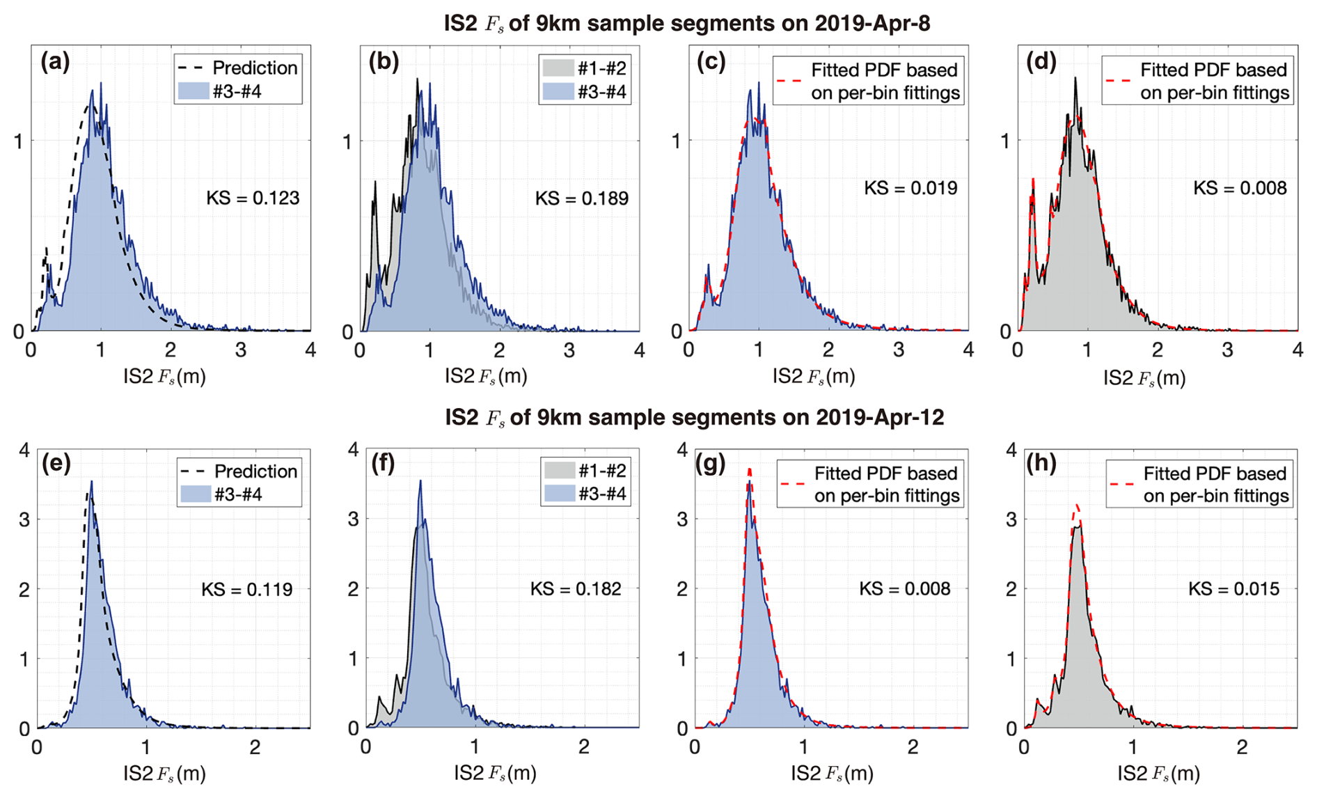
We re-apply the prediction algorithm in Sect. 4.3 to IS2 footprints of the 9 km sample segments. Specifically, the prediction is trained and validated on the IS2 beam segments on the inbound and the the outbound OIB segments, which cover the IS2 beam pairs #1–#2 and #3–#4, respectively. However, compared to the 1 m-scale OIB F_s map, the following limitations of IS2 are present: First, the IS2 beam segments are coarser, especially for the weak beams. Second, the IS2 ground coverage is much narrower at 11 m, compared with the ∼ 1.5 km width of the F_s map. As a result, on the 9 m sample segments, there is a very limited number of IS2 beam segments (i.e., $\stackrel{\mathrm{‾}}{F_{\mathrm{s}}}$ samples). Therefore, in order to accumulate enough samples for prediction, we extend the sample segments in both directions to 27 km (equivalent to the length scale used in Fig. 6).

Specifically, we follow the three-step routine for the prediction and evaluation of F_s. First, by using IS2 beam segments on the inbound segment (i.e., the #1–#2 beam pair), we bin the F_s samples to σ₀, and further carry out the PDF fitting with 3-component Log-Logistic mixture model within each σ₀ bin. Second, we predict the F_s distribution on the corresponding outbound segment, using the σ₀ observations on the IS2 footprints (i.e., the #3–#4 beam pair). Finally, we validate the prediction with the observed F_s samples.

Figure 12 shows the results for the 27 km sample segments on 8 and 12 April. Similar to the validation of the 1 m-scale F_s in Fig. 9, the prediction on IS2 footprint also yields a good match with the observed F_s distribution. In addition, the K-S distance is effectively reduced with the prediction: from 0.189 to 0.123 for the sample segment on 8 April, and from 0.182 to 0.119 for that on 12 April. Using the σ₀ map on Beams #3 and #4, we produce the F_s distribution that better matches the observation than the default F_s distribution on Beams #1 and #2. Especially, the representation of thin ice (less than 30 cm thick) has greatly improved for both cases, which is the major reason for the reduction in the K-S distance.

5.5 Outlook

Given the limitation of this case study, future work should explore the freeboard-backscatter relationship under various conditions using larger datasets. First, a more extensive coverage of sea ice types is planned, including FYI and thin ice at different stages of development. The historical records of OIB in the Arctic contain many surveys over various ice conditions especially in the western Arctic. The concurrent SAR campaigns including S1 can be used to extend the study with more complex ice types and mixtures. Second, the statistical relationship and its variability under different weather conditions need more investigation. Factors such as melt conditions and heavy snowfall could potentially alter both the microwave backscatter and the overall snow budgets. As pointed out in Sect. 5.3, we need to account for potential changes in the sea ice under synoptic events, and further obtain the optimal spatial and temporal window to derive the relationship and the upscaling of altimetry measurements.

For the upscaling of IS2 observations at basin scale, concurrent and spatially collocated SAR images should be used, such as those from S1 and the RadarSat Constellation Mission (RCM, see: MDA, 2021). Specifically, we have demonstrated both spatial and temporal locality of the derived statistical relationships. For altimetry and SAR observations that are separated by long temporal intervals, thermodynamic and dynamic processes within the ice and overlying snow can degrade the relationships between macro-scale topography and C-band backscatter. Another key factor is the spatial scale for the upscaling of IS2 measurements. In Sect. 4.3 the prediction is designed to incorporate meter-scale F_s maps. The proper temporal and spatial scales for matching SAR images and upscaling of IS2 measurements should be the subject of detailed studies in the future.

The sea ice topographic roughness and the statistical fittings are dependent on the scale of altimetric observations (Sect. 4). Beyond the OIB ATM scans (1 m-scale) and the IS2 beam segments (footprint size ∼ 11 m), various historical and future campaigns feature drastically different payload design and resolutions. For example, the nominal footprint size of ICESat is 65 m (Farrell et al., 2009), and at this scale there also exist statistically significant relationships between F_s and the C-band backscatter (Kortum et al., 2024; Macdonald et al., 2024). Besides, the concurrent SAR observations at both C- and L-bands, such as ALOS (Advanced Land Observing Satellite) and ALOS-2 (Shimada et al., 2009; Kankaku et al., 2013), can be further used for the study of the relationships and the upscaling of altimeter measurements. For ICESat, by combining with data from SAR satellite payloads such as ESA's EnviSat ASAR (Miranda et al., 2013), the upscaling of ICESat can be carried out for constructing a wider coverage record of sea ice freeboard for the period 2003–2008.

Appendix A: Processing of OIB ATM elevations

The elevations of the original ATM samples are converted into the total freeboard (or the snow freeboard, denoted F_s). For OIB flights on 8 and 12 April which were organized in a racetrack pattern(Fig. 1), we merge all OIB samples to construct a merged map of F_s for both the northbound and the southbound flight passes. Specifically, two steps are carried out, as follows.

A1 Construction of the per-pass 1 m-scale F_s map

As the first step, for each OIB pass, we converted OIB ATM samples into the F_s map which covers over 500 m across the OIB flight path. Both wide scan and the narrow scan of the OIB ATM are utilized. For a local segment along the OIB flight (e.g., 10 m in length), we first project each ATM sample under the polar stereographic projection according to its geolocation (i.e., its latitude and longitude). Then, we interpolate the samples into a 1 m-scale elevation map, using linear interpolation. Afterwards, we apply mean sea surface (MSS) geophysical height corrections to the elevation based on mean sea-surface height (DTU15 MSS model). Finally, we treat the corrected elevation as elevation anomalies, and apply the lowest elevation method to retrieve the freeboard. Specifically, the lowest 1 ‰ of elevation samples within each 10 m segment are extracted and linearly interpolated to construct the local water level (also at 1 m-scale) using the Inverse Distance Weighting (IDW) method. The final 1 m-scale F_s map is further validated with the standard 40 m-scale F_s product from IDCSI (Fig. S1).

A2 Collocation between OIB passes and the construction of the merged F_s field

We further merge the three OIB passes to form the F_s map that covers over 1.4 km across the flight path. Since the central pass and the left pass were separated by 1–2 h, and the central pass and the right pass by 3–4 h, the sea ice cover potentially had undergone drift and deformation. Therefore, we first search for corrections between each of the two pairs of OIB passes. For each 3 km segment, we maximize the correlation of the overlapping part of the F_s maps of the central and the left (or the right) pass, by adjusting the relative location of the left (or the right) pass with respect to the central pass. After the maximum correlation is attained, we record the corrections in both the along-track and the cross-track directions, and further merge the left and the right pass to the central pass, in order to form a unified F_s map. In Fig. 2a (Fig. 3a) we show the merged F_s maps for the sample segments on 8 April (12), and in Fig. S2 (Fig. S3) the correlation maps between OIB passes.

For certain segments, the central pass and the left (or right) pass do not overlap, and therefore they are not included in further analysis (especially in Fig. 5). Figures A1 and A2 show the corrections and the maximized correlation of F_s maps between OIB passes for all 3 km segments on 8 and 12 April, respectively. For 8 April, very high correlation coefficients were attained for all segments (Pearson's r all over 0.94). Besides, meter-scale corrections were required, which potentially arise from locating uncertainties. On the contrary, on 12 April, evident corrections with length over 100 m were needed to maximize the correlation, which are also consistent with the large-scale drift provided by OSI-SAF (details not shown). Therefore, we consider these corrections are associated with sea ice drifts. Evident changes of the sea ice drift at the location of 120 km along the OIB flight path is detected for both the inbound and the outbound flights, indicting the presence of sea ice deformation. Especially, the correlation coefficients for the 3 km segments also dropped to lower than 0.9 where the deformation is detected. Collocation and the resulting correlation coefficients at the scale of 500 m around the location of of the deformation further indicate that the deformation are localized (i.e., within 500 m) and present at several along-track locations (Fig. A2).

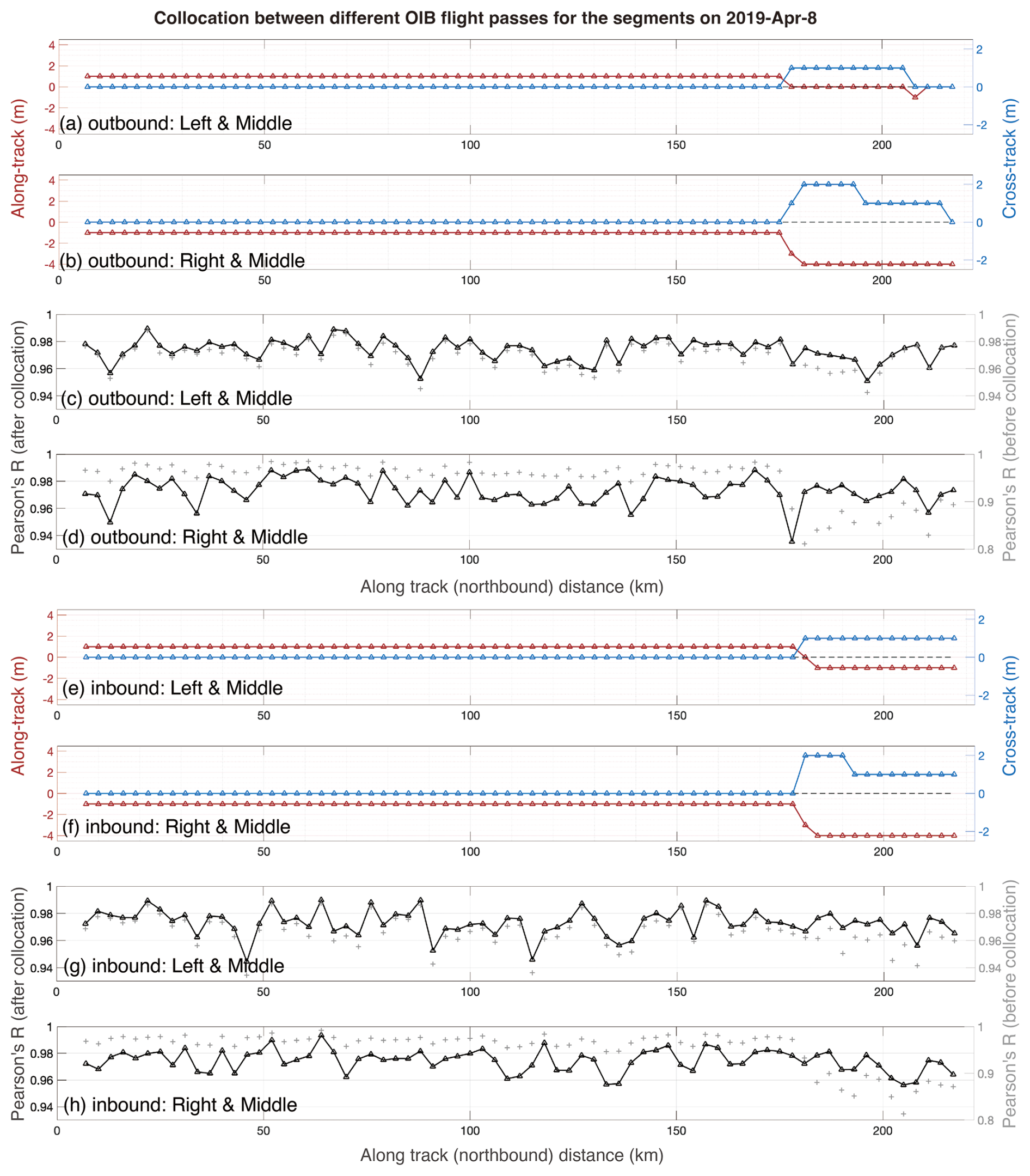
Figure A1 Collocation between different OIB flight passes on 8 April 2019. The along-track segment length is 3 km. The local corrections of the left and the right pass with respect to the middle pass for each segment on the outbound (inbound) flights is shown in panel (a) and (b) (e, f), respectively. The correlation coefficients (Pearson's r) after the collocation between the left and the middle pass and that between the right and the middle are shown in panel (c) and (d) the for the outbound flight, respectively. Similarly, panel (g) and (h) show the results for the inbound flights.

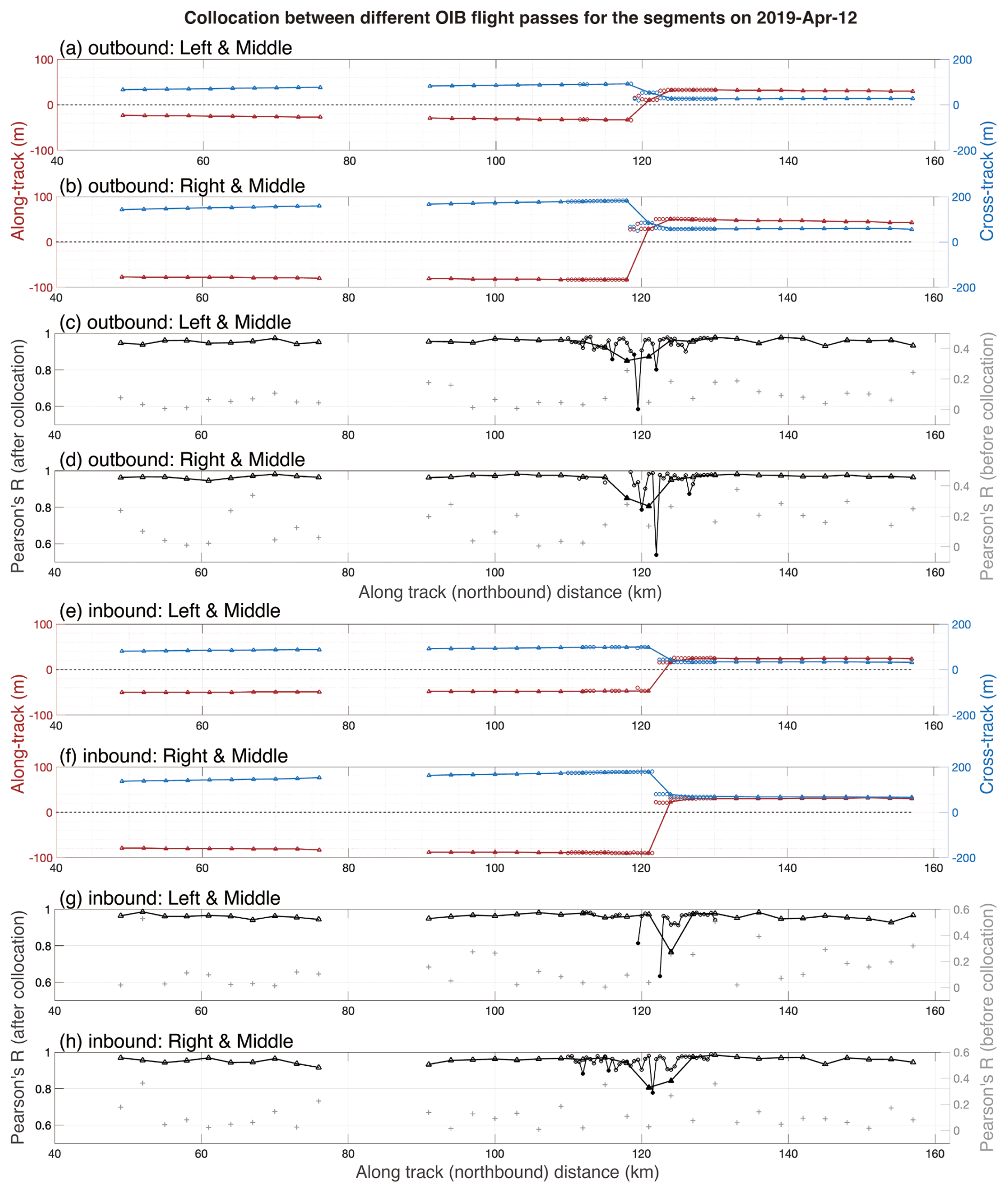
Figure A2 Same as Fig. A1, but for the OIB campaign on 12 April 2019. Correlation coefficients lower than 0.8 are marked by filled symbols in panels (c), (d), (g) and (h). For segments around the apparent deformation (at ∼ 120 km along the track), the local drift correction is further refined to 500 m in the along-track direction. The 500 m-scale drift corrections and the correlation coefficients are marked by circles and thin lines.

Appendix B: S1 EW images used for analysis for OIB campaigns

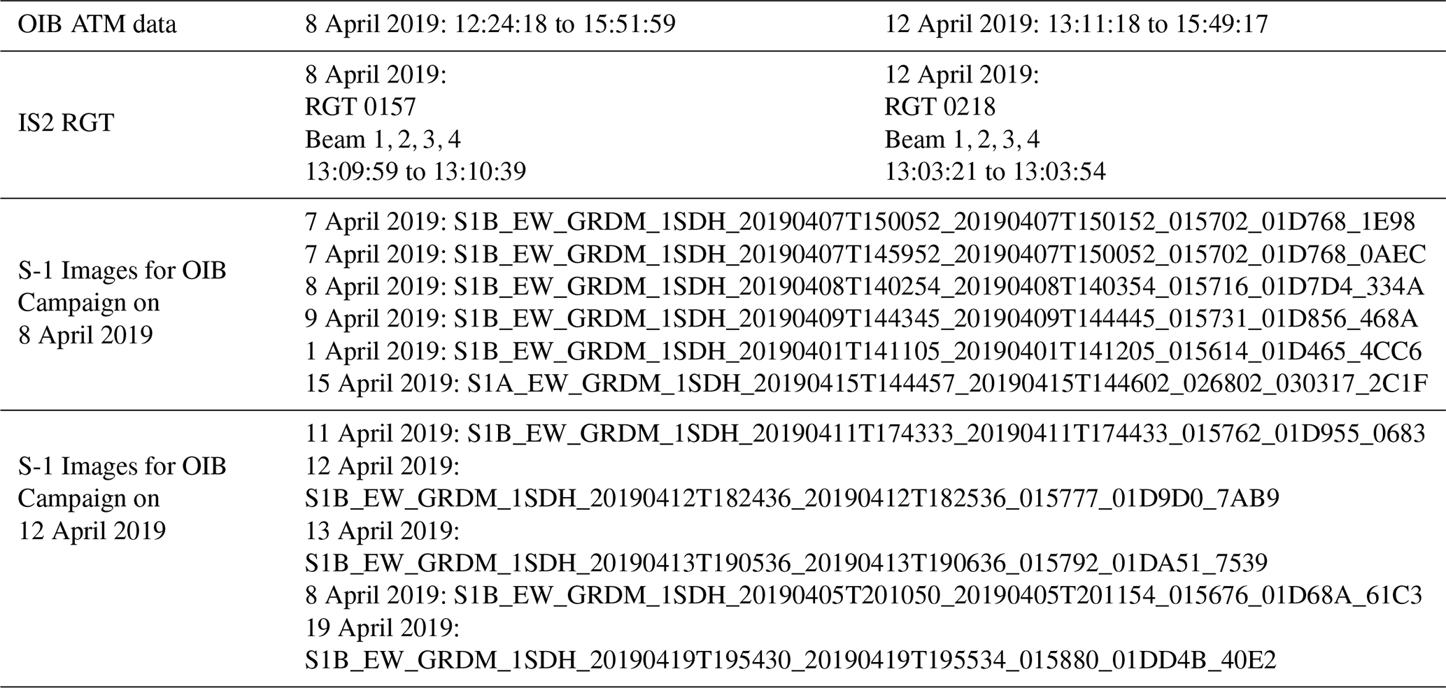
Table B1 lists the visit times of the two OIB campaigns on 8 and 12 April, as well as the matching IS2 reference ground tracks (RGTs) and Sentinel-1 EW mode images.

Table B1 OIB campaign and the corresponding S1 images. The corresponding ICESat2 ground tracks' information, including its visit times are also shown.

Appendix C: Statistical relationship between F_s and ${\mathit{\sigma }}_{\mathrm{0}}^{\mathrm{HV}}$ for the segments on 8 and 12 April

For the two pairs of sample segments on 8 and 12 April, the statistical relationship between F_s and the C-band backscatter in the HV-channel are shown below in Figs. C1 and C2. Our results show general consistency with previous studies (Macdonald et al., 2024; Kortum et al., 2024), that freeboard generally correlates slightly better with the HV-channel than with the HH-channel backscatter. The statistical relationship between freeboard and backscatter in the HV-channel for all the OIB segments are also analyzed in this section (see Fig. C3). The HV-channel backscatter is generally much weaker than the HH-channel. This is particularly evident for FYI, where HV backscatter often falls below the nominal noise floor (Segal et al., 2020). Additionally, the sub-swath artifacts are more evident in the HV-channel (i.e., abrupt transition of σ₀ across the sub-swath boundaries) for Sentinel-1 EW mode images (Lohse et al., 2021). Despite the stronger correlation observed in the HV band, the qualitative statistical relationship between freeboard and backscatter is similar when using either the HH or HV channel. Given these consideration, this work primarily concentrates on the S1 HH-channel.

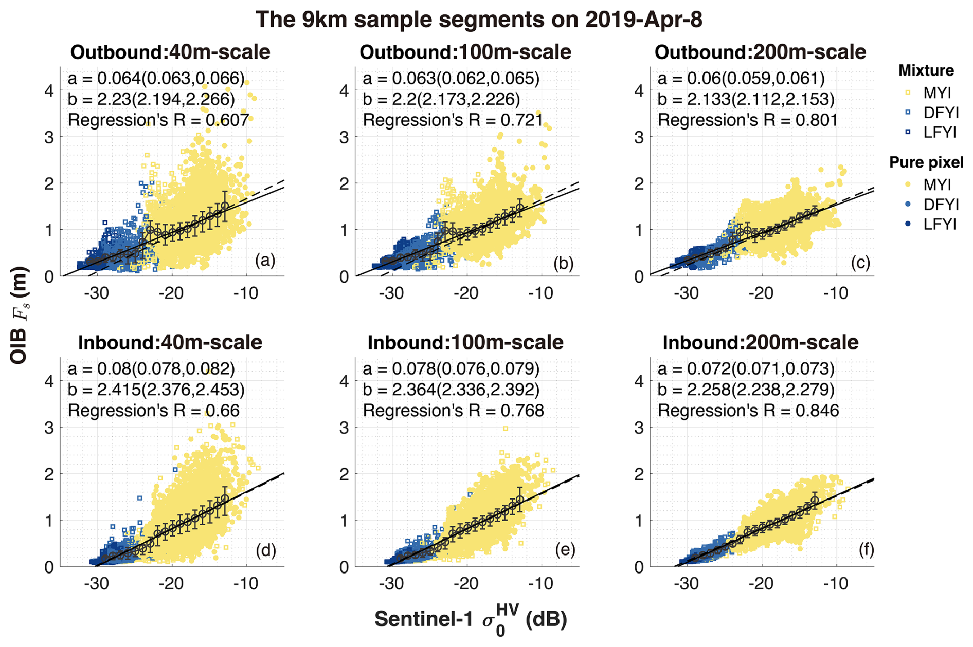
Figure C1 Scattered plot of the relationship between F_s and the Sentinel-1 C-band backscatter (σ₀) in the HV-polarization channel for the sample segments on 8 April 2019. Same as in Fig. 2, three spatial scales of F_s are adopted for matching to the 40 m-resolution σ₀ product: 40 m (left column), 100 m (middle column) and 200 m (right column).

Figure C2 Same as Fig. C1, but for the sample segments on 12 April 2019.

Figure C3 Same as Fig. 6, but for the HV-channel.