Sub-grid parameterization of iceberg drag in a coupled iceberg–ocean model

Ocean conditions in fjords play a key role in the accelerating ice mass loss of Greenland's marine-terminating glaciers. Ice mélange and icebergs have been shown to impact fjord circulation, heat and freshwater fluxes, and the submarine melting of glacier termini. Previous attempts to model icebergs largely fall into two camps: small-scale models that resolve icebergs and represent the impact of form drag and larger-scale models that parameterize sub-grid-scale icebergs but neglect iceberg drag. Here, we develop an extension of the large-scale-style iceberg package for the MIT general circulation model (MITgcm) to implement a novel, scalable parameterization to incorporate the impact of iceberg drag while also improving overall computational performance of the iceberg package by ∼ 90 %. To demonstrate our parameterization, we benchmark our method against existing iceberg-resolving models and compare it to the previous configuration of iceberg. With the inclusion of sub-grid-scale drag, our model skillfully reproduces ocean conditions and iceberg melt rates of iceberg-resolving models while reducing computational cost by orders of magnitude. When applied to a multi-month fjord-scale simulation, we find icebergs and iceberg drag have a significant impact on fjord and glacier-adjacent conditions, including cooling fjord waters and increasing circulation. We note that these effects are more moderate in the case of icebergs with drag, suggesting that studies without iceberg drag may overestimate the net impact of icebergs on the fjord system.

1 Introduction

Ice mass loss from Greenland is currently accelerating (Otosaka et al., 2023), and, for marine-terminating glaciers, this mass loss is significantly influenced by ocean and fjord conditions (Slater et al., 2020). However, significant uncertainty remains in accurately simulating ocean circulation within fjords and the precise mechanism of this influence (Morlighem et al., 2019; Slater et al., 2020; Hager et al., 2024). An important component of this system is the melt and drag from icebergs, which can modify fjord conditions through freshening, cooling, increased upwelling, and modified currents, as observed in field settings (Enderlin et al., 2016; Moon et al., 2018; Abib et al., 2024) and modeled in computational studies (Davison et al., 2020, 2022; Kajanto et al., 2023). Through these effects, icebergs can modify the near-glacier ocean conditions and thereby modulate submarine melting of the terminus (Davison et al., 2022; Hager et al., 2024). Furthermore, ice mélange, a dense rigid pack of icebergs and sea ice, can play an important role in providing buttressing stress to the glacier and can influence the calving rate (Amundson et al., 2010; Robel, 2017; Schlemm and Levermann, 2021; Amundson et al., 2025).

Icebergs and ice mélange play a particularly important role in Greenland, where many fjords are home to upwards of 10 000 icebergs at any time. In Sermilik and Ilulissat fjords in Greenland, icebergs and ice mélange have been shown to contribute over 1000 m³ s⁻¹ of freshwater flux, up to 50 % of the total freshwater flux delivered to the fjord (Enderlin et al., 2016; Moyer et al., 2019). This freshwater flux from icebergs and ice mélange melt vastly outweighs contributions from terminus melt and is comparable with subglacial discharge (Jackson and Straneo, 2016; Moon et al., 2018). Ice mélange is typically found within tens of kilometers from the glacier terminus, but iceberg melt can contribute significant freshwater flux even more than 100 km away from the glacier terminus (Moyer et al., 2019).

The melt rates of glacier fronts and icebergs are particularly sensitive to ocean velocities (Jenkins, 2011; FitzMaurice et al., 2017; Schild et al., 2021; Cenedese and Straneo, 2023; Zhao et al., 2024), and therefore it is important to realistically capture factors affecting fjord velocities. Iceberg-resolving models, which are high-resolution models that can resolve individual icebergs with grids of $\mathrm{\Delta }x,\mathrm{\Delta }y\sim \mathrm{10}$ m, have shown that icebergs impact fjord circulation through a form drag effect that can reduce velocities within an iceberg mélange by over 90 % (Hughes, 2022), even when the icebergs themselves have no skin drag (i.e., a free slip condition). This is important because the iceberg MITgcm package, a widely used parallelized numerical model for modeling iceberg thermodynamics and effects on ocean circulation, does not yet include the effect of such form drag. Thus, previous studies (Davison et al., 2020, 2022; Kajanto et al., 2023; Hager et al., 2024) have not included the impact of form drag from icebergs on ocean currents, which has been shown to be an important feedback process in the coupled iceberg–ocean system (Hughes, 2024).

Explicit representation of individual icebergs and their interaction with ocean circulation, as in Hughes (2024) and Jain et al. (2025), requires fine horizontal model resolution (10¹ m) and is thus computationally expensive to deploy in a fjord-scale model over climatically relevant timescales (months to centuries). Multi-year simulations of ice mélange have previously neglected side melting and form drag of icebergs using the shelfice MITgcm package (Wood et al., 2025). Thus, a parameterization that can accurately represent iceberg-scale drag effects in coarser-resolution fjord- and regional-scale models (10²–10³ m) is essential for capturing the influence of icebergs on ocean circulation and near-glacier properties over seasonal to multi-decadal variations in ocean, atmosphere, and glacier conditions. In this study, we develop and demonstrate a new extension of the iceberg package, which we refer to as iceberg2, which includes representation of sub-grid-scale iceberg drag effects on ocean circulation. We compare our coarse-resolution parameterization against iceberg-resolving models that specifically target the mechanical blocking and drag effect, as well as a full thermodynamic case. Additionally, we apply this new drag-enabled iceberg2 package to a multi-month fjord-scale model to demonstrate the impact of icebergs and iceberg drag on fjord dynamics for one particular idealized scenario.

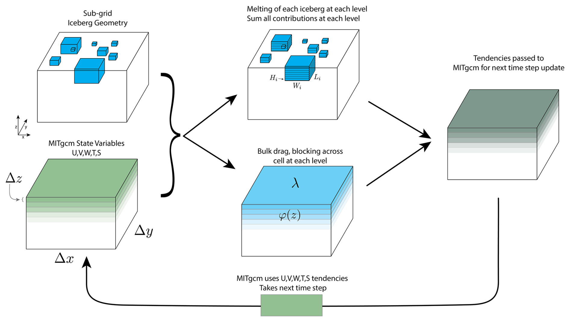
Figure 1 Simplified schematic of the iceberg2 package functionality within the MITgcm. Δx,Δy, and Δz are the resolution of the grid in MITgcm, and our schematic is drawn for a single Δx×Δy slice of the water column. Individual iceberg geometries are stored for the modeling of melt processes (upper center), while grid-averaged values of ice volume fraction φ are used to calculate blocking and drag values at each depth layer (lower center). State variable tendencies are then passed to the primary MITgcm solver, and conditions are evolved for the next time step.

2 Sub-grid parameterization of iceberg drag effect

To enable regional-scale (horizontal grid spacing >200 m) modeling, we adopt a hybrid approach to our representation of individual icebergs in our model, building on the preexisting iceberg package (Davison et al., 2020). In iceberg, the discrete geometry of each sub-grid iceberg is fully resolved for thermodynamic modeling. The rectangular dimensions (draft, width, length) of discrete icebergs within each grid (x, y location) are inputs to the model specified at initialization, allowing for an arbitrary number of icebergs per grid (x, y location) (Fig. 1). These geometries and locations are held constant in time; thus icebergs never move cells or change geometry from melting. At each time step, the melt rate is calculated using the three-equation melt parameterization (Jenkins, 2011) on each face and every depth level of every iceberg using the ambient ocean conditions within that MITgcm cell (x, y, z location). Following Cowton et al. (2015) and many others, a minimum melt velocity is imposed to parameterize the effect of ambient melt plumes. Freshwater flux, salt, and heat tendencies are summed across all icebergs within the cell (x, y, z location) and then passed to the MITgcm solver at every time step. Diagnostics of these time-varying values (freshwater flux, melt rate, and heat flux) can also be saved at each time step. Additionally, the melt parameterization is built such that it can account for the velocity of each iceberg drifting with the average ocean velocity along its entire draft, where ${\mathit{u}}_{\mathrm{drift}}={\sum }_{i\le k}\left({\mathit{u}}_i{d}_i\right)/{\sum }_{i\le k}\left(d_i\right)$. Then the velocity used for melt at every depth is ${\mathit{u}}_i^{\mathrm{melt}}={\mathit{u}}_i-{\mathit{u}}_{\mathrm{drift}}$, where u_i is the ocean velocity at layer i, d_i is the thickness of layer i, and the sum ranges over all i≤k where k is the deepest layer the iceberg reaches. In this study, we focus on icebergs fixed within a mélange and thus do not utilize this drifting option, but we keep it available for use in iceberg2.

In the development of iceberg2, we do not adjust the thermodynamic components described above, but we do adjust the implementation for faster computational efficiency (Appendix A). This results in ∼ 90 % faster computational performance in iceberg2 when considering melt alone (no drag), but the equations for calculating melt are not changed. The per-iceberg approach above is valid for thermal and freshwater contributions as icebergs contribute linearly to heat and freshwater flux, but this linear behavior does not apply for drag (Hughes, 2022). In other words, the drag exerted by a pack of icebergs is not the linear sum of the drag from each individual iceberg, since the presence of each iceberg impacts the flow conditions around other nearby icebergs.

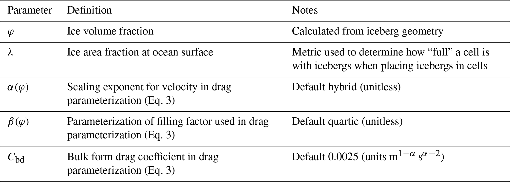
In order to add grid-scale mechanical coupling to iceberg2, the iceberg geometry is reduced to a volume fraction occupied by icebergs, φ, for each vertical layer in every cell:

$$\begin{array}{}\text{(1)}& \mathit{\phi }={\displaystyle \frac{\mathrm{1}}{\mathrm{\Delta }x\mathrm{\Delta }y\mathrm{\Delta }z}}\sum _i{W}_i\times L_i\times H_i,\end{array}$$

where the sum is over all icebergs i within a grid cell, with widths W_i and lengths L_i, and H_i is the depth the iceberg extends into the cell centered at depth z (Fig. 1). Δx and Δy are the horizontal grid spacing of the ocean model, and Δz is the vertical spacing. φ is used to calculate the parameterized bulk drag effect of all the icebergs in the cell. φ is very similar to the iceberg surface area fraction λ discussed in other studies (e.g., Hughes, 2022, 2024):

$$\begin{array}{}\text{(2)}& \mathit{\lambda }={\displaystyle \frac{\mathrm{1}}{\mathrm{\Delta }x\mathrm{\Delta }y}}\sum _i{W}_i\times L_i,\end{array}$$

where i now sums over all icebergs at the surface. λ is only defined at the surface z=0. When all icebergs in a cell extend through the full thickness of the layer centered at depth z, for example if the surface layer is thinner than the shallowest draft, φ(z)=λ. For other depths, φ is calculated by carrying out the summation in Eq. (1) at all depths and for all icebergs extending into that depth layer. As observations of icebergs at the ocean surface are the most readily available, we create our iceberg distributions based on a desired averaged iceberg surface area fraction, $\stackrel{\mathrm{‾}}{\mathit{\lambda }}$, and then calculate φ using Eq. (1) and the geometry of our iceberg distribution, which is described in more detail in Sect. 2.1.

In our model approach, there are two processes by which icebergs physically interact with the ocean: physical blocking and bulk form drag. For iceberg-resolving models, these two effects are resolved and act together by not allowing ocean flow through iceberg cells (e.g., Hughes, 2022), but for our parameterization of sub-grid-scale icebergs, we must account for each distinct process. We include the effect of physical blocking by leveraging partially filled cells with the MITgcm grid (Adcroft et al., 1997), which we detail in Appendix A. Although the previous implementation of iceberg intended to include this blocking effect, all previous studies using iceberg inadvertently had the blocking effect disabled (Davison et al., 2020, 2022; Kajanto et al., 2023; Hager et al., 2024; Slater et al., 2025). The blocking effect tends to accelerate ocean currents as they pass through the reduced open volume of partially filled cells, and, without an additional drag parameterization, blocking only results in non-physical acceleration of ocean currents passing through an ice mélange, which we discuss in Sect. 4.2.

To include the effect of form drag of many icebergs, we parameterize the bulk form drag of all icebergs within each cell at every depth layer using a form of the drag equation that can span the limits of a single iceberg to a channel-wide blockage as discussed in Hughes (2022):

$$\begin{array}{}\text{(3)}& {\mathit{\tau }}_{\mathrm{d}}=\mathit{\rho }{C}_{\mathrm{bd}}{\mathit{u}}^{\mathit{\alpha }\left(\mathit{\phi }\right)}\mathrm{\Delta }z\mathit{\beta }\left(\mathit{\phi }\right),\end{array}$$

where τ_d is the net drag stress across the layer, ρ is the density of the ocean, C_bd is a bulk form drag parameter, Δz is the vertical grid spacing of the model or model layer, and u is the ocean velocity. This drag formulation assumes icebergs are fixed in a static mélange and not freely drifting. α(φ) is the parameterized power-law scaling of velocity, and β(φ) is the parameterized filling fraction, capturing the effective frontal area of all icebergs within the cell. β captures how effectively icebergs obstruct open-flow pathways through the cell, where β=0 represents completely unobstructed flow, and β=1 means no unobstructed pathways exist. These functions, α and β, can take many forms, and we build three options for both α(φ) and β(φ) into the iceberg2 package motivated by Hughes (2022).

We build the scaling exponent for velocity in our drag parameterization with three regimes:

$$\begin{array}{}\text{(4)}& \mathit{\alpha }\left(\mathit{\phi }\right)=\left\{\begin{array}{cc}\mathrm{1}& \text{Linear}\\ \mathrm{2}& \text{Quadratic}\\ \mathrm{1}+.75\cdot (\mathrm{1}-\mathit{\phi })& \text{Hybrid (default).}\end{array}\right.\end{array}$$

The case of drag stress varying linearly with velocity best describes a full-width blockage in a stratified fluid (Klymak et al., 2010), while a quadratic relationship is more typical for an isolated obstacle, as described in Hughes (2022). When considering a large pack of obstacles in a stratified fluid, the effective power law tends to decrease from 1.75→1 as φ increases from 0→1, so we implement a “hybrid” form of α(φ) to capture the transition described in Hughes (2022) (Fig. A1a). We use this as our default form of α. We do consider other forms of α(φ) that capture the curvature of the transition, as shown in Hughes (2022), like a cubic fit, but we find results to be insensitive to this level of fitting and so defer to the simpler linear fit.

For the parameterized filling fraction, we again include three regimes:

$$\begin{array}{}\text{(5)}& \mathit{\beta }\left(\mathit{\phi }\right)=\left\{\begin{array}{cc}\mathit{\phi }& \text{Linear}\\ -(\mathit{\phi }-\mathrm{1}{)}^{\mathrm{2}}+\mathrm{1}& \text{Quadratic}\\ -(\mathit{\phi }-\mathrm{1}{)}^{\mathrm{4}}+\mathrm{1}& \text{Quartic (default).}\end{array}\right.\end{array}$$

As the cell becomes more filled with icebergs, each additional iceberg increases φ but does not necessarily increase the frontal area that contributes to drag (e.g., an iceberg immediately in the lee of another iceberg adds little additional drag). We again build in three cases, where the linear β case assumes no shadowing effect and icebergs do not block each other (i.e., the limit in which icebergs fill perfectly in the cell in the direction transverse to flow). The quadratic case follows the observed form of the fit in Hughes (2022), allowing the cell to fill rapidly at the start and saturates to full at φ=1. The case of quartic β similarly rapidly fills at low φ but now saturates to >0.95 by φ=0.6 (Fig. A1b), consistent with the observation of Hughes (2022) that after $\mathit{\phi }(z=\mathrm{0})=\mathit{\lambda }\approx \mathrm{0.6}$ the entire frontal area is typically blocked and additional filling does not increase the frontal area. We use this quartic case as our default form of β. We summarize the variables we introduce in Table 1 and plot α(φ),β(φ) in Appendix A.

We find the model is not uniquely sensitive to the exact choice of α(φ),β(φ), as tuning C_bd can significantly compensate for the particular choice of α(φ),β(φ). However, we find that our recommended choices of hybrid α(φ) and quartic β(φ) result in acceptable parameterization performance (discussed in detail below) across the entire range of $\stackrel{\mathrm{‾}}{\mathit{\lambda }},U$ we consider. We build in user control of α,β to allow flexibility when users intentionally use the model to explore specific regions of parameter space, but we caution that recalibration of C_bd is warranted for such use.

We note that our bulk form drag parameter C_bd has a similar form and value to the skin friction drag parameter used in melt parameterizations (Jenkins, 2011), but they should not be confused. The C_bd parameter here captures the independent process of bulk form drag of many icebergs and should not be confused with skin friction drag on a surface (e.g., Klymak et al., 2021). Thus, discussions of adjustment to the C_d value from Jenkins (2011), like those in Zhao et al. (2024), do not apply to the bulk form drag parameter C_bd we discuss here.

2.1 Iceberg geometries

We produce our iceberg distributions following a power-law distribution matching observations of icebergs (Enderlin et al., 2016; Sulak et al., 2017), in which the relative number of icebergs (N) depends on the horizontal area of the iceberg (A) and so varies according to $N\sim A^{-\mathrm{1.9}}$. We generate these icebergs by randomly generating iceberg areas from this power-law distribution until we are sufficiently close to the desired total horizontal area of icebergs (within 0.5 %) and then randomly distribute those icebergs across iceberg-containing cells within our domain. In this distribution process, some cells become slightly overfull (i.e., above the average iceberg surface area fraction $\stackrel{\mathrm{‾}}{\mathit{\lambda }}$) as this captures some of the variability of the randomly placed icebergs in iceberg-resolving models, as well as the non-uniform distributions of naturally occurring icebergs.

We set the draft of every iceberg D_i as a function of its horizontal area A_i:

$$\begin{array}{}\text{(6)}& D_i=a{A}_i^{b-\mathrm{1}},\end{array}$$

where a,b are normally distributed variables with means of 6 and 0.3 and standard deviations of 1.22 and 0.016 respectively (Sulak et al., 2017). Our results are particularly sensitive to statistics of the draft of our icebergs, so we encourage care in future studies in setting iceberg draft. In particular, setting an abrupt Heaviside-style minimum draft results in large numbers of icebergs that terminate in one particular depth cell, and this leads to unrealistically high freshwater flux and vertical shear values for this layer. For this reason, we find it important to set draft as a randomly varying function of iceberg horizontal area. Due to the random distribution of our iceberg drafts, any stated minimum or maximum values are only restrictions on the mean of the distribution (Eq. 6), and the actual extreme values will likely extend beyond these values.

Table 1 Summary of parameter definitions and defaults used in this study.

3 Application to ocean modeling in the MITgcm

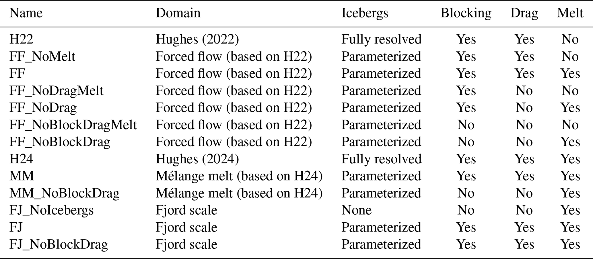
We benchmark the new drag and blocking components of the iceberg2 package against Hughes (2022), an iceberg-resolving ocean model in the MITgcm that omits the effect of melt, across a range of average iceberg surface area fractions, $\stackrel{\mathrm{‾}}{\mathit{\lambda }}$, and forcing current speeds, U. This initial benchmarking is done with iceberg melt disabled, following Hughes (2022). We also use the same geometry to consider the impact of blocking alone (no drag) and the addition of iceberg melt. The implementation of these configurations is detailed in Appendix A. We then benchmark the full thermomechanical case of melting icebergs with and without iceberg drag against the thermomechanically coupled iceberg-resolving MITgcm study from Hughes (2024). Finally, we run a fjord-scale domain over several months to demonstrate the functionality and scalability of our iceberg parameterization.

Hughes (2022)Hughes (2024)

Table 2 Full list of cases, model domains, and physics resolved in each case discussed.

3.1 Model domains

We set up our forced-flow domain following the configuration described by Hughes (2022) for a 2.4 km × 2.4 km mélange pack floating in a rectangular channel with vertical walls that is 32 km long, 2.4 km wide, and 600 m deep (Fig. 2a), subject to a forcing current that varies vertically (Fig. 2b).

$$\begin{array}{}\text{(7)}& U\left(z\right)=U\cos \left({\displaystyle \frac{\mathit{\pi }z}{\mathrm{600}}}\right)\end{array}$$

The fjord is initialized with a uniform salinity and linearly varying temperature (Fig. 2b) and with a linear equation of state. This creates a linear density profile such that the Brunt–Väisälä frequency, $N=\mathrm{5.2}\times {\mathrm{10}}^{-\mathrm{3}}$ s⁻¹, is comparable to average values for Greenlandic fjords (e.g., Sanchez et al., 2023). In Hughes (2022), this density gradient is produced by a temperature gradient alone to allow the salt solver in MITgcm to be disabled, which increases computational efficiency. To produce a realistic density gradient, Hughes (2022) set the temperature field to nonphysical values, with temperatures as low as −8.3 °C for liquid water. We follow this configuration to match that of Hughes (2022) for this benchmarking exercise; however we note that the equivalent density gradient from a more physical salt gradient (0 °C, 34 PSU at the surface and 36.24 PSU at 600 m) was also tested and produces identical results for model runs with no iceberg melt. We use a coarser spatial resolution of $\mathrm{\Delta }x=\mathrm{\Delta }y=\mathrm{200}$ m (compared to 10 m in Hughes, 2022) and a slightly coarser vertical resolution with 50 layers, Nr=50 (compared to 64). As a result of this coarser resolution, Courant–Friedrichs–Lewy (CFL) constraints are weaker, and we can use a longer time step of 15–25 s (instead of 1–2 s). We enable implicit viscosity and diffusivity using a 3D Smagorinsky scheme (Smagorinsky, 1963), with background values of vertical and horizontal viscosity set to 10⁻⁴ and 10⁻³ m² s⁻¹ respectively and background diffusivity of 10⁻⁵ m² s⁻¹.

We spin up the forced-flow model using the same 8 h spin-up process as in Hughes (2022): using a modified rbcs package, in the first 4 h the entire domain is subject to a restoring force, followed by a 4 h linear ramp-down in restoring force strength, and then for the remaining model run the restoring force is only present in 8 km sponge regions at the east and west boundaries of our domain. Sidewalls and the bottom are set to a free slip kinematic boundary condition. Given the reduced computational needs of our model, we run all simulations for 3 d (compared to 36 h in Hughes, 2022), which we find further reduces transient effects in the results but does not significantly impact our findings.

We set a minimum iceberg width of 40 m and maximum depth of ∼ 140 m to match the distribution of icebergs in Hughes (2022). Although we use very similar statistics in our generation and placement of icebergs, our iceberg fields are not identical, so some variability in our results may be explained by random differences in iceberg distributions. To model the melt of icebergs and ice mélange, we follow the “high-melt” case of Hughes (2024) using the three-equation melt parameterization (Jenkins, 2011), specifying ${\mathit{\lambda }}_{\mathrm{1}}=-\mathrm{5.75}\times {\mathrm{10}}^{-\mathrm{2}}$ °C, ${\mathit{\lambda }}_{\mathrm{2}}=\mathrm{9.01}\times {\mathrm{10}}^{-\mathrm{2}}$ °C, ${\mathit{\lambda }}_{\mathrm{3}}=\mathrm{7.61}\times {\mathrm{10}}^{-\mathrm{4}}$ °C m⁻¹, ${\mathit{\gamma }}_t=\mathrm{4.4}\times {\mathrm{10}}^{-\mathrm{3}}$, ${\mathit{\gamma }}_s=\mathrm{1.24}\times {\mathrm{10}}^{-\mathrm{4}}$, and the minimum velocity of u_min=0.04 m s⁻¹. We follow Hughes (2024) in our notation, using γ_t,s to directly represent the Stanton number (St), instead of using formulations involving Γ_t,s, but note that these are related terms with ${\mathit{\gamma }}_{t,s}=\sqrt{C_{\mathrm{d}}}{\mathrm{\Gamma }}_{t,s}=\mathit{St}$.

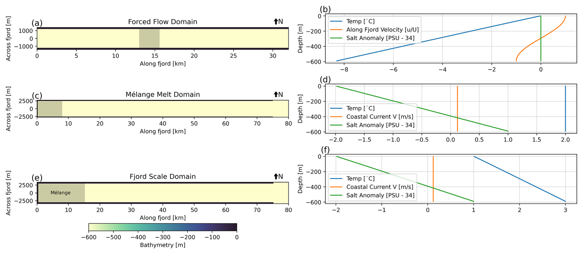
Figure 2 Model domains and boundary conditions for our three model configurations. (a, b) Bathymetry and forcing conditions for the forced-flow domain following Hughes (2022). (c, d) Bathymetry and initial/boundary conditions for the mélange melt domain following Hughes (2024). (e, f) Bathymetry and initial/boundary conditions for our fjord-scale domain. In (a), (c), and (e), gray shading indicates the location of the ice mélange, and black regions are the wall boundaries of bathymetry of 0.

For our second benchmark, the mélange melt domain, we follow the configuration described by Hughes (2024) for a 8 km × 5 km mélange pack of average surface ice fraction, $\stackrel{\mathrm{‾}}{\mathit{\lambda }}=\mathrm{0.10}$, in a 600 m deep, vertically walled channel. The west end of the channel is abutted by a glacier terminus, where ambient melt is modeled by the iceplume package (Cowton et al., 2015). We again use a coarser spacial resolution of $\mathrm{\Delta }x=\mathrm{\Delta }y=\mathrm{200}$ m (compared to 10 m in Hughes, 2024) and a slightly coarser vertical resolution Nr=50 compared to 64. The walls are vertical with a free slip kinematic boundary condition. We extend our domain 80 km to the east, longer than the 35 km in Hughes (2024) to reduce the effect of boundary conditions. We impose an along-coast current in the eastern 5 km of our domain, where an open boundary is implemented with the open boundary conditions for the regional model package (obcs). The mélange floats in a uniform 2 °C ocean with a linear vertical salinity gradient (Fig. 2c, d), and we now use a non-linear equation of state (Jackett and Mcdougall, 1995). Following Hughes (2024), the iceberg maximum draft is set to ∼ 200 m. We run this simulation for 7 d, with no other external forcing. Apart from this, the model settings are the same as in the forced-flow domain.

For our final fjord-scale domain, we use a 5 km wide, vertically walled 600 m deep, 80 km long fjord with a glacier terminus on the western end. The mélange is 15 km long and 5 km wide and has linearly decreasing $\stackrel{\mathrm{‾}}{\mathit{\lambda }}=\mathrm{0.60}$–0.01 from 0 to 15 km along the fjord. We initialize the fjord (Fig. 2e, f) with linear temperature and salinity profiles, which are forced at the 5 km wide eastern open boundary where there is again an along-coast current. We allow for ambient melt across the glacier terminus and force the system with a subglacial discharge through a half-conical plume, initialized with 500 m³ s⁻¹ of freshwater at the bottom of the glacier ($z=-\mathrm{600}$ and x=0 m) implemented with iceplume (Cowton et al., 2015). We use a coarser horizontal resolution than in previous simulations of $\mathrm{\Delta }x=\mathrm{\Delta }y=\mathrm{400}$ m and simulate 200 d of melt. Apart from this, the model settings are the same as in the mélange melt domain.

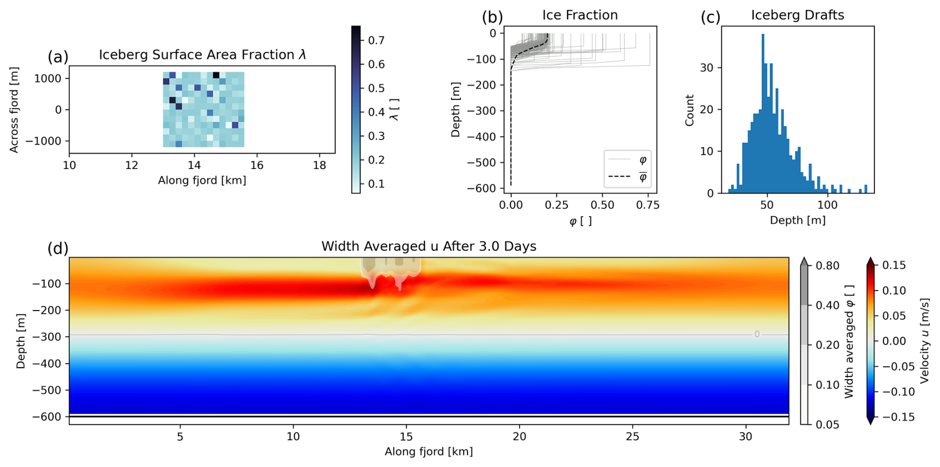
Figure 3 The configuration of our model domain for the $\stackrel{\mathrm{‾}}{\mathit{\lambda }}=\mathrm{0.20}$, U=0.12 m s⁻¹ case. (a) Distribution of λ across the mélange pack. (b) Depth variance of φ. Light gray shows φ(z) of every cell containing icebergs, and the dashed black line shows the average φ over the entire mélange area, $\stackrel{\mathrm{‾}}{\mathit{\phi }}\left(z\right)$. (c) Histogram of iceberg drafts. (d) Width-averaged velocity of our model domain at the end of the simulation. Cells are shaded with the width-averaged value of φ to illustrate the location of the mélange pack.

4 Forced-flow domain results

We test the correspondence between our parameterized model and the iceberg-resolving model of Hughes (2022) by exploring a range of iceberg surface area fraction $\stackrel{\mathrm{‾}}{\mathit{\lambda }}$ and forcing current velocity U. Hughes (2022) does not consider melt effects, so we implement FF_NoMelt-style model runs for comparison. We use the free parameter C_bd to tune these model runs but select one constant value of C_bd=0.0025 across all runs shown here (our tuning process is described in Appendix B). We find that this value of C_bd results in a good fit across all $\stackrel{\mathrm{‾}}{\mathit{\lambda }},U$ values considered. We note that for a given range of $\stackrel{\mathrm{‾}}{\mathit{\lambda }},U$, we expect C_bd to depend on the choice of α(φ),β(φ), but we do not explore that region of parameter space here.

The primary metric of comparison between our parameterized model and the iceberg-resolving model is the mean modeled ocean velocity within the mélange pack, as this is the first-order control on iceberg melt rates. To calculate this velocity, we average over the non-iceberg volume of each cell across the entire mélange pack and extract the velocity above 300 m depth, as shown in Fig. 4. For each set of $\stackrel{\mathrm{‾}}{\mathit{\lambda }}$ and U values, we plot the mean velocity within the ice mélange, normalized by maximum driving velocity (i.e., $\frac{u\left(z\right)}{U}$), for both our parameterized model (solid line) and the iceberg-resolving model of Hughes (2022) (dashed line). The normalized driving velocity, $\frac{U\left(z\right)}{U}$, is plotted as a dotted black line. We also plot the median and 90th percentile for iceberg draft in the $\stackrel{\mathrm{‾}}{\mathit{\lambda }}=\mathrm{0.2}$ case with dashed red lines.

Our coarse-resolution model replicates the important features of the iceberg-resolving model. In both models, the presence of the mélange causes a significant decrease in velocity near the surface compared to the forcing velocity at this depth. While iceberg drag slows velocity near the surface, there is an enhancement of flow in both models below the deeper drafts (90th percentile) of the mélange. This large-scale behavior is a response to the ice mélange acting as a permeable channel-wide blockage: forcing a portion of flow under the effective depth of the mélange and another portion flowing through the ice mélange via tortuous paths at a reduced speed.

To quantify the difference between our model and the iceberg-resolving model of Hughes (2022), we plot the relative residual

$$\begin{array}{}\text{(8)}& \mathit{ϵ}\left(z\right)={\displaystyle \frac{u\left(z\right)-u^H\left(z\right)}{U\left(z\right)}}\end{array}$$

and show the root mean squared error (RMSE; over the upper 100 m and upper 275 m of the domain) in the legend of Fig. 4c and d:

$$\begin{array}{}\text{(9)}& {\mathrm{RMSE}}_{\mathrm{100}}=\sqrt{\sum _{i=\mathrm{1}}^{N_{\mathrm{100}}}{\displaystyle \frac{\mathit{ϵ}(z_i{)}^{\mathrm{2}}}{N_{\mathrm{100}}}}},{\mathrm{RMSE}}_{\mathrm{275}}=\sqrt{\sum _{i=\mathrm{1}}^{N_{\mathrm{275}}}{\displaystyle \frac{\mathit{ϵ}(z_i{)}^{\mathrm{2}}}{N_{\mathrm{275}}}}},\end{array}$$

where u^H(z) is the velocity from the iceberg-resolving study of Hughes (2022), z_i is the depth of layer i, U(z) is the driving velocity (Eq. 7), and N₁₀₀,N₂₇₅ is the number of layers above 100 and 275 m depths respectively. We focus our attention on the upper 100 m (RMSE₁₀₀) as this is the region representing more than 90 % of all iceberg drafts and where the vast majority of melt would occur. We also report RMSE₂₇₅ for those more concerned with ocean currents generically. We omit residuals near $z=-\mathrm{300}$ m since the forcing velocity U(z) goes to 0 at this depth, and thus the denominator goes to 0 in the calculation of relative residuals. Below $z=-\mathrm{300}$ m, the flow is virtually unaffected by the mélange (Fig. 3d), and thus we focus our analysis, like Hughes (2022), on the upper 300 m results. Across the entire $\stackrel{\mathrm{‾}}{\mathit{\lambda }},U$ parameter space that we explore, we generally find good correspondence to Hughes (2022). Specifically, we find that velocity residuals within the upper 50 m of the water column (median iceberg draft) are always less than 15 % of driving velocity compared to Hughes (2022). The total root mean squared error for our model is 6 % of driving velocity for the upper 100 m of ocean (RMSE₁₀₀) and 9 % of driving velocity for the upper 275 m of ocean (RMSE₂₇₅, Appendix B).

The sinusoidal profile of velocity as a function of depth is expected for blocked flow in a stratified medium (Klymak et al., 2010), and the sinusoidal nature of our residuals arises from a mismatch in the wavelength of this effect in our model. Above the median iceberg draft, there is a region of positive residual velocities (faster velocities) across most runs at ∼ 25 m depth. In contrast, within 15 m, the surface residuals are often negative ($\mathit{ϵ}\sim -\mathrm{0.05}$), though this trend is not true at the bounds of our parameter sweep (high λ, high and low U). Below the median draft of the mélange, residuals are generally negative (slower velocities) until below the deeper drafts of ∼ 100 m. Again, this trend does not hold for the most extreme values of our parameter sweep. The RMSE₂₇₅ values are generally higher than RMSE₁₀₀ as the magnitude of the velocity maximum underneath the mélange (100–150 m in Fig. 4a, b) is generally not as well resolved by our parameterization compared to shallower waters (relative residual maximums in c and d between 100–150 m).

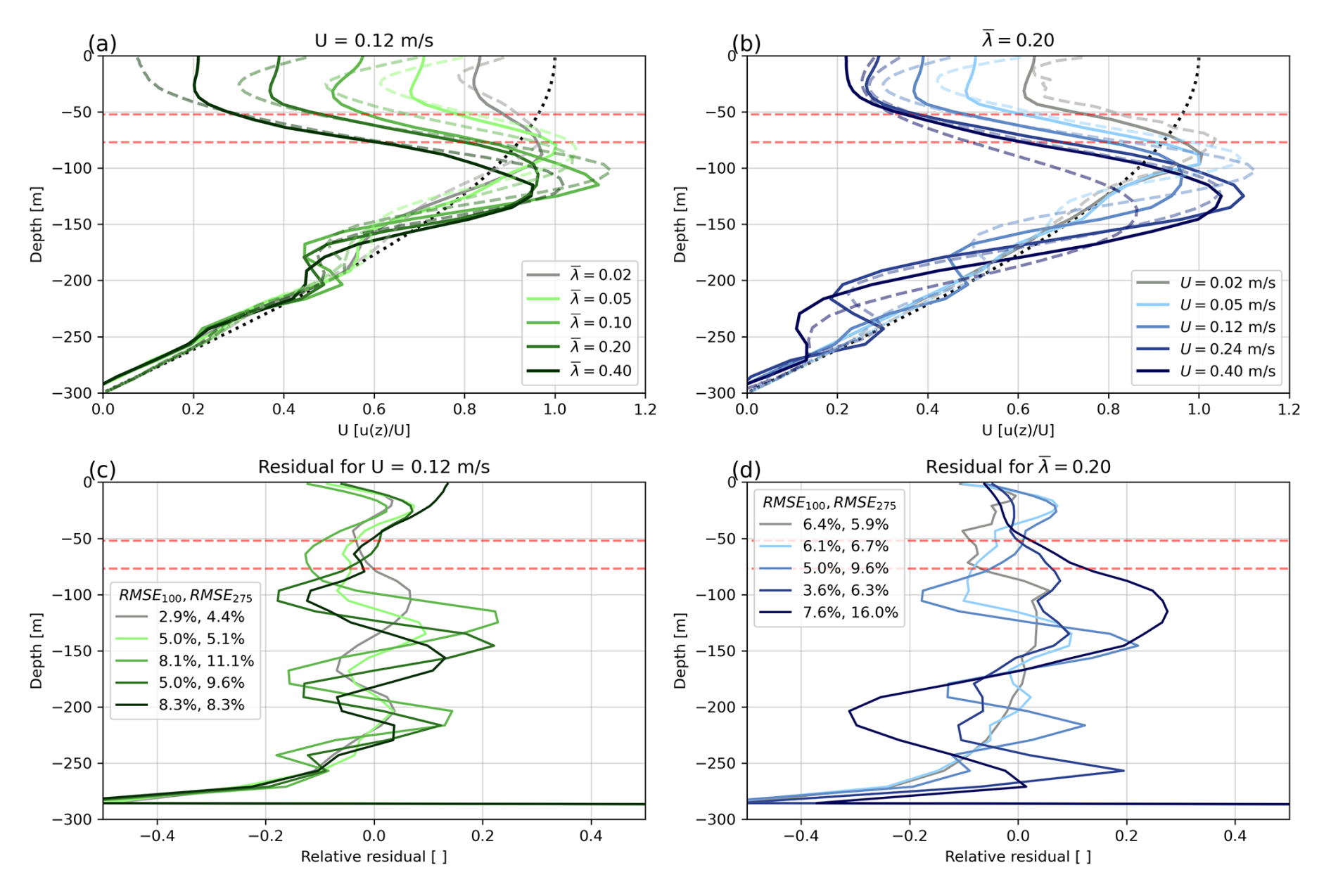
Figure 4 Along-fjord ocean velocity averaged over the mélange pack for a range of $\stackrel{\mathrm{‾}}{\mathit{\lambda }}$ in (a) and U in (b). Solid lines are this study; dashed lines are Hughes (2022) for the same conditions. The dotted black line is the driving velocity. Velocities are normalized by the driving velocity (U). Dashed red lines are the median and 90th percentile of iceberg draft for λ=0.2. Panels (c) and (d) show the relative residual ϵ (Eq. 8) for (a) and (b) respectively and list the RMSE₁₀₀ and RMSE₂₇₅ for each case in the legend. Panels (c) and (d) share the color scale of (a) and (b) respectively.

4.1 Sensitivity to model resolution

The utility of the parameterization we develop here is to capture the effects of a sub-grid-scale process in a way that is computationally efficient for use in larger-scale modeling. Therefore, understanding how our parameterization error varies with grid resolution is crucial for its careful application to larger-scale models. To investigate this effect, we repeat the $U=\mathrm{0.12},\stackrel{\mathrm{‾}}{\mathit{\lambda }}=\mathrm{0.20}$ case for a range of grid resolutions. We vary Δx from 100 to 2400 m while fixing Nr=50, and we vary Nr from 10 to 120 while fixing Δx=200 m (Fig. 5a, b). While we change the grid for these runs, we do not change our tuning parameter C_bd or any other aspects of the MITgcm model configuration. We report the RMSE₁₀₀ and RMSE₂₇₅ for each case in the legend of panels c and d.

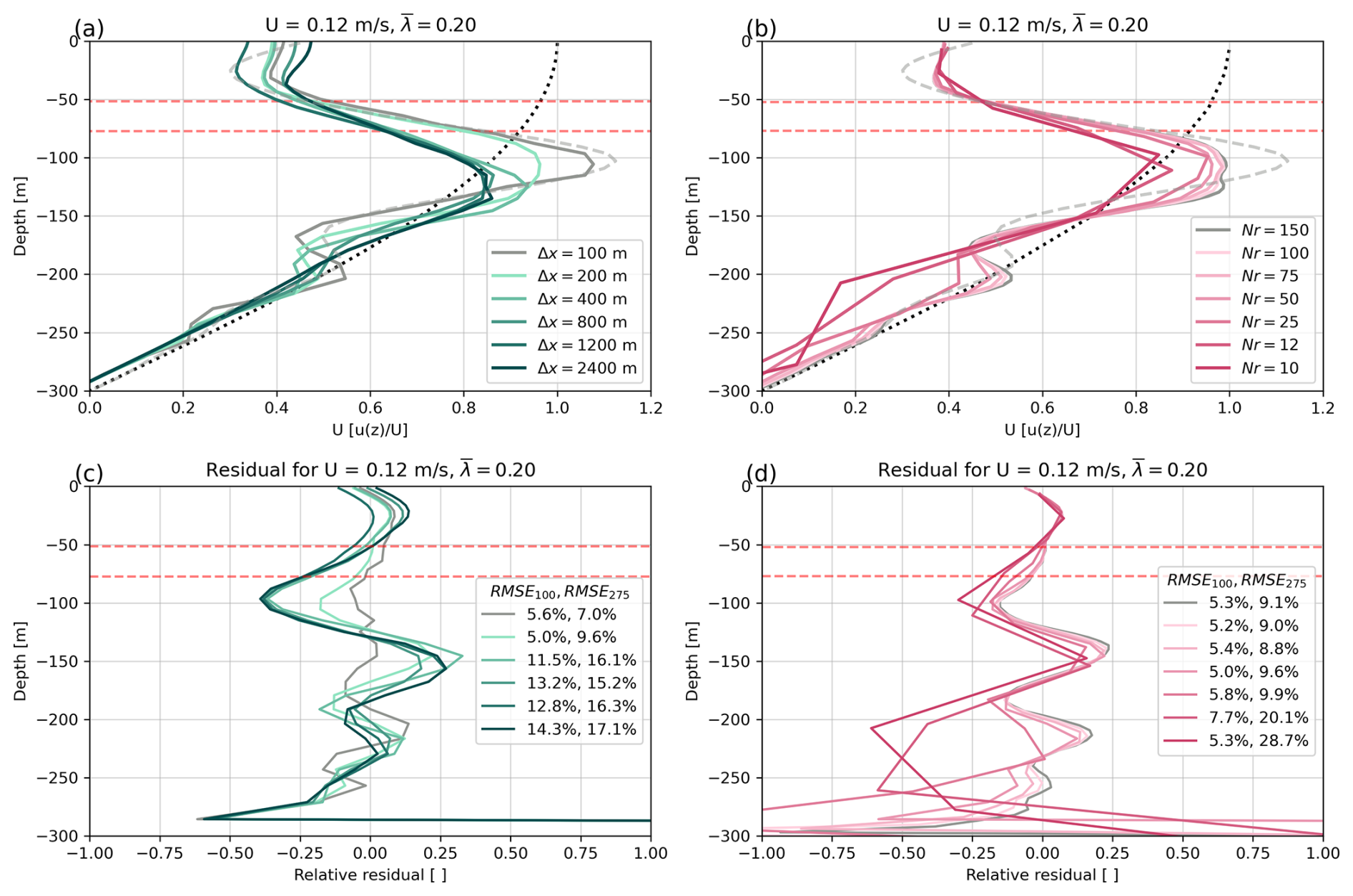
Figure 5 Ocean velocity averaged over the mélange pack for a range of Nr, Δx values for $U=\mathrm{0.12},\stackrel{\mathrm{‾}}{\mathit{\lambda }}=\mathrm{0.2}$. The dotted black line is the driving velocity, and the coarse gray line is the results from Hughes (2022) for the same U,λ. Dashed red lines are the median and 90th percentile of iceberg draft. Panels (c) and (d) show the relative residual ϵ (Eq. 8) for (a) and (b) respectively and list the RMSE₁₀₀ and RMSE₂₇₅ for each case in the legend. Panels (c) and (d) share the color scale of (a) and (b) respectively.

We find that the overall behavior of our parameterization is not significantly dependent on model resolution. We see the greatest reduction in RMSE₁₀₀ as the horizontal grid resolution approaches the length of the largest icebergs (200 m here) and when vertical resolution allows for more than 10 layers to resolve the full range of iceberg drafts (Nr=25 here). Model performance depends on the number of vertical layers available to capture the sinusoidal variation in velocity with depth. The wavelength of this sinusoidal variation falls beneath the resolution of the coarsest vertical grids we consider here ($Nr=\mathrm{10},\mathrm{12}$); thus RMSE₂₇₅ is particularly high (>20 % of driving velocity) for the coarsest Nr as the model is unable to resolve the deeper velocity maximum at ∼ 200 m depth (Fig. 5b). For horizontal grid scales, as the grid size approaches the size of the largest icebergs, our parameterization begins to have increasingly full cells, closely resembling the fully dry cells of the iceberg-resolving model. In this limit, our parameterization begins to individually resolve the largest icebergs within the pack, and thus our model more closely matches the iceberg-resolving model. This illustrates how our parameterization converges towards a model that fully resolves icebergs, and thus the residual decreases with increasingly fine horizontal resolution. However, once the horizontal grid size is more than double the largest icebergs (Δx=400 m here), further coarsening does not significantly reduce the performance of our parameterization, with a RMSE₁₀₀ of just 14 % of driving velocity for the Δx=2400 m case.

In summary, we find our parameterization of iceberg drag has satisfactory performance across a range of conditions and grid sizes. However, this benchmarking neglects the impact of freshwater production from melting and is not yet clearly compared to existing drag-free iceberg models.

4.2 Impact of blocking, drag, and melting

To investigate the impact of iceberg melting, we step outside the parameter space considered by Hughes (2022) and consider the impact of iceberg melting, drag, and blocking individually in the same idealized forced-flow domain. By isolating each of these effects, we showcase the impact of each mechanism, and this also allows us to compare our drag-enabled iceberg models against existing drag-free models (e.g., Davison et al., 2020). Specifically, we consider the $\stackrel{\mathrm{‾}}{\mathit{\lambda }}=\mathrm{0.2}$ and U=0.12 m s⁻¹ cases of FF_NoBlockDragMelt, FF_NoDragMelt, and FF_NoMelt (Table 2). We consider each of these three cases without melting, as well as the corresponding three melt-enabled cases, FF_NoBlockDrag, FF_NoDrag, and FF. We plot the mélange-averaged ocean velocities and net freshwater flux in Fig. 6. The FF_NoMelt case is the exact same as that in Sect. 4, and the FF_NoBlockDrag case is equivalent to that considered by Davison et al. (2020), Davison et al. (2022), Kajanto et al. (2023), Hager et al. (2024), and Slater et al. (2025).

In the no-melt cases, the competing effects of blocking and drag are well highlighted. The FF_NoBlockDragMelt case reproduces the driving current very well as expected, as there is no iceberg interaction with the ocean for this case. The FF_NoDragMelt case, however, accelerates the driving velocity in the upper 100 m by up to 150 %, which is a result of the flow being squeezed by the reduced effective volume of iceberg-filled cells, without any slowing effects of drag. In contrast, the FF_NoMelt case slows flow in the upper 100 m, as discussed in Sect. 4, when both blocking and drag are applied. The oscillatory form of velocity as a function of depth for the FF_NoDragMelt case follows a wavelength similar to that seen in Sect. 4 but has the opposite sign, with flows that are faster than the driving velocity above 100 m and slower than the driving velocity for 100–150 m (Fig. 6a).

When we consider the effect of melt on these three cases, the FF_NoBlockDrag case on average tracks the driving velocity but exhibits a vertical oscillatory behavior, with a wavelength that is also comparable, but with an opposite sign, to results in Sect. 4. The surface acceleration of the FF_NoBlockDrag case is driven by the injection of meltwater into the mélange. The FF_NoDrag case similarly sees an acceleration at the surface and a slowdown from 10–50 m depth compared to the FF_NoDragMelt case. Below 75 m, the 90th percentile for iceberg draft, the FF_NoBlockDrag and FF_NoDrag cases become very similar in ocean velocity. The FF and FF_NoMelt cases are very similar at all depths, as any impact of freshwater injection into the mélange is immediately overcome by drag.

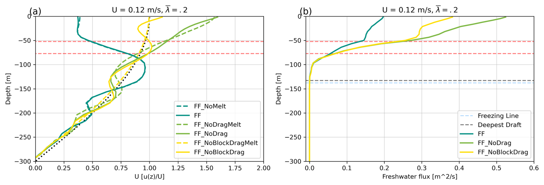
Figure 6 (a) Ocean velocity averaged over the mélange pack for a range of blocking, drag, and melt options for U=0.12, $\stackrel{\mathrm{‾}}{\mathit{\lambda }}=\mathrm{0.2}$. The dotted black line is the driving velocity. Dashed red lines are the median and 90th percentile of iceberg draft. (b) Freshwater production rates, averaged over the mélange pack, per unit depth for a range of block and drag options. No melt cases are omitted. Dashed red lines are the median and 90th percentile of iceberg draft, the dashed black line is the deepest draft, and the dashed blue line is the depth where the ambient temperature drops below freezing point.

Considering the impact of blocking and drag on melt rate in Fig. 6b, we find that the freshwater flux varies by up to 250 % between these cases. The greatest difference in freshwater flux is at the surface, where velocities are the most different as well. As suggested by the velocity-dependent form of our melt parameterization (Jenkins, 2011), the fastest case (FF_NoDrag) produced the highest freshwater flux of up to 0.5 m² s⁻¹ at the surface, while the FF case had the lowest freshwater flux of 0.2 m² s⁻¹ at the surface. The FF_NoDrag and FF_NoBlockDrag cases have very similar freshwater fluxes below 50 m, the median iceberg draft. In all cases, freshwater flux decreases as the total surface area of icebergs diminishes with increasing depth. Additionally, there is reduced thermal forcing with increasing depth as the ambient temperature approaches freezing point at $z=-\mathrm{137}$ m, as shown by the dashed blue line in Fig. 6b.

This section illustrates the impact of parameterized iceberg drag when modeling iceberg melt in an idealized scenario. Importantly, we find that for the FF case, results are very similar to those of the benchmarked FF_NoMelt case. This gives us confidence that our drag parameterization can successfully be applied in conditions including iceberg melt, which we explore in the next section.

5 Mélange melt domain results

We next consider the impact of iceberg drag on the coupled thermomechanical system of iceberg melting in a more realistic ocean domain. We again use results from an iceberg-resolving model as a benchmark for comparison (Hughes, 2024) and run our coarser-scale model in a comparable geometry to evaluate its performance. For these cases with melt, we run our coarse model with melting enabled in two settings: with blocking and drag enabled (MM) and with blocking and drag disabled (MM_NoBlockDrag, setting barrierMask = false). This MM_NoBlockDrag configuration is equivalent to the FF_NoBlockDrag case above and previous studies using the iceberg package (e.g., Davison et al., 2020). Details of this configuration are listed in Sect. 3.1 and visualized in Fig. 7. Notably, this system is driven only by ambient iceberg melt and is not forced by any subglacial discharge or other prescribed ocean velocity.

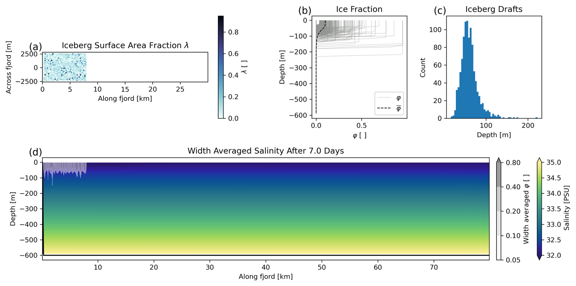
Figure 7 The configuration of our model domain for the mélange melt with blocking case. (a) Distribution of λ across the mélange pack. (b) Depth variance of φ. Light gray shows φ(z) of every cell containing icebergs, and the dashed black line shows the average φ over the entire mélange area, $\stackrel{\mathrm{‾}}{\mathit{\phi }}\left(z\right)$. (c) Histogram of iceberg drafts. (d) Width-averaged salinity of our model domain at the end of the simulation. Cells are shaded with the width-averaged value of φ to illustrate the location of the mélange pack.

Figure 8 Comparison of mélange melt model results for $z=-\mathrm{10}$ m. Temperature (left) and along-fjord velocity (right) are plotted for three cases. Icebergs are plotted in gray in the iceberg-resolving model of Hughes (2024) (a, b).

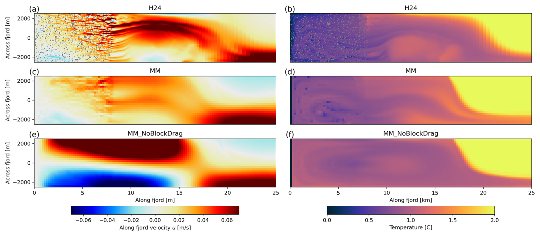
We compare our results directly against the results published by Hughes (2024), considering a horizontal slice at $z=-\mathrm{10}$ m depth and statistical results of ocean velocity and freshwater flux from melt. Figure 8 shows temperature and along-fjord velocities for all three cases (H24, MM, and MM_NoBlockDrag) for the horizontal slice $z=-\mathrm{10}$ m depth. Our full iceberg parameterization that includes drag and blocking (MM) replicates the main features of the H24 case, whereas the parameterization without blocking and drag (MM_NoBlockDrag) shows significantly different signals in the circulation patterns and magnitude of flow. This is particularly evident in the southern region of our domain ($y<-\mathrm{1000}$ m), where the MM_NoBlockDrag case shows a large region of return flow (u<0) towards the glacier front that is not present in the H24 or MM cases. Within the mélange pack, velocities in the H24 case are more detailed than in either coarse model, with regions of fast channelized flow or “hot spots”, as described in Hughes (2022, 2024) (Fig. 8a). This effect is not entirely absent in our MM coarse model (Fig. 8c), where some channelization is apparent as our grid scale of 200 m begins to resolve some of the largest icebergs. This effect of smoothing modeled velocity is largely an artifact of the limitations of a coarser-resolution model, and the overall form of the average velocity field is better captured by the coarse model MM than the coarse model MM_NoBlockDrag.

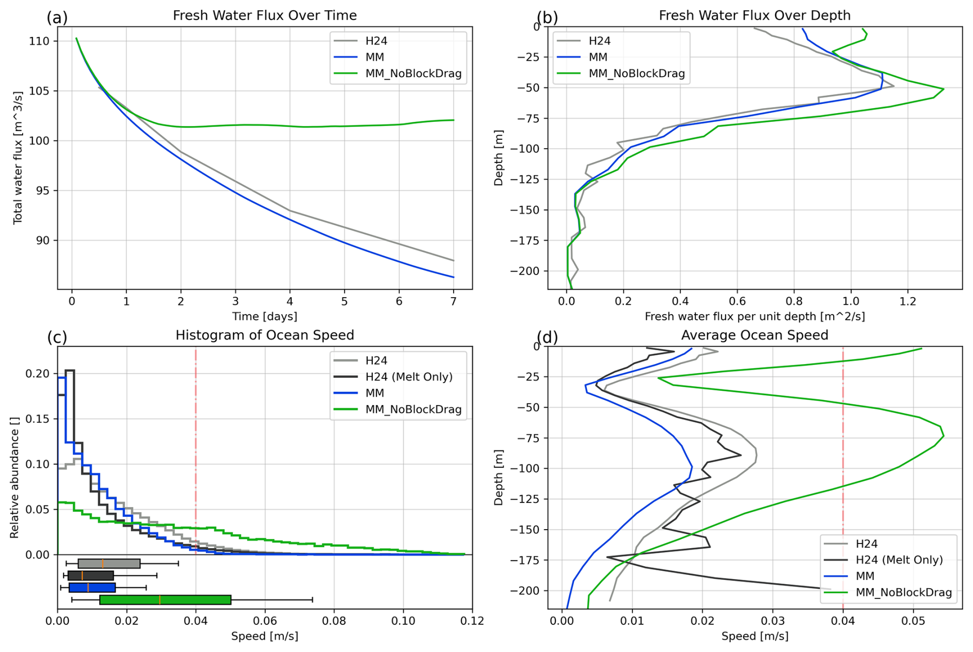
Figure 9 Impact of iceberg drag on meltwater production. (a) Total meltwater production over time; (b) meltwater production over depth; and (c) histogram of ocean speed within the mélange pack, with whisker plots showing the 10th, 25th, 50th, 75th, and 90th percentiles. (d) Average ocean speed across the mélange pack as a function of depth. The dash-dot red line in (c) and (d) is the minimum melting velocity used in our melt parameterization. Panels (b)–(d) show values averaged over the final 2 h of the simulation.

We track the overall freshwater flux across the entire mélange as a function of time and depth for the H24, MM, and MM_NoBlockDrag cases (Fig. 9a, b). The MM case reproduces the freshwater flux of Hughes (2024) with an error of 2.1 % compared to 16 % error for the MM_NoBlockDrag case. Freshwater flux for the MM case decreases steadily throughout the model run, consistent with the H24 case (Fig. 9a). This is in contrast to the MM_NoBlockDrag case, which has deceasing flux for the first day but then levels off to a roughly constant freshwater flux, resulting in a 16 % higher total freshwater flux on day 7 compared to H24. The distribution of freshwater flux in Hughes (2024) as a function of depth is also well reproduced in the MM case, which both show a depth of maximum freshwater flux at 50 m and a near-linear reduction in freshwater flux in the upper 50 m (Fig. 9b). The MM_NoBlockDrag case shows higher freshwater flux across the entire fjord depth, as well as a second local maximum of freshwater flux near the surface.

We report the ocean speed ($(u^{\mathrm{2}}+v^{\mathrm{2}}+w^{\mathrm{2}}{)}^{\mathrm{1}/\mathrm{2}}$) across the ice mélange for the final 2 h of the simulation in a histogram of ocean speed for all ocean cells within the ice mélange (Fig. 9c) and as box and whisker plots showing the 10th, 25th, 50th, 75th, and 90th percentiles. We consider the depth variation in average ocean speed for the final 2 h of the simulation within the ice mélange in Fig. 9d as ocean speed is a primary control on melt rates (Jenkins, 2011). The dash-dot red line in Fig. 9c and d highlights the minimum melting velocity used in our melt parameterization, so variations in ocean speed above this value will drive changes in the parameterized melt rate. In Fig. 9c and d, we report the H24 values for the entire mélange (gray) and for only the cells that are in direct contact with ice and thus impact melt (dark gray). For H24 this is approximately 5 % of the cells within the ice mélange. In our coarse model, all cells in the mélange pack are in contact with ice. The MM_NoBlockDrag case shows significantly faster ocean speeds compared to H24 melt-only speeds. The MM ocean speeds are very similar to the H24 melt-only speeds but are slightly slower by 0.005 m s⁻¹ for the 90th percentile value. In Fig. 9d, we show that this slower ocean speed for the MM case compared to the H24 melt-only speed is concentrated below 50 m depth. Though all cases show a minimum in average ocean speed at around 30 m, the MM_NoBlockDrag case has consistently higher ocean speeds compared to H24 above 150 m depth.

Thus, we have shown that our iceberg parameterization with full drag and blocking effects (MM) captures much of the behavior of the iceberg-solving model of H24 while at a significantly coarser resolution. Further, the MM case significantly outperforms the case with melt but no blocking and no drag (MM_NoBlockDrag).

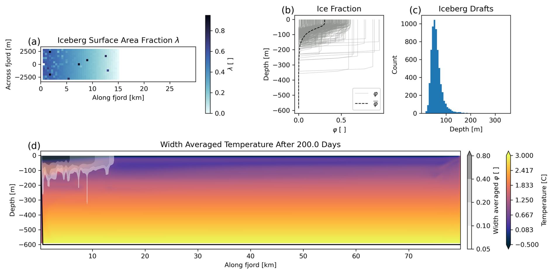
Figure 10 The configuration of our model domain for the full fjord run. (a) Distribution of λ across the mélange pack. (b) Depth variance of φ. Light gray shows φ(z) of every cell containing icebergs, and the dashed black line shows the average φ over the entire mélange area, $\stackrel{\mathrm{‾}}{\mathit{\phi }}\left(z\right)$. (c) Histogram of iceberg drafts. (d) Width-averaged temperature of our model domain at the end of the simulation. Cells are shaded with the width-averaged value of φ to illustrate the location of the mélange pack.

6 Fjord-scale domain results

As a final case, we demonstrate the computational scalability of our parameterization for a quasi-realistic mélange-filled fjord system (Fig. 10) driven by 500 m³ s⁻¹ of subglacial discharge (SGD). Details of this configuration are described in Sect. 3.1. To compare the net effect of icebergs and iceberg drag, we now consider three cases: FJ_NoIcebergs, where there is no melting, no blocking, and no drag from icebergs (i.e., no impact from icebergs and the iceberg2 package is disabled); FJ_NoBlockDrag, where we include iceberg melt with no blocking and no drag; and FJ, where iceberg melt, blocking, and drag are all included. It is important to note that almost all regional ocean model simulations in which Greenlandic fjords are resolved (Gladish et al., 2015; Carroll et al., 2017; Wood et al., 2024) are equivalent to the FJ_NoIcebergs case. Relatedly, all prior studies using the iceberg package (Davison et al., 2020, 2022; Kajanto et al., 2023; Hager et al., 2024; Slater et al., 2025) are equivalent to the FJ_NoBlockDrag case. We focus on three metrics: total freshwater flux, near-glacier temperature, and mid-fjord average velocity (Fig. 11). Freshwater flux is the sum of subglacial discharge, glacier frontal melting, and iceberg/mélange melting; near-glacier temperature is the average temperature over the 800 m (two grid cells) of the ocean closest to the glacier terminus (similar to Davison et al., 2022; Hager et al., 2024); and the mid-fjord conditions are the along-fjord velocities spatially averaged over the region 20 km to 40 km from the glacier. Near-glacier and mid-fjord conditions are temporal averages of the final 18 d of our 200 d simulation. To highlight the north–south asymmetry of flow in the mid-fjord region, we divide mid-fjord conditions into north and south halves of the fjord in Fig. 11 and plot slices of the along-fjord velocity, u, in Fig. 12. We plot the map view of u at $z=-\mathrm{100}$ m of the entire fjord (Fig. 12a, c, e) and the across-fjord profile of the average u for the mid-fjord region (Fig. 12b, d, f) for the FJ_NoIcebergs, FJ_NoBlockDrag, and FJ cases respectively.

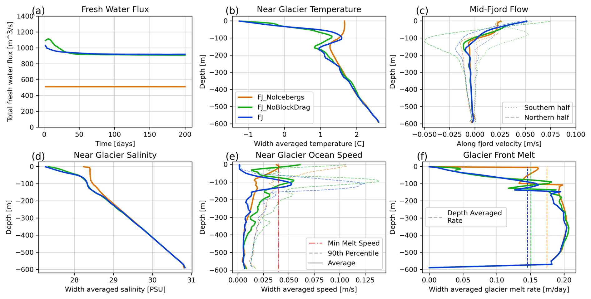
Figure 11 Impact of icebergs and drag on fjord level values. (a) Total freshwater flux, including subglacial discharge and iceberg/mélange melt for the full 200 d. (b) Average temperature within 800 m of the glacier terminus. (c) Average along-fjord ocean velocity in the mid-fjord region. Dashed lines show the northern half of the fjord, dotted lines show the southern half of the fjord, and solid lines are the average across the entire width. (d) Average salinity within 800 m of the glacier terminus averaged over the final 18 d. (e) Average ocean speed within 800 m of the glacier terminus. (f) Glacier front melt rates, averaged across the fjord, with depth-averaged values also plotted as a dashed line. Panels (b)–(f) are all averaged over the final 18 d. All frames share the color legend of panel (b).

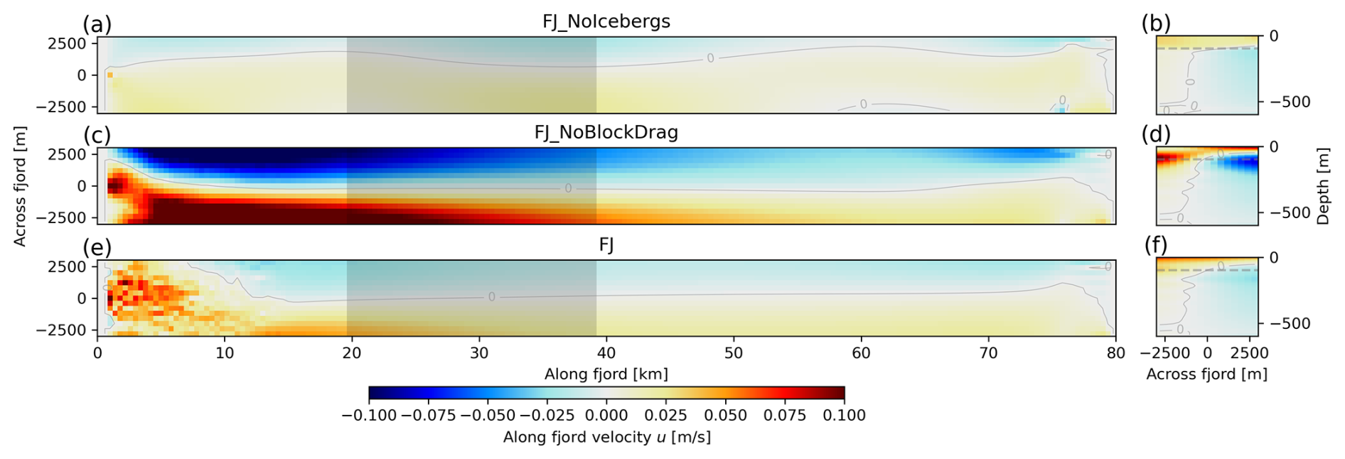
Figure 12 Comparison of fjord-scale domain results in map view for $z=-\mathrm{100}$ m (a, c, e) and cross-sectional view of the mid-fjord region (b, d, f) for along-fjord velocity u. Panels (a) and (b) show along-fjord velocity for the FJ_NoIcebergs case. Panels (c) and (d) show along-fjord velocity for the FJ_NoBlockDrag case. Panels (e) and (f) show along-fjord velocity for the FJ case. The gray-shaded region in (a), (c), and (e) is the mid-fjord region that is shown in panels (b), (d), and (f) respectively. The dashed gray line in (b), (d), and (f) is the −100 m depth that is shown in the map view in panels (a), (c), and (e) respectively. In all panels, the u=0 contour is plotted as a thin gray line. All panels are temporally averaged over the final 18 d of the simulation.

Our results show that icebergs significantly modify fjord conditions by increasing freshwater flux into the ocean, cooling glacier-adjacent conditions, and modifying the overturning flow, in agreement with other studies of iceberg impacts on fjord dynamics (Enderlin et al., 2016; Davison et al., 2020, 2022; Kajanto et al., 2023; Hager et al., 2024). However, we note that the inclusion of iceberg drag impacts the magnitude of these effects. Namely, the FJ case has 0.25 °C warmer near-glacier temperatures at 50–150 m depth compared to the FJ_NoBlockDrag case (Fig. 11b). This is the terminal height of the subglacial plume (velocity maximum in Fig. 11e); thus we argue that this warmth arises from the plume becoming trapped within the mélange. The FJ case has a slower and deeper return flow compared to the FJ_NoBlockDrag case at 100–200 m depth (Fig. 11c). The impact on mid-fjord flow is the most apparent in comparing the average along-flow velocity of the northern and southern halves of the fjord, where we see a much smaller north–south velocity contrast and overall slower flow in the FJ case compared to the FJ_NoBlockDrag case (Fig. 12). The finding of slower ocean velocities in the FJ case extends to the glacier front: Fig. 11e shows near-glacier ocean speeds, with the FJ case having overall slower speeds compared to the FJ_NoBlockDrag case. Figure 11d shows the impact of icebergs on freshening near-glacier water, but this trend is not significantly impacted by iceberg drag. The competing effects of warmer water and slower flow on glacier front melt rates largely cancel out in our study, with very slightly lower vertically averaged glacial melt rates for the FJ case compared to the FJ_NoBlockDrag case, though both cases exhibit lower glacier melt rates than the FJ_NoIcebergs case (Fig. 11f). For terminus melt parameterizations that are sensitive to ocean velocities below 0.04 m s⁻¹, we would expect a much larger difference in glacial melt rates between the FJ and FJ_NoBlockDrag cases. The full effect of mélange, ice drag, and subglacial discharge plumes on terminus melt rates is the subject of ongoing work and is beyond the scope of this study.

Relatedly, the overall freshwater flux from iceberg melt is similar after more than 20 d in the FJ_NoBlockDrag and FJ cases (Fig. 11a). The initial disparity between these two (before day 20) matches the disparity observed in Sect. 5, which we explained by much higher ocean velocities in the no-drag case. After day 20, the FJ_NoBlockDrag case still exhibits faster flow within the mélange, but this is balanced by colder and fresher conditions within the mélange (Fig. 11b), an effect that takes a few days to spin up and was thus missed in our 7 d scenario. This match in freshwater flux only exists for the total net flux as the FJ_NoBlockDrag case produces a large north–south asymmetry in freshwater flux across the mélange not present in the FJ case, as discussed in Appendix C.

Each fjord model was run on 20 cores across 2 nodes with a total wall time of 03:12:04 for the FJ_NoIcebergs case, 04:28:52 for the FJ_NoBlockDrag case (28 % slower), and 04:28:26 for the FJ case (31 % slower than FJ_NoIcebergs, comparable to FJ_NoBlockDrag). The FJ case should be more computationally expensive compared to the FJ_NoBlockDrag case, but this effect is less than the magnitude of random variability in model runtimes. Given the ∼ 90 % speed-up we built into iceberg2 and the minimal computational cost of including drag, iceberg2 enables more performant fjord-scale simulations. To simulate our fjord with iceberg melt and parameterized iceberg drag (FF case), this equates to 13.3 core hours per month of fjord simulation time, enabling scalable simulations at timescales of multiple months to multiple decades. We did not attempt to run an iceberg-resolving model like Hughes (2024) for this fjord-scale geometry, but scaling our FJ_NoIcebergs case runtime linearly with the number of grid cells and time steps for a $\mathrm{\Delta }x=\mathrm{\Delta }y=\mathrm{10}$ m, Nr=64 run would result in a computational cost of over 17 core years per month of fjord simulation time, roughly 10 000× the computational expense. To summarize, we find that icebergs drive cooler, fresher, and faster fjord conditions compared to an iceberg-free fjord, and iceberg drag moderates some of the effects. Namely, iceberg drag slows and slightly warms fjord conditions compared to models that lack iceberg drag.

7 Discussion

Icebergs and ice mélange have previously been modeled at a range of scales and realism, with widely varied computational demands. In this work, we develop a scalable parameterization to include the processes of melt as well as blocking and drag. Our model builds upon previous versions of iceberg (e.g., Davison et al., 2020) and complements existing approaches of modeling icebergs and ice mélange, including iceberg-resolving models (Hughes, 2022, 2024; Jain et al., 2025) and simplified ice-shelf-like approaches (Wood et al., 2025). Iceberg-resolving models are specifically designed for capturing the nature of ocean flow around icebergs, but due to computational requirements, they are not realistically scalable to fjord-scale, long-duration simulations. Thus, we benchmark our model's performance against that of iceberg-resolving models and demonstrate that iceberg drag impacts important near-terminus and fjord-wide processes. Previous versions of iceberg have captured the 3D geometry of icebergs when resolving melt processes but have omitted drag processes. We extend this package to include a parameterization of iceberg drag and demonstrate the impact drag has on model results for an idealized fjord. Ice-shelf-like approaches to modeling ice mélange utilize the shelfice MITgcm package, which only resolves drag and melting at the bottom layer of the mélange and completely blocks ocean flow within the mélange. This trade-off in realism comes with significant computational efficiencies compared to iceberg-resolving models and previous versions of iceberg. Our work improves the computational efficiency of iceberg2, now offering computational performance of the same order of magnitude as ice-shelf-like approaches. In limited testing (not shown), our model is ∼ 150 % slower than ice-shelf-like mélange models, while offering significantly improved model realism.

Iceberg and terminus melt rates are expected to be strongly dependent on the ocean velocity adjacent to the ice. These velocities are set by a combination of far-field (tens to hundreds of meters) ocean dynamics and also near-ice ambient melt plume speeds (Slater et al., 2015; FitzMaurice et al., 2017; Zhao et al., 2024). The effect of sub-grid-scale ambient plumes is commonly included in models by imposing a minimum velocity to be used in the three-equation melt parameterization (Slater et al., 2015; Zhao et al., 2024). For the simulations that we have run here, the velocities within the mélange are relatively weak (mean ∼ 0.02 m s⁻¹) and often below this minimum velocity threshold. Thus, the melt rates we report are sensitive to the choice of this minimum velocity threshold, similar to those of Hughes (2024). However, the statistics of the ocean conditions (velocity and temperature) in the ice-adjacent cells are very similar between the iceberg-resolved simulations (Δx=10 m) and our iceberg-parameterized runs (Δx=200 m). The consistency of modeled iceberg-adjacent ocean conditions across modeling scales suggests that both ∼ 10 and ≥ 10² m models (e.g., Hughes, 2024; Jain et al., 2025, this study) produce reasonable far-field ocean conditions but that they are still strongly dependent on their ambient plume parameterization for calculating melt rates.

A clear compromise of our coarser model, compared to iceberg-resolving models, is that it does not capture fine details of ocean flow. This is particularly evident in the lack of so-called “hot spots”, regions with substantially faster flow (u>0.05 m s⁻¹) where water squeezes between icebergs (Fig. 8a), as discussed in Hughes (2024). However, Fig. 9c highlights how these “hot spots” of faster flow are disproportionally not in contact with icebergs, and the statistics of the speed of ocean cells in contact with icebergs, which are actually used to calculate melt rates (H24, melt only), are well reproduced by our coarse model MM (Fig. 9c, d). Overall, the MM case slightly under-predicts ocean speeds and melt rates (2.1 % meltwater flux error), but it seems that the impact of these “hot spots” on melt rate may be moderated by processes providing physical insulation of icebergs from these fastest flows. An important finding here is that, although our melt parameterization enforces a minimum melt speed of 0.04 m s⁻¹, our MM case effectively matches ocean speeds in cells in contact with icebergs in the H24 case, even below this speed (Fig. 9c). Thus, we expect our MM case to retain its skill at matching melt rates to the iceberg-resolving H24 case, even subject to changes in this minimum melting speed, like those discussed in Zhao et al. (2024).

When we apply this model to a multi-month fjord run, we identify the net effects of iceberg melt, blocking, and drag on overall fjord conditions. Specifically, our results agree with previous studies that icebergs significantly increase overall freshwater flux (Enderlin et al., 2016), cool the near-glacier conditions (Davison et al., 2022; Hager et al., 2024), and increase the net exchange flux (Davison et al., 2020; Kajanto et al., 2023). Our results here show that all of these findings are modified by including iceberg blocking and drag (FJ), generally reducing the magnitude of each effect compared to numerical models without iceberg blocking and drag (FJ_NoBlockDrag).

Without blocking and drag, we find that a strong cross-fjord asymmetry develops in near-glacier conditions, with up to a 0.5 °C temperature difference and a 60 % difference in freshwater flux across the fjord (Fig. C1). However, cross-fjord gradients are substantially reduced when we include the most realistic effects of blocking and drag (FJ case), where there is almost no cross-fjord variation in temperature or freshwater flux. These errors (faster flow and lower temperatures in FJ_NoBlockDrag compared to FJ) could counteract each other in the calculation of melt, perhaps explaining why studies using the previous version of iceberg (Davison et al., 2022; Hager et al., 2024) yielded reasonable overall freshwater flux values, despite omitting iceberg drag. Although these errors are roughly offset for the FJ_NoBlockDrag case here, it is not clear whether this is a reliable trend, and we show that drag-free simulations do not reliably reproduce the spatial distribution of mélange melt. Further, the distribution of mélange melt directly impacts mélange thickness, which could have significant effects on the mechanical strength of the mélange and thus impact glacier calving rates (Amundson et al., 2010; Robel, 2017; Amundson et al., 2025). Strong asymmetries in mélange melting would likely mechanically weaken the mélange more than uniform melting, particularly if melt is concentrated in bands near walls, which can contribute buttressing shear stresses (Robel, 2017; Amundson et al., 2025). Thus, we argue that iceberg drag is an important factor to consider for mélange melt dynamics, even if the spatially averaged melt rate is not significantly different between the specific cases, FJ and FJ_NoBlockDrag, considered here.

8 Conclusions

In this study, we describe a parameterization of the effect of sub-grid-scale iceberg blocking and drag in the context of a rigid ice mélange. To demonstrate the accuracy and computational performance of this parameterization, we implement it as an improvement to the iceberg2 package in MITgcm and benchmark it against an iceberg-resolving model in idealized simulations. Our parameterization offers reasonable accuracy (RMSE₁₀₀ of 6 % of driving velocity) across a wide range of parameter values and grid scales (Figs. 4, 5) at a drastically lower ($\mathrm{1}/\mathrm{10}\mathrm{000}\times$) computational expense. In our benchmarking case that includes iceberg melt, our parameterization of drag reproduces fjord-scale features with improved fidelity to the iceberg-resolving model compared to a simulation without drag. Specifically, our parameterization of iceberg drag better matches the freshwater production rate and overall velocity structure of the ocean compared to a simulation without drag. When we apply our model to a multi-month fjord-scale simulation, we find that icebergs cool, freshen, and increase overall circulation within the fjord, in line with previous work (e.g., Davison et al., 2020; Kajanto et al., 2023; Hager et al., 2024), though all of these effects are modified by the inclusion of iceberg drag. Namely, iceberg drag suppresses ocean currents and warms near-glacier water slightly compared to the no-drag case when a subglacial plume is present. Overall, the net effects of icebergs and drag on fjord conditions are most apparent within the ice mélange, cooling near-surface waters and injecting freshwater, but effects are also seen in altered ocean currents more than tens of kilometers down the fjord.

This work takes an important step toward more realistically capturing the complexities of coupled iceberg–ocean interactions within fjords and enables more readily scalable computational methods for including iceberg drag effects at fjord and larger scales. We demonstrate the scalability of our method to a multi-month fjord-scale model run and the importance of including the effect of both iceberg melt and iceberg drag on overall fjord dynamics. This innovation enables future efforts to simulate the co-evolution of icebergs and ocean circulation near ice sheets on multi-decadal and longer timescales.

Appendix A: Computational details and improvements

We include the effect of physical blocking by leveraging partially filled cells with the MITgcm grid (Adcroft et al., 1997). We set the three partially filled cell factors – hFacC, hFacS, and hFacW – for every cell and layer based on φ. Due to an implementation error in the previous version of iceberg, the commonly enabled non-linear free surface option in MITgcm unintentionally removes the hFacC, hFacS, and hFacW values set by previous versions of iceberg after the initial time step, which disables the blocking effect of icebergs after the initial time step (Davison et al., 2020, 2022; Kajanto et al., 2023; Hager et al., 2024; Slater et al., 2025). We discovered and validated this effect by inspecting the output hFacC, hFacS, and hFacW files at multiple time steps of model runs using the original iceberg. Thus, all previous studies using iceberg have inadvertently disabled the blocking effect after the first time step. In this updated iceberg2, we correct this implementation error, making the package compatible with the non-linear free surface option, though the non-linear free surface solver is not utilized here or in previous studies.

To enable testing of the updated iceberg2 with Hughes (2022) in Sect. 4, we run the model with iceberg melt disabled. This is accomplished by setting the iceberg2 flag meltMask = false for all cells containing icebergs. In a similar fashion, for the sweep of runs considered in Sect. 4.2, blocking and drag are disabled together by setting the iceberg2 flag barrierMask = false for all cells containing icebergs. This disables all blocking and drag effects from icebergs. Finally, drag alone is disabled by setting the iceberg flag barrierMask = true for all cells containing icebergs and setting the iceberg2 variable C_bd = 0, which causes icebergs to have 0 drag but still includes the blocking effect.

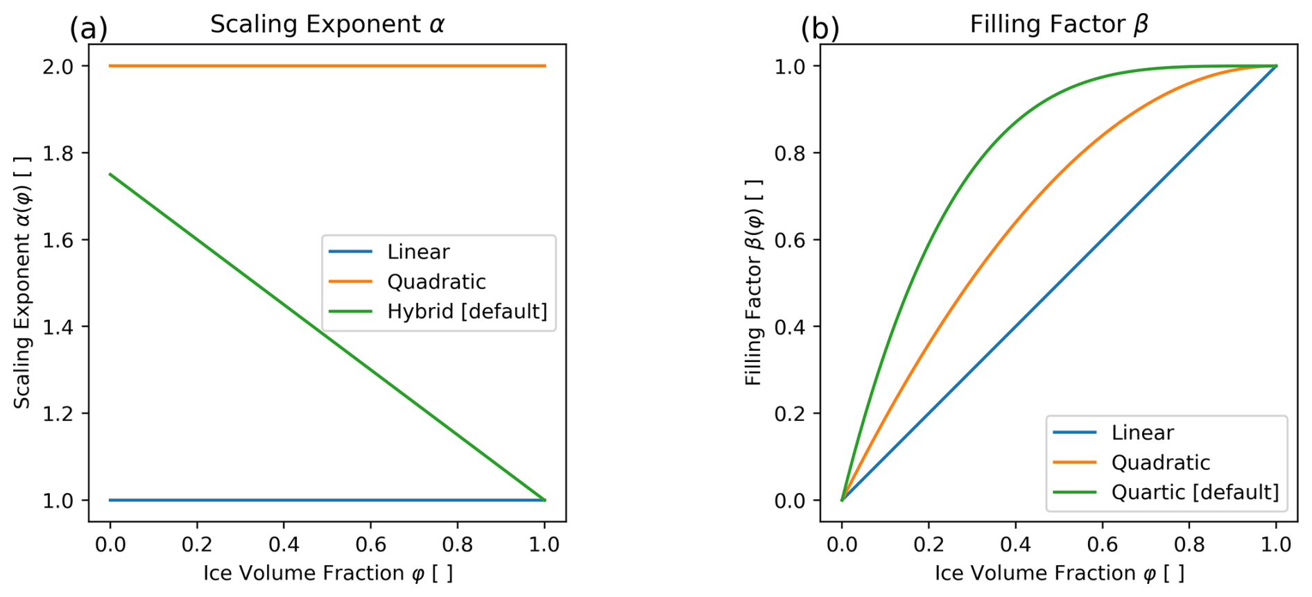
Figure A1 Visualization of the parameters α,β and their variation with ice volume fraction φ.

We plot the variation in the available α,β options within the new iceberg2 package over the range of ice volume fraction (φ) values in Fig. A1. Default values for both α and β are indicated in the legend.

With respect to runtime improvements in this update, previously within iceberg2, the geometry of each individual iceberg was stored as a text file and loaded for every time step of the MITgcm. For multi-month simulations, this can result in upwards of 10⁶ file load events. In this new iteration of iceberg2, at model initialization we load the geometries of all icebergs directly into memory using the READ_REC_3D_RL function. While this requires slightly more memory overhead to store icebergs in memory (∼ 10–100 MB), the reduction in file load events comes with an over 90 % improvement in computational performance. In a very small idealized fjord simulation (not shown), runtime was reduced from 2038 s with the text-file method to 170 s while loading all iceberg geometries directly to memory at initialization.

Appendix B: Selection of C_bd

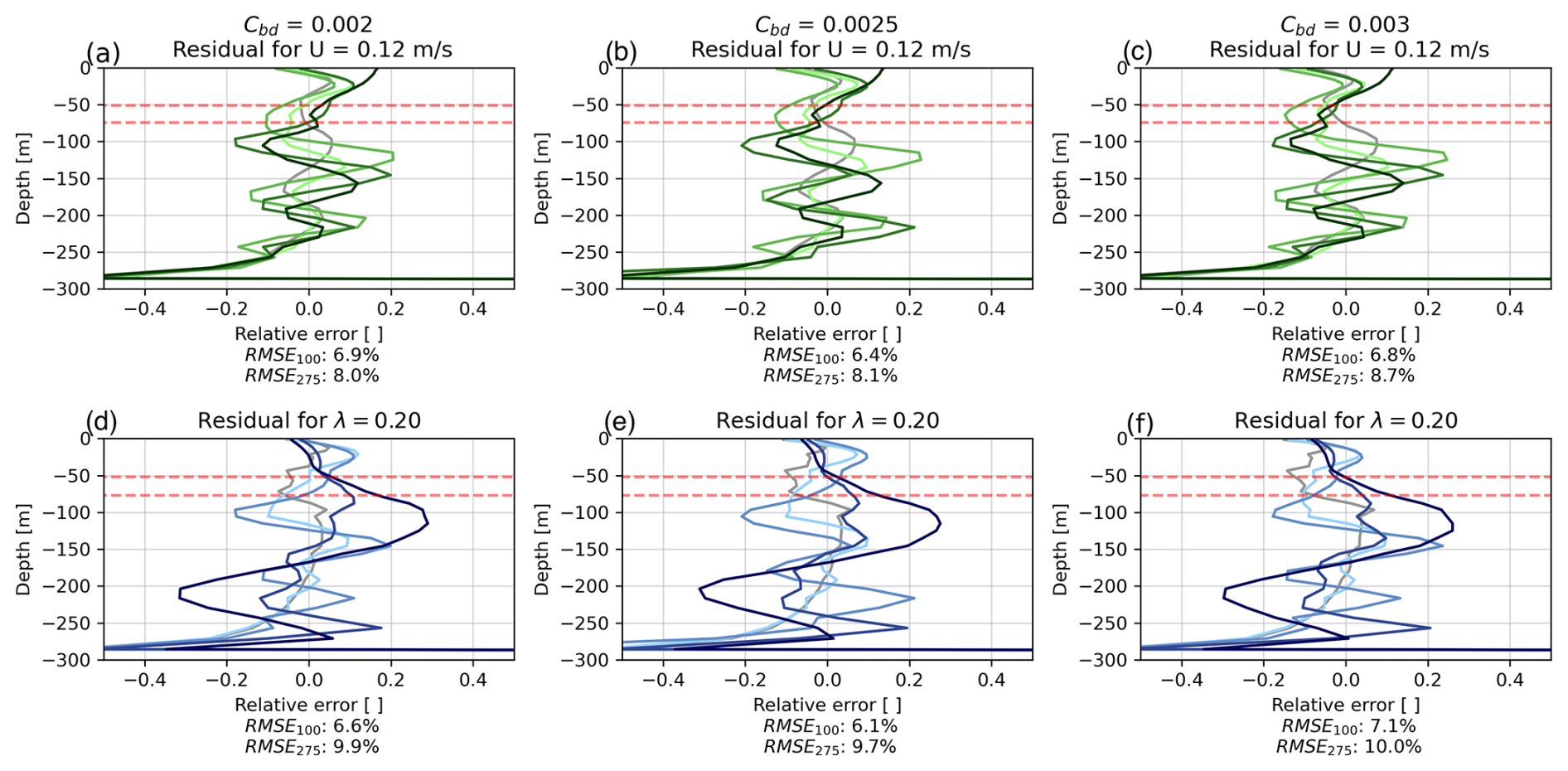
We investigate a range of C_bd values to gauge what order of magnitude would be appropriate for C_bd, before identifying 0.002–0.003 as the range for the most detailed consideration. We consider the full suite of model runs over λ,U, as discussed in Sect. 4, for each value of C_bd. For each C_bd, we compute the root mean squared error (RMSE) compared to results from Hughes (2022) for the upper 100 m, as this focuses on the match for ocean velocities within the bulk of the mélange, as well as the RMSE for the upper 275 m. We report the RMSE below each subplot for the upper 100 and 275 m. We find C_bd=0.0025 minimizes the RMSE₁₀₀ for the runs of λ=0.02–0.4 and U=0.12 m s⁻¹ (Fig. B1a–c) and the runs of λ=0.2 and U=0.02–0.40 m s⁻¹ (Fig. B1d–f). Figure B1 shares the same color legend as Fig. 4. The RMSE₁₀₀, i.e., the total root mean squared error in the upper 100 m of the ocean, across all λ,U cases considered for C_bd=0.0025 is 6.049 % of driving velocity.

Figure B1 Impact of varying C_bd on our fit to Hughes (2022). Primary effects are found in the upper 50 m, where slower velocities (more negative residuals) result from higher C_bd values. We select C_bd=0.0025 as this minimizes the overall RMSE₁₀₀.

Appendix C: Asymmetry of mélange conditions for fjord-scale run

To highlight the asymmetry of the behavior in the FJ_NoBlockDrag case, we plot freshwater flux from the mélange only (no SGD included here) and split the north and south halves of the fjord into separate domains, which we also plot in Fig. C1a. We similarly report glacier-adjacent conditions split by the north–south section of the domain in panel b. The FJ case shows very little north–south variation for both freshwater flux and glacier-adjacent temperature. In contrast, the FJ_NoBlockDrag case shows strong asymmetry, with 60 % more freshwater flux in the southern half than in the northern half. This melt asymmetry is partially explained by the 0.5 °C colder near-glacier conditions in the northern half of the fjord, which are caused by recirculating cold, fresh meltwater drawn back by a strong recirculating current like that shown in Fig. 8.

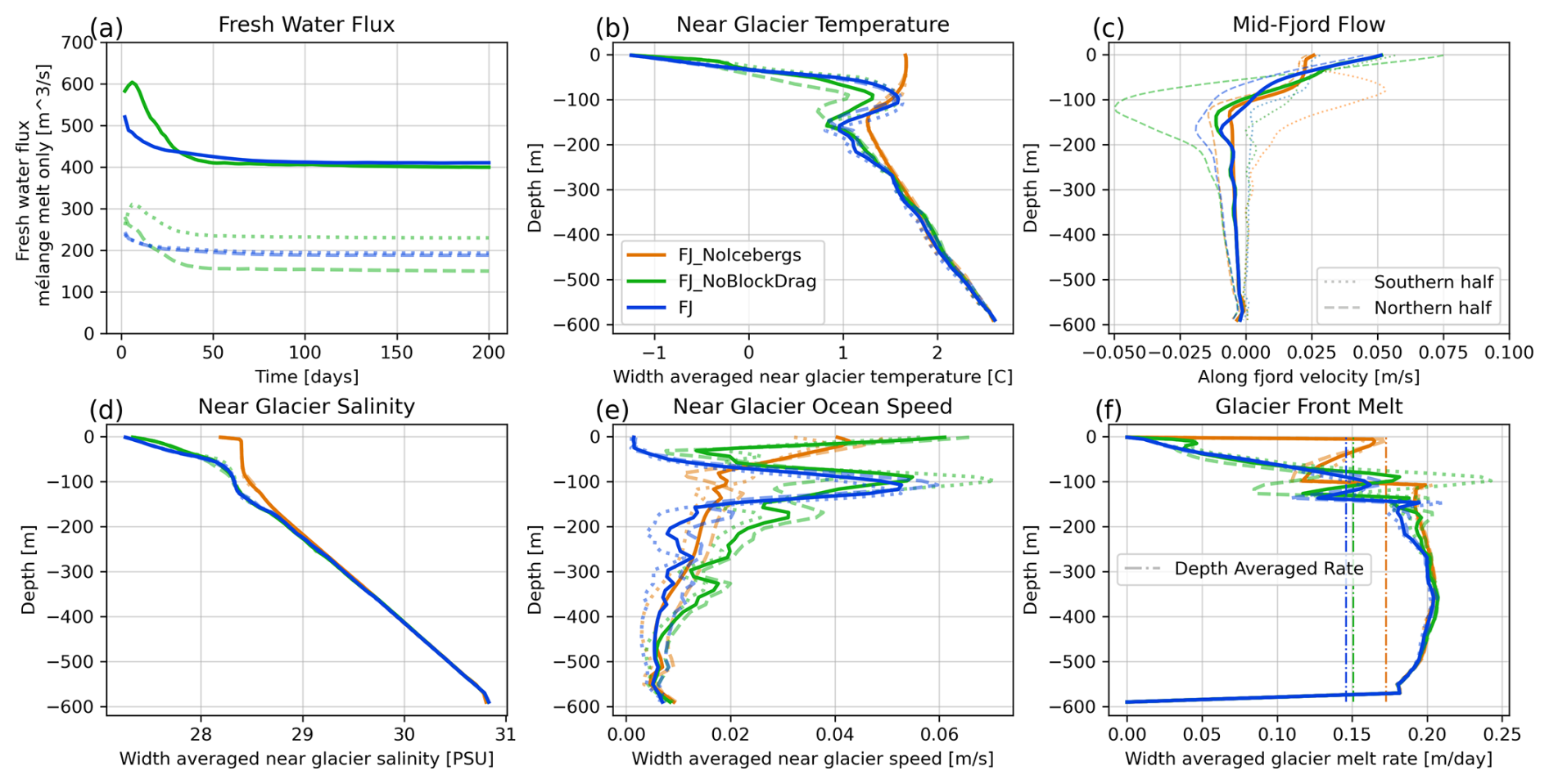
Figure C1 Impact of icebergs and drag on fjord level values. (a) Freshwater flux, including only mélange melt for the full 200 d. (b) Average temperature within 800 m of the glacier terminus. (c) Average along-fjord ocean velocity in the mid-fjord region averaged over the final 18 d. Dashed lines show the northern half of the fjord, dotted lines show the southern half of the fjord, and solid lines are the average across the entire width. (d) Average salinity within 800 m of the glacier terminus. (e) Average ocean speed within 800 m of the glacier terminus. (f) Average glacier front melting rate. All frames share the color legend of panel (b).