Combining observational data and numerical models to obtain a seamless high-temporal-resolution seasonal cycle of snow and ice mass balance at the MOSAiC Central Observatory

Multidisciplinary drifting Observatory for the Study of Arctic Climate (MOSAiC) observations span an entire annual cycle of Arctic snow and sea ice cover. However, the measurements of atmospheric and ocean forcing, as well as distributed measurements of snow and ice properties, were occasionally interrupted for logistical reasons. The most prolonged interruption happened during the onset of the summer melt season. Here we introduce and apply a novel data–model fusion system that can assimilate relevant observational data in a collection of modeling tools (SnowModel-LG and HIGHTSI) to provide continuous high-temporal-resolution (3-hourly) time series of snow and sea ice parameters over the entire annual cycle. We used this system to analyze differences between the three main ice types found in the MOSAiC Central Observatory: relatively deformed second-year ice, second-year ice with extensive smooth refrozen melt pond surfaces, and first-year ice. Since SnowModel-LG and HIGHTSI were used in a 1-D configuration, we used a sea ice dynamics term D to parameterize the redistribution of snow to newly created ridges and leads. D correlated highly with the sea ice deformation (R² = 59 %, N=33) in the vicinity of the observatory, and deformation appears to explain as much as 15 % of all winter snow water equivalent. In addition, we show, in separate simulations for level ice, that snow bedforms with thin snow in the bedform troughs largely control the ice growth. Here, the mean snow depth minus 1 standard deviation was required to simulate realistic sea ice thickness using HIGHTSI; we surmise that this accounts for the control of relatively thin snow on local ice growth. Despite different initial sea ice thickness and freeze-up dates, the sea ice thickness of level ice across all ice types became similar by early winter. Our simulations suggest that the mean (spatially distributed) MOSAiC snowmelt onset began in late May but was interrupted by a snowfall event and was delayed by 3 weeks until mid- June. The level ice started to melt in the last week of June. Depending on the sea ice topography, the ice was snow-free by late June and early July.

1 Introduction

Sea ice is an important regulator of the Arctic Ocean energy budget. Sea ice limits the transfer of energy (McPhee, 2012) and light (Arrigo et al., 2012) from the atmosphere to the ocean and constrains the transfer of heat from the ocean to the atmosphere (Maykut and Untersteiner, 1971). A strongly controlling component of this flux-dampening effect of sea ice is associated with the presence, quantity, and physical properties of snow that may cover it. Snow on sea ice is the main regulator of level sea ice thickness (Sturm et al., 2002b; Perovich et al., 2011; Itkin et al., 2023). Snow has an order of magnitude lower thermal conductivity than sea ice and, in winter, inhibits ice growth by insulating it from the relatively cold atmosphere (Maykut and Untersteiner, 1971; Sturm et al., 2002b). In summer, snow slows down sea ice melting by increasing the albedo (Perovich et al., 2011). These roles of snow governing sea ice evolution have become more evident with the general ice cover thinning taking place in association with recent climate change (Meredith et al., 2019). Now, both first-year ice (FYI) and second-year ice (SYI) can reach similar thicknesses at the end of the winter ice growth season (Itkin et al., 2023) and can reach similar melt pond distributions in summer (Webster et al., 2022).

Since the density and thermal properties of sea ice and snow are so different, both need to be accounted for in order to understand the state of the coupled snow–sea ice system. This remains one of the major challenges of satellite remote sensing of snow and sea ice in polar regions and, consequently, impacts the validation of climate models that rely on these data (Gerland et al., 2019). The drift of the Multidisciplinary drifting Observatory for the Study of Arctic Climate (MOSAiC) in 2019–2020 (Fig. 1) was the largest research expedition to the Arctic Ocean to date. It was implemented to help fulfill this need and others and had a key goal of collecting data relevant for climate process studies across the entire snow and sea ice annual cycle and to do so with a special focus on the less-studied winter period (Nicolaus et al., 2022).

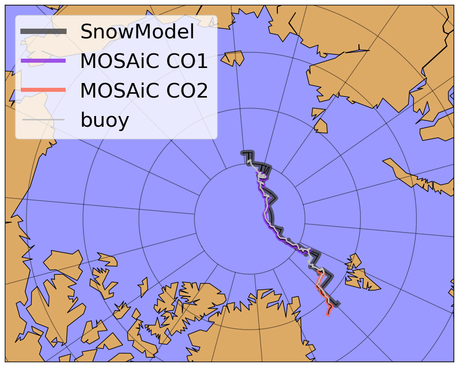
Figure 1 The drift of the Multidisciplinary drifting Observatory for the Study of Arctic Climate (MOSAiC) from October 2019 through July 2020. The first observatory (CO1) lasted from October to breakup in May. The second observatory (CO2) was established in June and July. Autonomous buoys (i.e., drifters) recorded the entire drift. The drift path was extended back to 1 August 2019 using 25 km spatial resolution ice motion vectors from the National Snow and Ice Data Center.

MOSAiC collected an unprecedented quantity of high-spatial-resolution snow and sea ice property data over snow and ice covers of various ages (Macfarlane et al., 2023b; Itkin et al., 2023; Oggier et al., 2023b, a; Raphael et al., 2024). Sea ice thickness and snow depth measurements were collected along transect lines approximately 1 km long with measurements made approximately every 7 d during the entire annual cycle of Arctic sea ice cover from freeze-up, through winter, and until the end of melt (Itkin et al., 2023). In addition, a system of distributed snow pit measurements was used to measure snow density and other snow properties approximately every 7 d throughout the year (Macfarlane et al., 2023b). While the measurements were generally collected once a week, late ship arrival, late freeze up of the melt ponds and FYI, crew exchanges, and sporadic weather and sea ice deformation events caused discontinuities in the observation time series of up to 2.5 months. These discontinuities in the observation data time series (generally summarized as late onset, winter and spring fragmentation, and early truncation), limited its use for process studies and upscaling for satellite remote sensing and numerical model applications.

In this study, we use atmosphere, ocean, ice, and snow measurements from the MOSAiC Central Observatory (Itkin et al., 2023; Cox et al., 2023; Matrosov et al., 2022; Macfarlane et al., 2023b) and autonomous instrument measurements in the surrounding MOSAiC Distributed Network (Lei et al., 2022; Rabe et al., 2024) as forcing and assimilation data to drive a collection of one-dimensional, physics-based, data assimilation, mass balance, and thermodynamic snow and sea ice models as part of a process we call data-model fusion (sensu Boelman et al., 2019; Reinking et al., 2022). This data-model fusion methodology was used to fill in multi-week gaps in the MOSAiC snow and ice data time series and increase their observational data frequency from weekly to temporally continuous (3 h time step), covering the full annual cycle.

In addition, previous analyses of MOSAiC snow depth data (Itkin et al., 2023) showed that snow depth on level ice accumulated more slowly than on deformed ice and that occasional decreases in mean snow depth were observed over all sea ice types. The snow and sea ice thicknesses over various ice ages at MOSAiC were similar at the end of the winter. Here, we use physics-based snow and ice models to explain this snow and ice mass balance evolution during the winter snow and ice accumulation period and during the spring and summer snow and ice melt period.

The two basic assumptions of this work are (1) that the spatially and temporally distributed data collected at MOSAiC are of excellent quality and represent the general annual snow and sea ice cycles and (2) that the numerical modeling tools are able to simulate all the important first-order climate and other environmental processes.

2 MOSAiC observation summary

2.1 Sea ice types at MOSAiC

The sea ice cover in the MOSAiC Central Observatory, surrounding the research vessel (RV) Polarstern, was mainly composed of three ice types:

1. Predominantly deformed SYI that survived the summer melt. This ice type had very few level-ice surfaces. The deformed ice (rubble and ridges) was consolidated during the summer melt period into hummocks and old ridges. The ponds that developed on this ice type over summer remained fresh and were not connected to the seawater.

2. Predominantly level and ponded SYI. At the beginning of October, this ice had very little snow cover, and bare surfaces of refrozen melt ponds were visible. Many of the refrozen melt ponds had previously been connected to the ocean and had a salty surface (Macfarlane et al., 2023b). The remaining ice between ponds was “rotten ice” honeycombed by water before freeze-up.

3. Predominantly level FYI that was still forming throughout October (Itkin et al., 2023). As the thinnest and most level-ice type, this ice underwent frequent deformation and was challenging to sample.

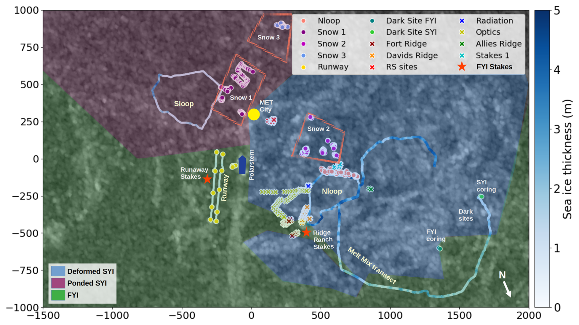
Figure 2 Ice chart with three ice types, transect lines, and point observation sites in the MOSAiC Central Observatory. The transect lines and point sites are all drift-corrected to overlay on the observatory location in October 2019. Transect line ice thickness is displayed in blue shades. Individual snow pit point measurements are marked by symbols, and snow pit polygons are outlined by red dashed lines. The Dark Site, where ice coring activities occurred, MET City, and RV Polarstern location (blue ship-shaped feature at map origin) are also marked. RV Polarstern is located at the origin of the map coordinate system (0,0). The size of the map is 3.5 km by 2.0 km, with distances (m) from the origin marked on the edge of the map. The ship's heading in October 2019 (approximately south-southwest) determines the map orientation. The north arrow shows true north in October 2019. The background is a RADARSAT-2 SAR image from 31 December 2019 (© raw data CSA 2019, provided by NSC/KSAT 2020). The brighter features on the RADARSAT-2 image correspond to deformed ice and SYI. Darker features are level SYI and FYI.

The exact spatial distribution of these three ice types is not known, but based on ground measurements, visual observations, airborne maps, and satellite images, we reconstructed the ice chart of the MOSAiC observatory shown in Fig. 2.

2.2 Observation transects

Snow depth and sea ice thickness data collected along repeated transect lines at MOSAiC were designed to cover diverse ice surfaces that represented large areas of different snow and ice characteristics (Itkin et al., 2023). These repeated, long-transect measurements provided statistically significant snow and ice property datasets over each of the three main MOSAiC ice types and were specifically prioritized over point-wise, but temporally continuous, sampling provided by individual or by clusters of autonomous instruments as in, e.g., Lei et al. (2022), Perovich et al. (2023), Raphael et al. (2024), and Salganik et al. (2023b). They are also superior to large-scale helicopter transects which are generally not repeated over the same sea ice, can be sporadic, and cannot distinguish between snow and sea ice thickness (von Albedyll et al., 2022).

The transects were sampled over all three ice types listed in the section above. These transects are called Nloop, Sloop, and Runway (Fig. 2)

1. Nloop: representing predominantly deformed SYI. This transect was approximately 1.5 km long and sampled between the second half of October 2019 and the beginning of May 2020.

2. Sloop: representing predominantly level and ponded SYI. This transect was approximately 1.5 km long and sampled between the end of October 2019 and the beginning of May 2020.

3. Runway: representing level FYI. This transect was approximately 1.0 km long. This transect was sampled only 3 times in January and February 2020. Afterward, it was not accessible and was partially destroyed by ice motion.

In May the sampling along these wintertime transects was discontinued and in mid-June a new Melt Mix transect (Fig. 2) was established. Part of Nloop and the surrounding FYI were integrated into this new line, but the majority of the ice surfaces were deformed ice. This transect was approximately 3.0 km long and represented all ice types.

2.3 Point observation sites

In addition to transects, this paper relies on ice thickness, snow depth, snow structure, sea ice deformation, ocean heat fluxes, and meteorological data measured at individual point observation sites in the MOSAiC Central Observatory and surrounding Distributed Network (Nicolaus et al., 2022; Rabe et al., 2024).

The Dark Sites (“Dark Site SYI” and “Dark Site FYI”, Fig. 2) were ice coring sites where ice thickness and snow depth were measured regularly between October and July (Evgenii Salganik, personal communication, 2024 and Oggier et al., 2023b, a). The location of these sites was chosen on level SYI and FYI away from the ship to avoid any light or chemical pollution. The FYI at the Dark Site was formed during freeze-up around 1 October and, as such, was a few weeks older than the Runway FYI. Ice coring is a destructive measurement, so the same ice can only be sampled once and the next sample is taken a few meters away. Although only level ice was supposed to be sampled, some samples contained deformed ice that transiently increased the measure of sea ice thickness. At these sites, the ice surface was level and the snow depth was not affected by the vicinity of ridges, yet the number of samples was small and exhibited some variability due to snow bedforms.

In addition, repeated (non-destructive) measurements over exactly the same snow and ice were taken at snow stake and ice hot wire clusters (Raphael et al., 2024). These clusters were relatively small (approximately 10 stakes); herein we only use two stake clusters on the level FYI to augment the low quantity of transect data over this ice type. The two stake sites we used were “Ridge Ranch Stakes” deployed in January close to Fort Ridge and “RunAway Stakes” deployed in February at the Runway (Fig. 2).

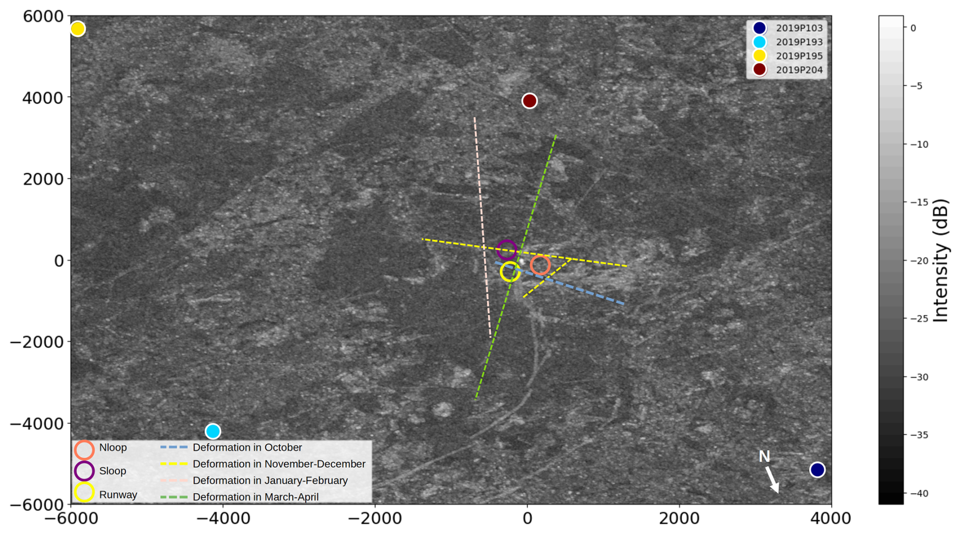
Figure 3 Broader MOSAiC area sea ice cover, GPS buoys, and deformation zones in the vicinity of the Central Observatory. The 4 GPS buoys were at approximately 4–5 km distance from the RV Polarstern (at the map origin). Also shown are the Nloop, Sloop, and Runway transects near the origin. Dashed lines show the approximate location of lead and pressure ridge (deformation) areas in October, November–December, January–February, and March–April. The background is the same RADARSAT-2 SAR image from 31 December 2019 used in Fig. 2 (© raw data CSA 2019, provided by NSC/KSAT 2020.)

Inside the MOSAiC Central Observatory, as well in the Distributed Network surrounding it, 210 autonomous buoys (drifters) were deployed (Rabe et al., 2024; Bliss et al., 2023). While the majority of these buoys were deployed on level sea ice that was stable at their deployment time in October (thick SYI), the sea ice between them was composed of all three ice types described in the section above. A subset of these buoys, 4 buoys transmitting a GPS signal throughout October to May, and forming a square with sides of approximately 5 km (Fig. 3), were used to estimate sea ice deformation. In addition, a selection of 23 buoys within a radius of about 15 km from the RV Polarstern, equipped with thermistor chain measuring snow and sea ice temperature, were used to estimate heat fluxes at the ice–ocean interface (Lei et al., 2022). This network included three L-Sites that were 10 to 20 km from the Central Observatory, where some snow pits were dug with assistance from the helicopter landings throughout the MOSAiC drift (Macfarlane et al., 2023b).

The snow pit sampling sites at MOSAiC were distributed over all three sea ice types (Fig. 2; Macfarlane et al., 2023b). Within these ice types, the majority of the snow pits were dug and measured on level ice, while some sites were in ridges. Similar to ice coring, these measurements are destructive, and every subsequent pit was dug meters away from the previous one and potentially in a different relative position inside a snow bedform. The snow pit locations representative of each of the ice types in the section above were

1. Deformed SYI: Nloop, Dark Site SYI, Fort Ridge, David's Ridge, Allies Ridge, and L Sites.

2. Level and ponded SYI: Snow 1, Snow 2, Snow 3, and RS Sites.

3. Level FYI: Runway, Stakes 1, Dark Site FYI, and partially Optics and Radiation.

Temperature, relative humidity, wind observations used in this paper were collected at METCity on a meteorological tower (Fig. 2) at 10 m height (Cox et al., 2023). Precipitation was measured by the precipitation radar on RV Polarstern (Matrosov et al., 2022).

3 Observations used

3.1 Ship location data

MOSAiC Central Observatory location data were obtained from autonomous buoy 2019I3 (Bliss et al., 2023). To perform our year-long snow and ice simulation, we required ice parcel location information during the entire simulation year (1 August 2019 through 31 July 2020). Only then could the atmospheric reanalysis data be extracted. To define location coordinates prior to October (first 70 d of simulation), a back-trajectory model (Liston et al., 2018) was implemented and driven with 25 km spatial resolution ice motion vectors from the National Snow and Ice Data Center (Tschudi et al., 2020). We identified the ice parcel the ship was anchored to and traced it backwards in time to identify the likely ice parcel location history prior to establishing the observatory. Similarly, ice parcel location data were used to provide ice location data after the buoy malfunctioned in late July (last 7 d of simulation). These procedures resulted in a full-year time series of ice parcel location data (longitude, latitude, and date) that corresponded to the drift of the observatory. As shown in Fig. 1, all used drift trajectories coincide well with each other and the reanalysis data are the same for all trajectories.

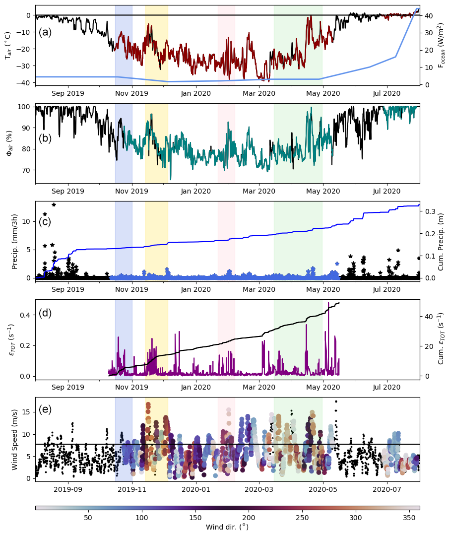
Figure 4 Atmospheric (10 m) and ocean forcing from MOSAiC observations and reanalysis data together with the sea ice deformation data from buoys: (a) air temperature and ocean surface heat flux, (b) relative humidity, (c) precipitation rates and cumulative precipitation, (d) total sea ice deformation ϵ_TOT and cumulative ϵ_TOT, and (e) wind speed and direction. Highlighted by color shading are the periods of storms and increased sea ice deformation. The black values in the plots show missing values filled in by the adjusted reanalysis.

3.2 Atmospheric data

To drive our model simulations, we used 10 m meteorological observations (air temperature, relative humidity, and wind speed and direction) from the MetCity tower (Fig. 2) provided by Cox et al. (2023) and precipitation data from KAZR radar (Matrosov et al., 2022) on board the RV Polarstern. Any gaps in the observational data were filled using bias-corrected NASA Modern Era Retrospective-Analysis for Research and Applications, Version 2 (MERRA-2; Gelaro et al., 2017) reanalysis data. Following standard SnowModel-LG procedures (Liston et al., 2020), the ice parcel coordinate data (longitude, latitude, and date) described above were used to identify the nearest MERRA-2 grid cell that the MOSAiC ice parcel corresponded to on each day of the simulation year. This yielded a full year of meteorological forcing data, with no missing values (Fig. 4). All of the MetCity, KAZR, and MERRA-2 data were then aggregated to 3-hourly values used in the model assimilations (averages for air temperature, relative humidity, and wind speed and direction, and sums for total precipitation). MicroMet was used to distinguish between snowfall and rainfall using the air temperature formulation of Dai (2008) as described in Liston et al. (2020).

Table 1 Bias correction factors were applied (added or multiplied) to MERRA-2 weather data during times when local meteorological observations were not available.

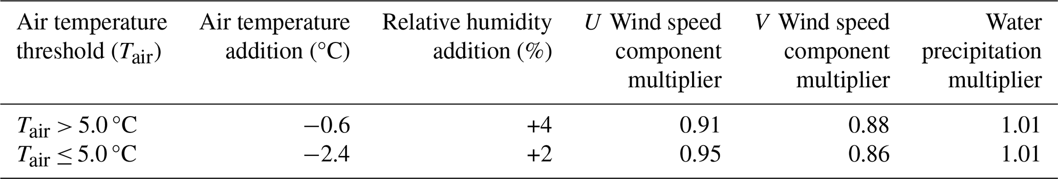
The biases (offsets for air temperature and relative humidity and multipliers for the U and V wind components and precipitation) for each of the atmospheric variables were determined by comparing the averages of the observational and reanalysis data during time periods when both were available. Separate corrections were made for times when the air temperature was above or below −5.0 °C. Periods with air temperatures above this threshold were approximately 1 August–15 September 2019 and 15 May–31 July 2020. For precipitation, we performed the precipitation drizzle adjustment described in Liston et al. (2020) following the trace precipitation analysis of Boisvert et al. (2018). In this procedure, the daily clipping threshold was set to 0.15 mm 3 h⁻¹ (1.2 mm d⁻¹) to create discrete, storm-related precipitation events. Then the clipped precipitation was added to the remaining nonzero precipitation periods, thus conserving the total, temporally integrated MERRA-2 precipitation quantities. The resulting precipitation time series was then bias-corrected using the KAZR precipitation observations. The bias corrections are provided in Table 1.

All the 10 m meteorological observations described above were used as forcing in the MicroMet high-resolution atmosphere model (Liston and Elder, 2006b). The MicroMet simulations also generated additional atmospheric forcing data, including cloud cover, incoming solar radiation, incoming longwave radiation, and surface pressure.

3.3 Initial sea ice thickness and snow accumulation onset

Because the MOSAiC observations started after some sea ice had formed, we defined the initial sea ice thickness and snow accumulation dates based on the bias-corrected reanalysis air temperatures (see Sect. 3.2) and qualitative information from analysis of panoramic photography from MOSAiC during October (Itkin et al., 2023). We assumed the following:

1. Predominantly deformed SYI was 0.5 m thick on 1 August. This ice thickness was estimated based on the modal sea ice thickness in October. Historical summer deployments of ice mass balance buoys show that the ice that survived the summer melt did not start growing before October and that the sea ice thickness in October is a good estimate of the end-of-summer sea ice thickness (e.g., Planck et al., 2020). Snow started accumulating on this ice surface when air temperatures were continuously below freezing, assuming that snow accumulation on melting ice is transient. Based on the 10 m air temperature from reanalysis, and assuming the ice surface may have been melting when air temperatures were above −0.1 °C, the likely surface freeze-up date was 18 August 2020 (Fig. 5). The snow cover appeared thick at the beginning of October (Itkin et al., 2023).

2. Predominantly level and ponded SYI was 0.1 m thick on 30 August. This ice thickness was estimated based on the zero thickness in the melt ponds and the ice content of the rotten ice (modal thickness approximately 0.3 m at the end of October). After 30 August, the 3 d running mean of air temperatures remained below −1.9 °C (Fig. 5), the melted-through melt ponds with seawater in them (Macfarlane et al., 2023b), and the correspondingly low freezing point likely began to freeze, and snow started to accumulate. The 3 d running mean is used here to take into account the heat capacity of the freezing water column, as opposed to freezing the ice surface. The snow cover was thin enough that dark refrozen pond surfaces were still visible at the beginning of October (Itkin et al., 2023).

3. Predominantly level FYI was initiated with 0.05 m thickness (minimum sea ice thickness allowed by the numerical model) on 20 October. The formation of the FYI at the Runway was observed from panoramic photography (Itkin et al., 2023).

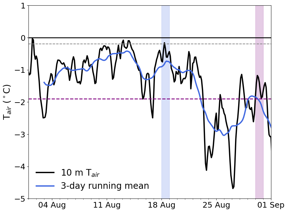
Figure 5 10 m air temperature from bias-corrected reanalysis from 1 August through 1 September 2019 with a 3 d running mean. The date when air temperature departs continuously from the freezing temperature of water is identified by a blue vertical bar. The date when the air temperature running mean departs continuously from the sea ice freezing point is identified by a purple vertical bar.

3.4 Snow depth and ice thickness

At MOSAiC, snow depth measurements along the transects were collected using an automated snow depth probe, Magnaprobe, by SnowHydro LLC (Sturm and Holmgren, 2018). The spacing interval of the snow depth measurements was 1 to 3 m. The distance from the snow surface to the ice–ocean interface (total snow and ice thickness) was measured using a Geophex Ltd., GEM-2 broadband electromagnetic induction device (Hunkeler et al., 2015). The estimated precision of such measurements is approximately 0.1 m. The sea ice thickness was then calculated by subtracting gridded versions of the Magnaprobe snow depth and total snow and ice thickness measurements (Itkin et al., 2023).

For all transects, the level sea ice thickness was estimated from the mode of the ice thickness distribution as in Itkin et al. (2023). To estimate the snow depth on level ice, we averaged the snow depth from all sea ice measurement points where the sea ice thickness was within 0.01 m of the modal sea ice thickness. Depending on the transect, 100–500 measurements were used in the calculations.

The snow depth measurements at the coring site were read from a graded snow stake. Typically, one representative snow depth measurement per ice core was taken, and three ice cores were sampled during each approximately biweekly measurement cycle. Sea ice thickness at the coring sites was measured from the core sampling hole drilled through the ice. Large deviations in sea ice thickness (larger than 1 m from other measurements) were labeled as deformed ice and removed from the analysis.

The snow depth at the stake field was read from snow stakes. The stakes were installed in lines, or grids, approximately 5 m apart. The stakes were initially paired with hot wires (Raphael et al., 2024), but during the winter many wires were lost.

Because during ice melt the ice surface is soft and granular, any stake measurements (including Magnaprobe) can erroneously detect melted ice surfaces as snow after melt onset (Webster et al., 2022; Itkin et al., 2023). Therefore, no snow depth measurements were used after mid-July 2020.

3.5 Snow density

Snow density at MOSAiC was measured in the snow pits by three different methods: (1) by density cutters, (2) by SnowMicropenetrometer (SMP), and (3) by snow core sampler. All three snow density measurements have their advantages and disadvantages. The measurements using density cutters are the most precise but also the most labor intensive. Taylor–LaChapelle density cutters of 3 cm height and 100 m³ volume were used. The density was sampled at 3 cm intervals, covering the entire snow depth profile. All these cutter measurements were then used to calculate the bulk snow density. A total of 243 bulk snow density measurements from cutters were selected from the MOSAiC database (Macfarlane et al., 2023b) to represent the three ice types.

The advantages of the SMP measurements are that they are fast and can efficiently increase the measurement spatial distribution. The SMP measures the force needed to penetrate through the snow depth profile. These force measurements are directly related to snow hardness and can be correlated to snow density (King et al., 2020). It is known (Sturm et al., 2002b), however, that the snow density also depends on the snow texture (grain size, shape, and bonding), and density estimates of large-grained depth hoar can be overestimated when approximated using SMP hardness measurements (King et al., 2020). The SMP density profiles were also used to calculate the bulk snow density (Wagner et al., 2022). In this study, we used 182 SMP measurement sites. Each of these sites was represented by an averaged value for a cluster of five to dozens of distributed measurements at a given location or transect.

Of all three methods, snow core samplers are the fastest and easiest to use. A snow core sampler with a 9 cm diameter was used to sample a vertical column of snow for total snowpack snow water equivalent (SWE). In addition, snow depth was measured, and bulk snow density was estimated directly from these two measurements. The snow core sampler bulk snow density measurements are known to misrepresent the density of a snow cover with large depth hoar crystals, because the depth hoar can collapse during the measurement (López-Moreno et al., 2020). Here we used 166 snow core sampler measurements.

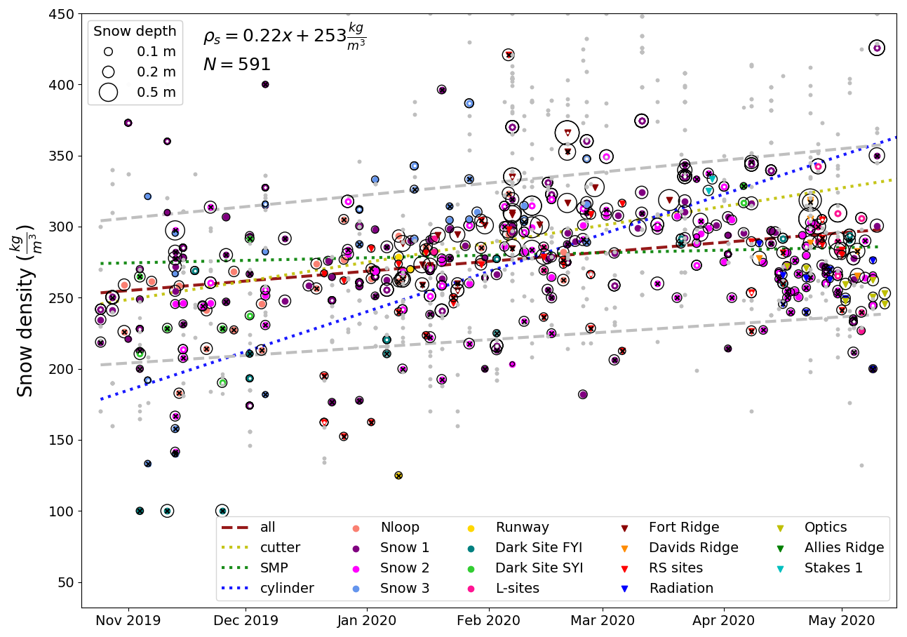
Figure 6 Bulk snow density from density cutters (N=243), SnowMicropenetrometer (SMP, N=182), and snow core sampler (N=166), during the pre-melt period from MOSAiC snow pits. The red dashed line is a linear fit to all the data and the gray dashed lines are the limits of the lower and upper 20 % values typical for depth hoar and wind slab. The yellow, blue, and green lines represent the best linear fits for individual measurement subsets. Estimates from the snow core sampler are identified by a black cross. Estimates from cutters are shown with a white dot. Individual cutter values are displayed as small gray dots.

For the study described herein, the snow density observations described above were used to produce a seamless annual evolution (in a mean, representative in space and time fashion) of bulk snow density over the MOSAiC Central Observatory. To do this, we approximated the annual snow cover snow density evolution (Fig. 6) by fitting a straight line through the data

$$\begin{array}{}\text{(1)}& {\mathit{\rho }}_{\mathrm{s}}=\mathrm{0.22}x+\mathrm{253},\end{array}$$

where ρ_s (kg m⁻³) is snow density and x is time in units of days since 25 October 2019. As pointed out elsewhere (e.g., Sturm et al., 2002a), the snow densification process is generally slow. The increase of density by approximately 50 kg m⁻³ between October and May, shown in Fig. 6, is relatively small compared to the approximately 100 to 150 kg m⁻³ density variability found at and between the sampling locations, at any given time. The MOSAiC bulk density is seemingly independent of the ice type, as found previously for winter snowpacks (Sturm et al., 2002a; Merkouriadi et al., 2017). In contrast, King et al. (2020) found more depth hoar on topographically variable multi-year ice than on relatively smooth FYI. The MOSAiC situation may be explained by the relatively thin snowpack that is similar for all ice types already by early winter (Itkin et al., 2023).

The seasonal development of bulk snow density episodically deviated from this linear fit. For example, the bulk density is lowest after the snowfall events in December and March–May. While the decrease in December is short and transient, the decrease in March–May is long and prominent in the data. This decrease may be a consequence of a sampling bias towards level ice (Fig. 6). The logistical challenges connected to sea ice deformation, in that part of MOSAiC, limited the snow density sampling to the measurement locations at the starboard side of the ship, where only level-ice sites on SYI were sampled. During spring, Snow 1, Snow 2, and many other locations were rarely accessible. The final sampling on Snow 1 provided deeper and denser snow values coinciding with the linear fit. If these were real fluctuations in snow density, they would cause, for the same SWE values, about a 10 % increase in snow depth and correspondingly lower thermal conductivity, further impeding ice growth on all ice types. The amount, scatter, and sampling biases of the data supports our choice of a linear fit; an alternative, higher-degree curve could lead to over-interpretation. A dedicated study of the spatiotemporal development of snow density at MOSAiC is required but is beyond the scope of this paper.

3.6 Sea ice deformation

Hourly location data from 4 GPS buoys (2019P103, 2019P193, 2019P195, and 2019P204; Bliss et al., 2023) within a radius of approximately 5 km from the RV Polarstern (Fig. 3) were used to quantify MOSAiC Central Observatory sea ice deformation. The total sea ice deformation ϵ_TOT (Fig. 4d) was calculated from 3-hourly positions (every third hour was extracted from the hourly data) following Hutchings et al. (2012):

$$\begin{array}{}\text{(2)}& {\mathit{ϵ}}_{\text{TOT}}=\sqrt{{\mathit{ϵ}}_{\text{DIV}}^{\mathrm{2}}+{\mathit{ϵ}}_{\text{SHR}}^{\mathrm{2}}},\end{array}$$

where ϵ_DIV is divergence and ϵ_SHR is shear calculated by line integrals. This general sea ice deformation measure was used to avoid the errors associated with deformation calculations that separate the individual contributions from convergence, divergence, shear, and the associated lead and pressure zone processes (Hutchings et al., 2012; Itkin et al., 2017).

These 4 buoys are a subset of the distributed buoy network deployed at MOSAiC (Nicolaus et al., 2022; Bliss et al., 2023). They were selected because their spacing roughly formed a rectangle throughout the entire period from October through May.

The coarse-resolution sea ice deformation data obtained from the 4 buoys were supplemented by qualitative analyses of relative sea ice motion from ship radar images (Krumpen et al., 2021). The ship radar images cover an area with a radius of 5.4 km around the RV Polarstern and have a spatial resolution of 8 m. These images were collected throughout the MOSAiC expedition every 2 s. For this paper, we analyzed the temporal changes that occurred in hourly animations of these images to detect the approximate timing and locations of major shear zones and lead openings within the approximate 5 km buoy radius of the RV Polarstern.

Based on weather and sea ice deformation data, we determined 4 periods when high winds, snowfall, high deformation rates, and large relative motion in the MOSAiC Central Observatory (Fig. 3) were observed. These periods are marked in Figs. 4, 8, and 9 and will be used to discuss the deformation-associated snow sinks. The periods are

1. October shearing and ridging from 16 October to 1 November: marked by blue shading.

2. November shearing and ridging from 14 November to 5 January: marked by yellow shading.

3. January lead from 22 January to 7 February: marked by pink shading.

4. March–April leads from 15 March to 30 April: marked by green shading.

3.7 Ocean heat flux

Ocean surface heat fluxes used in this study loosely follow the estimates of Lei et al. (2022) based on a cluster of 23 buoys, the “Sea Ice Mass Balance Array” (SIMBA), designed by Jackson et al. (2013). SIMBAs are equipped with thermistor chains that measure temperature through air, snow, ice, and ocean. The time series was extrapolated with constant values to cover the period prior to the buoy deployment (Fig. 4a). At the end of our analyzed period (9–29 July 2020), we adjusted the Lei et al. (2022) time series to increase from 16 to 44 W m⁻². This was based on estimates by Salganik et al. (2023a) using level-ice temperatures and bottom melt rates in the Central Observatory. Several other researchers have used SIMBA or similar data to estimate snow depth and sea ice thickness evolution at MOSAiC (Lei et al., 2022; Perovich et al., 2023; Salganik et al., 2023b).

4 Models used

4.1 SnowModel-LG

In this study, SnowModel was used to represent snow-on-sea-ice processes and evolution. SnowModel has its origins as a terrestrial, multilayer, spatially distributed snow evolution modeling tool (see Liston and Elder (2006a) and the references contained therein). It is coupled to a high-resolution atmospheric model called MicroMet (Liston and Elder, 2006b) that provided surface forcing (based on the 10 m meteorological forcing summarized in Fig. 4) to SnowModel (Liston and Elder, 2006b) and SnowAssim that assimilates available observations (Liston and Hiemstra, 2008). Adaptation of these models to Lagrangian drifting sea ice environments and ice parcels (SnowModel-LG) was described by Liston et al. (2018), Liston et al. (2020), and Mower et al. (2024). In this study, we used a 1-D (vertical profile) version of the multilayer modeling system to create high resolution time series (3 h time increment) of MOSAiC snowpack development and evolution. In SnowModel, the change of SWE with time is calculated by solving the snow source and sink equation

$$\begin{array}{}\text{(3)}& {\displaystyle \frac{\mathrm{d}\text{SWE}}{\mathrm{d}t}}={\displaystyle \frac{\mathrm{1}}{{\mathit{\rho }}_{\mathrm{w}}}}\left[\right(P_{\mathrm{R}}+P_{\mathrm{S}})-(S_{\text{SS}}+S_{\text{BS}}+M)\pm D],\end{array}$$

where SWE is snow water equivalent (m); ρ_w is water density (1000 kg m⁻³); P_R and P_S represent sources of snow cover from rainfall and snowfall; S_SS, S_BS, and M represent the snow cover sinks through static sublimation, blowing snow sublimation, and melt; and dt (s) is the model time increment (= 10 800 s = 3 h in this application). Finally, D represents the sea ice deformation snow sink or source. The units of all sources and sinks are $\mathrm{kg}{\mathrm{m}}^{-\mathrm{2}}{\mathrm{s}}^{-\mathrm{1}}$. Snow depth h_s (m) is estimated as

$$\begin{array}{}\text{(4)}& h_{\mathrm{s}}=\text{SWE}{\displaystyle \frac{{\mathit{\rho }}_{\mathrm{w}}}{{\mathit{\rho }}_{\mathrm{s}}}},\end{array}$$

where ρ_s (kg m⁻³) is snow density.

Because SnowModel-LG operates in SWE, while the MOSAiC observations provide h_s (Sect. 3.4) and ρ_s (Sect. 3.5 and specifically Eq. 1 with continuous values for ρ_s), any comparison can be made using Eq. (4) which determines the relationship between the three variables.

4.2 HIGHTSI

In this study, a 1-D thermodynamic sea ice model called HIGHTSI (Launiainen and Cheng, 1998; Cheng et al., 2008; Merkouriadi et al., 2020) was used to simulate sea ice thickness evolution. In this application, the snowpack used in HIGHTSI was provided by our SnowModel-LG assimilations. In HIGHTSI, the snow thermal conductivity, k_s, was parameterized using the snow density, ρ_s, based on a second-order polynomial fit from MOSAiC snow pit data following Macfarlane et al. (2023a):

$$\begin{array}{}\text{(5)}& k_{\mathrm{s}}=\mathrm{2.62}\times {\mathrm{10}}^{-\mathrm{6}}{\mathit{\rho }}_{\mathrm{s}}^{\mathrm{2}}+\mathrm{1.54}\times {\mathrm{10}}^{-\mathrm{33}}{\mathit{\rho }}_{\mathrm{s}}+\mathrm{3.04}\times {\mathrm{10}}^{-\mathrm{2}}.\end{array}$$

This parameterization resulted in a seasonal bulk snow thermal conductivity increase from 0.21 ${\mathrm{WK}}^{-\mathrm{1}}{\mathrm{m}}^{-\mathrm{1}}$ in October 2019 to 0.27 ${\mathrm{WK}}^{-\mathrm{1}}{\mathrm{m}}^{-\mathrm{1}}$ in May 2020. These values coincided well with estimates of Raphael et al. (2024), who provided an insightful discussion of the quality of the snow thermal conductivity estimates at MOSAiC. The ice thermal conductivity was constant in HIGHTSI throughout the winter and set to 2.03 ${\mathrm{WK}}^{-\mathrm{1}}{\mathrm{m}}^{-\mathrm{1}}$. During the melt period, ice conductivity depended on the surface temperature and salinity. For our HIGHTSI simulations, during melt, it was set to vary between 1.7 and 2.1 ${\mathrm{WK}}^{-\mathrm{1}}{\mathrm{m}}^{-\mathrm{1}}$, following the ice surface conductivity measurements made during MOSAiC (Macfarlane et al., 2023a).

5 Simulations and results

To satisfy our general goal of using a collection of modeling tools (SnowModel-LG and HIGHTSI) to fill in temporal gaps in MOSAiC field observations, we made the following assumptions and performed the following tasks. First, we assumed the MOSAiC field observations were perfect; we made no effort to correct them for any potential measurement errors, as others undertook those tasks (e.g., Cox et al., 2023; Matrosov et al., 2022; Itkin et al., 2023). In addition, we configured our modeling tools to fill data gaps between those observations with modeled values that were as realistic as possible. Our general vision was to produce snow and ice time series information, with no missing data, covering a full snow and ice evolution year at a 3 h time increment, containing MOSAiC snow and ice observations when they existed, and physically realistic values during any periods when they did not.

The procedures described below were implemented for the three ice types described in Sect. 2.1.

5.1 Snow calculations

Our snow simulations began using SnowModel-LG to solve Eq. (3), with the ice dynamics term, D, set to zero, with the atmospheric forcing data described above.

5.1.1 Sea ice deformation snow sink and source calculations

To understand the role of ice deformation, D, in the evolution of snow properties, the difference between modeled and observed SWE was assumed to equal D in Eq. (3) (model minus observed; thus positive D values represent an SWE sink, or an SWE loss resulting from ice dynamics). Then, to create a continuous D time series at the 3 h time increment, D was linearly interpolated between the sea ice freeze-up date (zero snow depth) and individual SWE observation times. Before and after these dates, D was set to zero, under the assumption that no blowing snow occurs when air temperatures are above freezing and the snow may be melting (e.g. Li and Pomeroy, 1997). This D term was then subtracted from the model simulated SWE to create a temporally continuous SWE evolution that matched the SWE observations when they occurred and filled in realistic SWE values during periods of no SWE observations.

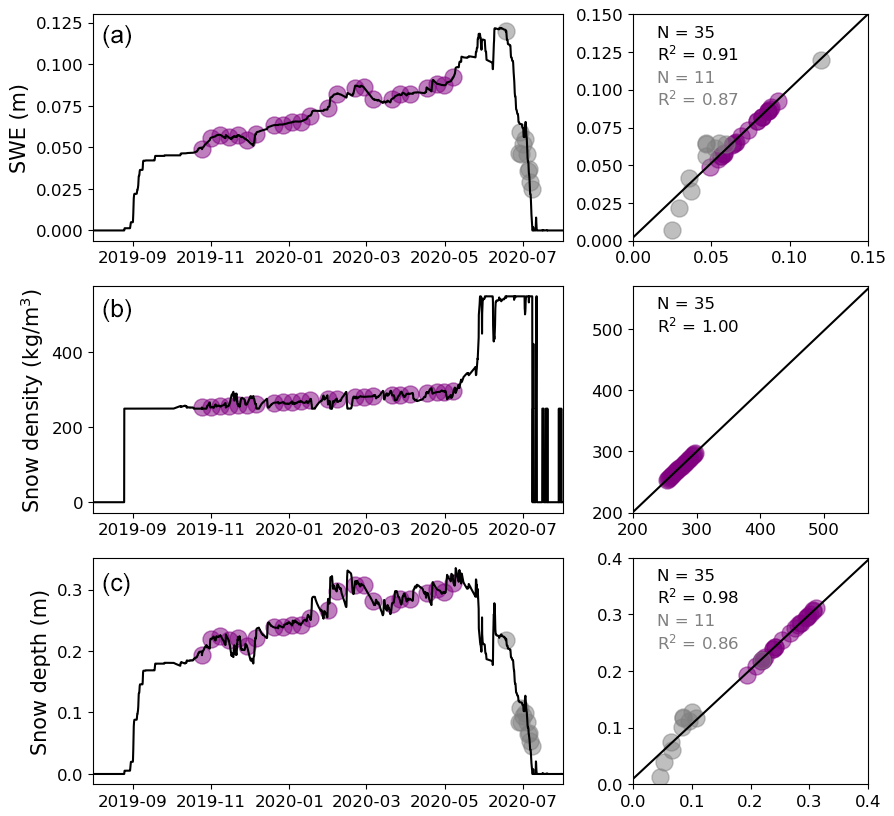
Figure 7 Nloop SnowModel-LG snow assimilation time series and scatter plots (x axis for observations and y axis for model) for (a) SWE, (b) bulk snow density, and (c) snow depth in each of the figure rows. Assimilated observed values are represented by purple circles. Non-assimilated observed values (melt period) are represented by gray circles. In the right column, correlations for all data are printed in black, and correlations for the melt period are written in gray. All correlations are significant.

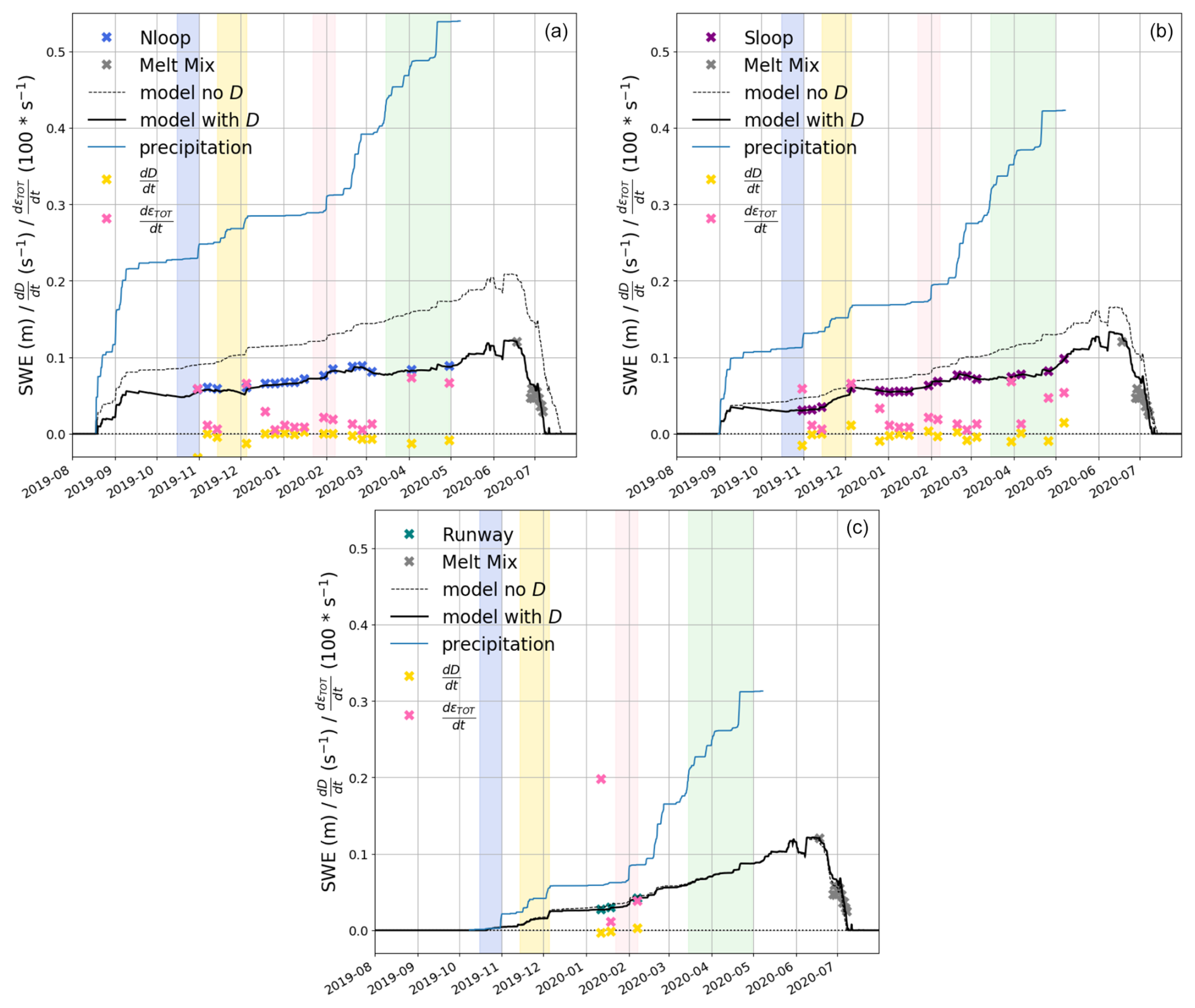
Figure 8 Transect observations and SnowModel-LG simulations of SWE for (a) Nloop, (b) Sloop, and (c) Runway. Input precipitation from snow accumulation onset and time derivatives of D ($\frac{\mathrm{d}D}{\mathrm{d}t}$) and ϵ_TOT ($\frac{\mathrm{d}{\mathit{ϵ}}_{\text{TOT}}}{\mathrm{d}t}$) are also displayed. Highlighted by color shading are the periods of storms and increased sea ice deformation. Signs of $\frac{\mathrm{d}D}{\mathrm{d}t}$ discriminate between source and sink.

Figure 7a presents a comparison of the SWE observations and the simulated SWE time series for the deformed SYI ice type (Nloop transect); the other two ice types are similar and not shown. Figure 8 presents the resulting time evolution of D and SWE for the three types of MOSAiC ice.

5.1.2 Snow depth

To calculate the snow depth evolution, the final SWE evolution defined above was further modified using the MOSAiC snow density observations. Equation (1) was used to define the observed snow density at the SWE observation times. We then calculated the ratio of this observed snow density to the SnowModel-LG-produced snow density at those times. This created a density correction parameter that, when multiplied by the model-simulated snow density, reproduced the observed density. Similar to our SWE adjustments, these correction parameters were linearly interpolated between the observations, with the correction set to unity before the first observation and after the last observation. This correction time series was then multiplied by the model-simulated snow density to create a temporally continuous density evolution that matched the density observations when they occurred and filled in realistic density values during periods with no density observations. Figure 7b presents a comparison of the snow density observations and the simulated density time series for the deformed SYI ice type (Nloop transect); the other two ice types are similar and not shown. There were no density observations taken during the melt period.

Snow depths over the annual simulation period, with 3-hourly time increment, were then created using Eq. (3), with inputs of the 3-hourly SWE and snow density data described above (Fig. 7c).

5.2 Thermodynamic ice growth calculations

The temporally continuous snow depth and density evolution over the three ice types, the atmospheric forcing, and the ice–ocean interface heat fluxes were used to force the HIGHTSI thermodynamic sea ice model. The snow simulated in the previous section represents the mean snow cover, including both snow on level sea ice and snow on deformed ice. Because the modal sea ice thickness only represents level sea ice thickness, and since HIGHTSI only simulates thermodynamical sea ice growth, we performed separate SnowModel-LG simulations over each of the three ice types, assuming level ice only, to create the snow forcing for the HIGHTSI sea ice simulations. This was done by repeating the calculations described in the previous sections while only using SWE observations collected over level, undeformed ice.

In addition, to account for the role of meter-scale snow depth variability resulting from snow bedform (e.g., snow dunes and sastrugi) snow-depth variability found on level ice, 1 standard deviation of snow depth was removed from the simulated level-ice snow. This step effectively accounts for the role that thin snow, in the troughs between the snow bedforms on level ice, has on enhanced ice growth (Sturm et al., 2002b; Liston et al., 2018) and can be thought of as a simple, bedform-scale heat transfer parameterization.

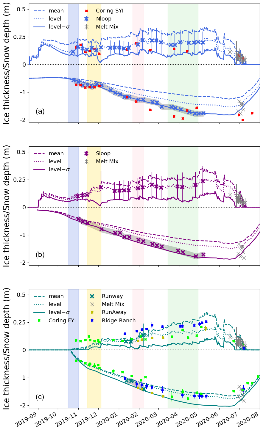
Figure 9 Seasonal development of snow and ice cover from model and observations for (a) Nloop, (b) Sloop, and (c) Runway. Simulations are represented by lines and observations by points. The error bars of observations represent 1 standard deviation. The gray shading around the sea ice thickness modes estimates indicates the 0.1 m precision of the GEM-2 method. Highlighted by color shading are the periods of storms and increased sea ice deformation. The snow depth scale is exaggerated four times compared to sea ice thickness.

Approximately 16 % of all level-ice snow depth measurements along the transects had snow depths at or lower than the mean level-ice snow depth minus 1 standard deviation. This corresponds to the proportion of troughs between the snow bedforms in the MOSAiC snow transect observations. Our simulations used observed MOSAiC snow depths and observed snow and ice thermal conductivity (Macfarlane et al., 2023a) to drive our ice growth simulations. Figure 9 presents the comparison of the ice thickness model simulations and observations for the three types of MOSAiC ice. For each ice type, model simulations with mean snow depth (level and deformed ice), level-ice snow depth, and level ice reduced by 1 standard deviation are presented.

6 Discussion

As demonstrated in over 200 publications, MicroMet, SnowModel, SnowModel-LG, and SnowAssim have been shown to reproduce a wide range of snow-related observations found in terrestrial and sea ice environments around the world (e.g., see the references contained within Liston et al. (2020) as a representative subset of these publications). This study and the analyses presented herein provide four opportunities that are unique compared with those studies: (1) to identify snow and ice processes and evolution that likely took place during the MOSAiC snow and ice evolution year before the ship arrived and during winter, spring, and summer periods when the ship was not stationed in the ice or when snow and ice measurements were not possible for some reason; (2) to help understand and quantify the role of ice dynamics on snow mass budgets; (3) to help understand and quantify the role of the resulting snow distributions on sea ice growth and decay; and (4) to help understand the processes of the early melt season, including estimating the timing of melt onset of snow, the first snow-free date, and melt onset of ice. The following discussion analyzes these four issues.

6.1 Missing time periods during the MOSAiC observation year

Using an atmospheric reanalysis that was bias-corrected by MOSAiC observations, atmospheric observations from the MOSAiC observatory, and extrapolated ocean heat flux estimates, we used SnowModel-LG with assimilated snow observations and HIGHTSI to create a seamless snow and ice property time series with a 3-hourly time step for the entire ice year from 1 August 2019 through 31 July 2020. The model simulations were critical to fill in three kinds of missing data: (1) the time period before the ship's arrival and the start of observations, (2) missing data due to weather and logistical reasons, and (3) times between the regular discrete observations of snow properties and sea ice thickness.

Before the ship's arrival, we used bias-corrected atmospheric reanalysis data to estimate the snow accumulation and freeze-up time for the three ice types (see Sect. 3.3). Although the timing of freeze-up is critical for the snow and ice cover, this period is logistically challenging for any ship-based snow and ice observation expeditions (Nicolaus et al., 2022) or autonomous instrument programs (Rabe et al., 2024). In particular, by the onset of MOSAiC observations, the difference between accumulated snowfall and SWE was already nearly 50 %. Then, occasionally, during winter, the continuous weather data collection or weekly snow and ice sampling was interrupted due to ice break-up, weather, or logistical reasons, such as crew exchanges (Cox et al., 2023; Matrosov et al., 2022; Itkin et al., 2023; Nicolaus et al., 2022). However, the bias-corrected atmospheric reanalyses data were of sufficient quality that SnowModel-LG simulated physically credible values during these missing periods.

Another period without any measurements was between 7 May and 15 June. Still, SnowModel-LG simulated the transient melt onset at the end of May, when the first extensive melt ponds of the season were widely observable on satellite images (Webster et al., 2022). In addition, the model accurately reproduced the first observations collected in June, more than a month after 7 May, when the last snow measurement was assimilated (Fig. 7).

This means that, through the fusion of observational data and numerical models, we successfully bridged the periods when no spatially distributed data were collected at MOSAiC.

The 7 d observation period of the MOSAiC transects was chosen to resolve the synoptic cycle of snow accumulation and ice growth. The data-model fusion we implemented here produced a full-year time series (1 August 2019 through 31 July 2020), at a 3 h time increment that resolves the timing of any atmospheric events with high temporal precision. This is relevant to understanding snow and ice processes, as well as atmosphere–snow–ice–ocean interactions. In addition to the suite of snow and ice related variables presented herein, these simulations come with numerous other surface energy flux and mass balance variables that are all internally consistent with each other; this is a numerical requirement of all the modeling tools used in this study.

6.2 Sea ice deformation can be an important snow source or sink

Previously, Liston et al. (2020) demonstrated that sea ice deformation, calculated as a residual using coarse-resolution atmospheric and ice concentration and movement forcing data at the pan-Arctic scale, was highly correlated to the sea ice drift and the new ice formation associated with it. In this study, we extend their findings to a local scale by examining the connection between the snow mass balance term (herein formulated as D; see Eq. 3) and sea ice deformation (Eq. 2). Using observed and estimated atmospheric forcing data and periodic SWE and snow density observations, SnowModel-LG simulated physically credible snow evolution on the three sea ice types with different ages and sea ice deformation characteristics found at MOSAiC (Fig. 8).

On all three ice types, the strongest winter season sinks in our simulations were static and blowing snow sublimation (S_SS and S_BS), which, by 7 May, cumulatively removed 67 %, 68 %, and 71 % of SWE from snowfall (P_S) in Nloop, Sloop, and Runway, respectively. This is represented by the difference between “precipitation” and “model no D” in Fig. 8. The magnitude of S_SS and S_BS depends on grain bonding, which is, for S_SS, determined by latent heat flux, while for S_BS, wind speed, humidity, and solar radiation are the main factors (Liston et al., 2020). Note that, in this environment, if the blowing snow is not captured by an ice-topographic drift trap or blown into an open lead, it blows perpetually, and, in air that has a humidity deficit, it eventually sublimates completely away (Tabler, 1975; Liston and Sturm, 2004). These S_SS and S_BS values were about 3 times as large as in Liston et al. (2020). This is likely due to the specific weather during MOSAiC winter and location during the drift, including generally low snowfall (P_S) after freeze-up, frequent storms with high winds (Rinke et al., 2021), and relatively high sea ice concentration (Krumpen et al., 2021) with low near-surface relative humidity during winter. P_S, S_SS, and S_BS operate at synoptic temporal and length scales (on scales comparable to, e.g., 3 h and 100 km) and were the same (or very similar for S_SS and S_BS) for all ice types.

The differences in SWE evolution on the three ice types were largely controlled by the ice (and snow) onset date and the differences in the remaining wintertime snow sink or source – the ice dynamics term D. These factors operate at much shorter local spatial scales, e.g., 10 m. This is represented by the difference between “model no D” and “model with D” in Fig. 8. D is the only local simulated source or sink; in the natural system, D produces ice roughness features such as rubble ice and pressure ridges, as well as lead timing, size, and distribution. Following any sea ice deformation, a certain amount of airborne snow will be removed to open water in the leads (Clemens-Sewall et al., 2022) or stored in snowdrifts at the deformed ice roughness features (Liston et al., 2018; Itkin et al., 2023). During winter, the wind velocity is frequently above the blowing threshold value (7.7 m s⁻¹) following Li and Pomeroy (1997), which provides the justification for our parameterization of D as a sea ice deformation snow sink or source (see Sect. 5.1). After melt onset, the snow grains are wet, and no drifting snow is observed (sensu Pomeroy et al., 1997). Following this principle, D was set to zero in May after the last transect measurements.

D remained small throughout the simulations, but its accumulated effect by 7 May (the last winter observation) was 15 %, 8 %, and < 1 % in Nloop, Sloop, and Runway, respectively. D is likely large right after freeze-up; this is a period of thin ice with frequent deformation. More studies of this fast-changing period with thin ice are needed to understand what exactly is happening when the ice first forms. The importance of erosion for SWE at MOSAiC was explored by Wagner et al. (2022), who gave estimates of erosion based on uncalibrated snowfall rates, wind speeds, and SWE in Sloop and Nloop. While the magnitude of the combined snow sink by Wagner et al. (2022) is similar to ours (53 %–68 %), their study could not differentiate between erosion–deposition and sublimation. Our study shows that D was predominantly a sink (erosion) in the case of Nloop and Runway and, after ridge formation in November, was occasionally a source (deposition) in Sloop.

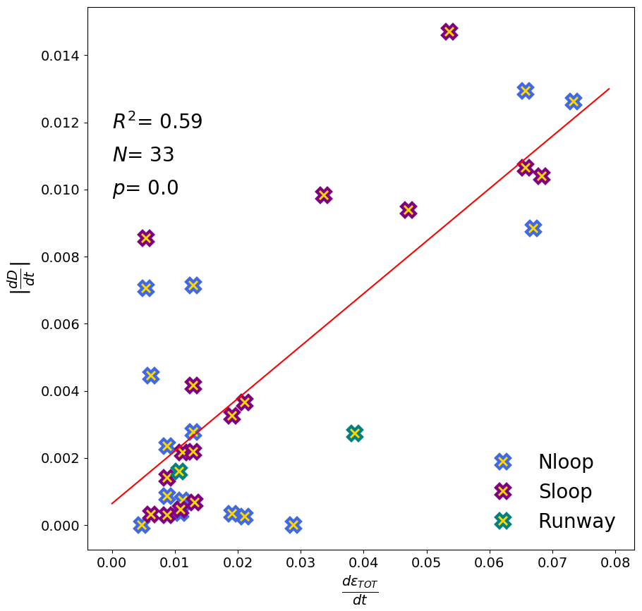
Figure 10 Scatter plot of derivatives of D and the cumulative total deformation. The time steps between observations in Nloop and Sloop are the same (with some observations during quiescent periods are skipped in Nloop, which had more frequent observations than Sloop).

Strong winds are generally associated with synoptic events that often cause sea ice deformation and bring precipitation. For Sloop, high wind speeds had no significant statistical correlation with the time derivative of D, but we found a strong (R² = 67 %, N=16, p=0.0001) linear correlation between the absolute value of this derivative and the derivative in accumulated total sea ice deformation – ϵ_TOT estimated from the GPS buoys (see Sect. 3.6). Nloop development can be calculated over 23 derivatives, with 8 giving meaningless rates falling between two consecutive deformation events and simply showing no change during quiescent periods. Instead, those redundant steps and their derivatives were removed from calculations in this analysis. When using similar derivatives over sampling steps in time as for Sloop, the correlation was similarly strong (R² = 62 %, N=15, p=0.0016). For Runway, the sample size was too small (N=2) to perform this analysis, but a combined analysis for all locations shows a strong correlation as well (R² = 59 %, N=33, p=0.0001, Fig. 10). Note that we used the absolute values of the D derivative, since ϵ_TOT is also spatially averaged, and differentiation between sink and source is not possible with these data.

This analysis was only possible because the MOSAiC precipitation observations have sufficiently low errors that a minor signal such as snow redistribution due to sea ice deformation could be detected. This was, in turn, also only possible because the in situ transect and sea ice deformation observations were frequent enough to resolve the synoptic cycle's contributions to snow and ice evolution.

To understand the reasons for these statistical correlations, we tracked the timing and location of major leads and pressure ridges (Fig. 3) occurring in the vicinity of the MOSAiC transects on the ship radar images (see Sect. 3.6) during periods of increased winds, snowfall, and high deformation rates (Figs. 4 and 8). Such qualitative analyses allowed us to distinguish between the sink and source direction of D. We found that any close-upwind deformation was associated with an SWE decrease. Any deformation inside the transect, or just adjacent to it, was connected to an SWE increase that could not be explained solely by snowfall. For example, in late October and November, pressure ridges formed north of Nloop (blue line in Fig. 3). This was accompanied by SE winds that accumulated snow in Nloop—just some 100 m upwind of the new ridges. In November and December, a new lead and ridge line were created between Sloop and Nloop (yellow line in Fig. 3). This time, the winds were strongly SW. Nloop was upwind, and a new ridge formed inside Sloop. Sloop gained SWE, and Nloop lost it. At the end of January and beginning of February, a lead was active east of Sloop (pink line in Fig. 3). The W winds first caused a local source of snow in Sloop. When winds turned to E, the lead was the local sink that caught snow and prevented deposition in Sloop. Nloop was too far away to be affected. In March and April, a large lead separated Nloop and Sloop once again (green line in Fig. 3). The winds were mainly S along the lead but with occasional W winds. The upwind Sloop lost a considerable amount of snow. Because the winds were E in May, Sloop again gained some snow during this time. Nloop was further away from the deformation zone and mainly lost snow during this period as well.

The strong correlation between derivatives of D and ϵ_TOT for these major deformation events strongly suggests that there was an immediate response to the creation of new roughness elements and open water areas. This is in contrast to the slow accumulation occurring in the old roughness features created during previous deformation events. Spatially distributed, 3-dimensional simulations, similar to those performed by Liston et al. (2018), over a dynamic topography that quantifies sea ice deformation at much higher resolution than a handful of GPS buoys, are necessary to estimate how much snow is stored on new rough ice, how much is lost to open water, and how much sublimates away. Such a study would also be able to confirm or reject a recent observational study, based on spatially very constrained MOSAiC ice core data in refrozen leads (N=5), that indicated very little snow was lost to leads (Clemens-Sewall et al., 2022). Liston et al. (2020) presented a list of eight reasons why snow blowing into leads is likely a minimal component of the snow-on-sea-ice moisture budget. In contrast, loss of snow into leads is used as a tuning parameter in some climate model simulations (Petty et al., 2018; Schröder et al., 2019).

The large magnitude of D in Nloop may be a peculiarity of MOSAiC. The MOSAiC snowpack was thinner than the climatological mean (Itkin et al., 2023), and snowdrifts in pressure ridges and deformed ice can store all snow volume if there is very little snow. This is a known phenomenon well researched in terrestrial systems (e.g., Tabler, 1975; Benson and Sturm, 1993; Sturm et al., 2001; Liston et al., 2016, 2025). In windy environments with little snow, all snow will be trapped in the ridges or other ice-surface roughness features. Over the course of the winter, the fraction of snow volume in topographic drift traps should decrease as the trap fills to capacity and the snow depth in other (non-snowdrift-trapping) areas increases. At MOSAiC, this never happened because there was very little snow and newly deformed ice was frequently created. As evidence of this, the snow depth standard deviation in the pressure ridges increased throughout the winter, because they were never completely filled to their maximum snow-holding capacity (Itkin et al., 2023).

The SWE on all ice types was different at the start of the MOSAiC observations, but it became increasingly similar towards the end of the snow accumulation season. Since all three ice types were adjacent to each other and part of the same turbulent wind field, air temperature conditions, and precipitation forcing, some snow appears to be transported from the oldest and least dynamic ice type (Nloop) to the most dynamic (Sloop) and youngest (Runway) ice types. This is another hypothesis that could be explored by high-resolution, spatially distributed simulations that cover various sea ice types with different ice roughness characteristics. Such a study would benefit from some kind of snow particle transport accounting within the modeling system that would identify and quantify the origins and deposition locations of snow particles being redistributed by the wind.

6.3 Impact of snow on sea ice growth

As already shown by Itkin et al. (2023) and Raphael et al. (2024), younger and thinner sea ice types at MOSAiC with initially thinner snow (Sloop and Runway) had faster sea ice growth rates early in the growth season than the oldest sea ice type with initially deeper snow (Nloop). Similar findings have been demonstrated in previous observational (Sturm et al., 2002a; Provost et al., 2017; Rösel et al., 2018) and modeling studies (e.g., Notz, 2009). At MOSAiC, the relatively low initial sea ice thickness of the SYI (Sect. 2.1) and the differences in growth rates led to FYI sea ice thicknesses that were approximately equal to that of the SYI by as early as mid-November 2019 (Fig. 9).

The importance of the snow accumulation onset for ice growth and spring sea ice thickness is visible even for various ages of FYI (Fig. 9c). There were two ages of FYI that were sampled at MOSAiC. The FYI at the coring site was formed at freeze-up, on about 1 September, and accumulated practically the same amount of snow as Sloop. This is also the FYI onset date used by von Albedyll et al. (2022) in a large-scale MOSAiC study. The Runway and Fort Ridge FYI formed about a month later in leads, and they missed the snowfall during that period. The Ridge Ranch stakes at the Fort Ridge were close to a ridge and accumulated snow the fastest. The FYI with the thinnest snow grew the thickest by the end of winter. This is visible in the observations (May) and the model simulation and suggests that the variability of the level FYI thickness can be larger than the variability of the level SYI thickness.

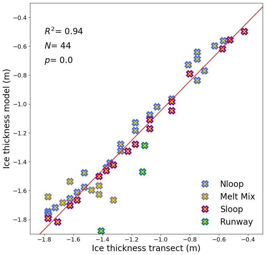
Figure 11 Scatter plot of modal sea ice thickness from transect observations and simulated sea ice thickness. The linear correlation coefficients are estimated only for the winter transects (Nloop, Sloop, and Runway).

The high correlation (R² = 0.94, N=44) of simulated and observed winter sea ice thickness (Fig. 11) is clear evidence of the importance of the local snow depth and density for ice growth. Besides these two local variables simulated by SnowModel-LG, HIGHTSI was also forced by atmospheric temperature (Sect. 3.2) and ocean heat fluxes (Sect. 3.7) that were assumed uniform for all MOSAiC ice types. In addition, two storms increased the snow-depth variability at MOSAiC: (1) the November storm (yellow shading in Fig. 9) increased the standard variability in Nloop and Sloop, and (2) the January–February storm (pink shading in Fig. 9) increased the standard variability on Runway. Both events were followed by an increase in level-ice thickness. This indicates that the developed snow bedforms promote loss of heat from the ocean and highlights the relative importance that local-scale (locally one-dimensional or fully three-dimensional) heat fluxes, through the snow and sea ice, play in governing ice growth (as suggested by Sturm et al., 2002b, Liston et al., 2018, and Itkin et al., 2023).

Our bedform parameterization (using the level-ice mean snow depth minus 1 standard deviation as described in Sect. 5.2) is an example of how these local-scale, sub-grid phenomena and processes can be accounted for in climate system models in order to accurately reproduce observed sea ice growth. Instead, current climate models often use thermal conductivity values that are approximately 50 % larger than those measured (Macfarlane et al., 2023a; Raphael et al., 2024) and used here (Eq. 5), effectively increasing the heat transfer through the snow in an effort to reproduce observed ice growth. The results presented herein suggest that climate system models need to account for local-scale heat transfers instead of adjusting the snow thermal conductivity away from observed values. Sturm et al. (2002b) also came to this conclusion over two decades ago. Spatially distributed, 3-dimensional simulations of snow and sea ice are necessary to study the heat fluxes and local consequences of snow for sea ice growth.

The ocean surface heat fluxes during winter were low (Fig. 4a), and the ocean surface was very cold or even supercooled (Katlein et al., 2020). During this time, the ice growth was mainly governed by low atmospheric temperatures and snow thermal conductivity.

Our estimates of initial thickness and snow accumulation onset dates (Sect. 3.3) are unfortunately crude. More observations from that period, in addition to distributed model runs, may provide better insights into snow and ice initiation and evolution during that period. Another weakness of the MOSAIC dataset is the lack of repeated transects on the FYI (as discussed in Sects. 2.2 and 2.3). The data from the coring sites and stakes are not directly comparable to the transect location (see also discussion above) and can not be included in the statistical analysis (Fig. 11).

6.4 Snowmelt and ice melt onset

Snowmelt began while RV Polarstern was not present in the MOSAiC Central Observatory, during the time window between 10 May and 15 June (Nicolaus et al., 2022). Several authors have attempted to estimate this date based on point measurements from buoys with thermistor chains (Lei et al., 2022; Perovich et al., 2023; Salganik et al., 2023b; Raphael et al., 2024) or satellite imagery (Webster et al., 2022). In our simulations, the snow depth started gradually decreasing simultaneously with the snow density increase shortly after the last transect measurement on 7 May (Fig. 7). This coincided with a storm with strong winds and air temperatures near zero (Fig. 4a) and a snow depth decrease detected by thermistor chains (Salganik et al., 2023b). Other thermistor-chain-based studies estimated snowmelt onset at much later dates on 15 May (Lei et al., 2022) and 8 June (Perovich et al., 2023). The air temperatures were positive for the first time with the storm on May 27 (Fig. 4a), coinciding with rainfall (Fig. 4c) and a decrease in both simulated SWE and snow depth (Fig. 7). The simulated density increased abruptly on 27 May and reached its maximum value (550 kg m⁻³) on 28 May. At this point in the model, the snow was isothermal and saturated with water. Melt ponds were detected by the thermistor chains as early as 27 May (Salganik et al., 2023b) and appear fully developed on satellite images starting on 28 May (Webster et al., 2022).

The second phase of the end-of-May storm brought cooler air and snowfall (Fig. 4a and c) that stopped the melt. Simulated SWE recovered and even increased to its maximum value between 7 and 17 June. However, simulated snow density remained at its maximum value and the simulated snow depth continued to decrease despite transient increases with snowfalls at the end of May and in early June (Fig. 7). Simultaneously with the simulated SWE maximum in early June, simulated snow depth values were similar to early winter values. Both simulated SWE and snow depth fit well with the Melt Mix transect measurements on 17 June – the first snow measurements after the return of the RV Polarstern (Figs. 7 and 8). None of the Melt Mix transect measurements were assimilated in our model run. The second and very abrupt decrease in simulated SWE and snow depth started immediately after 17 June. All simulated snow melted by 8 July, which fits well with the transect observations (Webster et al., 2022; Itkin et al., 2023) and thermistor chains (Lei et al., 2022). Figure 9 shows that, on level ice, the simulated snow melted completely about 1 week earlier. On level ice with snow reduced by 1 standard deviation, simulated snow fully melted even earlier – about 3 weeks prior to the average snow cover.

According to transect and point observations in Fig. 9, sea ice growth rates dropped towards zero in mid-April. At the same time, several previous MOSAiC studies indicated melt of deformed ice (Raphael et al., 2024; Salganik et al., 2023b; Itkin et al., 2023). The level-ice thickness in June, however, exceeded April/May values and showed that the ice was growing again in the cold weather and snow depth maximum of late May and early June. This is confirmed by our simulations that coincide with the measurements, despite them not being assimilated. Simulated sustained ice melt started at the end of June, coinciding with the simulated snow-free date on level ice and preceding the abrupt increase in ocean surface heat fluxes by about a week (see Sect. 3.7). This also coincides with the analysis of the transect (Webster et al., 2022; Itkin et al., 2023) and ice thickness measurements from stakes and coring (Fig. 9). Simulated ice melt lagged behind the thermistor chain data estimates by a couple of weeks (Lei et al., 2022; Perovich et al., 2023), potentially indicating preferential surface melt in the melt ponds and surrounding highly conductive thermistor chains.

7 Conclusions

Virtually any field campaign may include time periods of interest when observations were unable to be made. The MOSAiC field expedition was no exception in this regard. In particular, the MOSAiC sea ice environment included logistical and safety considerations associated with weather, thin ice, and late freeze-up. These often made direct sampling difficult and contributed to observation data gaps. In addition, as the Arctic continues to warm, difficulties in measuring snow and ice will likely continue. Our data–model fusion methodology presents a mechanism by which those data gaps can be filled. Here, we have combined physics-based modeling tools with temporally incomplete measurements to create a full annual time series of 3-hourly snow and ice property values that match the observations when and where they occurred. Finally, the time series data contain physically credible values when observations were not available.

Our simulation results from the data-model fusion methodology applied to MOSAiC indicated that

• The freeze-up date and initial ice thickness estimated in Sect. 3.3 were physically realistic. The freeze-up dates for the deformed SYI, ponded SYI, and FYI were 18 August, 30 August, and 20 October, respectively. Their initial ice thicknesses were close to 0.5, 0.1, and 0.0 m, respectively.

• The sea ice thickness of level ice on all three ice types became similar already in December and reached 1.8–1.9 m in mid-April. Afterwards, the sea ice growth stopped and then plateaued until the melt onset during the last week of June. The maximum sea ice thickness was 1.9 to 2.0 m for all ice types.

• The snow depth on level ice on all three ice types reached its maximum value of between 0.33 and 0.35 m in the first half of May. Afterwards, it decreased due to the wetting of the snow. At the same time, the maximum SWE values were reached in mid-June.

• The snow-free date was reached simultaneously on all ice types, after a very rapid melt during the second half of June. Level-ice areas became snow-free during the first week of July.

• The sea ice started to melt first from the top surface, with ice-melt onset coinciding with the snow-free date.

The correct initialization of our simulations proved to be a critical aspect of our work. In this study, we defined the ice and snow initial conditions by analyzing atmospheric reanalysis data. Future snow and ice evolution studies, similar to MOSAiC, would benefit from actual measurements of sea ice, ocean, and atmosphere conditions during the freeze-up period. These include challenging conditions like open water and thin ice; such measurements are not easy to make but would lend key insights into snow and ice formation and evolution during this critical period – a period that we know very little about.

In addition, this work identified two climate-relevant processes that operate at relatively fine spatial scales. Here we summarize them and suggest ways to use them in other climate-system applications:

• Sea ice deformation was identified as a significant snow trap or sink (Clemens-Sewall et al., 2022; Itkin et al., 2023). High-quality precipitation data collected at MOSAiC led to simulations with a relatively small residual or difference between the simulated and observed SWE. We found that this residual term can, in a large fraction (R²=0.59, N=33), be explained, in a statistical sense, by the regional-scale deformation that occurred over the broader area where the deformation observations were collected. This is further supported by the analysis of the locations of active deformation zones relative to the observed SWE measurements. In the parameterization developed here (see Sect. 5.1.1), we add or remove the amount of snow in a way that the simulations and observations are numerically complementary. Over larger domains, the large-scale deformation simulated by regional sea ice models could be used to determine the magnitude of this term.

• Snow bedform patchiness was identified as a key control influencing area-averaged heat fluxes through the ice and ice growth (sensu Sturm et al., 2002b). Local ice growth is likely a result of heat fluxes over footprints on the scale of several meters; these footprints have diverse snow depths, where the shallowest snow depth has the highest impact on ice growth. In the parameterization developed here (see Sect. 5.2), we use the snow depth reduced by 1 standard deviation to achieve the heat fluxes required to produce realistic sea ice thickness.

Further testing of both parameterizations mentioned above is planned using a high spatial resolution snow and sea ice model, forced by high-resolution sea ice deformation data based on, e.g., quantitative analyses of relative sea ice motion from the ship radar images similar to Oikkonen et al. (2017).

Our model configurations can be considered single-column simulations, but each single column represents approximately 1500 point measurements designed to be representative of a much wider area. This work accounted for the three most typical sea ice types found in the MOSAiC Central Observatory; these three ice types also represent the three ice types most commonly found throughout the modern Arctic. Combining the results and procedures presented herein with the knowledge of their Arctic-wide spatial distribution would allow for similar analyses to be performed and used to estimate the annual evolution of the Arctic heat budget.