Spatio-temporal melt and basal channel evolution on Pine Island Glacier ice shelf from CryoSat-2

Ice shelves buttress the grounded ice sheet, restraining its flow into the ocean. Mass loss from these ice shelves occurs primarily through ocean-induced basal melting, with the highest melt rates occurring in regions that host basal channels – elongated, kilometre-wide zones of relatively thin ice. While some models suggest that basal channels could mitigate overall ice shelf melt rates, channels have also been linked to basal and surface crevassing, leaving their cumulative impact on ice shelf stability uncertain. Due to their relatively small spatial scale and the limitations of previous satellite datasets, our understanding of how channelised melt evolves over time remains limited. In this study, we present a novel approach that uses CryoSat-2 radar altimetry data to calculate ice shelf basal melt rates, demonstrated here as a case study over Pine Island Glacier (PIG) ice shelf. Our method generates monthly digital elevation models (DEMs) and melt maps with a 250 m spatial resolution. The data show that near the grounding line, basal melting preferentially melts a channel's western flank 50 % more than its eastern flank. Additionally, we find that the main channelised geometries on PIG are inherited upstream of the grounding line and play a role in the formation of ice shelf pinning points. These observations highlight the importance of channels under ice shelves, emphasising the need to investigate them further and consider their impacts on observations and models that do not resolve them.

1 Introduction

Ice shelves, the floating extensions of ice sheets, surround the majority of the Antarctic coastline (Rignot et al., 2013) and act to buttress the grounded ice (Dupont and Alley, 2005; Goldberg et al., 2009; Gudmundsson, 2013). Between 1997 and 2021, Antarctic ice shelves lost a mass of 7500 Gt (Davison et al., 2023), predominantly driven by basal melting induced by ocean forcing (Rignot et al., 2013; Davison et al., 2023). Notably, 90 % of Antarctic mass loss since 1992 has been concentrated in West Antarctica (The IMBIE team, 2018), where the rate of mass loss increased by 70 % between 1994 and 2012 (Paolo et al., 2022). By 2017, West Antarctica had already contributed between 5.7 and 6.9 mm to global sea-level rise (Shepherd et al., 2019; Rignot et al., 2019). The mass loss trend in West Antarctica, and in particular the Amundsen Sea region, is thought to be driven by the intrusion of relatively warm Circumpolar Deep Water onto the continental shelf (Dutrieux et al., 2014a; Jacobs et al., 1996; Shepherd et al., 2004). Further retreat and potential collapse of many ice shelves in the Amundsen Sea have been predicted (Joughin et al., 2010; Naughten et al., 2023; Joughin et al., 2014; Favier et al., 2014; Bett et al., 2024; De Rydt and Naughten, 2024).

Pine Island Glacier (PIG) in the Amundsen Sea has shown almost continuous acceleration (Joughin et al., 2003; Rignot et al., 2008; Mouginot et al., 2014) and thinning (Wingham et al., 2009) since the 1990s. By 2009, PIG's ice shelf flowed at 4 km yr⁻¹ following a 75 % acceleration since the 1970s (Mouginot et al., 2014). This acceleration was accompanied by a 50 % increase in ice discharge at the grounding line (Medley et al., 2014). PIG's central grounding line also retreated by 31 km (Rignot et al., 2014) between 1996 and 2011. During this retreat, a pinning point, a localised area of grounded ice, formed in the centre of the ice shelf. Pinning points usually form on areas of anomalously high seabed topography. Pinning points significantly contribute to the buttressing capacity of an ice shelf (Favier et al., 2016; Schlegel et al., 2018) and have been shown to dictate the future of Thwaites Glacier (Bett et al., 2024). The pinning point in the centre of PIG ungrounded in 2011, and since then the initially grounded, thick column of ice has advected downstream, ephemerally regrounding (Rignot et al., 2014; Joughin et al., 2016). Following this, major calving events between 2017 and 2020 resulted in the ice front retreating 19 km and the ice shelf accelerating by 12 % (Joughin et al., 2021).

On ice shelves, basal channels are elongated areas of relatively thin ice typically a few kilometres in width and spanning up to the whole length of the ice shelf. They have been observed on both Greenland and Antarctic ice shelves (e.g. Gourmelen et al., 2017; Dutrieux et al., 2013; Vaughan et al., 2012; Millgate et al., 2013; Drews et al., 2017; Alley et al., 2016; Motyka et al., 2011), including the PIG ice shelf, which has an abundance of basal channels (Dutrieux et al., 2013; Shean et al., 2019; Vaughan et al., 2012; Stanton et al., 2013). Channels modulate basal melt rates and, near the grounding line, focus the highest melt rates of an ice shelf within them (Dutrieux et al., 2013). Inside these channels, melt-induced buoyant freshwater plumes rise along the ice shelf base, entraining relatively warm water that enhances melting (Millgate et al., 2013; Gladish et al., 2012). However, further downstream, basal melt rates are thought to be higher on basal keels than within the channels (Dutrieux et al., 2013; Gladish et al., 2012). Channels can form from a variety of processes indicated by their inception locations. Some form downstream of subglacial outflow locations (Le Brocq et al., 2013; Gourmelen et al., 2017; Marsh et al., 2016). Others form downstream of eskers on the seabed of grounded ice (Drews et al., 2017). Finally, a third type may be carved by buoyant ocean plumes resulting from instabilities of the coupled ice–ocean system (Alley et al., 2016; Sergienko, 2013). Gladish et al. (2012) and Millgate et al. (2013) showed that channels can reduce ice shelf area-integrated melt rates and also distribute melting more widely across an ice shelf, thus increasing the overall stability of an ice shelf. However, others have suggested that channels can reduce the structural integrity of an ice shelf through increased surface and basal crevassing (Alley et al., 2016; Vaughan et al., 2012).

While ocean-driven basal melting stands as the primary contributor to mass loss in Antarctica, precise measurements of basal melt pose ongoing challenges. Various remote sensing techniques have been employed to derive melt rates (Shean et al., 2019; Zinck et al., 2023; Dutrieux et al., 2013; Paolo et al., 2022), alongside methods using sub-ice shelf oceanographic observations (Davis et al., 2023; Schmidt et al., 2023), ocean observations in front of ice shelves (Jenkins et al., 2018; Dutrieux et al., 2014a), and direct in situ observations of melting using Automatic phase-sensitive Radio Echo Sounding (ApRES;  Nicholls et al., 2015; Davis et al., 2018; Vaňková et al., 2021; Dutrieux et al., 2014b). Remote sensing techniques have given us a broad understanding of Antarctic-wide phenomena (Rignot et al., 2013; Adusumilli et al., 2020; Smith et al., 2020), but they have struggled to deliver melt rate fields with high spatial and temporal resolution. In situ ApRES observations, on the other hand, have given us measurements with very high temporal resolution and accuracy but are constrained to a few point locations.

Remote sensing techniques are ever-improving, but there remains a trade-off between spatial and temporal resolution. Some ice shelf basal melt studies prioritise achieving high spatial resolution (<1 km) at the expense of temporal resolution (Dutrieux et al., 2013; Adusumilli et al., 2020; Zinck et al., 2023; Gourmelen et al., 2017), while others sacrifice spatial resolution to maintain adequate temporal resolution (Paolo et al., 2022). Due to these constraints, time-varying derivations of melting in basal channels are limited, leading to a lack of understanding of how channelised melting evolves and impacts ice shelf stability. In this study, we introduce a novel methodology aimed at optimising both the spatial and temporal resolution of basal melt rates derived from surface elevation altimetry data. We apply this methodology to high-resolution CryoSat-2 Synthetic Aperture Radar Interferometer (SARIn) swath-processed radar surface elevation measurements. This enables us to derive monthly digital elevation models (DEMs) and basal melt maps at a spatial resolution of 250 m. This study is completed as a case study over PIG; however, we note that this method can be applied to any ice shelf with sufficient surface elevation altimetry data where accurate velocity and divergence measurements exist. Leveraging this dataset, we explore the formation and growth of ice shelf basal channels, uncovering new insights into their evolution on PIG and their potential importance for the interaction and formation of ice shelf pinning points.

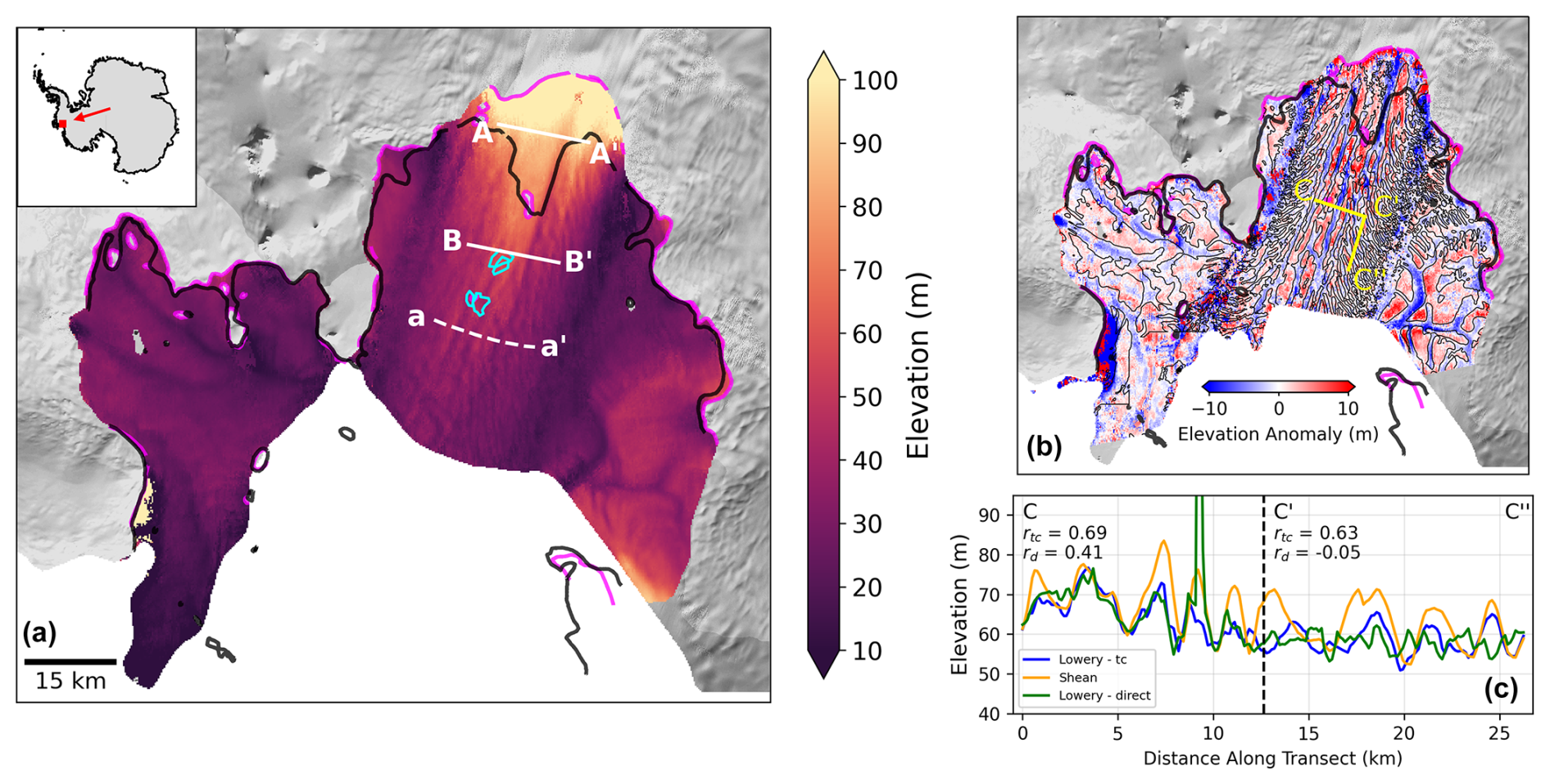
Figure 1 (a) A digital elevation model (DEM) of Pine Island Glacier from July 2017, derived from CryoSat-2. The white transects correspond to sections used in Fig. 7. The cyan contours in (a) show areas of ephemeral regrounding in 2017, as observed from Sentinel-1 using the differential range offset tracking method (described in Sect. 2.3). Panel (b) shows a high-pass filtered CryoSat-2 DEM from December 2012. It is overlaid with the 0 m contour line from a high-pass filtered Shean et al. (2019) DEM in black. The yellow transects are used in panel (c). Both (a) and (b) also have the 1996 and 2011 MEaSUREs grounding lines in black and magenta, respectively (Rignot et al., 2016). The background of (a) and (b) uses a greyscale Landsat Image Mosaic of Antarctica (LIMA) at 15 m resolution. Panel (c) shows elevation profiles from our time-centred DEMs, our DEMs using the direct method, and the Shean et al. (2019) DEM along the transect between C, C^′, and C^′′ in (b). The correlations of each of our methods with the Shean et al. (2019) DEM along the two sections of this transect are also shown.

2 Data and methods

2.1 CryoSat-2 surface elevation data

We generate DEMs using CryoSat-2 (CS2) SARIn swath-processed radar altimetry data (Gourmelen et al., 2018). Over the Pine Island embayment area shown in Fig. 1a, there are approximately 180 million elevation measurements between 2011 and 2023. These measurements are used to create monthly DEMs with a spatial resolution of 250 m. To achieve full coverage at this spatial resolution, each DEM requires a year's worth of data. We therefore produce a product with an annual resolution at monthly posting, as described below.

Before creating our DEMs, many corrections are first applied to the CS2 observed ice shelf surface elevation data. Each CS2 elevation measurement has been corrected for tides, the inverse barometer effect (IBE), and firn air content. Tidal corrections have been applied from the CATS model outputs (Howard et al., 2019), and IBE corrections have been taken from the CNES SSALTO system provided by Meteo France. Firn air content has been taken from the Institute for Marine and Atmospheric research Utrecht (IMAU) firn densification model forced by RACMO model outputs (Veldhuijsen et al., 2023). We also note that the swath processing relies on the presence of an across-track surface slope to prevent left–right phase ambiguities. This can be challenging over some ice shelves. However, many studies have shown that we can retrieve swath elevation measurements for a significant portion of CS2 waveforms over many ice shelves (Gourmelen et al., 2017; Davison et al., 2023; Surawy-Stepney et al., 2023; Wuite et al., 2019; Goldberg et al., 2019). It is thought that the slight mispointing of CS2 prevents the complete cancellation of returns and therefore contributes to the coherence of data in these regions (Recchia et al., 2017). Once the corrections have been applied, any data of low quality have been removed. If the return has a coherence of less than 0.6 or its absolute difference with the Reference Elevation Model of Antarctica (REMA) is greater than 100 m, then the data have been removed.

The 12 months of data that are required to create a single DEM are centred around the target date that the DEM represents. The target date is the 1st of the month, and all elevation data within 6 months of this date are gathered and advected to the location at which they would have been on the target date using ice velocity data. For example, if we were creating a DEM on 1 July, all observations acquired between 1 January and 30 June of the same year would be advected forward to their location on 1 July, and all observations between 2 July and 31 December would be advected back to their location on 1 July. This process will be referred to as “time-centring” from here onwards. Specifically, if a given elevation measurement, h, is recorded in month m₀ with a location of (x₀, y₀) and the DEM being created is centred on month m_n, its time-centred location is given by:

$$\begin{array}{}\text{(1)}& (x_n,y_n)=\left(x_{\mathrm{0}}+\sum _{i=\mathrm{0}}^{n-\mathrm{1}}{u}_i\mathrm{d}t,y_{\mathrm{0}}+\sum _{i=\mathrm{0}}^{n-\mathrm{1}}{v}_i\mathrm{d}t\right),\end{array}$$

where u_i and v_i are the velocities in the x and y directions, respectively, evaluated at the (x, y) location of h at time step i and dt is the time step duration. Once this advection procedure has been applied to all measurements within 6 months of the target date, the resultant data points are gridded into 250 m × 250 m bins, and that bin takes the median value of all its members. Advection is calculated using the ITS_LIVE annual velocity mosaics (Fig. 2b) with a monthly time step. With CS2 surface elevation data spanning from January 2011 to December 2023, our monthly DEMs start from July 2011 and extend to July 2023.

We have chosen to implement this time-centring method because it more accurately represents the surface of the ice shelf when combining a year of data than by directly binning the observations (Figs. 1c and A1). Temporal averaging is required to obtain 250 m horizontal resolution but, over a year of coverage, a parcel of ice could have crossed 16 of the 250 m grid boxes (assuming a velocity of 4 km yr⁻¹). By simply binning these observations, ice shelf surface geometries will be smoothed over a few kilometres, removing our ability to observe changes within channels and any features that are not exactly aligned with ice flow. By adopting the time-centring process, we reduce the aliasing of these features (Fig. 1c). Along the main trunk of the ice shelf, the distribution of surface troughs and ridges (associated with basal channels and keels) in our time-centred DEMs shows a good agreement with a higher-resolution but less frequently acquired, WorldView-derived DEM from Shean et al. (2019) (Fig. 1b). While our CryoSat-2 DEMs successfully capture the primary longitudinal channel features, they do not resolve small transverse channels as clearly. However, the time-centring method captures these surface features with substantially greater accuracy than the direct method (Fig. 1c). Between C^′ and C^′′ of the transect shown in Fig. 1b, the correlation with the Shean et al. (2019) DEM improves from −0.05 using the direct method to 0.63 with the time-centring approach.

Despite the overall consistency in feature distribution, our CryoSat-2 DEMs underestimate the amplitude of channels relative to the Shean et al. (2019) product (Fig. 1c). This underestimation occurs primarily because of an underestimation of the surface ridges. While there are a number of reasons for this bias (firn penetration, averaging in time, etc.), we assume that it is consistent in time and therefore does not impact the temporal change observed throughout this paper.

The DEMs are generated by advecting elevation data to their estimated positions on the target date, while neglecting changes in ice thickness during this process. Although this assumption introduces some uncertainty, its impact on the final DEM is minimised because the advection is performed both forward and backward in time. Specifically, a measurement advected forward by six months (and therefore experiencing six months less melt) is balanced by a measurement advected backward by six months (experiencing six months more melt). By taking the median value within each bin, these opposing effects largely cancel each other out, resulting in a robust representation of elevation (Fig. 1b and c).

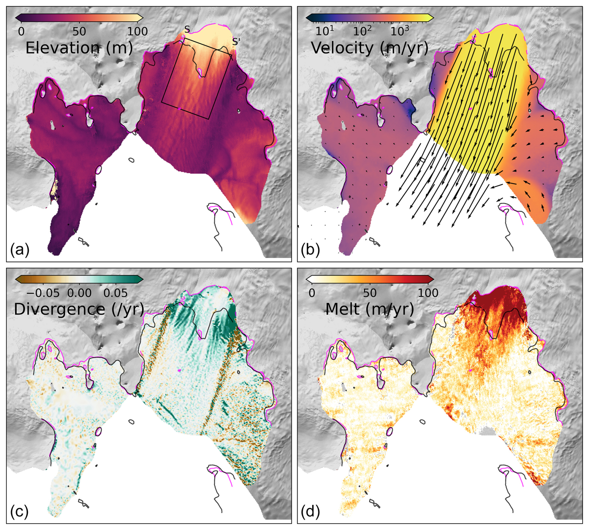
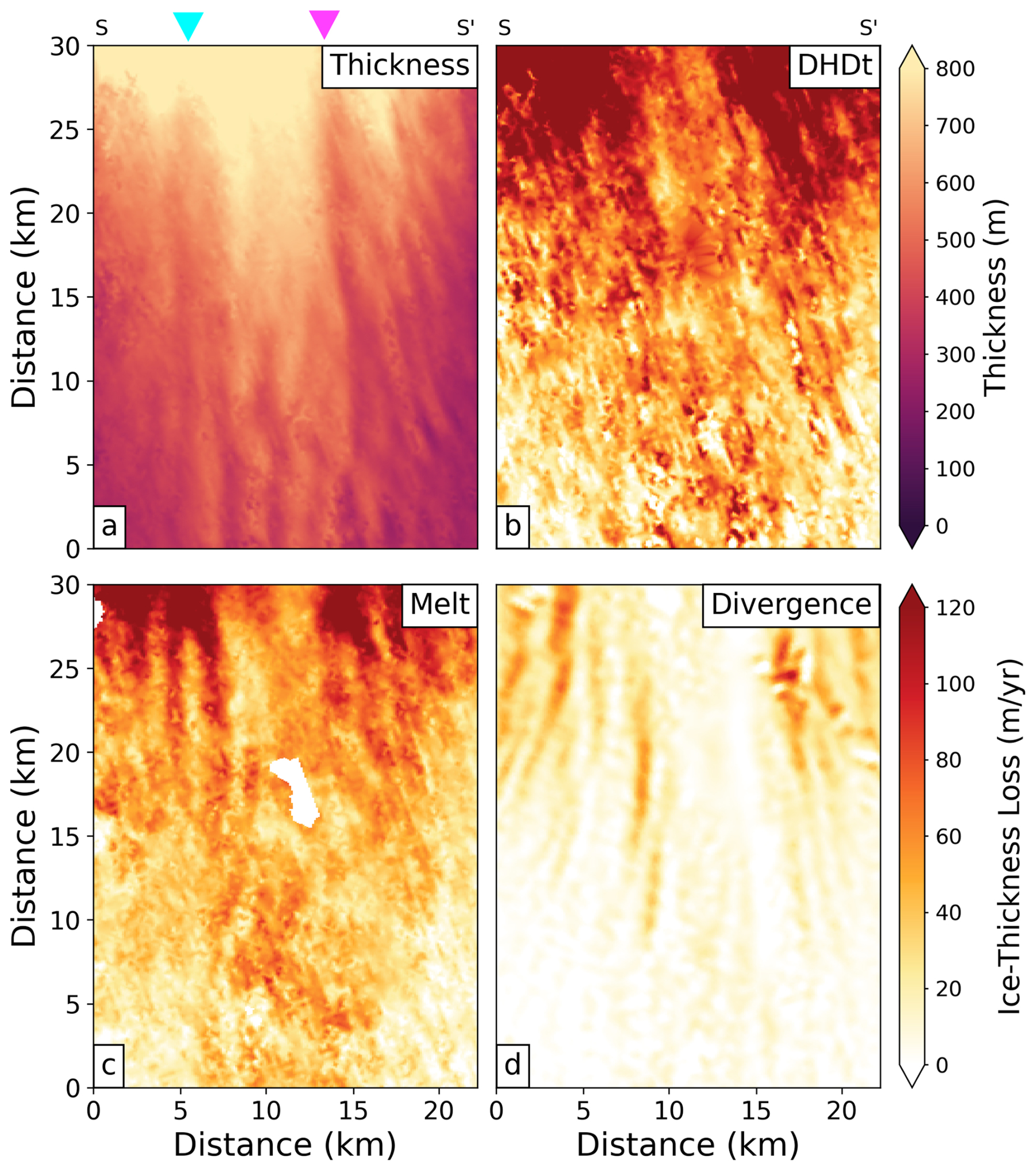
Figure 2 (a) A digital elevation model derived from CryoSat-2, (b) velocity, coloured by velocity magnitude and overlaid with velocity vectors, (c) velocity divergence, and (d) basal melt rates. All components shown are from 2015. The black rectangle in (a) corresponds to Figs. 5 and 6. The basemap and grounding lines are the same as those in Fig. 1.

2.2 Basal melt calculations

Once monthly DEMs are generated, we use them (e.g. Fig. 2a) to calculate Lagrangian basal melt rates (Fig. 2d) by employing a similar method to those detailed previously (Shean et al., 2019; Dutrieux et al., 2013; Zinck et al., 2023; Moholdt et al., 2014; Gourmelen et al., 2017). The Lagrangian framework measures the thickness change of a parcel of ice as it moves, thereby avoiding issues associated with the advection of topographic features through the grid that arise within an Eulerian framework. Assuming floatation of the ice, basal melt rates, m, are given by:

$$\begin{array}{}\text{(2)}& m=-{\displaystyle \frac{\mathrm{D}H}{\mathrm{D}t}}-H(\mathrm{\nabla }\cdot \mathit{u})+s,\end{array}$$

where

$$\begin{array}{}\text{(3)}& H=h\left({\displaystyle \frac{{\mathit{\rho }}_{\mathrm{w}}}{{\mathit{\rho }}_{\mathrm{w}}-{\mathit{\rho }}_{\mathrm{i}}}}\right)\end{array}$$

is the ice thickness, $\frac{\mathrm{D}H}{\mathrm{D}t}$ is the Lagrangian thickness change, u is the horizontal ice velocity vector, H(∇⋅u) is the thickness change resulting from flow divergence, and s is the surface mass balance (SMB), positive for accumulation. SMB has been taken from RACMO model outputs (Noël et al., 2018). By assuming hydrostatic equilibrium and constant ocean and ice densities, ρ_w=1028 kg m⁻³ and ρ_i=917 kg m⁻³, respectively, ice elevation, h, is converted into ice thickness, H, following Eq. (3). Within the ice flux divergence term, H(∇⋅u), of Eq. 2, H is taken from the initial DEM.

For each month, we conduct the same advection process as described in Sect. 2.1 to predict the location of an ice parcel after a year. Subsequently, the Lagrangian thickness change is determined by comparing the ice thickness at the original location with the thickness at its location a year later. This process yields a Lagrangian change in thickness $\left(\frac{\mathrm{D}H}{\mathrm{D}t}\right)$ map that is temporally centred between the two DEMs, at the “mid-time” stamp half a year after the start date. The Lagrangian thickness change is allocated to its original location in space, following the “initial pixel” method outlined by Shean et al. (2019). The change in ice thickness as a result of velocity divergence (H(∇⋅u), Fig. 2c) is considered based on the original location of the ice parcel at the mid-time stamp and is again calculated using the annual ITS_LIVE velocity mosaics (Fig. 2b).

Throughout the method, we use an annual velocity dataset. Over our observational period, PIG accelerates and the flow bends westward (Fig. A2) following the large calving events in 2018. Therefore, using a time averaged velocity field would not be appropriate. However, using annual velocity datasets introduces discrete jumps at annual boundaries. Furthermore, the annual velocity datasets are relatively noisy, and this likely contributes to some noise in our melt maps. During the advection process (both for time-centring and melt advection), the velocity dataset corresponding to the year of each time step is used. Similarly, the divergence field for the melt calculation is taken from the year of the target month. We decided against interpolating between velocity datasets to avoid smoothing the channel-scale features we aim to preserve within the velocity and divergence fields (Fig. 6d). The aliasing of channel-scale features when interpolating between these fields would become more prominent when channels are not aligned along flow. Our choice ensures consistency throughout the method by aligning the treatment of velocity and divergence fields.

The velocity divergence, ∇⋅u, is calculated over a 480 m (two times the resolution of the velocity dataset) length scale using a centred calculation. For a given grid cell, divergence is calculated from the velocity gradient between its neighbouring cells. The output is therefore spatially centred on the initial grid cell of interest. This scale is relatively small with respect to the channel width, so we expect to capture the channelised signal of divergence without smoothing the signal within a channel. However, it is likely that signals at the channel edge are somewhat smoothed as the calculation computes gradients between points on either side of the channel boundary.

At the channel scale, our monthly posted melt maps remain relatively noisy. To further reduce the noise and obtain a coherent channelised melt signal, we further averaged 12 months of melt maps. To complete this averaging, we have advected the 12 months of melt data to their location at the middle time step using the same advection process as during time-centring, as described in Sect. 2.1. The advected data are then rebinned, and the median melt value in the bin is taken. This averaging has been completed on a rolling 12 month basis, and therefore we retain monthly posting between July 2012 and December 2021. Between the time-centring associated with the creation of the DEMs and that associated with noise reduction of the melt maps, elevation data spanning 3 years have contributed to each monthly posted melt map.

The averaging of annual melt maps was completed within a Lagrangian framework to avoid smoothing channelised melt anomalies that are not aligned with flow. While ocean conditions set the amount of heat in the cavity, the melting that occurs depends on the ability of ocean circulation to bring the heat to the ice–ocean interface. These currents depend on ice shelf geometry on both large scales and channel scales. Therefore, ice movement changes the spatial distribution of melt, and Eulerian averaging would smooth over these changes.

Obtaining basal melt rates with this approach is based on several key assumptions. Specifically, it assumes that the ice is fully floating and in hydrostatic equilibrium, that the ice velocity is vertically uniform (and therefore the surface velocity is a good representation of the ice velocity at the base), and that the ice is a viscous continuum (i.e. does not fracture in response to divergence) (Dutrieux et al., 2013; Zinck et al., 2023). Bridging stresses within the ice make deriving changes within small channels through changes in surface elevation challenging (Dutrieux et al., 2013). It is important to acknowledge these limitations inherent in methods using remote sensing techniques to derive ice shelf basal melt rates, particularly when attempting to infer changes to features of similar scales to a few ice thicknesses. Furthermore, in situ surveys have demonstrated the complexity of the basal geometry associated with smoother surface expressions (Dow et al., 2024; Dutrieux et al., 2014b; Drews, 2015). We also note that the RACMO SMB data have relatively low spatial resolution compared with the width of channels, leading to undersampling across the channels. Although some evidence suggests that SMB can vary asymmetrically across channels (Drews et al., 2020), this is unlikely to affect our results, as the basal melt signal is much larger than the SMB signal.

2.3 Sentinel-1 differential range offset tracking

To investigate the relationship between channels and pinning points, we derive the locations of pinning point groundings using the differential range offset tracking (DROT) method applied to Sentinel-1 synthetic aperture radar (SAR) data. The DROT technique makes use of SAR sensors' off-nadir viewing geometry to detect floating ice, because vertical tidal displacements are projected into the satellite's line-of-sight and appear as an anomalous horizontal ground range displacement in intensity feature tracking results (Joughin et al., 2016; Friedl et al., 2020; Marsh et al., 2013). By differencing adjacent feature tracking results or subtracting a reference steady-state ground range velocity field, the anomalous ground range displacement caused by vertical tidal displacement is isolated, in a process analogous to differential interferometric SAR (DInSAR). From this tidal displacement result, the grounding line and any pinning points can be delineated. Because DROT uses intensity feature tracking, rather than InSAR, to measure ice motion, it does not require InSAR coherence and is suitable for investigating pinning points on fast flowing ice shelves, such as PIG, where coherence is not routinely maintained in the 6 d repeat period of Sentinel-1.

In this study, we use 6 and 12 d repeat Sentinel-1 intensity feature tracking pairs over the PIG shelf processed using the GAMMA remote sensing software package (Strozzi et al., 2002). Tracking results are post-processed using a moving mean filter over a 1×1 km window, where values 30 % greater than the mean are rejected and isolated pixels that represent poor tracking results are also removed according to a locally determined threshold (Lemos et al., 2018; Selley et al., 2021). Outputs are posted at a resolution of 100×100 m in Antarctic Polar Stereographic projection (EPSG:3031). To produce observations of ephemeral grounding and pinning points, we select acquisition pairs with differential tide heights greater than 0.5 m and remove the steady-state ground range velocity field by subtracting the median ground range velocity from a 180 d window centred on the measurement date to calculate the tidal motion anomaly. This anomaly is manually delineated with GIS software to determine the location of any grounded portion of the ice shelf for the selected acquisition pair.

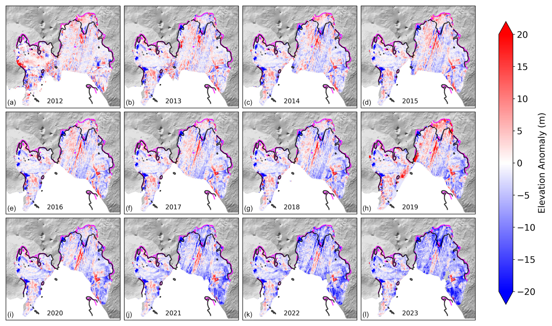
Figure 3 (a)–(l) show the annual elevation anomalies with respect to the first DEM in June 2011 for 2012–2023. Basemap and grounding lines are the same as those in Fig. 1.

3 Results

3.1 Channel and pinning point history

Over the 2011–2023 observed period, the PIG calving front retreated (Joughin et al., 2021) and the ice shelf thinned by an average of 60 m, equivalent to a mass loss of 259 Gt through thinning alone (Fig. 3). In addition to overall thinning, geometric features such as basal channels have evolved, imprinting small-scale features on the overall thinning pattern (Fig. 3).

A pinning point in the centre of the ice shelf began to unground in 2011 (Joughin et al., 2016), resulting in a thick column of ice being advected downstream. This is visible in the anomalously thick (red) region in the centre of Fig. 3a. Over time, the entire downstream section of the ice shelf thickened as the thicker ice was transported further downstream (Fig. 3). The thick ice ephemerally regrounded as it advected downstream (Joughin et al., 2016).

In 2011, a large basal channel extended downstream of the pinning point, as shown in Fig. 4a (beyond 8 km) and in the centre of Fig. 4d. We hypothesise that this channel formed due to interactions between the ice and bed at the pinning point, which imprinted on the ice geometry, and was further enhanced by concentrated melting within the channel. After the pinning point ungrounded, this basal channel was gradually advected downstream and replaced by thicker ice. Therefore, the thickening trend shown in Fig. 3 is as much a signal of the absence of a channel as of thickening with respect to the whole ice shelf. Simultaneously, a new arrangement of basal channels began forming further upstream (Figs. 3 and 4).

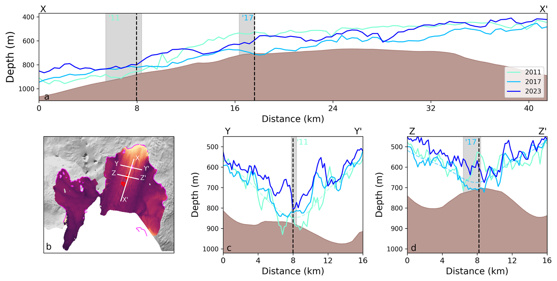
Figure 4 Depth of the ice shelf base in 2011, 2017, and 2021 across three different transects. (b) shows the three transects used in the other subplots. (a) shows the depth of the base between X and X^′, (c) shows the depth of the base between Y and Y^′, and (d) shows the depth of the base between Z and Z^′. The red lines in (b) show the areas where Sentinel-1 DROT data indicate grounded ice in 2017. The vertical grey shaded areas in (a), (c), and (d) show grounded areas in 2011 and 2017, as observed by the MEaSUREs 2011 grounding line and DROT 2017. The black dashed vertical lines mark the points of intersection between transects. The brown shaded areas on (a), (c), and (d) are the seabed from BedMachine, merged with observations from Dutrieux et al. (2014b).

To investigate the relationship between basal channel distribution and grounding, we will focus on the change in the ice base depth over our observational period across three transects (Fig. 4). The depth of the ice shelf base has been calculated by inverting the surface elevation and assuming floatation:

$$\begin{array}{}\text{(4)}& d=-h\left({\displaystyle \frac{{\mathit{\rho }}_{\mathrm{i}}}{{\mathit{\rho }}_{\mathrm{w}}-{\mathit{\rho }}_{\mathrm{i}}}}\right).\end{array}$$

Across all three transects, the depth of the ice shelf in 2011 (cyan), 2017 (blue), and 2023 (dark blue) has been plotted. These years represent when the pinning point was starting to unground (2011), when the pinning point ephemerally regrounded in the centre of the ice shelf (2017), and the end of our observation period (2023), when the DROT method detects no further grounding, and the long-term impact of the unpinning on the distribution of basal channels can be assessed. The transect in Fig. 4a is along flow (shown between X and X^′ in Fig. 4b) and intersects areas where the pinning point was observed to be grounded in both 2011 and 2017. The transect in Fig. 4c is across flow (shown between Y and Y^′ in Fig. 4b) and intersects where the pinning point was grounded until 2011. The third transect in Fig. 4d is shown between Z and Z^′ in Fig. 4b and intersects the location where Sentinel-1 observes the ice shelf to be ephemerally grounded in 2017. All three of these plots also show the depth of the seabed from BedMachine after merging with data collected from Dutrieux et al. (2014b) along their respective transects. Grey, vertically shaded areas show areas along the transects where the ice was grounded according to MEaSUREs grounding lines in 2011 and Sentinel-1 in 2017. Dashed lines are also plotted in Fig. 4c and d. These correspond to the depth of the smoothed ice base in 2011 and 2017, respectively.

Despite the overall ice shelf thinning during this period (Fig. 3), the ice base depth along the along-flow transect does not exhibit a straightforward, uniform thinning rate (Fig. 4a). Downstream of the 2011 pinning point location (the shaded grey region, approximately 6–8 km along the transect), the ice shelf base is shallowest in 2011 and deepest in 2017. The 2011 depth represents the apex of the downstream channel discussed earlier (and is also visible in the 2011 base depth shown in Fig. 4d). By 2017, this section of the ice shelf had thickened significantly as the thick column of ice was advected downstream, filling in the basal channel. By 2023, however, the entire ice shelf had thinned, and no part of this transect remained in contact with the seabed. The two across-flow transects (Fig. 4c and d) reveal a more predictable relationship between time and thinning. Overall, the ice shelf base becomes progressively shallower over the observational period, with the exception of the basal channel visible in the 2011 ice shelf base, as shown in Fig. 4d. The contrast between this channel in the centre of the transect in 2011 and the grounding of the ice in 2017 illustrates how the thick column of ice was advected downstream from the initial pinning point location and changed the geometry of the ice shelf.

Figures 4c and d also demonstrate how basal channels contributed to the persistence of the pinning point and the intermittent regrounding of the subsequent thick ice column. In both figures, a hypothetical smoothed version of the ice shelf base is shown. This ice base represents what we might expect if channels and channelised melt did not exist and hence if all ice shelf melt were uniformly distributed across the ice shelf. In both instances, the ice shelf would not have regrounded, instead it would have left a 30 m deep cavity between the ice shelf base and the seabed. This suggests that without a pronounced channel and keel geometry on the ice shelf base, the pinning point might not have been sustained for as long, and the thick ice may not have periodically regrounded.

Unsurprisingly, some discrepancies exist between the grounded area predicted by Sentinel-1 DROT methods and the locations inferred by comparing CS2 ice base data with the modified BedMachine seabed depth data. Several factors contribute to this difference. The base depth calculated by inverting the elevation is derived by assuming that the ice shelf is in hydrostatic equilibrium, which we know does not hold near grounded regions. Further, the CS2 DEMs – and consequently the ice draft – are calculated by averaging data points over a full year, which may smooth some of the finer details. Channelised structures are also under-represented on the ice surface due to bridging stresses (Wearing et al., 2021; Drews, 2015) and kilometre-scale gradients in ice density (Dutrieux et al., 2013), potentially driven by surface meltwater pooling in channels that increase the firn density (Drews et al., 2016). Hence, our derived ice shelf base depth may not capture the full channel geometry. Despite these limitations, our observations align reasonably well with those from Sentinel-1.

Figure 5 Thickness (a), Lagrangian thickness changes (b), basal melt (c), and ice flux divergence (d) in the black rectangle in Fig. 2a. All variables are from 2015.

3.2 Channelised melt

We next use these data to assess the spatial distribution of ice shelf melt at a channel scale. To do this, we focus on the area shown by the black rectangle in Fig. 2a. Figure 5 shows the thickness, Lagrangian thickness change, melt centred in July 2015, and ice flux divergence in 2015. Basal melt is the largest contributor to ice thickness loss here (>100 m yr⁻¹ compared with ∼40 m yr⁻¹ from ice flux divergence).

In the area shown, basal channels are clearly present within the thickness map (Fig. 5a, marked by the cyan and magenta arrows). However, they cannot be seen in the thickness change variables (Fig. 5b–d). This is not necessarily surprising; it simply suggests that in this location the change in Lagrangian thickness and flux divergence is similar inside and outside of channel. To investigate the channelised pattern of ice loss, we will now focus on the high-pass filtered anomalies of these fields (Fig. 6), which have been calculated by subtracting a 2-D Gaussian low-pass filter with a radius of 7 km, similar to Dutrieux et al. (2013) and Shean et al. (2019). In Fig. 6, a positive ice loss anomaly means more thinning, and a negative ice loss anomaly shows less thinning. Therefore, if the focus is on a channel, a negative anomaly indicates that the channel amplitude is decreasing and a positive anomaly indicates that the channel amplitude is increasing.

There are two main channels within this area, which can be seen from the negative (blue) thickness anomaly in Fig. 6a. They both extend the entire length of the area with little across-flow deviation. The channel indicated by the magenta arrow will be referred to as Channel 1, and the channel indicated by the cyan arrow will be referred to as Channel 2 from now on. Both Channels 1 and 2 are approximately 2 km in width, but Channel 1 has an amplitude of 160 m, whereas Channel 2 has an amplitude of only 80 m. Channelised melting can be detected in both of these channels near the grounding line and particularly on the channels' western flanks, where anomalies exceed 30 m yr⁻¹. The channelised melt pattern becomes less prominent downstream. There is also a group of smaller channels on the southern side (bottom right) of this area, which are more variable in distribution, but our method does not detect a channelised melt distribution within these smaller channels.

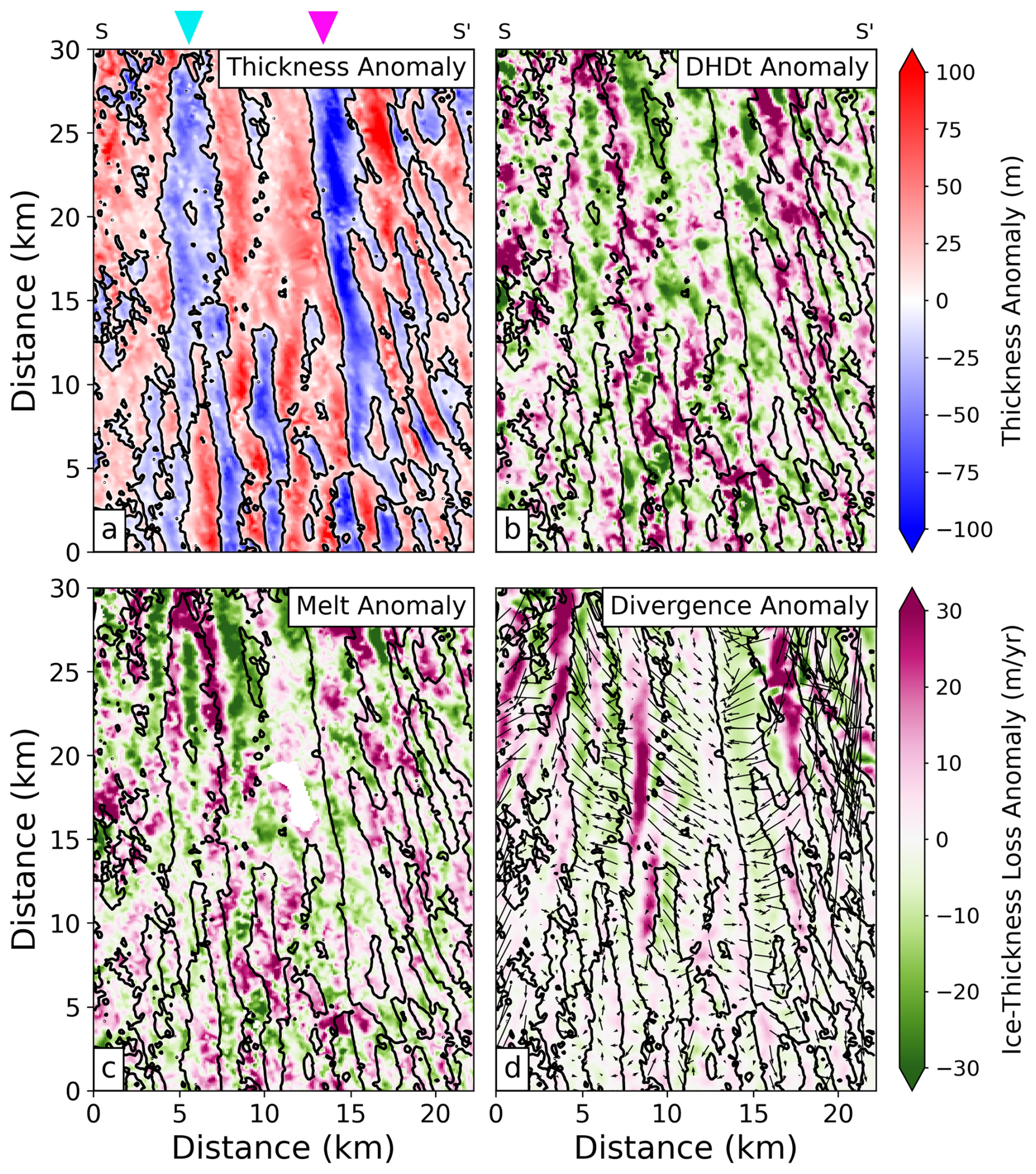
Figure 6 High-pass filtered anomaly of thickness (a), Lagrangian thickness change (b), basal melt (c), and ice flux divergence and velocity (d) within the black rectangle in Fig. 2a. All variables are from 2015. The pink and cyan arrows indicate Channels 1 and 2, respectively, as discussed in the text.

Figure 6d displays the ice flux divergence anomaly overlaid with velocity anomaly vectors, illustrating the influence of basal channels on both ice flux divergence and velocity. Ice flow converges into basal channels and diverges away from basal keels. This pattern can be seen right down to the smaller channels on the southern side of the area, where channels are just 1 km wide with amplitudes of less than 50 m. This channel-scale distribution of secondary ice flow is consistent with a viscous response to ice thickness gradients (Wearing et al., 2021).

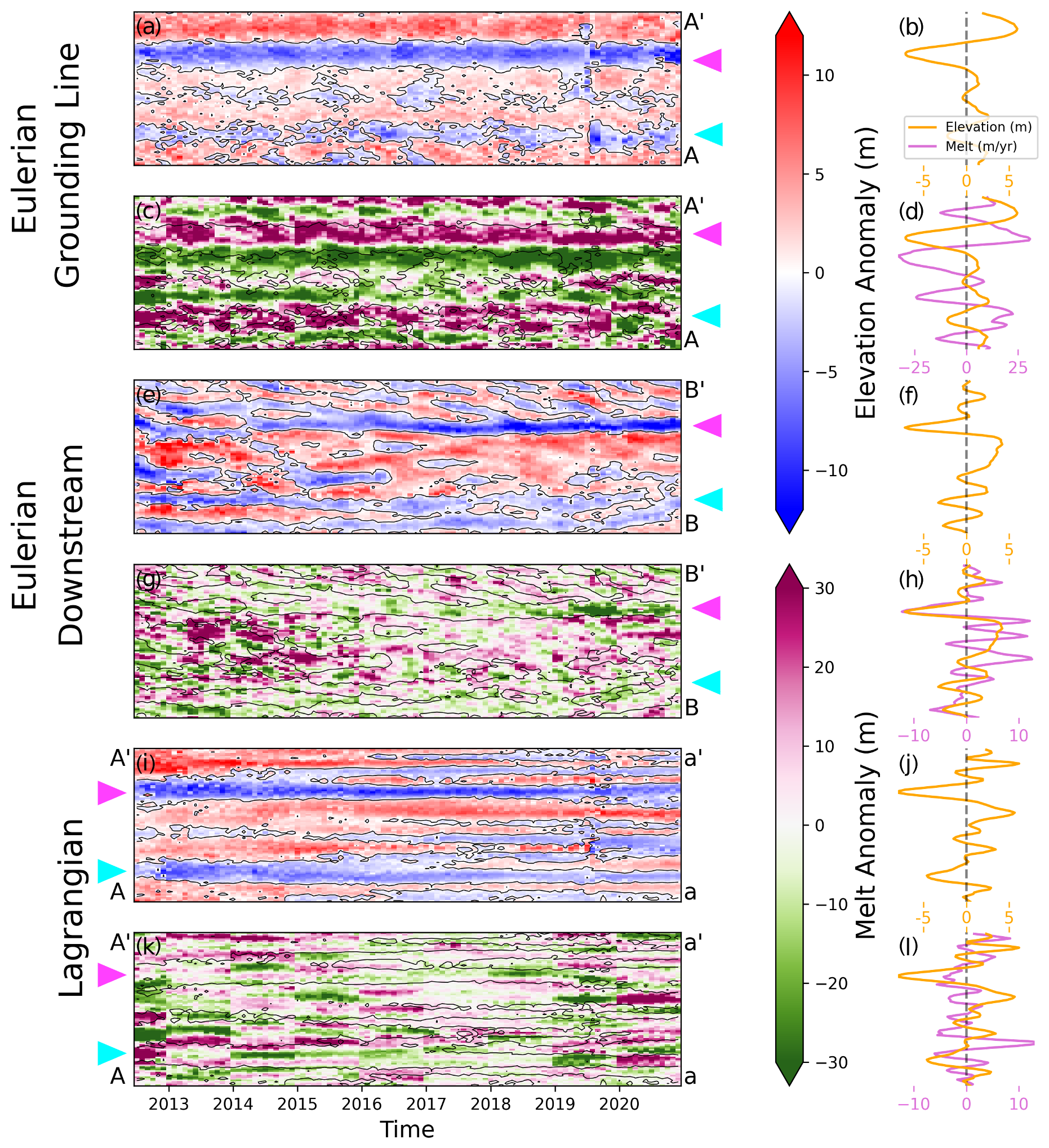
Figure 7 Elevation and melt anomaly evolution for different sections on the ice shelf. (a) and (c) are the elevation and melt anomalies between A and A^′ in Fig. 1. (e) and (f) are the elevation and melt anomalies between B and B^′ in Fig. 1. (i) and (k) are the elevation and melt anomalies originating from A and A^′ in Fig. 1 in a Lagrangian framework. This transect has been advected forward in time until it is between a and a^′ at the end of 2020. (c), (g), and (k) are overlaid with the zero contour line from (a), (e), and (i), respectively, in black. The right-hand column of panels shows the time averaged value of elevation and melt from the adjacent panel. The pink and cyan arrows indicate Channels 1 and 2, respectively, as discussed in the text.

3.3 Channelised melt evolution

Although previous studies have used DEMs with a higher spatial resolution to derive melt rates (Shean et al., 2019; Zinck et al., 2023), these are less frequently acquired. The strength of CS2 data resides in their long-term stability and the frequency of their sampling. With an annual moving window averaging technique, we can observe how channelised features evolve at sub-annual timescales. Figure 7 shows the elevation (panels a, e, and i) and melt (panels c, g, and k) anomalies along different sections of the ice shelf during our observing period. As in Fig. 6, small-scale high-pass filtered anomalies are taken with respect to a Gaussian 2D filter with a radius of 7 km. The Gaussian filter and, therefore, the high-pass anomalies are recalculated at every time step. The right-hand column of Fig. 7 shows the time averaged elevation (yellow in panels b, d, f, h, j, and l) and melt (pink in panels d, h, and l) anomalies across the different sections.

Figures 7b and d show the elevation and melt anomalies, respectively, across a transect near the grounding line (solid white transect between A and A^′ in Fig. 1a), where the ice shelf geometry has not been directly affected by the ungrounding of the pinning point. These panels show the transect in an Eulerian framework, so the transect location is static in time. During this period, Channels 1 and 2 have a consistent geometry (Fig. 7a) and are associated with positive melt anomalies of 30 and 20 m yr⁻¹, respectively, along their apexes (minima in surface elevation anomaly correspond to maxima in melt anomaly) (Fig. 7c and d).

Figures 7e and g present the elevation and melt anomalies, respectively, across a downstream transect (solid white line between B and B^′ in Fig. 1a). As in Fig. 7b and d, the transect is fixed in time in an Eulerian framework. The transect is about 10 km downstream of the 2011 pinning point location and, therefore, the elevation and melt rates across it are directly influenced by the changes in pinning point geometry. In contrast to the transect near the grounding line, the geometry here is rapidly evolving during the start of the observed period. However, following 2015, a persistent channel forms in the south of the transect, which corresponds to the upstream location of Channel 1. The stabilised geometry is likely a reflection of the pinning point ice advecting past the transect, and hence a seamless connection between the grounding line and the transect has opened. Within this channel, a sustained negative melt anomaly emerges after 2016. Despite the channel's consistent geometry only occurring in 2015, the time averaged melt anomaly in this area remains strongly negative (Fig. 7h).

This contrast in channel melt anomalies between those near the grounding line and those further downstream highlights a regime shift between the near grounding line, where channels are carved, and a few kilometres downstream, where the channel's amplitude decreases through greater melting of its keels. This is consistent with our understanding that plume dynamics have the greatest control on melt rates near the grounding line, but the depth-dependent freezing point and vertical ocean temperature distribution become more relevant downstream (Gladish et al., 2012; Dutrieux et al., 2013).

Figures 7i and k offer a Lagrangian perspective, tracking the evolution of the A–A^′ transect from Fig. 7a and c as it moves downstream on the ice shelf through to 2021. This method allows us to follow the transformation of a single cross section of ice over time. By late 2021, the transect had reached the dashed white line between points a and a^′ in Fig. 1a.

Initially spanning 2 km in width, Channel 1 persists throughout the observational period but undergoes geometric changes. Smaller channels, approximately 1–1.5 km wide, branch off the central feature. While the primary orientation of Channels 1 and 2 remain relatively stable, these smaller branches appear to veer westward, similar to the observations from Bindschadler et al. (2011). This process nearly doubles the channel wavenumber (the number of channels per unit distance) as the transect moves downstream (Fig. 7i).

The melt signal within the Lagrangian framework appears noisy and exhibits discontinuous steps at yearly boundaries (Fig. 7k), due to the changes in the divergence field used in the melt calculation. While smaller discontinuities are visible in the melt product of the two Eulerian transects, the combination of changing space and time in the Lagrangian framework emphasises the impact of these discrete steps in the divergence field.

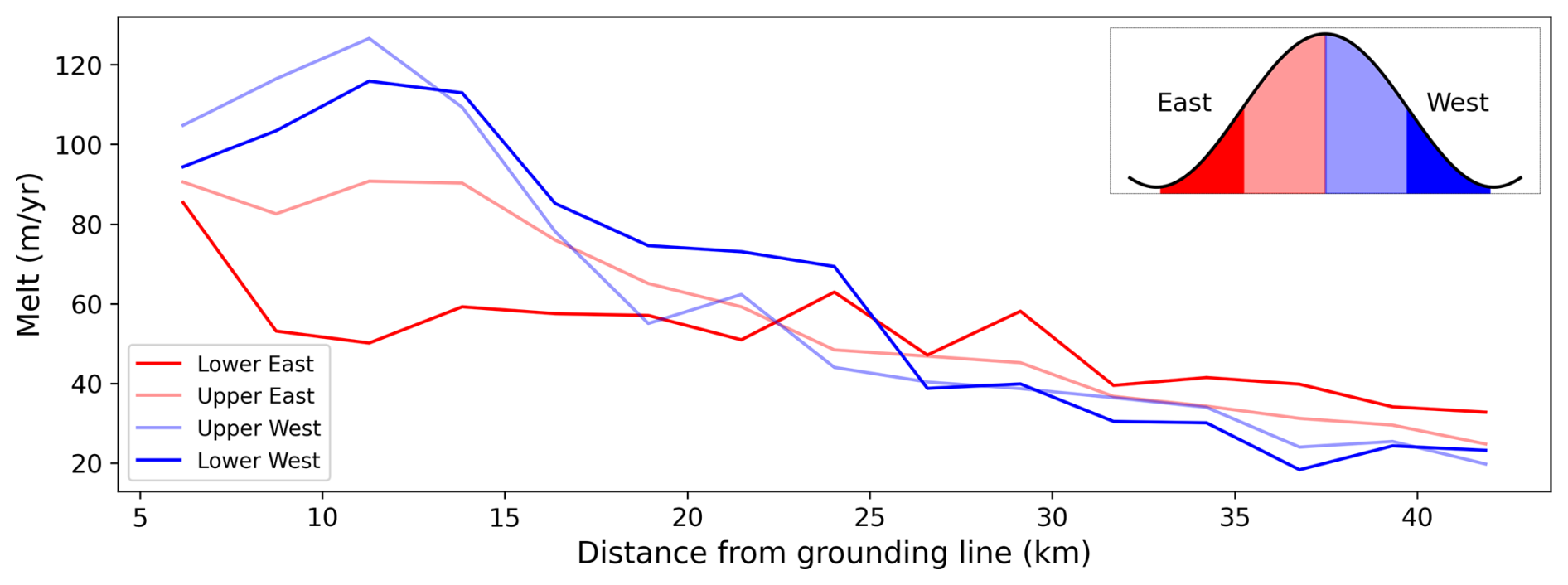
Figure 8 Comparison of melt rates along different sections of Channel 1 as a function of distance from the 2011 grounding line.

3.4 Coriolis-favoured melting

Several studies have hypothesised and sporadically observed that melting in channels is enhanced on the Coriolis-favoured side, particularly near the grounding line (Gladish et al., 2012; Millgate et al., 2013; Dutrieux et al., 2013; Gourmelen et al., 2017; Marsh et al., 2016; Cheng et al., 2024). To further investigate the asymmetric distribution of melting across a channel (Fig. 7c and d) and how this distribution varies as a function of distance from the grounding line, we now consider Channel 1 in more detail. This channel has been chosen because it is persistent in time and by the end of the observing period it extends to the calving front (Fig. 7e), and we also derive the largest melt signal within it. Therefore, we have the best chance of observing melt variations across it.

To investigate the across-channel variations in melt rates, we take across-channel transects ∼ every 2 km in the along flow direction, starting 6 km from the 2011 grounding line. Across each transverse transect, the channel apex and keels on either side are identified as the minimum and maximum small-scale elevation anomalies on either side, respectively. The eastern and western flanks thereby identified are further split into two equidistant subsections, effectively dividing the entire transect into four subsections from the eastern flank to the western flank of the channel (inset in Fig. 8). The boundaries of these subsections are recalculated for each transect every month. Melt rates calculated every month in each subsection are then averaged in time, providing us with a time averaged view of the melt distribution across the persistent Channel 1, from the grounding zone to the calving front.

The algorithm contains some criteria that the data must meet to be included in our analysis. Firstly, the depth of the channel apex must be shallower than that of the keels. Secondly, the identified channel must be at least 1.5 km in width (three grid points on either flank for a symmetric channel), and the length of each of its flanks must be within 1 km of each other. These criteria first ensure that the algorithm has correctly identified a channel and that there is no significant difference between the number of observations on either channel flank. This means that the selected channels are symmetric enough that a comparison can be made between the two flanks. Close to the grounding line, there are over 400 melt observations within each of the four subsections of the channel, whereas downstream there are ∼100 observations.

Near the grounding line, melt is highest on the upper western flank followed by the lower western flank (Fig. 8). Averaged between the eastern and western flanks, the melt on the western flank is over 50 % (40–50 m yr⁻¹) higher than on the eastern flank within the first 15 km of the grounding line. This asymmetry is likely driven by the Coriolis force acting on an ocean plume within the channel, which favours the erosion of the western keel (Fig. 9). Higher melting on the upper half of either flank also provides evidence that the melt distribution across the channel here is dominated by a buoyant plume within the channel. At 25 km or about half-way downstream from the grounding zone, the pattern reverses and melt rates on the lower eastern keel are highest (having dropped by only 40 % from the near grounding zone amplitude).

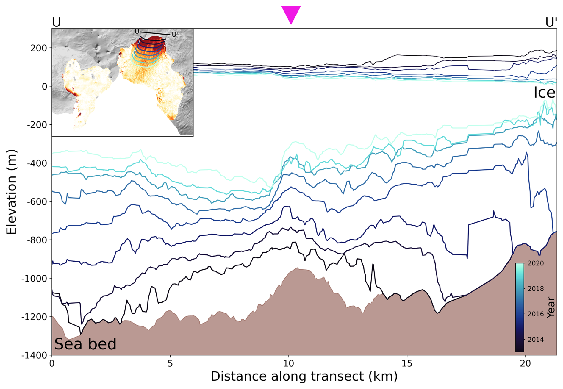
Figure 9 The brown area is the ice bed upstream of the grounding line along the black transect on the inset map, as measured from airborne radar (Vaughan et al., 2012). Using ITS_LIVE annual velocity data, the location of this flight line has been advected downstream, with the annual location of these advected transects shown on the inset map. The surface elevation and ice base depth derived from CryoSat-2 along each of these transects have then been plotted.

3.5 Channel formation

To predict how channel geometry – and consequently channelised melting – might evolve in the future, it is essential to understand how channels form. While various mechanisms of channel formation across Antarctica have been suggested by observations and modelled numerically (Le Brocq et al., 2013; Gourmelen et al., 2017; Marsh et al., 2016; Alley et al., 2016; Sergienko, 2013; Gladish et al., 2012; Millgate et al., 2013), the formation process on PIG remains uncertain. The persistence of Channel 1 throughout the CS2 observational period (Fig. 7a) provides new insights. This observation suggests a constant mechanism of formation that is closely linked to the grounding zone.

Figure 9 shows the seabed depth (brown) upstream of the grounding line (between U and U^′ on the inset map), as measured by airborne radar during the British Antarctic Survey campaign in 2004/05 (Vaughan et al., 2012). Starting in 2011, we advect the location of this flight line downstream with an annual time step. The surface elevation and depth of the ice shelf base as inferred from floatation along the advected flight lines are then plotted. We have only included transects where we are confident that the ice at Channel 1 is in hydrostatic equilibrium (greater than 2 ice shelf thicknesses away from the grounding line); hence, the first year shown is 2013.

In the centre of the grounded flight line, there is a ∼200 m high feature on the seabed surrounded by smaller (∼50 m high) oscillations. We note that a major part of the ice base evolution is connected to divergence from the shear margins and the associated thinning there, creating a convex glacier tongue with a thicker central line. The channelised geometry overlays and co-evolves with these large-scale changes. Channel 1 in the centre of the ice shelf appears to inherit its shape from the large central feature in the seabed. The channel begins symmetrically (as a reflection of the relatively symmetric bed feature) and gradually evolves to a more cliff-like topography in 2020 as a result of Coriolis-favoured melting, as discussed above (Sect. 3.4 and Fig. 8). These results suggest that channel geometry is in part a function of upstream seabed geometry on PIG and explain the persistent nature of Channel 1's geometry near the grounding line.

4 Discussion

Various approaches have been employed to calculate ice shelf melting using satellite observations (Dutrieux et al., 2013; Gourmelen et al., 2017; Zinck et al., 2023; Shean et al., 2019). In this study, we present the first time series of basal melt rates at a sub-kilometre spatial resolution, revealing the time-dependent nature of channelised geometries. On the PIG ice shelf, channelised geometries exhibit variability on annual timescales (Fig. 3), and both ice velocity and velocity divergence vary on spatial length scales consistent with channel structures (Fig. 6d). Relying on a time averaged dataset risks aliasing these dynamic features, potentially overlooking spatial variations in melt that contribute to the ice shelf integrated melt rate. Although this impact is especially pronounced on PIG, where abundant basal channels, rapid flow, and recent acceleration and redirection of ice flow (Fig. A2) complicate the dynamics, we expect similar considerations to be relevant across other ice shelves. Further investigation is needed to understand the implications of these methodological choices and to determine how they vary among different ice shelves. Ultimately, the method we propose may help refine historical mass loss estimates through better estimating the spatio-temporal variations of melting on sub-kilometre scales.

Furthermore, this methodological sensitivity may affect comparisons between satellite-derived melt rates and in situ observations. Precise consideration of the spatial context of in situ measurements relative to ice shelf geometry is essential. If satellite-derived melt rates alias spatio-temporal features, a meaningful comparison with in situ data becomes challenging.

We acknowledge several sources of error in both our methodology and data analysis. Noise in the CryoSat-2 data exists due to its poorly constrained firn penetration depth, from errors inherent in the unwrapping processes, and from orbit, range, and angle uncertainties. The median standard deviation in a single DEM bin is 5.8 m. There are also errors within the velocity product used. Although we have not completed a formal error propagation here, we believe these uncertainties do not alter our conclusions as they are likely consistent in time. However, a full investigation into how the different datasets used impact ice shelf basal melt rate estimation would be of benefit to the community.

Further errors arise from methodological assumptions. Most prominently, the method assumes that the ice shelf is in hydrostatic equilibrium. We know that this does not hold near the grounding line of an ice shelf. Throughout the analysis, we have used a conservative 2011 grounding line to mask the grounded ice. All basal channel analyses supporting our conclusions have been completed in areas of the ice shelf further than 2 ice thicknesses from the 2011 grounding line and therefore in an area of the ice shelf we consider to be, on the large scale, fully floating. However, hydrostatic errors also exist on a basal channel scale. Observations have shown that the depth of the ice base can be underestimated within basal channels (Dutrieux et al., 2013; Rignot et al., 2025) due to bridging stresses within the ice. It has also been shown that the largest errors in deriving melt rates from remote sensing data occur along channel walls, where bridging stresses across ice thickness gradients cause the ice shelf to deviate from hydrostatic equilibrium (Drews, 2015; Wearing et al., 2021). It is expected that melt is underestimated at the channel apex as a result (Wearing et al., 2021). This error is reduced as the ice relaxes while it moves away from the grounding line. This signal of relaxation is therefore aliased within our melt observations. While such errors may affect the quantitative melt rates derived, we do not expect them to influence our qualitative conclusions – for example, regarding Coriolis-favoured melting – as the errors should at least initially be symmetric across the channel.

The method we have used to estimate basal melt rates at a given timestamp (Sect. 2) uses elevation data spanning 3 years. All steps of the method use flow-line advection to time-centre the data and account for spatio-temporal changes. This approach addresses errors induced by feature advection through each observing window but at the cost of introducing temporal smoothing. This creates an effective along-flow smoothing kernel of 3 years (12 km if the ice shelf is flowing at 4 km yr⁻¹) but introduces no smoothing across flow. The method therefore permits shorter wavelengths in the across-flow direction than in the along-flow direction. Despite the disregard of the directional dependence of elevation change, we argue that this decision is critical to obtain channelised signals in our dataset.

Our observations show that melt rates near the grounding line are concentrated within basal channels (Fig. 8). While these observations agree with many others (Dutrieux et al., 2013; Marsh et al., 2016; Stanton et al., 2013; Gourmelen et al., 2017; Humbert et al., 2022; Zinck et al., 2023), they also contrast with observations made on the PIG ice shelf by Shean et al. (2019). There are a number of reasons why we might see these differences in our observations. Firstly, Shean et al. (2019) only noted the highest melting on channel keels within 3–4 km of the grounding line, an area where the hydrostatic assumption begins to break down. Further, in their study, channels were defined as any areas where the surface elevation anomaly was $<-\mathrm{1}$ m (equivalent to a thickness anomaly of ∼9 m) and keels where the elevation anomaly was >1 m (thickness anomaly greater than ∼9 m). It is therefore likely that observations classified as a keel in Shean et al. (2019) are defined as channel flanks in this study and the discrepancy arises from different labelling choices. We also note that the algorithm used in Shean et al. (2019) identifies large portions of the grounding zone to be basal keels, which might also affect the results. Furthermore, their channelised melt conclusions were deduced from a single composite melt map that spanned 7 years. It is therefore likely that across-channel melt variations were smoothed, and hence no conclusions were drawn regarding Coriolis-favoured melting. Conversely, our conclusions derive from analysis over only two persistent and larger channels, and a broader, more systematic study bringing in more observations (and associated caveats about the representation of smaller-scale features) may provide a more nuanced picture.

Our findings lend strong support to theories positing that channelised melt is concentrated on the Coriolis-favoured flank, where rising buoyant plumes are deflected by Earth's rotation (Gladish et al., 2012; Millgate et al., 2013; Marsh et al., 2016; Gourmelen et al., 2017; Cheng et al., 2024). Within 15 km of the grounding line, we observe ocean-driven melting to be approximately 50 % higher on the western flank than on the eastern flank, with the highest melt rates on the upper portion of the western flank (Fig. 8). Higher melt rates are also evident on the upper portion of the eastern flank relative to its lower portion. Our results are consistent with other studies positing enhanced melting on the channel apex. Notably, this pattern reverses downstream, where the eastern keel exhibits the highest melt rates. This can be explained by the deeper eastern keel being exposed to warmer (deeper) waters and therefore at a lower pressure-dependent freezing point. Alternatively, midwater intrusions arising from the calving front and an associated enhanced circulation could focus melt on this flank instead.

Consistent with previous observations (Alley et al., 2024) and modelling studies (Sergienko, 2013), the asymmetry in melt rates across Channel 1 near the grounding line leads to the westward deviation of the channel's apex from the flow (Fig. 9) and the widening of the channel on the western side (Fig. 7i). Despite the reversal of across-channel melting downstream, we do not observe a recentring of the channel apex. This is likely because the melt signal downstream is much smaller than near the grounding line. The rate of deviation from flow likely depends on the melt amplitude, the across-channel variation in melt, and the flux divergence of the ice. We emphasise that these are merely observations from a single channel, and further observations across a number of different channels on different ice shelves are required to gain a more in-depth understanding of this relationship.

The overall contribution of basal channels to ice shelf stability remains a subject of debate (Alley et al., 2022). Our findings support a link between the presence of basal channels and the ability of their associated keels to form pinning points. If the ice shelf were to experience spatially uniform melting, the deepest part of the ice base would be shallower than the keel associated with channelised melt. Hence, a channel-keel geometry increases the likelihood of grounding. This interpretation is consistent with previous work highlighting the role of basal keels in the intermittent regrounding of pinning points (Joughin et al., 2016). By enhancing the longevity of the central pinning point on PIG, basal channels may have indirectly contributed to the delayed loss of buttressing capacity of the ice shelf. Alternatively, transient pinning could act as a focal point for localised ice strain, potentially leading to crevassing and rifting in areas with strong thinning gradients (Arndt et al., 2018). While our results do not provide a definitive answer on this point nor do they quantify whether pinning points form or persist due to the advection of basal channels around Antarctica, they highlight the complex role of channel–pinning point interactions in ice shelf dynamics.

5 Conclusions

This study analyses the spatial and temporal changes in channelised ice shelf melting on Pine Island Glacier between 2011 and 2023 using CryoSat-2 surface elevation data. We have demonstrated that it is possible to use these data to derive monthly DEMs and melt maps at a 250 m spatial resolution over Antarctic ice shelves. Furthermore, we emphasise the importance of incorporating an accurate velocity divergence field when calculating ice shelf basal melt rates on channel scales from satellite data. This precision is crucial for capturing small-scale spatial changes, as high spatial frequency melt and thickness gradients significantly impact small-scale ice velocity divergence anomalies. These methodological conclusions have important implications for future satellite observations of ice shelf basal melt, potentially enhancing the accuracy of historical ice loss estimates.

Using the data presented here, we have shown the evolution of basal channels on PIG, emphasising their interactions with pinning point dynamics and their role in modulating basal melt rates. The main channel on PIG inherits its shape upstream of the grounding line from an ice-bed hill. Once floating, ocean melt is concentrated on its Coriolis-favoured flank. Within 15 km of the grounding line, melting on the Coriolis-favoured (western) flank of a channel can be over 50 % greater than on the eastern flank. This channel, and its corresponding keel, contributes to the persistence of the central pinning point on PIG and its ephemeral regrounding downstream, potentially influencing ice shelf stability.

Appendix A

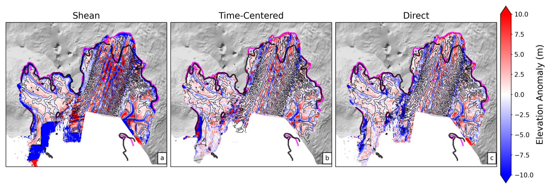
Figure A1 High-pass elevation anomaly for (a) the  Shean et al. (2019) DEM, (b) the time-centred DEM, and (c) the direct DEM. All plots are overlaid with the Shean et al. (2019) elevation anomaly zero contour lines in black.

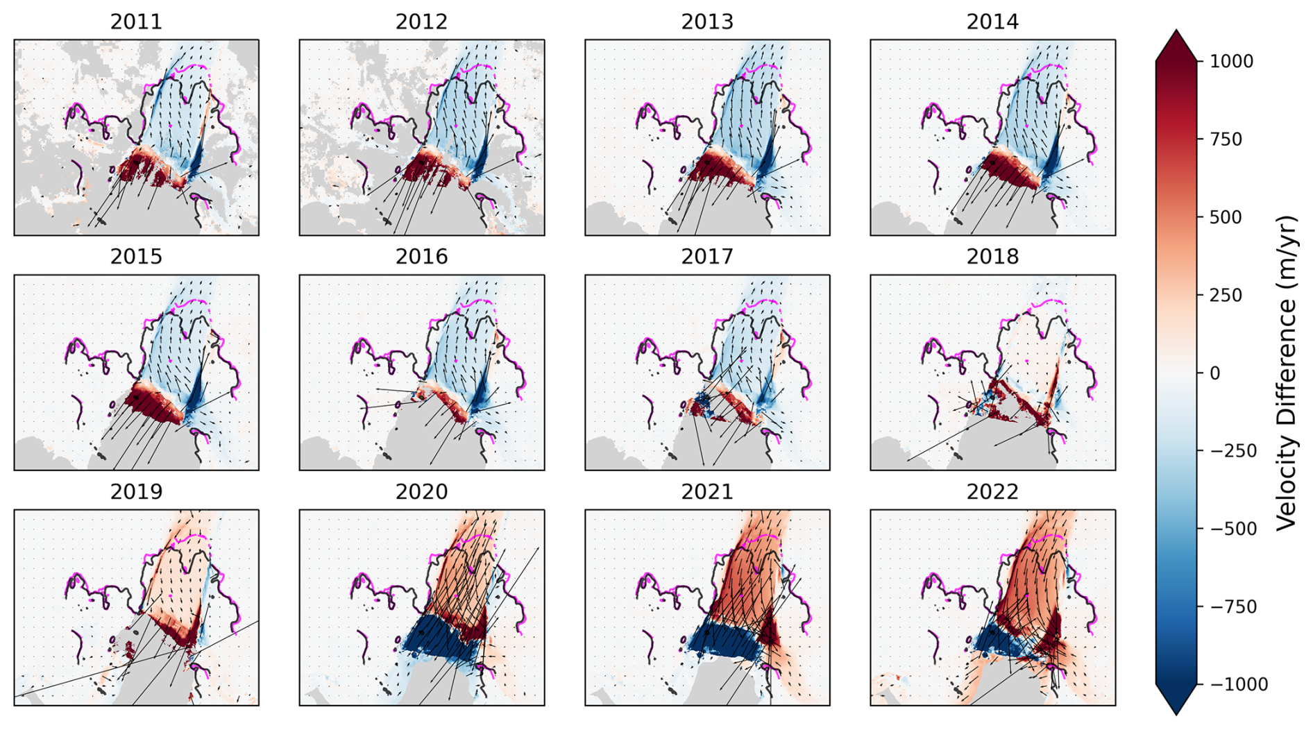
Figure A2 PIG annual velocity difference with the time averaged velocity over this period.

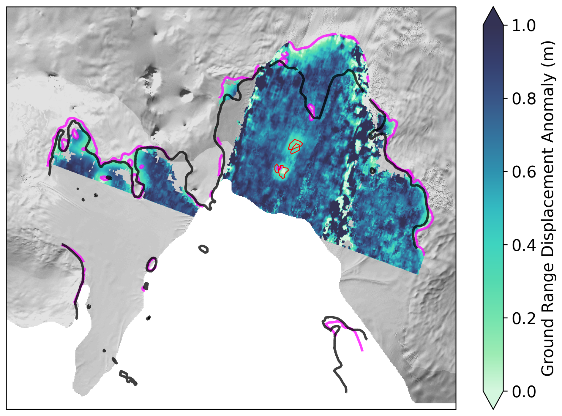
Figure A3 An example of the ground range vertical displacement anomaly as calculated by applying the DROT method to Sentinel-1 data. The red contour lines show the manually delineated areas of grounded ice. The data shown are calculated by comparing acquisitions from 27 January 2017 and 2 February 2017 with respective tide heights of 0.65 and 0.11 m.