Modeling the impacts of climate trends and lake formation on the retreat of a tropical Andean glacier (1962–2020)

Located in Peru's Cordillera Blanca, the Queshque Glacier (∼9.8° S) has experienced nearly continuous retreat since the mid-20th century. More recently, this trend has accelerated after the glacier transitioned from land to lake terminating. We use observations of glacier surface height change (1962–2008), bed topography, and climatology to evaluate the relative drivers of Queshque's evolution from 1962–2020. Six Open Global Glacier Model ensemble members differing in climatic sensitivity are calibrated to fit the mass balance rate of −442 ± 16 mm w.e. a⁻¹ calculated over the 2008 glacier area between 1962–2008. The models are then used to simulate monthly glacier mass balance over the entire study period and dynamic glacier evolution from 2008 to 2020. The models reproduce a typical outer-tropical glacier mass balance regime, showing continuous ablation throughout the year that increases during the pronounced wet season. Climatological trend analyses along with coupled mass balance and ice flow simulations indicate that temperature has been the predominant driver of mass loss since 2008 and that recent precipitation amounts have caused minor dampening of this trend. The strongest negative correlation between temperature and mass balance occurs during the wet season, while a positive correlation between precipitation and annual mass balance is most pronounced during the dry season. The influence of ENSO over mass balance trends appears to decline throughout the study period except during the wettest months, suggesting that wet season Pacific sea-surface temperatures are strong predictors of outer-tropical glacier mass balance variability. Finally, frontal ablation into the newly formed lake began in 2010. This caused ice acceleration at the glacier front, an average mass loss increase of 4 %, and a significant narrowing of the model ensemble mass loss spread. We conclude that while Queshque's trajectory remained coupled to climatic forcings, the new proglacial lake exacerbated and modified the retreat pattern regardless of the model climate sensitivity.

1 Introduction

Glacier-climate interactions in the tropics (23.5° S–23.5° N) have broad relevance across multiple timescales and applications (Mark, 2008). While tropical glaciers have varied considerably in size and extent during the Holocene (Stansell et al., 2023), they have retreated through most of the 20th and 21st centuries (Thompson et al., 2011; Vuille, 2018). Processes associated with these oscillations are of particular relevance in the Peruvian Andes, which host most of the world's extant tropical ice (RGI Consortium, 2017). The present article focuses on a glacier in Peru's Cordillera Blanca (CB), a mountain range that has been reworked by multiple phases of glaciation (Mark et al., 2024) but which has experienced nearly continuous glacier retreat since the 1920s (Burns and Nolin, 2014; Georges, 2004; Rabatel et al., 2013). Regional ice loss on the order of 29 % between 2000 and 2016 (Seehaus et al., 2019) has triggered cascading socioenvironmental repercussions spanning hydrographic shifts (Baraer et al., 2012; Bury et al., 2011; Mark et al., 2017) and changing geohazard exposure (Drenkhan et al., 2019; Huggel et al., 2020), among other challenges. On longer timescales, glacier extents have fluctuated in accordance with the evolving tropical Andean paleoclimatic conditions, producing records of Quaternary climate history through the discontinuous moraine record (Stansell et al., 2022) as well as through continuous geologic proxies of ice extent (Rodbell et al., 2008).

Whether for interpreting the tropical glacial geological record or understanding the trajectory of contemporary glacierized landscapes, disentangling the various drivers of glacier change is of primary concern. Like glaciers anywhere, those of the tropics and CB are controlled to the first order by the prevailing (hydro)climatological conditions (Kaser, 2001; Kaser and Georges, 1999). Superimposed on these dominant forcings, additional processes differentiate rates of change across timescales and between individual sites. These processes include climatic ones, most notably the South American Summer Monsoon (SASM) system, which brings moisture across the Andes from the Amazon basin on a seasonal basis (Vuille et al., 2008b; Zhou and Lau, 1998). Driven by the annual migration of the Inter-Tropical Convergence Zone and the related South Atlantic Convergence Zone (Kodama, 1992), the SASM produces stark hydroclimatic seasonality in outer-tropical latitudes, with over half of annual precipitation commonly occurring during DJF (wet-season) and negligible precipitation during JJA (dry-season). The El Niño-Southern Oscillation phenomenon (ENSO) modulates SASM strength while influencing temperature anomalies. The ENSO cycle is therefore a significant driver of inter-annual mass balance variability in the CB (Maussion et al., 2015; Vuille et al., 2008b).

Between individual glaciers, responses to climatic conditions are differentiated by morphometric factors such as hypsometry, aspect, and slope. Mass loss feedbacks associated with terrain radiation (e.g., Aubry-Wake et al., 2017) and glacial lake formation (e.g., King et al., 2018) further dictate retreat patterns independently from climate. This latter factor has been shown to be particularly significant at the mountain range scale, where lake versus land terminating glaciers may respond differently to uniform climatic conditions (Brun et al., 2019). To interpret glacier responses to climate change, it is thus often necessary to account for independent processes like lake formation alongside the climatic mass balance (e.g., Sutherland et al., 2020). A coupled mass balance and ice flow modeling approach is useful for parsing these diverse (climatic and non-climatic) influences over glacier change. Through transient simulations, coupled models can also facilitate interpolation between often discontinuous (paleo)glaciological observations.

However, tropical glaciers present persistent mass balance modeling challenges. One simple and common approach to glacier mass balance modeling is the temperature-index (TI) model, which is built on the empirical relationship between surface temperature and a glacier's ablation rate (Hock, 2003). While the TI approach tends to perform well in the mid-latitudes, its applicability is less obvious in the tropics where the sensible heat flux plays a diminished role and melt does not immediately correlate with the continuously low temperatures (Fernández and Mark, 2016). Although other approaches such as the enhanced TI (ETI) model exist (Hock, 1999; Pellicciotti et al., 2005), there are compelling justifications for using simple TI models within the tropics. First, a practical data limit: the more rigorous approach of physical energy balance modeling requires data which are not readily available at the spatiotemporal scale relevant to the topics outlined above. Moreover, temperature does tend to correlate with ablation on inter-annual to decadal timescales (Rabatel et al., 2013; Sicart et al., 2008), suggesting that a well calibrated TI model could theoretically internalize the numerous indirect impacts of temperature change (Ohmura, 2001).

The initial objective of our study is therefore to evaluate the performance of a coupled glacier mass balance and ice flow model using an empirical TI approach in an outer-tropical context. To do so, we present a case study of the CB's Queshque Glacier, simulating its evolution since 1962. Beyond offering an evaluation of our methodological approach, our analysis yields insight concerning the dominant (hydro)climatic processes influencing glacier mass balance trends in the outer-tropical Andes. Furthermore, it illuminates how the transition from land to lake termination has impacted rates of glacier retreat, irrespective of climate.

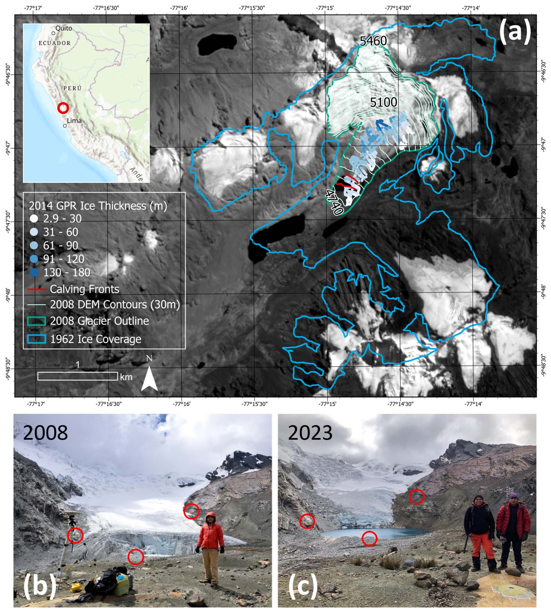
Figure 1 Location of Queshque Glacier on base imagery from 2023 (Sentinel 2). The position of calving fronts in 2018 and 2020 (derived from Sentinel 2 imagery) also shown. Inset basemap courtesy of ESRI (a). Field photos from 2008 (b) and 2023 (c) are marked with stable reference points for comparison. Note that the 2008 glacier outline delineates only ice that was considered in our model, excluding other glaciers that existed at the time.

2 Site Description

The Queshque Glacier (9.79° S, 77.25° W) is situated in the southern CB's Catac District and as of 2008, covered an area of 1.65 km² (Fig. 1a). From its headwall elevation of approximately 5460 m a.s.l., the glacier flows to the southwest, which provides optimal topographic shading, making it among the minority of glaciers in the range to retain a substantive ablation tongue. Located in the northern outer-tropical glacier region (Sagredo and Lowell, 2012), Queshque experiences the strong hydroclimatic seasonality described above and is therefore sensitive to fluctuations in the timing and intensity of moisture delivery by the SASM. While the glacier's 20th century retreat trend can be explained by significant warming (Mark and Seltzer, 2005), interannual mass balance variability is likely related to the ENSO cycle and SASM dynamics. The present study revisits the topic of mass balance forcings of Queshque Glacier, incorporating new data, observations, and improved numerical modeling to investigate both climatic drivers of ice loss and the impacts of transitioning from land to a lake terminating conditions.

We follow Queshque's retreat history over two periods: 1962–2008 and 2008–2020. Between 1962 and 2008, Queshque retreated over 1 km and ice coverage in the valley was dramatically reduced. From 2008 through 2020, the glacier retreated an additional ∼350 m and as of 2020, terminated at approximately 4800 m a.s.l. (Fig. 1). Retreat patterns after 2008 were modified by the onset of frontal ablation into a new proglacial lake. Proglacial lake formation occurred in two phases. First, after 1990 a small lake formed between the southern valley wall and the left lateral side of the glacier. By 2008, thinning and retreat had separated the glacier from this lake, but a till-covered bedrock knob continued to dam the water above the ice terminus elevation. The lake began draining towards the glacier, resulting in a mixture of outflow and meltwater pooling against the terminal ice (Fig. 1b). The second phase occurred after 2008, as further retreat revealed a significant overdeepening at the base of the glacier. Meltwater and outflow from the perched lake have continued to fill this overdeepening, forming a sizeable bedrock and till-dammed proglacial lake. As a result, lake calving became an observable component of total mass loss (Fig. 1c). By 2023, Sentinel 2 imagery shows that the lake had grown to about 300 m in width and 450 m in length, covering an area of approximately 100 500 m².

3 Data and Methods

3.1 Geodetic Mass Balance

A geodetic mass balance measurement between the dry seasons of 1962 and 2008 is derived by differencing digital elevation models (DEMs) from the respective years. Vertical aerial photographs taken on 12 July 1962 were used to produce a stereographic model of the glacier and surrounding terrain and extract a digital restitution of discrete point elevations over the glacier surface at a 30 m spacing using a Wild B8 analog plotter (Mark and Seltzer, 2005; following Brecher and Thompson, 1993). Points were then mapped to topographic contours at 25 m vertical resolution. Since the 1962 DEM was constructed using analog methods, we perform a quality comparison with a previously published digital version to guarantee the adequacy of the selected dataset. Huh et al. (2017) used the same imagery in ERDAS Leica Photogrammetry Suite version 11 software to construct a 10 m resolution DEM of the 1962 topography. Our comparison reveals considerable quality differences favoring our choice of DEM. We attribute quality concerns in the latter DEM to extremely low contrast in much of the accumulation zone that hampered the effectiveness of the DEM generation software. This resulted in obviously unnatural terrain artifacts that are absent from our chosen DEM product. A second DEM was produced using airborne light detection and ranging (LiDAR) data obtained in July 2008 (Huh et al., 2017). The LiDAR point cloud was converted to a 1 m resolution DEM covering the Queshque valley, used to delineate the 2008 ice boundary, then resampled to a courser 10 m resolution for use in the glacier model.

After aligning the DEMs using 3-dimensional coregistration (Figs. S1–S5 in the Supplement), we subtract the 1962 topography from that of 2008. We then calculate the specific (area averaged) mass balance (SMB) between 1962 and 2008 using projected pixels falling within the 2008 glacier boundary by Eq. (1):

$$\begin{array}{}\text{(1)}& \mathrm{SMB}={\displaystyle \frac{{\mathit{\rho }}_{\mathrm{water}}}{{\mathit{\rho }}_{\mathrm{ice}}}}{\displaystyle \frac{\mathrm{d}x\mathrm{d}y}{\mathrm{\Delta }t}}\sum _{i=\mathrm{1}}^n\mathrm{\Delta }{h}_i\end{array}$$

where dx and dy are the pixel resolution in the x and y dimensions of the local projection, Δt is the timespan in years, and Δh_i is the elevation change for a given pixel of the n pixels within the 2008 glacier boundary. ρ_water and ρ_ice are the densities of water and ice, taken respectively as 1000 and 900 kg m⁻³.

3.2 In-Situ Mass Balance Measurements

Ablation stake and snow pit data for Queshque Glacier are available between the years 2015 through 2019. The data comprise 11 individual point measurements spanning about 4700–5150 m in altitude that have been converted to water equivalence. Some measurements report altitudes occurring below the glacier terminus elevation in 2008. While lower altitudes in the stake data may be in part linked to glacier thinning, altitudes below the proglacial lake water level cannot be explained in this way. It appears, rather, that some level of inaccuracy or negative bias exists in the elevation data. We therefore apply a uniform bias correction of 26 m across all elevations reported in the stake data such that the lowest stake measurement reaches 4727 m, which is the elevation below the glacier terminus in 2008 (see Sect. 3.5.3). We recognize that this correction is a source of considerable uncertainty, however, we determined it to be necessary since we lack additional GPS metadata. Due to inconsistencies in the duration of the stake measurements, ablation measurements were converted to m w.e. d⁻¹ then multiplied by 365 d to arrive at standard units of m w.e. a⁻¹. Ablation stake data are reserved for validation purposes.

3.3 Glacier Bed Topography and Ice Thickness

A ground penetrating radar (GPR) survey using 10 MHz frequency was conducted over the Queshque Glacier tongue during the dry season of 2014 using the Radar HF from Unmanned Industrial LDTA (Fig. 1a). Coordinates and surface elevations associated with the radar scans are established by averaging values from two GPS receivers. We interpreted radar scans visually using RadarView 1.0 software and determined thickness profiles based on first reflectance. These values were subtracted from the GPS ice surface heights to derive the bed topography. We calculated ice thickness in 2008 (derived thickness) by subtracting the bed topography from the 2008 DEM (Fig. S6). We then randomly divided the 2014 GPR survey into equally sized calibration and validation datasets before downscaling the respective subsets by averaging observations located within the same 10×10 m grid cell. This aggregation method facilitates comparisons between ice thickness observations and models without altering the spatial patterning of the GPR data (Pelto et al., 2020).

To ensure the accuracy of our derived thickness measurements, we evaluate them against a minimal GPR transect surveyed in 2009 (Stansell et al., 2022). For each point observation from the 2009 transect, we average the values from the four closest grid cells that contain derived thickness measurements. We then evaluate derived ice thickness error (derived minus observed thickness) on a point-by-point basis. Error ranges from 13 to −15 m, with a single outlier of −28 m (Fig. S7). Excluding the outlier, the datasets show strong agreement, with respective root mean squared error (RMSE), mean absolute error (MAE), and mean error (ME) values of 7, 5, and ∼0 m. While we would expect to detect modest (<0.5 m) thinning in the ablation zone between 2008 and 2009, the resolution of the GPR datasets may preclude this observation. An elaboration of the GPR validation process is provided with the Supplement.

3.4 Climatology

The SENHAMI-HSR-PISCO (hereafter PISCO) monthly gridded temperature, precipitation, and fixed gridded reference altitude datasets are adopted for the period 1980–2020 (Aybar et al., 2020; Huerta et al., 2023). Mean monthly temperatures are estimated by averaging the average minimum and maximum daily temperatures for each month. The PISCO climatology is extended to January 1960 using monthly temperature and precipitation standard anomalies from the downscaled Climate Research Unit (CRU) dataset (Harris et al., 2014; New et al., 2002). Both the PISCO and CRU datasets showcase typical outer-tropical Andean features, with stark precipitation seasonality (nearly all precipitation occurring during the austral summer) and only slight seasonal variation in temperature (Fig. S8). Despite its higher spatial resolution, PISCO runs a local warm bias as compared to a completely overlapping timeseries from CRU. Temperature and precipitation bias correction are addressed during the mass balance model calibration.

3.5 Glacier Model

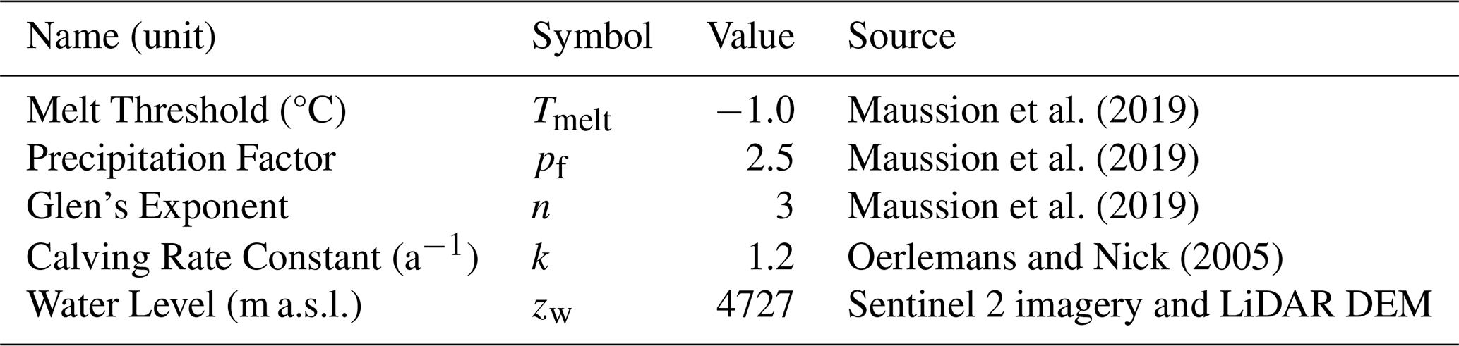
To evaluate drivers of glacier mass change and ice loss, we employ mass balance, ice flow, and calving models from the Open Global Glacier Model (OGGM) version 1.6.1 (Maussion et al., 2019). All simulations begin from the glacier state in 2008 and leverage the elevation band approach to create a flowline-based representation of the glacier (Huss and Farinotti, 2012; Huss and Hock, 2018). The glacier is divided into equally spaced elevation bands at 20 m intervals (half the resolution of the underlying map) and mean glacier attributes are calculated per band, beginning with elevation, width, area, and slope, all of which are derived from the 2008 DEM and glacier outline. Calibration of the model components is described below. Constant and calibrated parameters are listed respectively in Tables 1 and 2.

3.5.1 Mass Balance Model Ensemble

We employ the OGGM's monthly TI scheme using the extended PISCO climatology. The mass balance m during month i at elevation z is computed as:

$$\begin{array}{}\text{(2)}& m_i\left(z\right)=p_{\mathrm{f}}{P}_i^{\mathrm{solid}}\left(z\right)-\mathit{\mu }max\left((T_i\left(z\right)+{\mathit{\epsilon }}_T)-T_{\mathrm{melt}},\mathrm{0}\right)\end{array}$$

where $P_i^{\mathrm{solid}}\left(z\right)$ and T_i(z) are the monthly solid precipitation and average monthly temperature at a given elevation, T_melt is the temperature above which melt can occur, and μ is a positive degree-day factor (DDF; Hock, 2003). We assume orographic precipitation enhancement to be uniform across the glacier, allowing us to use a single precipitation factor (p_f) to scale P_i from the gridded climatological dataset. Lacking meteorological data to identify the “correct” p_f parameter, we opt for a default value of 2.5, which is commonly adopted when using the CRU gridded precipitation product in glaciological applications (Marzeion et al., 2012; Maussion et al., 2019). All precipitation is assumed to be frozen when T_i(z)<0 °C and liquid when T_i(z)>2 °C. At intermediate temperatures, the proportion of solid to liquid precipitation is scaled linearly. T_i(z) is calculated using a lapse rate of −6.5 °C for each km difference in altitude between a given point on the glacier and the climatology's reference altitude of 5111 m. Due to the warm bias identified previously, temperature is further reduced by a negative temperature bias parameter (ε_T). We note that lapse rates in the tropical Andes are a critical, yet highly uncertain parameter in tropical glaciological studies. Temperature sensor networks in the Cordillera Blanca, as well as atmospheric modeling using the WRF, show that regional lapse rates are seasonally variable, increasing in magnitude during the dry season. Measured lapse rates vary from $\sim -\mathrm{9.1}$ to $\sim -\mathrm{6.0}$ °C km⁻¹ between seasons, while modeled lapse rates varied from $\sim -\mathrm{7.5}$ to $\sim -\mathrm{5.8}$ °C km⁻¹ (Hellström et al., 2017). One limitation of our model is that it cannot incorporate seasonal lapse rate variability during the mass balance model calibration, despite this playing a potentially crucial role in the tropical Andes. A compromise between the measured and modeled seasonal extremes was therefore selected and we opted for the conventional −6.5 °C km⁻¹ for the sake of consistency and comparability with other studies.

Annual modeled SMB is calculated by averaging the area weighted elevation band mass balance per month. Three free parameters, ε_T, μ, and p_f are calibrated by fitting modeled mass balance between 1962 and 2008 to the observed geodetic SMB. To do so, we first determine reasonable ε_T values using a simple sensitivity test requiring that temperatures fall to ≤0 °C for a significant duration each year at the altitude range of the glacier. Following the results of this test, we vary ε_T by increments of 0.5 °C between −9.0 and −6.5 °C then calibrate μ under each temperature bias to fit the SMB from 1962 to 2008. If the model cannot converge on a DDF satisfying the constraint on SMB, p_f is subsequently calibrated. This procedure produces six mass balance models with differing variances (climatic sensitivities), but uniform mean SMB during the calibration period. Because each subsequent modeling step depends on the mass balance parameters, the six parameter sets become the basis for a model ensemble used in the remainder of the study. To evaluate the relationship between ensemble mean glacier mass balance variability, temperature, precipitation, and ENSO, we first use the Mann-Kendall test to evaluate significant (p<0.05) linear trends in the climate and ensemble mean SMB timeseries. To facilitate comparison with ENSO indices, we detrend and normalize all climate and mass balance variables by fitting them to 3rd order polynomials, subtracting the polynomial from the respective timeseries, then dividing the detrended data by their standard deviations (Dabernig et al., 2017; Wu et al., 2007). We then use Pearson correlations to compare the normalized SMB and climate timeseries to the ENSO indices including Niño-3.4, the Oceanographic Niño Index (ONI), the Southern Oscillation Index (SOI), and their seasonal values.

3.5.2 Glacier Thickness and Flow Model

The GPR dataset is leveraged to calibrate the ice flow model by minimizing error between modeled and observed ice thickness. We compute initial (2008) glacier ice thicknesses for each ensemble member following a well-documented continuity approach that leverages the calibrated mass balance models (Farinotti et al., 2009; Maussion et al., 2019). OGGM first evaluates the “apparent mass balance” ($\stackrel{\mathrm{̃}}{m}$) per elevation band by assuming steady-state conditions (SMB =0). Ice flux (q) at each band is then calculated as the cumulative apparent mass balance from the area (a) above a given altitude (z). By continuity, we can assume that flux as cumulative mass balance above a given elevation band is balanced by ice flowing out of the band. OGGM therefore sets cumulative mass balance equal to ice flow using the shallow ice approximation (Hutter, 1981):

$$\begin{array}{}\text{(3)}& q=\underset{z}{\overset{z_{\max }}{\int }}\stackrel{\mathrm{̃}}{m}\mathrm{d}a=S\times {\displaystyle \frac{\mathrm{2}A}{n+\mathrm{2}}}h{\left({\mathit{\rho }}_{\mathrm{ice}}gh\mathit{\alpha }\right)}^n\end{array}$$

where z_max is the maximum glacier altitude, S is elevation band width, g is the acceleration due to gravity, α is surface slope derived from the 2008 DEM, and h is ice thickness. A and n are the creep parameter and exponent from Glen's flow law, which describes the deformation of polycrystalline ice (Glen and Perutz, 1955). We adopt the conventional n=3, and leave A as a free parameter. While total ice movement results from the combination of deformation (“creep”) and basal sliding, data scarcity limits our ability to estimate sliding. We therefore assume that all flow arises from deformation. As a result, it is likely that our models overestimate the magnitude of deformation while accurately predicting ice flux (Pelto et al., 2020).

OGGM performs a glacier ice thickness inversion by solving Eq. (3) for h at the center of each elevation band and extrapolating ice thickness by assuming a parabolic bed shape. The steady-state assumption can often lead to overestimated mass flux and therefore exaggerated overdeepenings located near the base of the glacier. To address this and achieve realistic proglacial lake depths, we set a minimum slope parameter of 7.5°, which clips the glacier surface slope to ≥7.5° during the ice thickness inversion process, resulting in the flattest sections of ice retaining higher flow rates. This is necessary because otherwise the model will overestimate ice thickness to satisfy mass continuity with the steeper slopes above. The minimum slope parameter was determined after a series of sensitivity tests examining the impact of this parameter on terminus ice thickness, which, following sufficient glacier retreat, translates to eventual proglacial lake depth. In summary, this parameter decision increases ice velocity at the expense of thickness and aids to replicate observable ice dynamics.

We calibrate the A parameter during the inversion by minimizing ME in ice thickness against the GPR calibration dataset. Because the inversion is sensitive to the mass balance parameters, A is calibrated individually for each of the model ensemble members. During calibration, the parameter is adjusted to ensure that modeled ice thickness matches observations despite different ablation rates across models. The ablation rates themselves are a product of the DDF, which is directly influenced by the model temperature bias. The calibrated creep parameters are therefore direct outcomes of the previous mass balance calibration step. After identifying an optimal A parameter for each member, we evaluate the resulting ice thickness map for ME and MAE against the GPR validation dataset.

For dynamic glacier simulations, we use the OGGM Flux-Based model based on Glen's flow law. For each model ensemble member, we therefore adopt the respective A parameter calibrated during the inversion and continue to neglect sliding.

3.5.3 Calving Model

The OGGM implements a simple scheme developed by Oerlemans and Nick (2005) for calculating the calving flux (q_calving) at lake terminating glaciers:

$$\begin{array}{}\text{(4)}& q_{\mathrm{calving}}=kd{h}_{\mathrm{f}}w\end{array}$$

where k is a calving rate constant, h_f is ice thickness at the calving front, and w is the width of the calving front. The d parameter is the water depth calculated from the water level (z_w) and bed altitude at the glacier terminus (z_b) as:

$$\begin{array}{}\text{(5)}& d=z_{\mathrm{w}}-z_{\mathrm{b}}\end{array}$$

while z_w may vary on a seasonal basis, an examination of Sentinel 2 imagery shows negligible variation in the ice distal extent of surface water between the small pool visible in 2008 and the sizeable lake present in 2020. We therefore adopt the LiDAR DEM altitude at the site of pooling in 2008 as a constant z_w throughout the duration of the study. z_b is adjusted each month based on the position of the calving front and k is adopted from a low-end estimate used in previous work (Table 1). Although this parameter could be calibrated to match observed glacier terminus positions, calving fluxes, or other metrics, we opt to maintain a general parameterization across all models. This decision ensures that calving model performance is not the result of calibration and instead reflects the impact of the process of frontal ablation on glacier retreat dynamics.

Table 1 Constant model parameters used in Eqs. (1)–(5).

3.6 Glacier Evolution Experiments

We run four dynamic ice flow modeling experiments to evaluate the relative drivers of ice loss from 2008 through 2020. To isolate the impact of frontal ablation, we force the glacier to evolve with and without lake calving under the historical climatology (Sect. 3.3), for which we take the PISCO dataset between 2008 and 2020. The two additional experiments both neglect calving and isolate the temperature versus precipitation forcings by maintaining the monthly climatological temperature or precipitation levels as recorded during the first 30 years of the mass balance record (1962–1991). Experiments are performed independently for each of the six model ensemble members and the results are validated against glacier surface velocity measurements representative of 2017–2018 (Millan et al., 2022).

3.7 Glacier Terminus Positions

Direct comparison of glacier terminus position (glacier length) to satellite imagery is complicated by the elevation band flowline method selected in this study. Although this method facilitates certain analyses such as comparisons of modeled and observed surface velocity, it limits OGGM's accuracy concerning glacier length (Maussion et al., 2019 and online documentation). To circumvent this limitation, we have instead opted to estimate glacier length from 1962–2023 based on the elevation of the 2008 DEM where it intersects historical glacier terminus positions derived from aerial imagery, Landsat 8, and Sentinel 2 satellites (Fig. S9). This is a more reliable approach for aligning modeled and observed glacier positions, as the elevation band flowline is built around the 2008 DEM. After identifying terminus surface altitudes with respect to the 2008 DEM (Fig. S10), we then locate the point along the elevation band flowline corresponding to the terminus position of each given year. To do so, we query the elevation band flowline such that the glacier surface elevation in 2008 is within ± 2 m of the calculated terminus elevation of a given year since 2008. This small range accounts for the fact that not every possible elevation is included as an index in the elevation band model. The resulting glacier terminus position timeseries can then be directly compared to the glacier evolution experiments described in Sect. 3.5. For further details regarding the construction of this timeseries, refer to Sect. S1.4 in the Supplement.

4 Results

4.1 Mass Balance Model Calibration and Validation

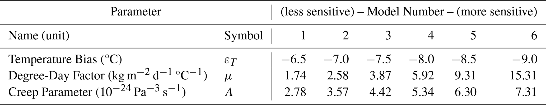
After aligning the 1962 and 2008 DEMs through 3-dimensional coregistration (see Sect. S1.1), differencing the DEMs shows that Queshque experienced a SMB rate of −442 ± 16 mm w.e. a⁻¹ between the two periods. This value provides a constraint on mean modeled SMB for each ensemble member throughout the calibration period, resulting in higher μ (DDF) as ε_T becomes more negative (Table 2). As a result, models with less negative ε_T have less interannual SMB variability and we can therefore characterize them as lower climate sensitivity models. Alternatively, high magnitude (more negative) ε_T models showcase greater variability, or more exaggerated responses to the same variations in climate. We therefore characterize models with lower DDF parameters as less sensitive, and those with higher DDF parameters as more sensitive (Table 2). As such, model 1 is considered to be the least sensitive of our ensemble, while model 6 showcases greatest sensitivity. We note that this variation in sensitivity is a result of calibration, as models with less negative temperature biases are subject to warmer temperatures and therefore must have more muted responses to climate warming in order to fit the long-term geodetic mass balance. Furthermore, we note that additional parameter uncertainty exists in our fixed mass balance parameters, particularly T_melt (Pellicciotti et al., 2008), but also derives from neglected processes such as avalanching. However, DDF calibration procedure should theoretically compensate for these uncertainties by matching long-term mass balance observations (Maussion et al., 2019).

Although modifying the p_f parameter leads to intuitive changes in climate sensitivity (higher values increasing sensitivity to temperature as compensation), doing so does not provide additional insight into the mass balance regime. Moreover, all models converged on DDF values fitting the observed SMB without needing to alter the default precipitation factor. We recognize, however, that this parameter is highly uncertain, as very few reliable accumulation records exist from the tropical Andes. Our direct, though limited in duration, mass balance measurements introduced in Sect. 3.2 record accumulation as high as 1.95 m w.e. a⁻¹ at an elevation of 5150 m on Queshque Glacier. Using the precipitation factor of 2.5, our mass balance models produce average annual accumulation rates of 1.9 ± 0.4 m w.e. a⁻¹. This value is consistent with the limited direct accumulation measurements we have available. In contrast, the nearby Huascarán Col experiences lower annual accumulation of about 1.4 m w.e. a⁻¹ (Thompson et al., 1995; Weber et al., 2023). Although the default precipitation factor of 2.5 does seem to produce realistic accumulation values for Queshque Glacier, we note that changes in this parameter do not introduce bias into the mass balance model so long as the DDF is recalibrated, as we have done in the present study (Maussion et al., 2019).

Table 2 Calibrated model parameters used in Eqs. (2)–(3) for six-model ensemble.

To assess mass balance model performance, we perform two validation analyses against the ablation stake data. First, we consider the magnitude of ablation in the lower altitudes (defined as 4800 m and below) of the ablation zone as a constraint on the realistic melt rates near the glacier terminus. We then consider the observed ablation gradient in comparison to our models.

4.1.1 Magnitude of Ablation

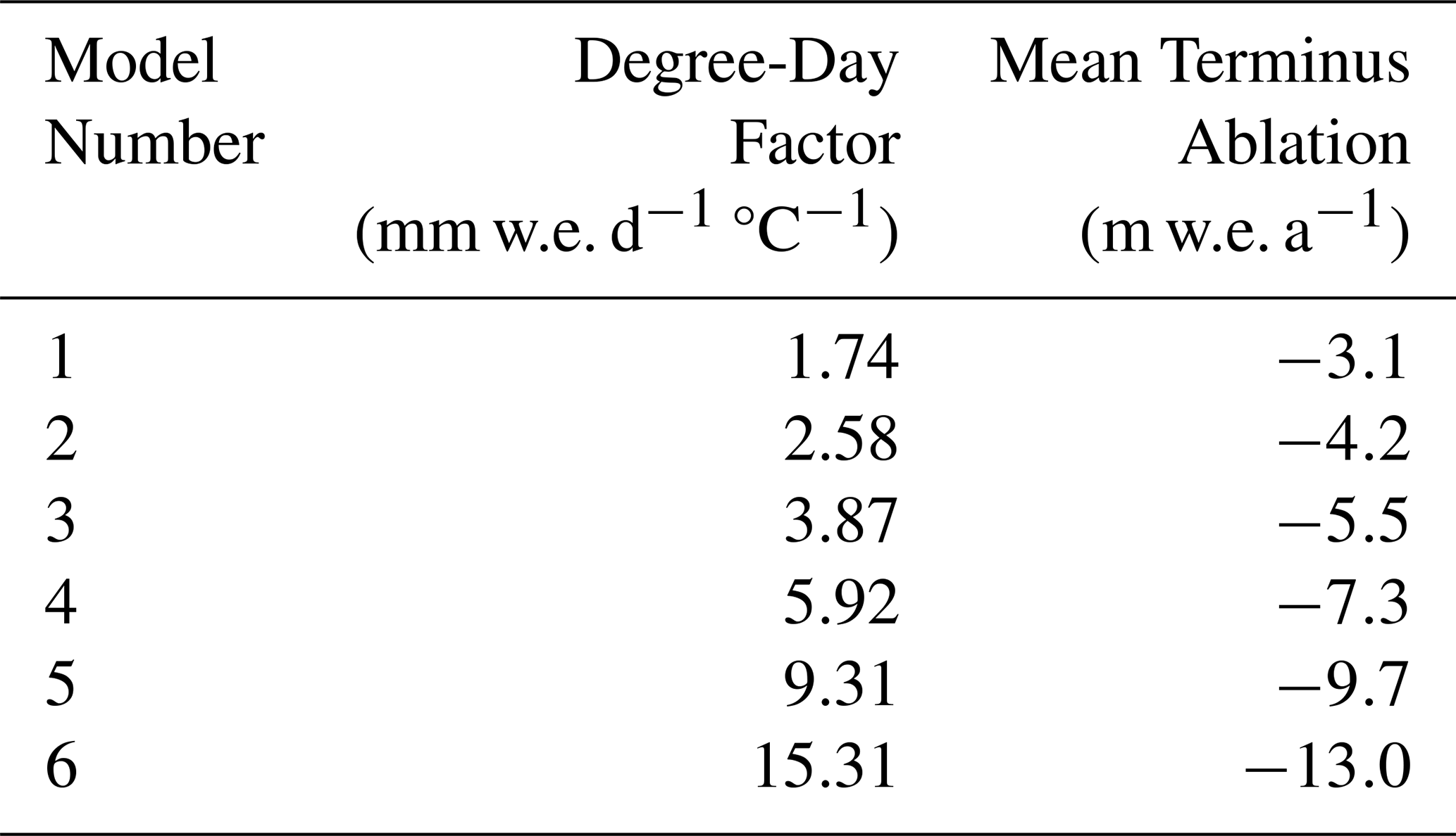
Observed annual melt rates below 4800 m range from about −11.4 to −3.5 m w.e. a⁻¹, averaging at 7.5 m w.e. a⁻¹. Melt rates are greatest during the El Niño year of 2016, which is consistent with our simulation of overall specific mass balance. This range provides a limit on the magnitude of ablation we should expect to obtain near the glacier terminus. Average modeled ablation rates at the lowest altitudes during the years 2015 through 2019 are presented in Table 3. We find that models 2, 3, 4, and 5 fall within the bounds of observations, with model 4 producing ablation rates closest to the observed mean.

Table 3 Mean annual ablation produced by each model at the lowest altitudes (4727–4800 m) during the years 2015–2019 which coincide with the timespan of in-situ mass balance measurements. The degree-day factors are included for reference.

4.1.2 Ablation Gradient

Although our models can reproduce the observed ablation rate at the glacier terminus, we find that their ability to reproduce the observed ablation gradient is limited. Fitting a linear trend to all negative stake observations, we calculate that on average ablation decreases (becomes less negative) by 8.5 mm w.e. d⁻¹ for every 100 m gain in elevation. By dividing this value by the lapse rate of −0.65 °C per 100 m, we arrive at an estimated temperature sensitivity (degree-day factor) of approximately 13 mm w.e. d⁻¹ °C⁻¹. Based on the maximum lapse rate seasonality identified by Hellström et al. (2017), we note that this value could range between 9.3 and 14.6 mm w.e. d⁻¹ °C⁻¹. However, our model mass balance calibration was performed under the assumption of seasonally consistent lapse rate, and we therefore adopted the conventional value.

To ensure that our model matches the observed ablation gradient, we recalibrated the model by adjusting the temperature bias to fit the observed geodetic mass balance using a fixed temperature sensitivity parameter (DDF) of 13 mm w.e. d⁻¹ °C⁻¹. This DDF falls between models 5 and 6 (Table 3). We find, however, that this calibration overestimates the ablation rate at the glacier terminus (Fig. S11a). We next introduce an additional temperature bias, cooling the model until it approximates the observed average mass balance profile in both magnitude of accumulation and ablation, and the mass balance gradient. We find, however, that this model vastly overestimates the specific mass balance and would indeed induce glacier growth since 1962 (Fig. S11b). To further investigate the threshold between glacier growth and retreat, we conduct a sensitivity experiment wherein the fixed-gradient model is cooled until balanced conditions are achieved between 1962 and 2008. The results indicate that if forced to match the observed ablation gradient, all stake observations except from the extreme El Niño year of 2016 show a more positive mass balance than would be required to model balanced conditions (Fig. S11).

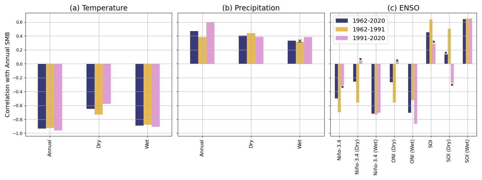
Figure 2 Correlations for annual, dry-season (JJA), and wet-season (DJF) detrended temperature (a), precipitation (b), and ENSO indices (c) with the detrended annual SMB ensemble mean. Insignificant correlations (p>0.05) are marked by crosses.

4.2 Climate and Mass Balance Variability

Over the course of the mass balance simulation period (1962–2020), mean annual temperature (MAT) rose by approximately 0.15 °C per decade based on a simple linear regression, with dry-season temperatures rising faster and more consistently than during the wet-season (Fig. S12a). While we detect no significant trend in total annual precipitation (TAP), a moderate, though statistically insignificant drying (wetting) trend is present during the dry (wet) season (Fig. S12b). These trends were associated with a model ensemble average SMB decline of approximately −221 mm w.e. a⁻¹ per decade by 2020.

After detrending the SMB and climatological timeseries, we find that SMB is tightly correlated with MAT ($r=-\mathrm{0.93}$) (Fig. 2a). TAP maintains a moderate correlation with SMB throughout the simulation, increasing after 1991 to a correlation coefficient of 0.59. Correlations also suggest that SMB is slightly more closely linked to dry season than it is to wet season precipitation (Fig. 2b). Regarding ENSO, the most consistent predictor of annual mass balance is the wet-season Niño-3.4, which retains a strong anticorrelation with SMB throughout the duration of study ($r<-\mathrm{0.70}$). While annual Niño-3.4 values serve as a moderate SMB predictor during the first 30 years after 1962, this relation appears to dampen over time, becoming insignificant in the latter 30-year period. Alternatively, negative correlations with the wet-season ONI index reaches −0.86 in the last 30 years of the study period. Other ENSO indices appear to reverse in the sign of their correlation with SMB over the course of the study. Most notably, the dry season SOI index maintains a moderate positive correlation with SMB for the first 30 years before switching to a low to moderate (though not statistically significant) negative correlation after 1991 (Fig. 2c). Correlations are considered significant when p<0.05.

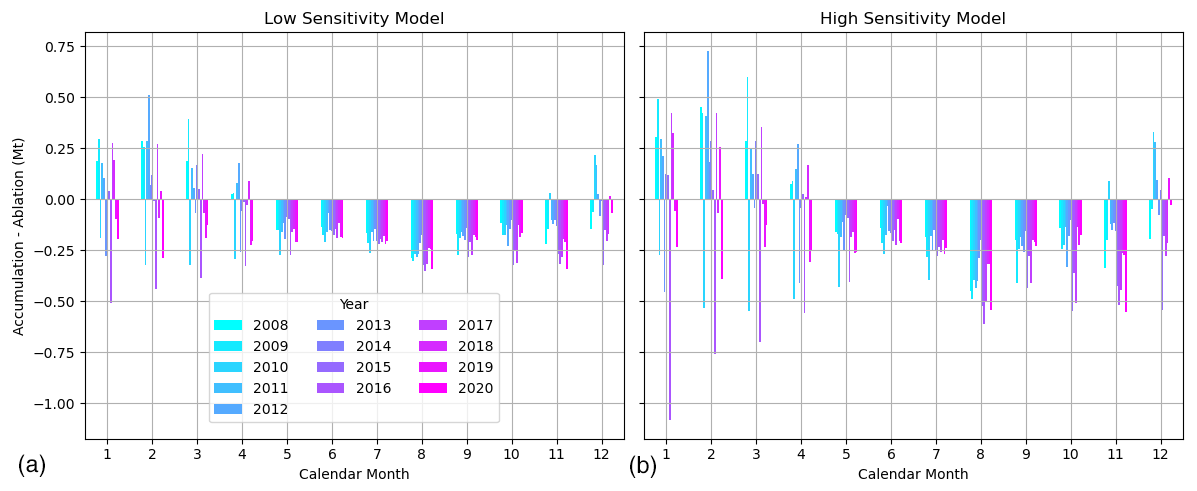
Figure 3 Net mass balance as accumulation minus ablation for each month of each year (2008–2020). The low (a) and high (b) sensitivity models correspond to model numbers 2 and 5, respectively.

4.3 Climate and Mass Balance Seasonality

We evaluate monthly accumulation and ablation variability between 2008 and 2020, showing that the model reproduces an archetypical tropical glacier mass balance regime. Accumulation, taken as the total solid precipitation to fall on the glacier each month, follows the pattern controlled by the SASM. Across all models, 53 %–56 % of accumulation between 2008 and 2020 fell during the core wet season (DJF), while less than 2 % occurred in the core dry season of JJA (Fig. S13a). Following a similar though less pronounced pattern, 27 %–32 % of all ablation occurred during the wet season, while 19 %–22 % occurred in the dry season (Fig. S13b). Together, this seasonality produces a mass balance regime wherein ablation occurs continuously throughout the year but enhances during the wet season when virtually all accumulation occurs. As a result, the model produces consistent negative mass balance between May and November, with the exception of November 2010, which had a slight positive balance due to above average accumulation and below average temperature. Both positive and negative mass balance months occur between December and April and the net balance magnitudes are greater during this time (Fig. 3). As model sensitivity increases, accumulation and ablation seasonality are amplified, and net balance becomes increasingly variable.

4.4 Glacier Volume and Thickness Estimates

Due to the ice thickness inversion procedure's dependence on the mass balance parameters, the inverted bed topography differs across models, leading to differences in initial total glacier volume. Below 5100 m, however, ice thickness is constrained by the GPR observations. Model results at lower elevations are therefore consistent to one another, with mean thickness ranging negligibly between 73.5 and 73.6 m. Error against the validation GPR dataset is also consistent, with approximately 30 cm ME and 24–25 m MAE (Table 4). These metrics imply that while ice thickness at any given point is likely to be over or underestimated by about 25 m, the average ice thickness and therefore glacier volume is well constrained. This level of accuracy is comparable to similar work using GPR (Pelto et al., 2020). By contrast, observations are lacking in the accumulation zone, and ice thickness varies across models. Initial modeled ice volumes range from 7.7–8.1×10⁷ m³, reducing as climatic sensitivity increases. Volume differences across models are mostly attributed to ice thickness differences in the accumulation zone. Relatedly, the calibrated creep parameter, A, increases with greater climate sensitivity, reflecting enhanced ice flux (Table 2).

Table 4 Ice thickness inversion results for each model ensemble member.

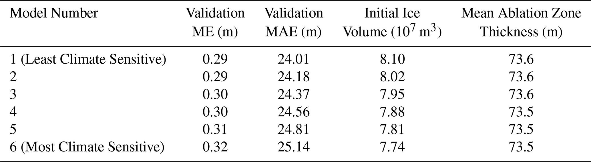
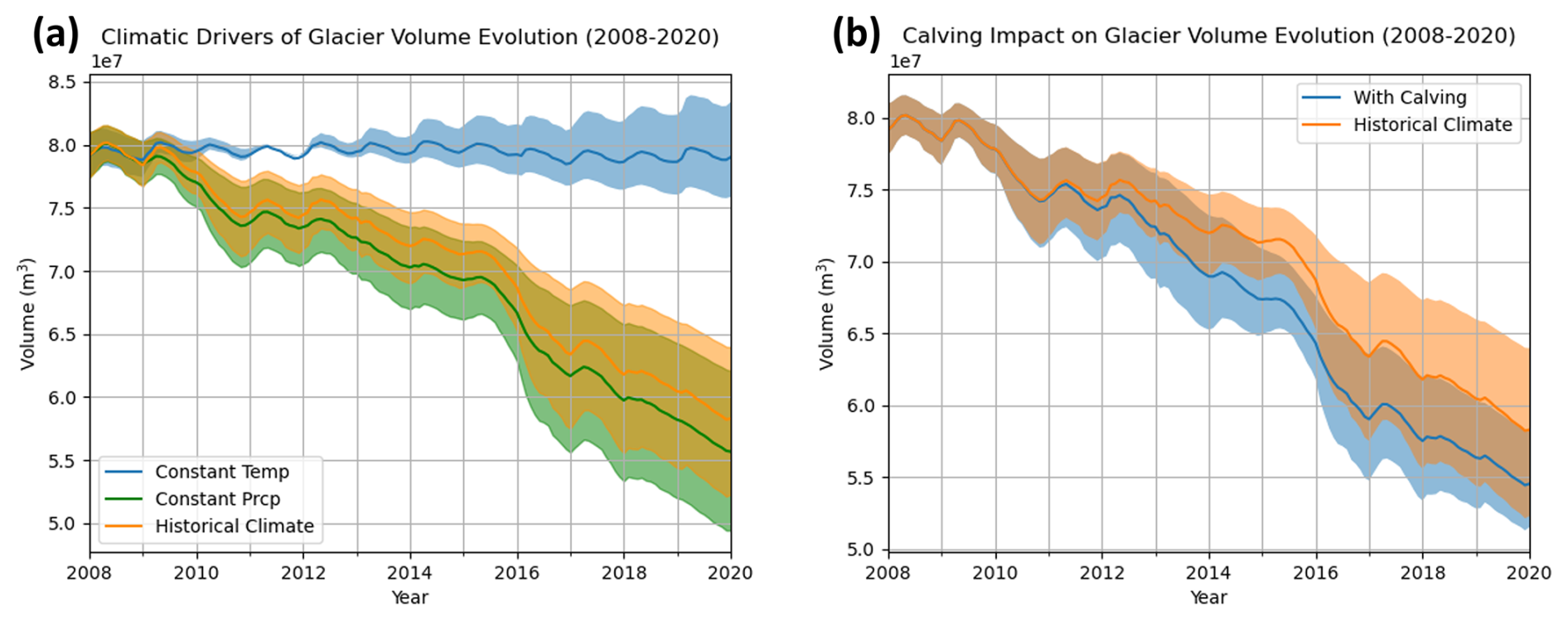
Figure 4 Comparison of dynamic glacier evolution under the historical climate, constant climatological mean temperature, and constant climatological mean precipitation (a). Comparison of glacier evolution under the historical climate conditions with and without including frontal ablation (b). Solid lines represent ensemble mean values and shaded regions indicate the ensemble spread.

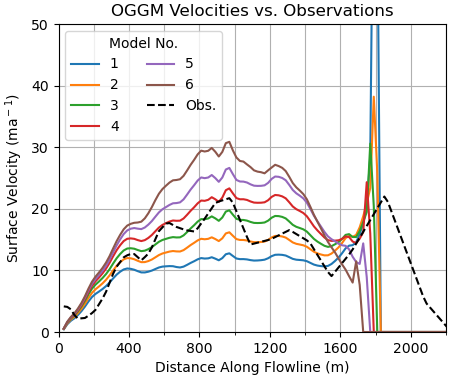
Figure 5 Surface velocity profiles of the 6-member model ensemble. Each profile is representative of mean altitude-binned values. Observations (Obs.) come from Millan et al. (2022). Modeled velocity falls to zero at glacier terminus whereas observations reduce more gradually, owing to satellite image resolution and potentially the presence of ice mélange.

4.5 Ice Dynamics

The four glacier evolution experiments isolate different mass balance forcings, enabling us to parse their relative influences over glacier dynamics. Forced by the real-time monthly conditions recorded over the study period in the PISCO dataset, the ensemble mean glacier volume reduces by 26 ± 6 % between 2008 and 2020. Holding monthly precipitation to 1962–1992 climatological means derived from the combined CRU-PISCO dataset while retaining the monthly PISCO temperature values results in a similar trend with heightened volume loss of 30 ± 6 %. Alternatively, driving the model with climatological temperature and real-time monthly precipitation yields a nearly steady-state ice volume oscillating around the ensemble initial conditions of $\mathrm{7.9}\pm \mathrm{0.1}\times {\mathrm{10}}^{\mathrm{7}}$ m³, with more climatically sensitive models producing net glacier growth of up to nearly 8 % (Fig. 4a). Finally, incorporating the effects of proglacial lake formation by implementing frontal ablation accelerates mass loss beginning in 2010 and produces a narrower model spread of 28 %–33 % volume loss by 2020, constituting 0.4×10⁷ m³ of additional volume loss (Fig. 4b).

A comparison between elevation band average modeled and observed surface ice velocity profiles suggests that the model produces realistic local ice dynamics. Both models and observations show glacier surface velocity in 2018 increasing from a minimum at the beginning of the elevation band flowline (the top of the glacier), peaking at around 900 m downstream, then decelerating. Surface velocities spike again at the calving front (Fig. 5). In terms of magnitude, models 2, 3, and 4 stay truest to observed velocities, showing RMSE values below 4 ma⁻¹ (Table S1 in the Supplement), though each overestimates the peak velocity at the glacier terminus. Note that the superior performance of models 2, 3, and 4 is consistent with the mass balance model validation presented in Sect. 4.1.1. This is unsurprising, as the magnitude of ablation is related to overall ice flux, which controls surface velocity. An apparent positive terminus velocity bias is present in most models, which is likely related to the impact of lake depth on calving flux.

When calving is excluded from the glacier evolution experiments, higher climate sensitivity ensemble members retreat faster than their low sensitivity counterparts. The addition of a calving mechanism impacts all ensemble members but reduces the ensemble variance by disproportionately accelerating the retreat of lower sensitivity models (Figs. 4, 6). Furthermore, the inclusion of calving results in much greater agreement between modeled and observed ice terminus positions. By 2020, the modeled glacier calving positions show close alignment with independent observations (Fig. 6a), though performance quality differs from year to year. Specifically, it appears that our models exaggerate frontal retreat rates by 2018 (Fig. 5) but slow to match observations by 2020 (Fig. 6). By 2020, the higher sensitivity models retreat to a greater extent than their less sensitive counterparts. However, differences between models with calving are reduced as compared to when neglecting this process (Fig. 6).

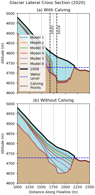
Figure 6 Details of the glacier lateral cross section in 2020 produced by each model ensemble member with (a) and without (b) calving. The observed ice surface in 2008 is depicted in bold black and referential calving front positions are depicted as vertical dashed lines. Note that the x and y axes are not to scale, and that the first 1000 m of the glacier are excluded to highlight differences at the glacier terminus.

5 Discussion

5.1 Tropical Glacier Mass Balance: Major Components Reproduced in TI Model

From a climatological perspective, the distinguishing feature of the outer-tropical glacier mass balance regime is the absence of strong thermal seasonality coupled with pronounced seasonal differences in precipitation (Kaser and Osmaston, 2002). This leads to continuous ablation throughout the year, with accumulation confined almost exclusively to the wet season. The magnitude of ablation, however, is controlled by processes governing the net radiation balance and the partitioning of energy available for melt (Hastenrath, 1997). Multiple factors influence this partitioning, but they generally result in an archetypical outer-tropical Andean glacier seasonality featuring enhanced ablation during the wet season (Kaser and Georges, 1999). Glacio-hydrological observations at Yanamarey and Uruashraju in the CB support this theory, showing that net accumulation occurred only during JFMAM, and JFMA, respectively (Mark and Seltzer, 2003). Further confirmation is offered by process-based surface energy balance (SEB) models applied on glaciers in the CB (Fyffe et al., 2021) and Bolivia's Zongo Glacier (Sicart et al., 2005; Wagnon et al., 1999) which show that energy for melt typically increases during the wet season. An exception to this rule has been observed at the CB's Shallap Glacier, where atypical precipitation dynamics, potentially linked to strong La Niña conditions during the periods of study have resulted in continuous snowpack and decreased energy for melt during the wet season (Fyffe et al., 2021; Gurgiser et al., 2013). This example underscores the centrality of precipitation dynamics in governing tropical glacier mass balance variability. Furthermore, whereas an enhanced latent heat flux reduces dry season melting in the drier Bolivian glaciers (e.g., Wagnon and others, 1999), in the CB, this process appears to be secondary to those controlling the shortwave energy balance, particularly through various albedo feedbacks (Fyffe et al., 2021). Regardless of the dominating process, wet season mass balance in the outer-tropics tends to be more variable than during the dry season (e.g., Maussion et al., 2015), resulting in close coupling between the annual SMB and wet season hydroclimatology (Vuille et al., 2008a).

These theoretical and observed features of tropical glacier seasonality are reproduced in the present study despite key processes being excluded by the nature of the TI approach (Figs. 3, S13). Namely, our model does not include the all-wave radiation balance nor latent heat flux, and therefore neglects the critical roles of albedo, cloudiness, and potentially, sublimation. Nonetheless, Fig. S13 shows that ablation minimizes during the dry months (particularly MJJ) and that while the wet season mass balance is highly variable, net accumulation occurs exclusively during this time. The increase in ablation during August is due to consistently warmer August temperatures in the PISCO climatology.

In summary, our results using a TI approach reproduce the expected outer-tropical Andean mass balance seasonality despite lacking fully resolved physical processes. In our case, the slight cooling evident during the dry season suffices to reduce the magnitude and extent of melt across the ablation zone, producing a SMB seasonality that is enhanced in the high climate sensitivity model realizations. Where glaciers exhibit reduced gradients in albedo and therefore atypical ablation seasonality (e.g., Shallap), or where the latent heat flux plays a more significant role (e.g., Quelccaya or Zongo) our model would be unlikely to reproduce the observed mass balance regime due to the heightened significance of energy fluxes which we neglect. An ETI approach considering the radiation balance in addition to temperature (Pellicciotti et al., 2005), could improve model reliability in these settings. The single study evaluating this method on a tropical glacier (Zongo) shows that as expected, a locally calibrated ETI model outperforms a basic TI approach over a one-year study period (Fuchs et al., 2016). While the authors do not rigorously calibrate their basic TI model, the TI approach also reproduces the observed seasonality in glacial discharge. In a previous iteration of the same case study, Fuchs et al. (2013) apply DDF values of 6.5 and 30 mm w.e. d⁻¹ °C⁻¹ to reproduce observed glacial discharge for the dry and wet seasons, respectively. Averaged over an entire hydrological year, these values are somewhat consistent with the DDF calculated in Sect. 4.1.2 using stake observations and support the higher sensitivity models used in our study. Alternatively, Fyffe et al. (2021) find that on glaciers in the Cordillera Blanca, 5 °C warming induces a melt increases from 0.75–1.25 mm w.e. h⁻¹ (estimated from Fyffe et al., 2021, Fig. 8). This translates to 3.6–6.0 mm w.e. d⁻¹ °C⁻¹, matching the sensitivity of our intermediate models quite well.

To further validate our mass balance model, we compare model ensemble mean SMB rates to 42 geodetic SMB observations spanning epochs from 2000 through 2019 (Hugonnet et al., 2021). We find that on average across the years of a given epoch, our ensemble consistently overestimates mass loss as compared to the Hugonnet et al. (2021) data. In other words, our model results suggest that Queshque Glacier is retreating faster than the best estimate from global geodetic mass balance observations. However, during all but three of the 42 observations, our results fall within the window of SMB uncertainty provided by Hugonnet et al. (2021). All three of these epochs consider change as of January 2020, namely 2000–2020, 2015–2020, and 2016–2020. This suggests that a systematic bias exists either in the 2020 data used in taking the geodetic mass balance or in our simulation occurring around that time. Other epochs up to 10 years in duration (the second longest duration behind the single 20 year measurement) show agreement between Hugonnet et al.'s (2021) and our own data. In summary, this comprehensive comparison indicates general agreement between the two datasets, bolstering confidence in our mass balance simulation.

Despite our model's ability to replicate total mass change over multi-annual intervals and to simulate realistic ablation rates, the OGGM simulations are limited in their ability to represent observed ablation gradients, which is a critically distinguishing feature of tropical glaciers (Kaser, 2001). Indeed, our mass balance gradient sensitivity experiment used to analyze the results from Sect. 4.1 highlights a fundamental limitation of our model, which is that we cannot simultaneously fit realistic annual ablation rates (in-situ stake measurements), the total observed mass change over long time periods (geodetic mass balance), and the observed mass balance gradient. However, various model assumptions may be able to explain this discrepancy. For example, the assumption of perfect continuity (that all mass in the accumulation zone contributes to the ablation zone) which is inherent in OGGM (and any flowline-based model) may result in an overestimation of the true contributing accumulation area. This would in turn require more intensive ablation to compensate for the inflated accumulation, resulting in a model that reproduces the mass balance gradient but not the magnitude of ablation (see e.g., Fig. S11). Similarly, the assumption of homogenous precipitation across the accumulation zone could also inflate the total mass flux entering the ablation zone by neglecting variability across terrain differing in slope and orientation to the prevailing winds (Mott et al., 2014). This would also force the model to compensate with higher levels of ablation at lower elevations.

Rather than increasing modeled ablation rates beyond the bounds of observations, another way to correct for exaggerated mass flux would be to reduce the size of the accumulation area by raising the equilibrium line altitude (ELA). This correction forces lower ablation gradients, as relatively high ablation rates persist at higher altitudes. This correction is in effect represented by our models that fit the magnitude of observed ablation without matching observed ablation gradients (i.e., models 2–5 in Table 3).

In summary, we have compared our mass balance models against total mass change from 1962–2008, the magnitude of ablation during 2015–2019, and the ablation gradient during the same period. Our model ensemble fits the first two metrics while missing the third. We find that within the constraints of the OGGM model framework, it is impossible to fit both the first and third and we therefore conclude that we have chosen adequate validation metrics, while also highlighting important methodological limitations. This conclusion is further supported by our surface velocity and terminus position validations. Both the in-situ ablation validation and the surface velocity validation suggest that our model numbers 2–4 produce the most reliable output. The frontal position mapping shows closest agreement with models 3 and 4, bolstering confidence in our intermediate models.

Based on our assessment of the seasonal and multi-annual mass balance simulations and validation against multiple mass balance and ice dynamics datasets, we propose in agreement with previous work (Sicart et al., 2008) that although the accuracy of TI models is limited when considering shorter timescales, on inter-annual to decadal timescales TI models are suitable for predicting glacier evolution in certain outer-tropical glacier settings. Furthermore, the model ensemble mean is most similar to our intermediate ensemble members, which consistently perform best against the various validation datasets. We therefore use the ensemble mean to interpret the multi-decadal relationship between Queshque Glacier's mass balance and hydroclimatological trends.

5.2 Hydroclimate Trends: Recent Precipitation Levels Dull Impact of Warming

Beyond the overall 1962–2020 warming trend of 0.15 °C per decade, we detect significant MAT warming trends in nearly every 30 year period beginning in 1967. Based on a rolling 30 year period, warming rates peak around 1974 at close to 0.30 °C per decade and, while remaining positive, decline until the final period of 1991–2020. Rates appear to be more statistically significant during the dry season as compared to the wet season (Fig. S12a). In comparison, we detect a visual, though not statistically significant, trend towards wetter conditions throughout the study period, particularly during the wet season (Fig. S12b). Lacking significance in the precipitation trends, we draw no conclusions regarding their impact on glacier mass balance. However, our glacier evolution experiments also indicate that precipitation levels in the latter study period (2008–2020) served as a positive mass balance forcing, dampening the ice volume loss that would have taken place should the monthly averages from 1962–1991 have persisted into the 21st century. The opposite experiment (holding temperatures at the mean monthly values from 1962–1991 while maintaining recent precipitation amounts) shows that modern precipitation would allow Queshque to remain in relative equilibrium with the mid-to-late 20th century temperature (Fig. 4a).

Despite constraining our geographic scope to the immediate vicinity of Queshque Glacier and limiting our climatological analysis to a single data source, our results mirror those of previous studies while contributing a closer analysis of direct impacts to a tropical glacier. Mark and Seltzer (2005) combined meteorological station data from the CB region to construct a temperature and precipitation timeseries against which to compare observed ice loss on Queshque and the neighboring glaciers. Their analysis, which concerns the period from 1951 to 1999, finds that warming persisted throughout the study period, though warming rates declined over time. They find no significant trend in precipitation. More recently Schauwecker et al. (2014) collated an expanded set of meteorological observations and identified the same slowing (though persistently positive) warming trend. They also identify a shift to higher precipitation totals beginning in 1993. This latter study concludes that recent ice loss is not consistent with the simultaneous reduction in the warming rate and increase in precipitation. They propose instead that glacier retreat is a disequilibrium response. Alternatively, the former study (Mark and Seltzer, 2005), concludes that the magnitude and geometry of observed ice loss is consistent with a warming explanation. Our results support this argument, showing that recent precipitation levels reduced ice loss rates, but that the retreat trajectory was dominated by the trend in temperature (Fig. 4a).

5.3 Mass Balance Variability: Wet-Season ENSO Signal Linked to Annual SMB Anomaly

Numerous studies have previously investigated the role of ENSO in regulating interannual variability in tropical Andean glacier mass balance, finding that El Niño years tend to produce negative mass balance anomalies while La Niña has the opposite effect (Kaser et al., 2003; Maussion et al., 2015; Vuille et al., 2008b). In agreement with these studies, we find that ENSO has a greater impact on temperature than precipitation, as the latter is controlled primarily by easterly advection from the Amazon basin, which is less directly tied to Pacific sea-surface temperatures (SST). Kaser et al. (2003) find a general correlation between SOI and the hydrological balance of CB glaciers. Their timeseries is used by Vuille et al. (2008b), who find a significant negative correlation between Niño-3.4 SST and mass balance, though the relationship degrades during the latter 20th century. Maussion et al. (2015) confirm this relationship, finding even stronger anticorrelations, albeit on a single glacier in the CB (Shallap). They propose that the El Niño/warm signal is the dominating factor influencing the anticorrelation with annual SMB, but primarily due to impacts on the snow-to-rain ratio, and therefore on the glacier surface albedo and shortwave balance. They find ENSO influence over total precipitation to be less systematic.

Our analysis of the detrended mass balance and climatological timeseries in relation to conventional ENSO indices offers additional insight. As reported above, we find that the relationship between the ONI, Niño-3.4, and SOI indices and the annual SMB anomaly reduces in the latter half of the study period (Fig. 2c). Although verifying this observation warrants further investigation, we find that a strong SMB-ENSO relationship persists over all three periods (first 30 years, last 30 years, entire timeseries) when considering ENSO intensity during the wet season alone. Despite our model showing slightly higher SMB correlations with dry versus wet season precipitation during all but the most recent period (Fig. 2b), this finding supports the conclusion that wet season dynamics are the most important predictors of annual outer-tropical glacier mass balance (Fyffe et al., 2021; Vuille et al., 2008a). The superior predictive capacity of wet season ENSO indices has also been observed using remote sensing methods at Peru's Quelccaya Ice Cap, where snow covered area at the end of the dry season appears linked to ENSO conditions during the preceding wet season (Lamantia et al., 2024). Furthermore, the stronger relationship between ENSO and temperature (as opposed to precipitation) implies that given ample moisture, wet season temperature, by modifying the snow-to-rain ratio and determining the magnitude of ablation at lower altitudes, plays a key role in modulating inter-annual mass balance variability. This is supported by the stronger correlations between modeled annual SMB and temperature during the wet season as compared to the dry season (Fig. 2a). It is notable that despite neglecting the critical albedo feedback effect, the relationships described above are produced using a TI approach.

5.4 Climatic Decoupling: proglacial Lakes Accelerate Retreat and Decrease Variability Between Retreating Glaciers

It has been widely recognized that frontal ablation in lake terminating glaciers alters the patterns and rates of mountain glacier retreat (Brun et al., 2019; Carrivick and Tweed, 2013; Chernos et al., 2016; Sutherland et al., 2020), and recent work has observed widespread acceleration of ice loss as glaciers transition from land to lake terminating states (King et al., 2018, 2019; Sato et al., 2022). Our numerical modeling results support these assessments, showing that the advent of frontal ablation led to enhanced mass loss during the period from 2008 through 2020. After 2014, the mass loss from the least temperature sensitive model (model 1) when run with calving surpasses that of the ensemble mean of non-calving model realizations. Less trivially, while volume loss rates of both the calving and non-calving realizations appear to follow trends dictated by the climatic conditions, the ensemble spread varies less when calving is included and deviation between calving ensemble members is reduced. This reduction is primarily caused by enhanced ice loss from the calving glaciers with the lowest climatic sensitivities, suggesting that the initiation of the calving process locks the glacier into a climatically independent mass loss trajectory.

Since all models were subject to the same calving model parameterization, the convergence of modeled retreat rates observed when calving is included (Fig. 6) sheds light on the impact of the initiation of this process and is not a result of calibration. Therefore, although the present study considers only a single glacier with an uncertain climate-mass balance relationship, these results may help to explain variability, or lack thereof, in mass loss observations on a regional basis. Observational studies have shown that among other variables, differences in glacier hypsometry (Guha and Tiwari, 2023; Tangborn et al., 1990) and aspect (Abdullah et al., 2020) can alter the dominant accumulation and ablation processes and significantly impact the sensitivities of individual glaciers to a homogenous regional climate (Abdullah et al., 2020; Guha and Tiwari, 2023). As lakes proliferate across the deglaciating regions of the world (Shugar et al., 2020), our results indicate that the lower sensitivity preserving some glaciers may be counteracted by the equalizing and accelerating effect of frontal ablation.

While offering these general insights, the calving scheme representation used in the present study is simplified and therefore limited in accuracy and precision. Sensitive to lake depth, the model accuracy is dependent on the basal topography derived during the ice thickness inversion. It is likely that the magnitude of the lakebed depression is overestimated due to the equilibrium assumption enforced during the inversion procedure. As a result, we overestimate lake depth, and potentially the calving flux. This source of uncertainty may also help explain the overestimation of frontal retreat rates during certain years. It is notable that 2019–2020 marks the transition to shallower modeled lake depths, coinciding with a deceleration in modeled retreat rates to align well with observations from 2020 (Fig. 6).

Calculated along the glacier flowline, modeled lake depth reaches a maximum of 67–77 m, averaging at 46–53 m, depending on the model realization. These values are similar to maximum and mean measured depths of 73 and 34 m from the nearby (9.39° S, 77.38° W) Lake Palcacocha (Muñoz et al., 2020). To further evaluate our modeled lake profile, we estimate expected mean lake depth using established, though highly uncertain, lake geometry-to-depth scaling techniques. From the width-to-depth relationship presented by Muñoz et al. (2020), we can estimate a mean lake depth of 12.3 m. Alternatively, surface area-to-depth scaling ratios for all regional lakes and for mixed dam-type lakes alone, suggest likely mean depths of 36 and 27 m, respectively (Wood et al., 2021). Considering that the average depth along the lake's long axis is likely to exceed the area averaged depth over the entire lake, our estimated depth is not outside the realm of possibility. With this said, it is likely an overestimate. Although this limits the accuracy of our calving model due to the linear relationship between lake depth and modeled calving flux, Fig. 6 shows that it does not result in highly overexaggerated rates of glacier retreat over the course of the entire study period.

6 Conclusions

We have applied a long-term geodetic mass balance observation, an ice thickness survey, a high-resolution DEM, and new climatological and glaciological data to calibrate and validate the ice flow and mass balance models from OGGM v. 1.6.1 in the context of a glacier located in the outer-tropical Andes. Our ensemble approach reflects the uncertain relationship between gridded climate data and actual conditions at the site of the glacier, which determine the model sensitivity of glacier ablation to changes in temperature. After calibrating the ensemble members to fit observed mass loss between 1962 and 2008, we examine the simulated SMB timeseries extended through 2020. We further implement an ice flow and lake calving model to more carefully study glaciological dynamics between 2008 and 2020, making use of the extensive GPR survey. Our results show that the simple TI mass balance model reproduces observed magnitudes of ablation and the theoretical mass balance seasonality of an outer-tropical glacier despite neglecting key processes controlling tropical glacier ablation. Dynamic ice flow simulations achieve observed glacier surface velocity gradients and terminus positions, showing that between 2008 and 2020, warming and frontal ablation led to the mass loss of about 31 % and that this figure would have been enhanced if not for a relative increase in precipitation during this time. Furthermore, we find that inter-annual SMB variability since 1962 has been closely tied to the ENSO phase, most significantly during the wet season. Indeed, the overall annual SMB correlation with ENSO indices reduces over the course of the study period but remains strong during DJF. Finally, we find that the transition from land to lake termination not only accelerates glacier loss but reduces the variability between model realizations that otherwise showcase different responses to climate warming. Together, these findings shed light on the processes influencing spatiotemporal variability in outer-tropical glacier mass loss and provide insight into the potential uses of empirical glacier models where complete meteorological data are lacking. Future research can apply similar methods to evaluate past and future tropical glaciological change over longer timescales.