Sea ice freeboard extrapolation from ICESat-2 to Sentinel-1

The Ice, Cloud and Land Elevation Satellite (ICESat-2) laser altimeter can capture sea ice freeboard along-track at both high vertical and high spatial resolutions. The measurement occurs along three strong and three weak parallel beams. Thus, the across-track direction is only very sparsely covered, and capturing the two-dimensional spatial distribution of freeboard at a high resolution using this instrument alone is not possible. This work shows how, in the early Arctic winter months of October and November, Sentinel-1 synthetic aperture radar (SAR) acquisitions help bridge this gap. Freeboard measurements are shown to be meaningfully extrapolated to a full two-dimensional mapping. To achieve this, it is sufficient to use the cross-polarised (HV) SAR backscatter to sort the pixels by intensity and then map freeboards measured from altimetry in the area via the cumulative distribution functions. With the presented algorithm, the snow and ice freeboard derived from altimetry can be extrapolated to Sentinel-1 SAR scenes, unlocking an additional dimension of Arctic freeboard monitoring at a high spatial resolution, with ice freeboard errors between 6 and 10.5 cm for spatial resolutions between 100 and 400 m.

1 Introduction

The Arctic's amplification arising from prevalent feedback loops makes it Earth's region most affected by climate change (Serreze and Barry, 2011, and Wendisch et al., 2023, present thorough overviews of the observed amplification). Along with its critical role in Earth's response to global warming, it is also one of the hardest places to monitor consistently. The remoteness and hostility of the environment in relation to the human organism make in situ measurements difficult to obtain. As a result, the global community relies on remote sensing to observe change in the polar regions continuously. Space-borne photography on the optical spectrum is only feasible during polar day for approximately half a year. Passive microwave and active remote sensing techniques thus move to the forefront of operational monitoring of the polar regions. Passive microwave radiometer instruments and corresponding retrieval algorithms deliver robust data products (e.g. Spreen et al., 2008; Markus and Cavalieri, 2000) at the 5 to 20 km scale. Observation of processes at finer spatial scales can only be carried out by active sensors. One such instrument capable of higher-resolution observations is the synthetic aperture radar (SAR), delivering year-round backscatter measurements that are sensitive to changes in the ice cover. Due to the diverse backscattering properties that sea ice admits during its diverse development from frazil to perennial ice (see, for example, Onstott, 1992; Kortum et al., 2024), the corresponding data are more difficult to interpret than optical satellite imagery. This complex relationship between radar backscatter and the physical state of sea ice is a central complication of retrieval algorithms. Continuously operational SAR missions, such as ESA's Sentinel-1, provide SAR data in two polarisation channels: a co-pol channel with a horizontal send and receive polarisation (denoted HH) and a cross-pol channel with a horizontal send and vertical receive polarisation (denoted HV). The combination of these two channels grants additional information about the sea ice, yet it is still, by far, not sufficient to solve the inverse problem. An alternative approach to high-resolution monitoring of sea ice is the use of altimeters, which detect the distance to the ground in nadir. In the case of the laser altimeter of ICESat-2, footprint sizes of the measurement are on the order of tens of metres, as detailed in Neumann et al. (2019). Altimeter measurements have low uncertainties of only a few centimetres in their height retrievals and thus allow for precise measurements of the distance between the satellite and the scatterer on the ground. If cracks and leads open in the ice cover and if open water or thin ice is detected, this distance can be used as a reference for the sea surface height. Thus, measurements of the surrounding sea ice surface are converted into a freeboard measurement, as described, for example, in Kwok et al. (2021). This is the total height of the ice and snow above the sea surface. In addition to the freeboard being indicative of the ice development, series of such measurements can be combined into a topographic understanding of the surface, describing roughness at various scales (Mchedlishvili et al., 2023). A large blind spot of the altimetry measurement is related to its spatial sparsity in the transversal and/or across-track direction of the flight path as measurement takes place only along thin lines over the Arctic. Tracks from multiple flights can be combined to give a large-scale overview on a monthly basis. However, resulting gridded products (Petty et al., 2020) are constrained to a regional scale (25 km grid cell size) and have to be aggregated for about 1 month to achieve pan-Arctic coverage.

SAR and altimetry data both yield valuable insights into the Arctic system. At the same time, they are complementary in a variety of aspects: SAR has large two-dimensional coverage, whilst altimetry coverage is sparse. However, converting radar backscatter data into key measurements of the sea ice is very challenging, whilst laser altimetry measures the sea ice height very precisely, is easy to interpret, and gives concrete information about the sea ice topography. Because of this, some research has already been conducted concerning the combination of both instruments. Karvonen et al. (2022) combined Sentinel-1 SAR and CryoSat-2 radar altimeter measurements of ice thickness, seeking to leverage the advantages of each technique. The technique they developed uses the SAR data to interpolate between the altimetry data at the kilometre scale by segmenting the SAR image and assigning CryoSat-2-measured ice thicknesses to segments. Recently, Macdonald et al. (2024) published a study over landfast ice in the Canadian Arctic Archipelago, in which correlations of altimeter measurements (roughness, freeboard) and C-band SAR HV backscatter appeared to be stronger than those with HH backscatter. Their research also suggests that roughness retrieval from SAR HV data is feasible. Concerning roughness and SAR co-polarised backscatter (HH and VV), strong correlations (R_p = 0.82) were found by Cafarella et al. (2019) under shallow incidence angles for first-year ice, and similar correlations (R_p = 0.74) were also observed by Segal et al. (2020) over the Canadian Arctic Archipelago. Meaningful correlations of surface roughness at smaller scales could not be observed in Kortum et al. (2024) for spaceborne X-band SAR and airborne lidar data, with (R_Pearson < 0.3) over mixed, multiyear ice; second-year ice; and first-year ice over a small area of sea ice in the central Arctic. In this work, we present correlations of freeboard and roughness with C-band SAR at a near-pan-Arctic scope and demonstrate an algorithm to extrapolate ICESat-2 altimetry-derived freeboard to Sentinel-1 SAR scenes at a resolution of up to 100 m.

In this study, we are not proposing that SAR backscatter is a direct indicator of sea ice thickness (which might be questionable). We are only using the backscatter intensity in the vicinity of actual ICESat-2 ice freeboard measurements to extrapolate them in space. Locally, one can expect that the relationship of ice thickness to SAR backscatter is stable enough to retrieve sea ice freeboard for the whole SAR scene. We extrapolate ICESat-2 freeboard heights to coincident Sentinel-1 SAR scenes, which were acquired within 24 h of the ICESat-2 overflight. This enables observations near the spatial scope and frequency of the Sentinel-1 constellation, which are considerably larger than the altimeter coverage alone, but the errors are higher than for the altimetry data because of the limited correlation of sea ice backscatter and freeboard. A freeboard product with a spatial resolution of up to 100 m and time intervals and coverage of the Sentinel-1 mission, as proposed here, is a useful resource for polar research and stakeholders.

2 Data

An overview of all of the data products used in this study is given below.

The first source data product we use is made up of Sentinel-1 SAR acquisitions, captured in EW (extended wide) mode. These scenes have a footprint of approximately 400 km × 400 km, with an individual pixel size of 40 m. We use the ground-range-detected (GRD) product, which projects the measurement to geo-coordinates using an Earth ellipsoid model. The terrain correction in the Sentinel-1 toolbox in SNAP (SNAP, 2022) is used to correct these measurements with a geoid model, which is close to the ocean height and reduces the geolocation error. The incidence angle range of the scenes is between 20 and 50°. Thermal noise reduction, scalloping mitigation, and calibration to σ₀ are performed using the SNAP (2022) library and corrections developed by the Nansen Center and described in Park et al. (2018, 2019) and Korosov et al. (2022). These mitigation measures help minimise the effect of sensor artefacts on the study. To allow more ICESat-2 footprints to fit into one pixel and, thus, to derive more meaningful statistics, the scenes are then resampled to 100 m × 100 m pixel spacing. This also mitigates speckle effects. The footprints of all scenes used in this study are plotted in Fig. 1 for an overview.

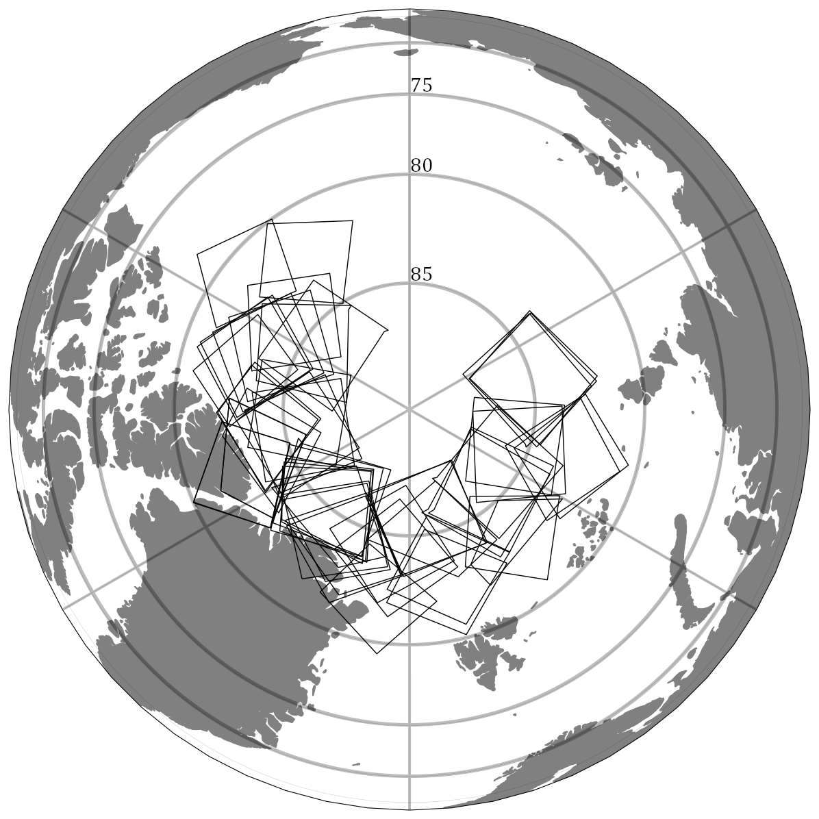
Figure 1 Location of all Sentinel-1 scenes from October or November (2018–2022) with near-coincident ICESat-2 coverage. These acquisitions are the main source of data for this study.

On the altimetry side, we are using ICESat-2's ATL-10 sea ice freeboard measurement. ICESat-2 is an optical laser altimeter that operates at a wavelength of 532 nm and is highly pulsed at 10 000 pulses per second. The resulting altimetry measurement is accurate to approximately 2 cm. Because the freeboard segments are dependent on the scattering conditions of the surface (a certain number of photons are collected per segment), the spacing of the ATL-10 product is variable and on the scale of tens of metres. At these intervals, segments of freeboard height and expected variance are retrieved. To have as many data points as possible, we use the three weak beams, as well as the three strong ones, giving us a maximum of six beams from which data can be used. The benefit of including the less accurate weak beams is investigated later in the paper. Due to atmospheric conditions and the requirement of nearby open leads, a freeboard measurement is not always available when the instrument is measuring.

The bulk data in the study consist of 59 Sentinel-1 EW scenes and all ICESat-2 ATL-10 freeboard data obtained within 24 h of the SAR acquisition over the same footprint. The specific SAR scenes are selected because there exists an ICESat-2 overflight that is near-coincident with the SAR measurement (the time difference is less than 10 min), and the ATL-10 freeboard tracks overlap with at least 300 pixels of the SAR scene, each of 100 × 100 m² size. The near-coincident flights are important for observing the correlations between the measurements and, later, for validation of the extrapolation results. October and November are selected for two reasons: firstly, there exist comparatively many near-coincident acquisitions in this time period. This is likely due to atmospheric conditions, i.e. fewer clouds, as ICESat-2's laser at 532 nm does not penetrate these. Secondly, first-year ice is still quite young at this point and can therefore be more easily distinguished from older ice in both SAR and altimetry missions. As a result, the correlations between freeboard and backscatter are expected to be highest during this time of the Arctic sea ice cycle.

Setting the maximum time difference for a “near-coincident” measurement at 10 min and with pixel sizes of 100 m, significant decorrelation of both measurements can start to occur if the ice drifts faster than 50 m in 10 min (equating to 300 m h⁻¹). Such high drift speeds are reached occasionally, but this constraint to 10 min is sufficient to make sure the vast majority of data points are still valuable. The data are matched using the geocoding of both products, and no ice drift correction is applied. For Sentinel-1, the geolocation uncertainties reported by Schubert et al. (2017) are around 5 m over land, which we can use as a baseline error. Additionally, the geoid model used for the ground range projection will have an error relative to the real sea surface height, which should be of a similar scale as the local sea surface height anomaly. Skourup et al. (2017) investigated the model and observational differences and found differences in the central Arctic of up to 0.5 m. Thus, we can assume that the Sentinel-1 geocoding error is generally below 10 m. The geolocation errors of ICESat-2 are reported to be around 2.5 to 4.4 m by Luthcke et al. (2021). As the pixel sizes of 100 m are significantly larger than the uncertainties of the geocoding, we can obtain meaningful overlap between the SAR and freeboard products at this scale.

All ICESat-2 ATL-10 segments in one Sentinel-1 pixel are considered equally: to obtain a local freeboard, the mean of all freeboard segment heights from ATL-10 pertaining to a pixel is taken. For roughness, we investigate two different considerations that describe different roughness correlation lengths (scales). The ATL-10 product gives an expected variance for each freeboard segment, determined by local photon statistics, and, thus, is approximately at the metre scale. For the first roughness observation, all freeboard segments' respective variances are summed, and from the square root of their mean, a final standard deviation for each pixel is obtained, giving a roughness at approximately the metre scale. Alternatively, a larger-scale roughness can be obtained by calculating the standard deviation of all ATL-10 freeboard segment heights within one 100 m × 100 m SAR pixel. The correlation length or scale of this roughness measure is equivalent to the spacing of the segments, i.e. on the order of tens of metres. Both of these roughness measures use the variance of freeboard heights as a proxy for the roughness of the ice surface.

Correlations

We will first investigate the statistical connections of the altimetry and SAR data. In this case, we are mainly interested in the correlations of these variables as this will be of importance for the extrapolation measures described later.

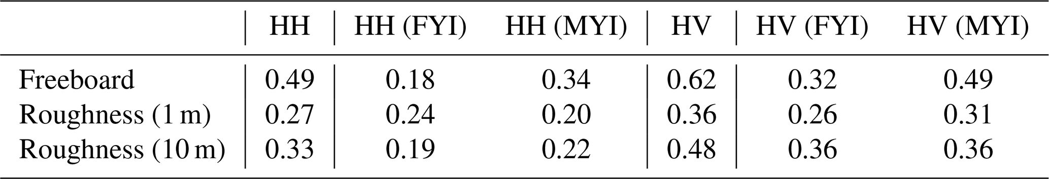
Heatmaps of both freeboard and roughness from all 597 565 data points are plotted in Fig. 2, along with the respective Spearman correlations. We use Spearman correlations here as we do not expect the values to be correlated linearly, but we are interested in how accurately we could construct a monotonic mapping from one to the other – which is exactly what the Spearman correlation coefficient captures. In Table 1, the Spearman correlation coefficients are listed. The split into multiyear (MYI) and first-year (FYI) ice is performed for 51 of these scenes (with 392 364 data points), which admitted a clearly bimodal freeboard distribution, allowing us to differentiate between the two ice types via thresholding of the freeboard. The other eight scenes did not show such a split distribution and thus were not considered.

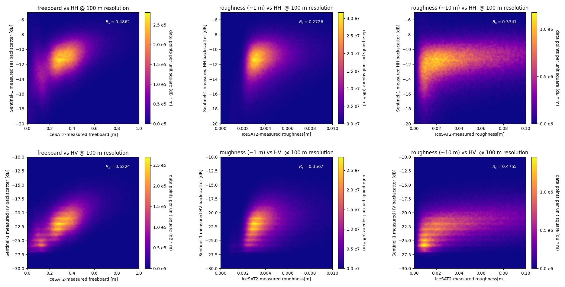
Figure 2 Two-dimensional histograms of ICESat-2 freeboard and roughness versus Sentinel-1 HH and HV backscatter measurements and the respective Spearman correlation coefficients. Brighter colours correspond to higher data density, whilst darker, blueish colours correspond to lower density. Some banding effects are visible in the HV channel.

There are three main studies from the Canadian Arctic Archipelago we can compare these results with, all of which focus on fast ice. Cafarella et al. (2019) investigated the statistical relationship of high-resolution C- and L-band SAR data (resolutions of ≈ 10 and 3 m, respectively) with airborne lidar-derived sea ice roughness (resolution = 1.2 m) over first-year ice. From two scenes acquired in the late-winter season (March, April), they found a high correlation (Pearson's R) of 0.86 for high incidence angles (46°) and a low correlation of 0.30 for low incidence angles for the HH backscatter and roughness. The correlation of the HV backscatter and roughness was found to be more similar across the two scenes, around 0.81 for high incidence angles and 0.68 for low incidence angles. Segal et al. (2020) observed the correlations of lidar-derived roughness, a roughness proxy from the MISR optical satellite and Sentinel-1 C-band SAR over first-year and multiyear ice in late winter (April). The roughness was derived from 1 m resolution lidar data, and the grid cells were 1.2 km × 0.4 km large. They found a high correlation (Pearson's) for roughness and HH backscatter at 0.74 across their whole dataset, with 0.76 on only first-year ice and 0.12 on only multiyear ice. Recently, Macdonald et al. (2024) published a study comparing SAR and altimetry measurements for three ICESat-2 overflights in the Canadian Arctic Archipelago in March. It is also worth noting that they computed roughnesses from the University of Maryland super-sampled ICESat-2 product, described in Duncan and Farrell (2022) and Farrell et al. (2020). As the source for SAR data, they used the Radarsat Constellation Mission (RCM) in a low-noise mode unique to the instrument and found (Spearman) correlations for first-year ice roughness and SAR backscatter of 0.42 for the HV channel and 0.31 for the HH channel. The correlations with multiyear sea ice height and backscatter were 0.49 in the HV channel and 0.41 in the HH channel. They also demonstrated an accurate roughness retrieval at the 800 m scale. The differences of between these previous studies and ours are the spatial scales, seasons, and location. While these previous studies were looking at a more regional scale, we use satellite overflights from more diverse Arctic regions. However, our roughness measures are not as fine scale or as accurate as the airborne lidar data or the University of Maryland ICESat-2 product. Additionally, we are focusing on the early-winter season rather than the late-winter season.

The freeboard correlations with the HV channel across our entire dataset are remarkably strong at 0.62. The correlation for MYI and the HV channel is the same as in the Macdonald et al. (2024) study at 0.49. However, the correlations with the roughness are weaker, especially in the HV channel, than in all previous studies. Causes for this could be the ice development, the difference in ice seasons, or the roughness measures used. Comparably low correlations were also found in Kortum et al. (2024) for sea ice roughness at length scales of 0.5 m with the HH and VV channels of X-band SAR. The correlations for freeboard across the entire dataset (R = 0.62) might be slightly stronger in this study compared to the Macdonald et al. (2024) study because of the rescaling to 100 m × 100 m, which should lead to an increase in correlations as quasi-random speckle effects average out. Additionally, the study area and time might be a cause for this, with both very thin first-year ice and the oldest, thickest perennial ice being captured within this study's dataset. This should also lead to an increase in correlation.

Table 1 Spearman correlation coefficients of ICESat-2 and Sentinel-1 measurements. The correlations for HH and HV are calculated from all 59 available flights. Of these, 51 admitted a bimodal freeboard distribution, allowing the separation of first-year ice (FYI) and multiyear ice (MYI).

3 Methods

3.1 Algorithm structure

The structure of the proposed freeboard extrapolation method using SAR backscatter is as follows.

1. For the SAR scene to be used as the basis for the extrapolation, all ATL-10 measurements within the last 24 h are retrieved.

2. A mapping from the HV SAR data to the non-coincident ATL-10 freeboard in the area is constructed via the cumulative distribution functions of the HV SAR measurement and the altimeter freeboard product.

3. The mapping is applied to the HV channel of the entire scene from step 1.

This extrapolation using the cumulative distribution functions relies entirely on the correlations of sea ice ageing processes and its freeboard, illustrated in Fig. 3. As young ice freezes up, a brine expulsion on top of the ice leads to a wet and saline surface and possibly wetted snow, as investigated by, for example, Drinkwater and Crocker (1988). This lossy material is quite absorbent, and backscatter is typically quite low, especially for double bounces required for HV returns. Whatever backscatter is measured probably originates from surface roughness features, which also increase freeboard. As the ice gets older and desalinates (Cox and Weeks, 1974), the bulk ice becomes less opaque to the radar waves, thus increasing the volume scattering from bubbles and empty brine channels. In turn, the HV signal becomes stronger. Finally, large topographical features, such as ridges, can accommodate double-bounce backscatter returns and can again increase the HV backscatter return. It is important to note that there is no direct physical connection between the backscatter and ice freeboard; i.e. there is no physical reason why a ridge 1.5 m high should have a stronger HV backscatter response than one only 1 m high, and this is therefore the strongest limitation of this approach. However, we propose that, in the vicinity of a measured freeboard distribution from ICESat-2, the backscatter is a reasonable predictor of relative freeboard heights and can therefore be used to extrapolate the freeboard measurements. This is possible because, in most cases, the freeboard distribution does not change drastically on a 100 km scale or within 24 h. Of course, using coincident flights rather than those within 24 h would yield better extrapolation results. However, these cases are extremely rare, and the coverage of such a product would be extremely sparse.

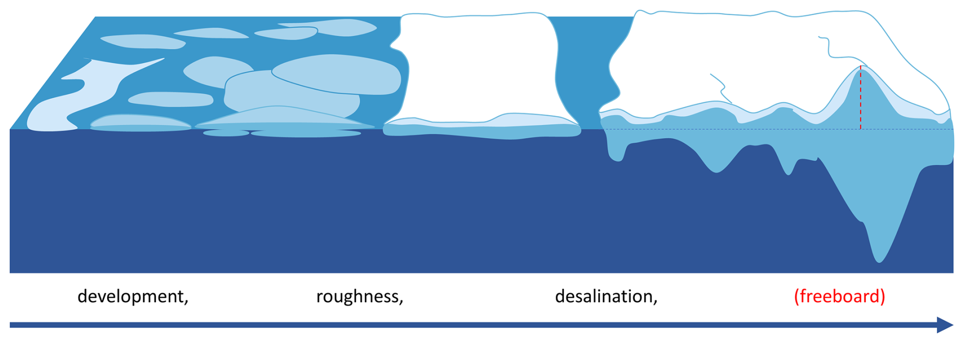
Figure 3 Illustration of the connection between freeboard and ice development responsible for the increase in HV backscatter (mainly desalination and surface roughness increase).

3.2 Cumulative distribution function (CDF) mapping

To create the mapping from Sentinel-1 backscatter to ICESat-2 freeboard using the cumulative distribution functions (CDFs), all ATL-10 data from the last 24 h within the footprint of the SAR scene are collected. They are resampled to match the 100 m pixel spacing from SAR. For our scenes, the resampling factor was approximately 10, which is used in the following. Their cumulative distribution function CDF_fb is formed from all measurements taken. For the CDF of the HV channel CDF_HV, all pixels within 1000 m of an ICESat-2 track are considered. Because the ice has drifted in between the measurements, it is not the same exact ice that forms both CDFs. However, restriction to the approximate area ensures that the distribution of the underlying ice is similar. The constructed CDF map is illustrated in Fig. 4 and can be expressed as

$$\begin{array}{}\text{(1)}& \begin{array}{l}\mathrm{\Phi }:\left\{{\mathit{\sigma }}_{\mathrm{HV}}\right\}\mapsto \left\{fb\right\},\\ \mathrm{\Phi }\left({\mathit{\sigma }}_{\mathrm{HV}}\right)=\left({\text{CDF}}_{fb}^{-\mathrm{1}}\circ {\text{CDF}}_{\mathrm{HV}}\right)\left({\mathit{\sigma }}_{\mathrm{HV}}\right).\end{array}\end{array}$$

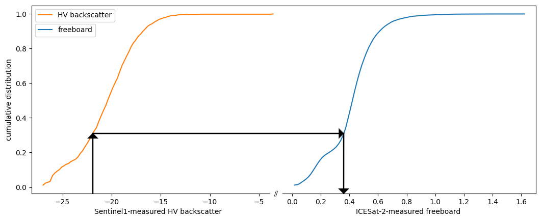
Figure 4 Visualisation of the mapping constructed from the cumulative distribution functions of freeboard and HV backscatter. The black path illustrates a mapping from an HV backscatter value to a freeboard value.

With this mapping constructed, pixels can be mapped from HV backscatter to freeboard for the entirety of the Sentinel-1 acquisition. It is worth noting that the Spearman correlation coefficient is invariant under such a monotonic transformation. Thus, all of the improvement between the Spearman correlations of the predicted freeboard and the measured freeboard in contrast to the HV backscatter and the measured freeboard comes from the different CDF mappings for each scene.

3.3 Validation

To validate the results of the method, the procedure described above is performed for all 59 SAR scenes that additionally have a coincident ICESat-2 overflight. To form the cumulative distribution function CDF_fb for the freeboard, all ATL-10 data within 24 h of the SAR acquisition are used, except for the validation flight within 10 min. Then the extrapolated freeboard is compared with the near-coincident validation overflight over the same scene. This ensures that the constructed mapping and extrapolated results are entirely independent of the validation data. Therefore, the validation results are representative of the algorithm performance in ice conditions in October and November. Validating with coincident ICESat-2 instead of helicopter-borne measurements such as those collected during MOSAiC (Nicolaus et al., 2022) or Operation Ice Bridge (MacGregor et al., 2021) ensures that errors arising from the difference in measurement techniques do not need to be accounted for.

4 Results

Figure 5 shows the central results of the predicted algorithm. At 100 m resolution, a Pearson correlation of 0.68 between the measured and extrapolated freeboard shows that the relationship of HV backscatter and freeboard can be used to make meaningful extrapolation possible. At just above 10 cm, however, the errors are still significantly greater than the uncertainties of the underlying ATL-10 product. Additionally, judging by the heatmap in Fig. 5, at 100 m resolution, this technique enables the separation of ice into approximate classes such as first-year or multiyear ice and the detection of ridges. As the resolution is reduced, the retrieval method becomes increasingly accurate, as is illustrated by the narrowing of the heatmap. At 400 m resolution, with a Pearson correlation R_p = 0.82 and errors of 6 cm, the retrieval method shows promising results that can unlock comprehensive freeboard surveys of the Arctic in two dimensions.

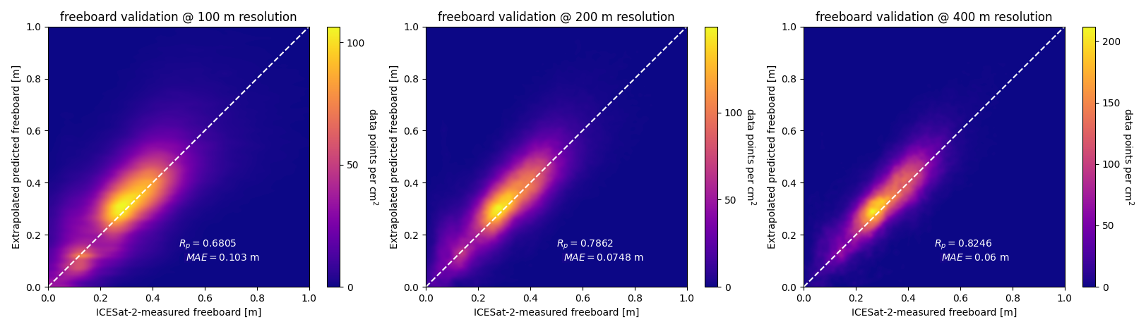
Figure 5 Results at different spatial resolutions (100, 200, 400 m) of the extrapolated freeboard data for all 59 scenes (597 565) data points, with Pearson correlation coefficients R_p and mean absolute errors (MAEs) shown in the figures. Brighter areas indicate a higher density.

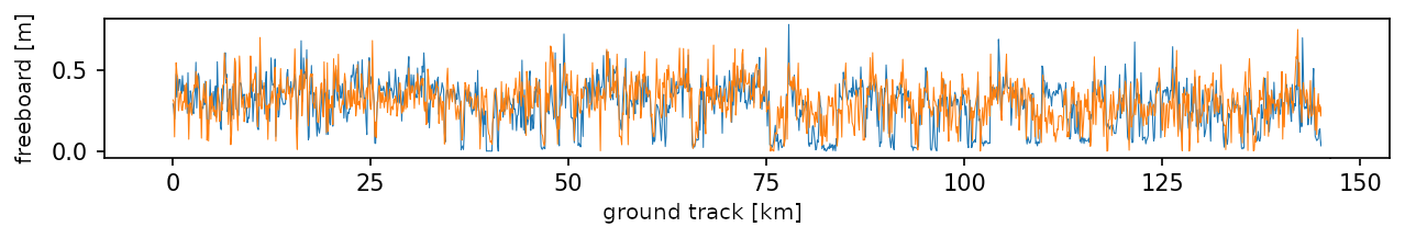
An example scene is shown in Fig. 6, where, qualitatively, the extrapolated freeboard aligns well with the overlaid ATL-10 measurements. The bottom track is shown in more detail in Fig. 7, where it becomes clear that, in most cases, the characteristics are captured well (R_Pearson = 0.67), but the exact height (especially for ridged areas) cannot be accurately approximated (RMSE = 0.08). Occasionally, some younger ice areas are shown to be significantly thinner than assumed from the extrapolation. These areas have also posed problems in sea ice classification algorithms in the past, for example, as described in Guo et al. (2023).

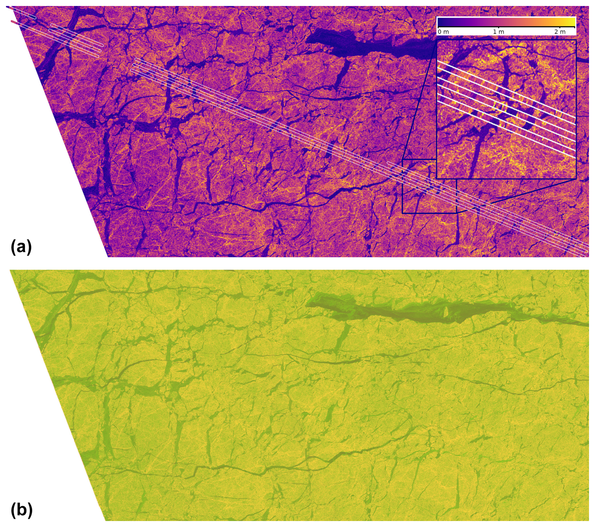
Figure 6 Example scene from 29 November 2021 with both the extrapolated freeboard at 100 m resolution and overlaid ICESat-2 ATL-10 data in panel (a). The ATL-10 data were thickened artificially (using nearest-neighbour extrapolation) to allow easier visualisation and are shown within the white contour. The three visible tracks are made up of one strong and one weak beam each. Panel (b) shows the SAR image in false colour. The composition (HV, HH, HV–HH) is chosen for the respective (R, G, B) channels.

Figure 7 Track of southernmost (bottom) beam from Fig. 6 with measured (ICESat-2, blue) and extrapolated (Sentinel-1, orange) freeboard values at 100 m spacing.

5 Error analysis

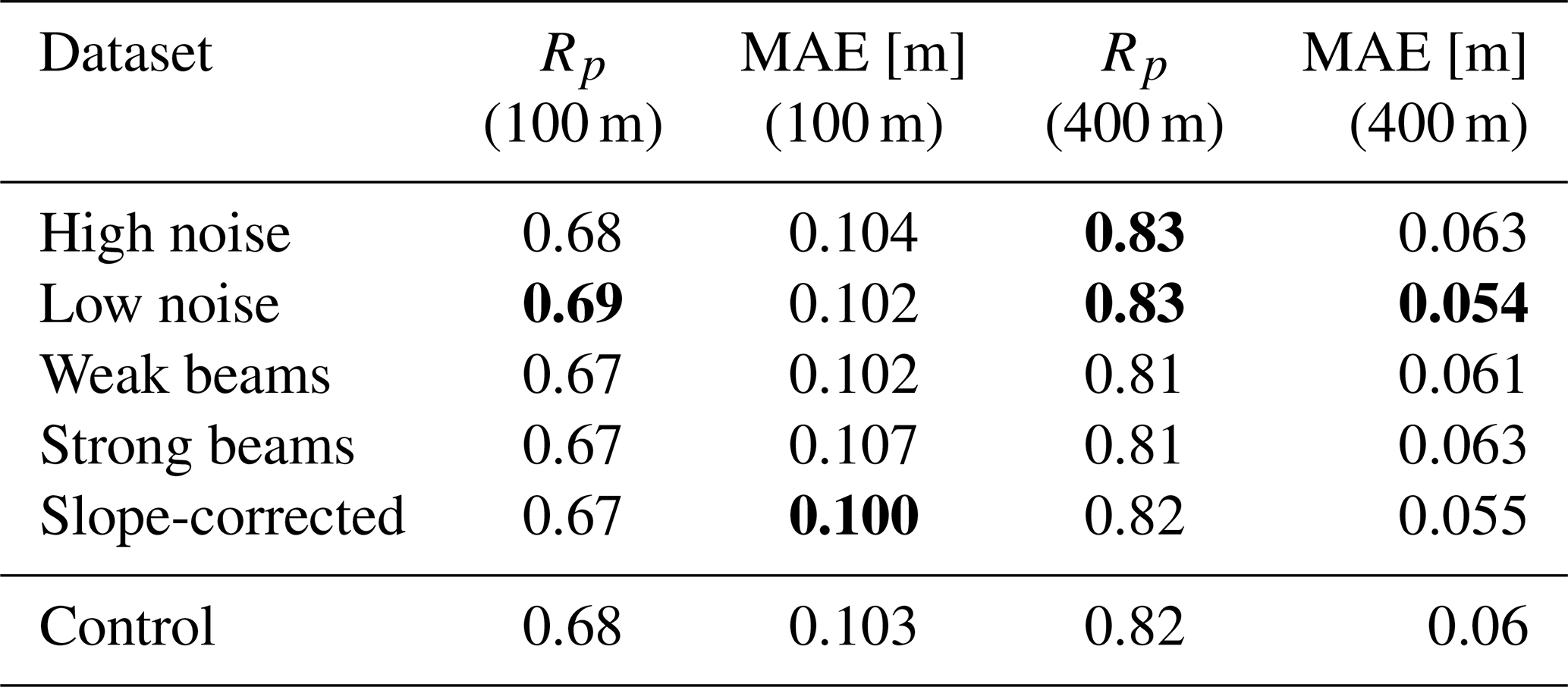
The approach detailed in this paper is heavily based on the statistical relationship between SAR HV backscatter and freeboard as measured by ICESat-2. Whilst we suspect the limitations of such a purely statistical relationship to be the greatest source of error for the extrapolation, we can measure the effect of various other contributions to the error directly. In this section, we investigate the influence of thermal noise, incidence angle effects, and strong and weak ICESat-2 beam selection on the accuracy of the final product. To do so, we split the dataset in a variety of ways. The combined results are presented in Table 2.

To measure the influence of thermal noise on the freeboard product, we split the Sentinel-1 scenes into two disjoint subsets according to the height of the noise floor. As a divisive criterion, we use −30 dB as the limit of the noise floor in the low-noise dataset. All data where the noise floor is higher than −30 dB are placed in the high-noise dataset. We then execute our algorithm exactly as before and compare the two datasets.

The incidence angle effect of sea ice for the HV channel is not well investigated in contrast to the effect on HH backscatter. In the study of Aldenhoff et al. (2020), the slopes are found to be roughly half as steep in the HV channel as in the HH channel. Kortum et al. (2023) also found weaker HV slopes in their investigation. Despite the effect being smaller, it still influences the brightness values and, therefore, the extrapolation of freeboard. To measure the effect of an incidence angle mitigation strategy on the freeboard extrapolation, we use a Gaussian clustering approach by Cristea et al. (2020). Thus, we obtain HV backscatter versus incidence angle slopes for every pixel in the scene and then use these to correct the entire image to a 30° incidence angle. We can then compare the accuracy of the freeboard extrapolation with and without the incidence angle correction.

Finally, we investigate the inclusion of weak beams of the freeboard measurement by constructing two additional datasets with only weak and only strong beams and comparing with the original one which included both.

From the results in Table 2 we can infer the following:

1. Restricting to areas of low SAR backscatter noise improves the correlation of extrapolated and measured freeboard slightly. In addition, the errors are lower in the low-noise areas (noise floor lower than 30 dB) by ≈ 14 %. However, such a correction would significantly reduce the coverage of obtained extrapolated data.

2. Restricting to weak or strong beams makes only a small difference. Including both gives the best results.

3. Slope correction improves or matches the results of the control dataset for the investigated measures, and the amount of extrapolated data is not negatively affected.

Table 2 Investigating the influences of noise, weak or strong beams, and SAR incidence angle on the freeboard extrapolation method through splitting the dataset along various criteria. Results are Pearson's R (R_p) and the mean absolute error (MAE) between extrapolated and measured (coincident) freeboard. We show results for the 100 m product and the 400 m resampling. The control dataset uses the results described in the Methods section, with both strong and weak beams and all incidence angles included but no incidence angle correction carried out. Best-in-category results are highlighted in bold font.

6 Comparison with upward-looking-sonar data

To gain additional insight into the extrapolation performance and to demonstrate the usefulness of such an approach, we compare the extrapolated freeboard product to upward-looking-sonar data at mooring B (78° N, 150° W), acquired by Krishfield et al. (2023). The upward-looking sonar measures the ice draft from below. In theory, having both measurements – the freeboard from above and the draft from below – available allows us to characterise the ice (and snow) thickness. The advantage of the upward-looking sonar is that it is constantly acquiring, and, therefore, we can evaluate all scenes that capture the location of the sensor for comparison. We conducted this comparison for the entirety of November 2022 using 29 SAR scenes. The results are presented in Fig. 8.

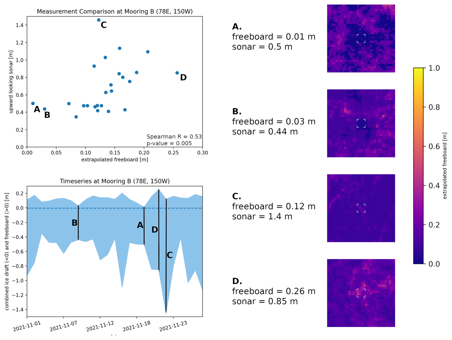
Figure 8 Comparison of extrapolated freeboard and upward-looking-sonar data. Four statistical outliers (A–D) are investigated in more detail, with freeboard extrapolation in the area shown on the right. The 16 central pixels used for comparison are indicated by the white brackets.

The greatest challenge in bringing these two measurements together is the difference in scales. We are working with a 100–400 m freeboard product, but the footprint of the sonar is only approximately 2 m. To enable sensible comparison, we use 10 min of sonar data around the acquisition time of the satellite and the 400 m SAR product. As a result, we have a 2 m thick line sampled by the sonar (with the length depending on the drift speed) being compared with 400 m × 400 m area of extrapolated freeboard. This means that the distribution of the ice sampled in the freeboard maps should overlap with the sonar coverage, but the area sampled by the satellite is much larger. This is a circumstance we cannot mitigate further. The scatterplot in the top left of Fig. 8 shows that there exists a clear statistical correlation between freeboard and ice draft – as one would expect. It also shows that the relationship breaks down below around 0.5 m of ice draft. For such relatively young ice, the freeboard values are probably not accurate. We investigate this further in two outlier cases, A and B. From the freeboard map, it becomes obvious that the dynamic range of the HV measurement is not able to capture the subtleties of the backscatter response as we are too close to the noise floor. This is apparent from the strong edges of the low ice areas in the freeboard maps. Another outlier, C, shows a high ice draft but medium freeboard. The freeboard map reveals that we are in an area of rather young ice but with signs of ridging, as can be seen from the linear features with higher freeboard. In fact, such a ridge area is right in the measured area. Therefore, we suspect that the sonar sampled a large part of that ridge's keel, while the contribution is only small in SAR. In other words, the difference in sampling scales or footprint sizes is the reason for this strong disagreement. In the final outlier, D, we have the opposite scenario, where the freeboard is large, yet the ice draft is not. The freeboard map shows a highly diverse ice area. Again, it is likely that the two distributions sampled by the two measurements are quite different due to their differences in terms of scale and the limited overlap.

This brief excursion showed how freeboard extrapolation enables the comparison and combination of altimeter-derived freeboards with additional measurements. It also revealed that thin-ice areas below 0.5 m ice thickness with low HV backscatter cannot be accurately extrapolated with the proposed CDF-based mapping. As expected, sampling scales are a considerable challenge in combining upward-looking-sonar data with satellite sea ice measurements.

7 Discussion

The correlations between the SAR backscatter and altimetry freeboard and roughness data found in this study join those observed in previous studies by Cafarella et al. (2019), Segal et al. (2020), and Macdonald et al. (2024) to form a more complete picture of the variability and correlations of SAR and topographic ice properties. As mentioned earlier, the study area and time are probably the main reason for the differences in observed correlations. The data studied here suggest that relating roughness and backscatter is more difficult in the early-winter season than in the late-winter season investigated by previous studies. However, correlations with freeboard are still significant, which reinforces the notion that they can be successfully related to one another.

This study is the first time these correlations between satellite laser altimeter freeboard and SAR backscatter were observed for drifting sea ice across a large area in the Arctic. The correlations of 0.68 (100 m scale) to 0.82 (400 m scale) of freeboard and the SAR HV channel are remarkably high considering the fact that there is no direct physical connection between backscatter and freeboard.

The results reveal that the proposed algorithm enables meaningful extrapolation of ice freeboard as measured by ICESat-2, capturing key features and revealing the spatial variability of freeboard in two dimensions at 100 to 400 m resolution and for the coverage of full 400 km Sentinel-1 scenes. The accuracy of the retrieval is difficult to judge in relation to other methods as no comparable products exist. The algorithm performs accurately enough to separate ice types and ridges at 100 m resolution, with errors of around 10 cm. At 400 m resolution, the method is even more accurate given an error of approximately 6 cm.

We also demonstrated a comparison with other sea ice measurements in the case of the upward-looking sonar (ULS), which is enabled by the extrapolation effort. The comparison of satellite ice freeboard and ULS ice draft reveals a reasonable correlation of 0.58 between the dataset and the fact that the correspondence breaks down below about 0.5 m ice thickness. However, the difference in terms of measurement scales limits the information that can be derived from such a combination. With additional effort, cases with two satellite acquisitions and largely homogenous drift could be found. In this case, the displacement between the two scenes can be derived, and the drift between points can be assumed to be a straight line. Then the overlap between two measurements would greatly increase, and, in part, the difference in terms of scales could be mitigated.

As previously mentioned, the main source of the remaining retrieval uncertainties is the absence of a physical connection between topography and SAR backscatter, something that cannot be circumvented. Additional sources of error also exist. For example, the footprints of ICESat-2 do not cover the entire pixel they are being mapped to, meaning the ground truth we use for freeboard in every pixel is already contaminated by this undersampling. In addition to the existing uncertainty of the ATL-10 products, SAR noise and speckle effects also contribute to the error. Furthermore, the overlap of the validation overflights is limited by the accuracy of the georeferencing of the sensors. In the case of Sentinel-1, the GRD product uses an ellipsoid model, which can vary by up to tens of metres from the real ocean surface height.

Investigations into the incidence angle effect have shown that a brightness correction using slopes derived from a clustering method is a successful measure to mitigate the influence of incidence angle on backscatter and, thus, the extrapolation algorithm.

It was also shown in Table 2 that restricting to weak beams yielded slightly better results than restricting to strong beams, which is counter-intuitive. The weak beam segments are derived from the same number of photons. As these take longer to accumulate for the weaker beams, the segments become longer. Keeping in mind that the strong extrapolations were evaluated against measurements from strong beams and vice versa for weak beams, we offer two possible explanations for this. Firstly, the beams are not always available (or unavailable) at the same time, and so it is possible that the correlation between freeboards and backscatter is stronger in the weak-beam dataset simply by chance. The other possibility is that the matching of the pixels via geolocation is not quite pixel perfect, and the longer weak segments align better as they smooth the validation measurements a little.

Overall, this purely statistical mapping is rather simple, given the complexity of the physical relationship between sea ice properties, such as freeboard, and the radar backscatter of a SAR sensor. However, we believe there is great merit in having such a simple and explainable method to advance scientific work in this field. For future work, it is very valuable to have such a baseline algorithm available to compare with or to use as a basis for more complex methods.

So far, the extrapolation has been limited to only a certain season in the year, i.e. October and/or November, where older and younger ice have significantly different freeboards, increasing the correlation with SAR backscatter. Expanding this approach to other seasons and the marginal ice zone will be more challenging. Part of the reason for this is that the amount of overlapping data at 10 min of time difference, needed to validate the results, is sparser in other months and non-existing inside the marginal ice zone.

We have validated the approach with independent, near-coincident ICESat-2 flights. Comparison with CryoSat-2 radar altimeter measurements would be the next logical step. Because of the different dominant scattering surface of that radar instrument, however, the freeboard measured by CryoSat-2 is different from that measured by ICESat-2, as shown in Fredensborg Hansen et al. (2024) using the Cryo2Ice data. Therefore, it is less useful as validation data. It would be very interesting to investigate the possibility of extrapolating CryoSat-2 and future CRISTAL measurements using the same method and comparing the results. Additionally, the new surface water and ocean topography (SWOT) altimeter allows for 2D freeboard retrieval that would be a great candidate for validation or extrapolation. Work by Kacimi et al. (2025) has shown good correlations with the ATL-10 freeboard used here. However, SWOT's coverage is restricted to 78° north–south, and, therefore, its use for sea ice applications is unfortunately limited, but a case study comparison might be possible.

Whilst we worked with extrapolating ICESat-2's ATL-10 product from NASA, other current or future altimetry products might also be able to be extrapolated with SAR. For example, the University of Maryland product by Farrell et al. (2020) and Duncan and Farrell (2022) mentioned earlier would be worth using instead of the ATL-10 data for the roughness approximation, as was done in Macdonald et al. (2024). As the main focus in this study was on freeboard, this was not considered.

The uses of a medium- to high-resolution freeboard product are manifold. The data can be used as a good proxy for sea ice thickness in terms of variability in two dimensions, something that has so far eluded consistent observation. Maritime stakeholders might also profit from these data, as well as weather and climate models, the former of which could be initialised with observations in near-real time. High-resolution digital twin Earth models, such as those currently in development by Hoffmann et al. (2023) at ECMWF, might benefit from these observations in particular due to their kilometre-scale grid spacing.

8 Conclusions

Our work as presented in this paper shows how ICESat-2-derived freeboard measurements can be meaningfully extrapolated with Sentinel-1 SAR measurements at resolutions of up to 100 m for the entire 400 km SAR scene with up to a 24 h time difference between SAR and altimetry acquisitions and a freeboard extrapolation error lower than 10 cm. This algorithm opens up an opportunity to monitor Arctic-wide sea ice freeboard in two dimensions, capturing its spatial variability at previously unattainable coverage and making an important step towards monitoring ice thickness. It has yet to be shown whether this approach can also work throughout all seasons and regions of the Arctic.