Interannual variability in air temperature and snow drives differences in ice formation and growth

Recent warming of northern high-latitude regions has raised critical concerns regarding the safety and reliability of frozen lakes for winter transportation and recreation. This issue is particularly significant in Canada's Northwest Territories (NWT), where seasonally constructed roads over lakes, rivers, and land (winter roads) span thousands of kilometers and act as vital links to isolated communities and resource development projects. Current climate change and weather variability are altering the evolution of lake ice, challenging predictions of freeze-up, ice growth, and ice decay. The accurate simulation of ice evolution is imperative for safe and efficient planning, operation, and maintenance of winter roads under a changing climate and heightened weather variability. This is particularly significant in the early winter period when ice road planning and design are undertaken. Here, we investigate the effects of weather variability on ice formation, growth, and evolution in a small lake near Yellowknife, NWT, Canada. High-resolution measurements of air, snow, ice, and water temperatures were collected continuously from a floating research station between October and December in 2021, 2022, and 2023 and variability in ice evolution and weather examined. Combinations of above- and below-average snowfall and winter air temperatures resulted in variability of up to 17 d in freeze-up dates (FUDs) and 8 d in freeze-up durations. By the end of December, ice thicknesses (h_i) varied up to 12 cm, while the duration between the FUD and h_i=30 cm varied up to 10 d. Ice thickness was effectively simulated (RMSE=1.11–2.33 cm) using empirical relationships developed using cumulative freezing degree days (CFDDs) and seasonally cumulative snowfall (S_T), while snow ice thicknesses was simulated (RMSE=0.83–1.21 cm) using CFDD and daily snowfall. Developed relationships between air temperatures, snow, and ice thicknesses can be used for predicting the minimum ice thicknesses required for commencing ice road planning and construction management under increasingly variable climatic conditions.

1 Background

Ice covers act as critical infrastructure for northern regions by means of seasonally constructed roads over lakes, rivers, and land (winter roads). Winter roads allow for the cost-effective transportation of vital goods and services to isolated communities (Barrette et al., 2022) and remote mining projects (Hayley and Proskin, 2008). Winter roads support critical resource development projects across Canada and contribute substantially to the Canadian economy (Prowse et al., 2009). Further, the presence of snow and ice over lakes inherently affects the ecological and geochemical processes of lakes (e.g., Huang et al., 2021; Song et al., 2019) and is used as indicators of climate change (Kheyrollah Pour et al., 2014a, b; Palecki and Barry, 1986; Skinner, 1993; Attiah et al., 2023).

Phenological changes in lake ice cover have been explored across many northern high-latitude regions and strongly relate to weather conditions (Huang et al., 2019; Latifovic and Pouliot, 2007; Leppäranta et al., 2017). There is coherence amongst most published literature that lakes across the Northern Hemisphere are experiencing earlier break-up dates (BUDs), with some exceptions depending on the time periods analyzed, significance levels attributed to trends, and specific regions. Trends of earlier BUDs have been observed in Canada (1961–1990; Duguay et al., 2006), Sweden (1870–2010; Hallerbäck et al., 2022; L'Abée-Lund et al., 2021), Poland (1961–2010; Choiński et al., 2015), Lake Baikal (1869–1996; Todd and Mackay, 2003), and the Laurentian Great Lakes Region (1975–2004; Jensen et al., 2007). Meta-analyses conducted by Newton and Mullan (2021) and studies derived from the Global Lake and River Ice Phenology (GLRIP) Dataset produced by Benson et al. (2000), spread mostly across North America and northern Europe, show similar results.

Trends in freeze-up dates (FUDs) have shown much greater spatial variability, as ice formation depends strongly on local topography, lake morphology, and lake heat storage (Leppäranta, 2015). Regional trends in FUDs are often masked, under-represented, or not available, particularly in meta-analyses where the majority of a lake may show later FUDs (e.g., Sharma et al., 2021; Basu et al., 2024). In meta-analyses, definitions used for delineating FUDs and methods of observation of ice formation vary in space and with time, creating a challenge for drawing accurate conclusions (Catchpole and Moodie, 1974; Wynne, 2000), as does the length of the available data record (Benson et al., 2012, supplementary material; Sharma et al., 2021, supplementary material). Notable examples of lakes with earlier observed trends in FUDs include Finnish Lapland (1930s–1960s; Korhonen, 2006), Xinjiang (2001–2018; Cai et al., 2020), eastern Canada (1961–1990), the Great Lakes–St. Lawrence regions (1951–1980) (Duguay et al., 2006), Kazakhstan and Tajikistan (2002–2022; Hou et al., 2022), Latvia (1945–2002; Apsîte et al., 2014), Poland (1960–1989; Girjatowicz et al., 2022), Sweden (1913–2014; Hallerbäck et al., 2022), and the Qinghai–Tibetan Plateau (2002–2021; Sun et al., 2023; 2000–2011; Yao et al., 2016). Trends of earlier FUDs in the last 30 years are of particular interest as they largely contrast the findings presented in Newton and Mullan (2021) and Sharma et al. (2021), who argue synchronicity in later freeze-up dates.

To better understand interactions between weather and climate and ice formation and growth, high-frequency in situ observations of interactions between air, snow, ice, and water should be monitored. Conventionally, high-frequency manual measurements of ice thicknesses and snow depths are constrained by finances, labor, site access, and ice safety and often result in discontinuous datasets. Numerical modelling provides a continuous alternative to frequent in situ measurements; however, models may be computationally constrained and still require frequent in situ observations for appropriate calibration. The use of a floating research station addresses these limitations through offering a cost-effective method to measure ice thicknesses and snow depths at high frequencies, without safety constraints, and can provide the necessary in situ data to calibrate numerical models. This approach facilitates the development of physics-based and/or empirically derived understandings of ice–atmosphere interactions for integration in lake models and global upscaling. In particular, improved understanding of ice formation and growth in early winter (October–December) can be essential for the effective and safe scheduling of the operating windows, choice of construction equipment, and the hazard control plans for ice road design.

In this study, we investigate the effects of interannual and seasonal variability on ice formation and growth in a small subarctic lake in the Northwest Territories (NWT), Canada. We compare weather variability in three early-winter periods (September–December 2021, 2022, and 2023) against the historical climate record (1942–2023) to understand driving forces in variability in freeze-up, ice onset, and ice growth. Empirical relationships between snow ice, total ice, and snowfall are developed using the acquired data for practical consideration for ice road design processes.

2 Study area and floating research station

This study aims to relate weather variability with ice formation and growth in Landing Lake, a small subarctic lake ∼11 km north of Yellowknife, NWT, Canada (Fig. 1). Landing Lake has a surface area of 1.07 km² and mean and maximum depths of 1.77 and 4.28 m (Rafat et al., 2023). The lake drains a relatively large catchment of 135 km² (Spence and Hedstrom, 2018) and is part of the larger Baker Creek Research Watershed (BCRW). BCRW is a well-studied, 155 km² Canadian Shield subarctic watershed consisting of 349 small lakes (Spence and Hedstrom, 2018). The watershed is drained by Baker Creek, which flows into Great Slave Lake. The basin is located within a region of discontinuous permafrost and large changes in topography, vegetation, hydrology, and surficial geology (Morse and Wolfe, 2017; Phillips et al., 2011). Land coverage in the BCRW is split between exposed bedrock (∼40 %), water (∼22.6 %), forested hillslopes (∼21.5 %), and wetlands or peatlands (∼15.9 %) (Spence and Hedstrom, 2018).

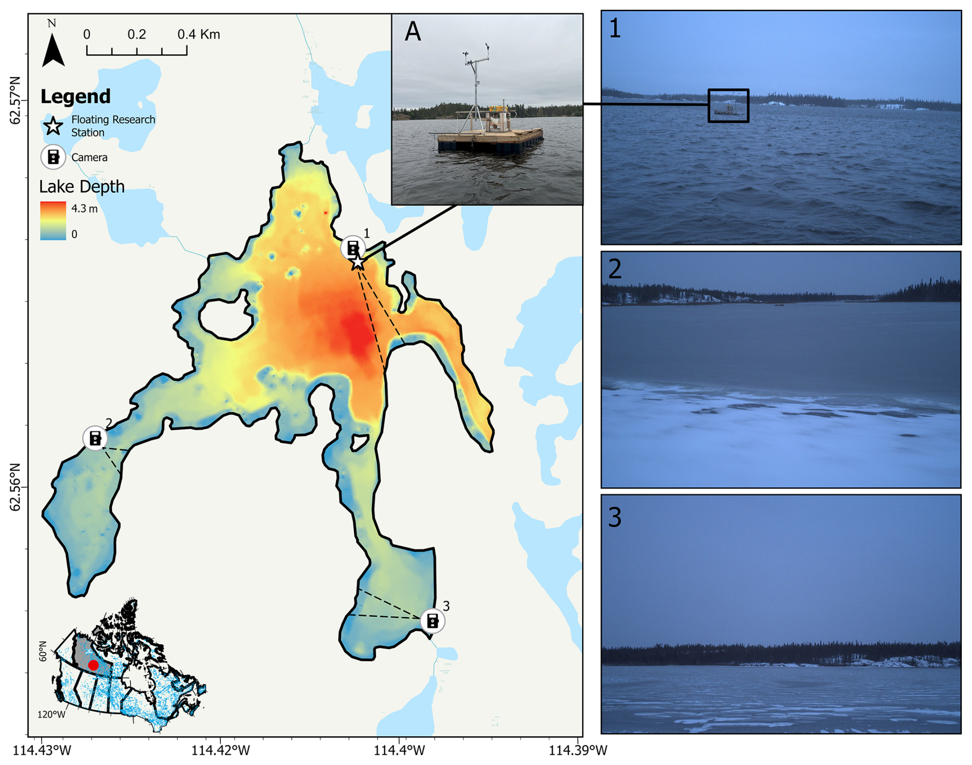
Figure 1 Site map of Landing Lake, Northwest Territories, including photographs of the floating research station (FRS) and perspectives from trail cameras (1, 2, and 3). Photographs 1, 2, and 3 were taken on 23 October 2023 at 09:00 LT and present three perspectives of the lake during the freezing process.

Yellowknife has a subarctic continental climate (Köppen Dfc). Annual precipitation is 288.6 mm, with 157.6 cm of snowfall. Snow begins to accumulate in October and melts in April (Spence and Hedstrom, 2018). Climate normal (1981–2010) mean annual air temperatures are −4.3 °C (Environment Canada, 2025). Summers are cool with peak mean daily air temperatures in July of 17.0 °C. Winters are cold and dry. Below-freezing air temperatures persist for >6 months of the year, with January mean daily air temperatures of −25.6 °C.

In October 2022, a floating research station (FRS) was built and deployed in Landing Lake to monitor the annual evolution of ice and snow. The FRS was anchored at a depth of 3.00 m (62.56° N, 114.40° W) and consisted of a 2.44 m×2.44 m floating structure. The FRS was instrumented with a snow and ice mass balance apparatus (SIMBA) thermistor chain, two pressure transducers (one in the water, one in the air), 10 digital temperature sensors near the lake bed, a CTD sensor (YSI EXO2 Sonde), two photosynthetically active radiation (PAR) sensors in the water, and a weather station tripod (that measures wind speed and direction, air temperature, relative humidity, and incoming and outgoing shortwave radiation). PAR sensors were installed in the water column at heights of 0.85 and 1.27 m above the sediments. A larger meteorological station located 100 m east of the FRS on an island in Landing Lake provides supplemental measurements of turbulent and radiative heat fluxes (Spence and Hedstrom, 2018). Figure 2 presents a schematic of the FRS.

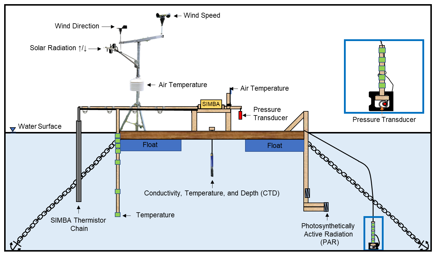
Figure 2 Instrumentation on board the floating research station (FRS), Landing Lake, Northwest Territories.

3 Methodology

3.1 Interface detection and manual observations

Air, snow, ice, and water interfaces were identified using SIMBA. SIMBA operated in two modes. Mode I took direct measurements of the ambient temperatures surrounding each sensor every 15 min. Mode II operated every 6 h. Over a 2 min heating cycle, Mode II applied a 64 mW constant and linear heat source to resistors housed beside each of the 145 sensors. The associated temperature rise at each resistor was recorded by adjacent temperature sensors every 30 s. Four additional measurements were taken in the proceeding 2 min to measure the cooling response at each resistor as the applied power was discontinued. Mode II provided a means of approximating the thermal conductivity of ice and snow, mimicking the transient hot-wire method for measuring thermal conductivity (Healy et al., 1976; ASTM International, 2022) and allowed for improved interface detection (Jackson et al., 2013). SIMBA has been widely used in monitoring sea ice (e.g., Koo et al., 2021; Lei et al., 2018) and, more recently, in river ice (Lynch et al., 2021) and lake ice evolution (Cheng et al., 2021; Rafat et al., 2023).

The position of the ice (or water) surface was identified by combining the information from Mode I and Mode II of SIMBA. The temperature rise after 2 min of gentle heating was lower in water compared to air, as water has a larger heat capacity. Likewise, the temperature rise in ice was lower compared to air, given the comparably large thermal conductivity and density of ice, thereby effectively transferring heat away from the source. Compared to one another, however, the temperature rise in water, ice, and slush is similar, normally ranging between 0.4 and 0.75 °C. Snow is excluded from this range as temperature rises in snow were significantly higher. Therefore, beginning at the top of the chain, the position of the water, ice, or slush surface would be the first sensor where the temperature rise after 2 min of heating would be between 0.4 and 0.75 °C. To delineate between water and ice, Mode I measurements at the identified location were analyzed. If the temperature (T) was $\le -\mathrm{0.5}$ °C, the surface was identified as ice; if T≥0.125 °C, the surface was water; and if $-\mathrm{0.5}\mathrm{°}\mathrm{C}<T<\mathrm{0.125}\mathrm{°}\mathrm{C}$, the surface was unfrozen slush.

The position of the air–snow interface was identified by selecting the location where the spatial derivative was a maximum, beginning from the top of the thermistor chain. Since snow is an effective insulator, vertical gradients in temperatures would present a distinct peak when transitioning from air to snow. To identify the position of the ice bottom, Mode I of SIMBA was used. For each measurement, the thermistor chain was searched between the bottom of the chain and the identified ice (or water) surface. The first sensor with $-\mathrm{0.5}\mathrm{°}\mathrm{C}\le T\le -\mathrm{0.0625}\mathrm{°}\mathrm{C}$ was selected to be positioned at the ice bottom, provided that the sensor immediately above this identified location also fell within the noted range to reduce uncertainty. The range was selected to account for the manufacturer-specified accuracies of the sensors and the minimum resolution of the thermistors of ±0.0625 °C. Ice thicknesses were calculated as the difference between the identified ice bottom and surfaces, while snow depths were calculated as the difference between the snow and ice surfaces. If the ice surface is identified at a position that is higher up the chain than its original position, snow ice has formed. Therefore, snow ice thicknesses could be calculated as the difference in these positions. Further details on interface detection and its validation in Landing Lake are presented in Rafat et al. (2023).

Manual and pre-FRS observations

No direct measurements of air, surface, or water temperatures were available prior to the first installation of SIMBA in Landing Lake on 6 December 2021. For determining the freeze-up date (FUD) and date of ice onset (IO), daytime values from the MODIS/Aqua Land Surface Temperature/Emissivity Daily L3 Global 1 km SIN grid product (MYD11A1) and Sentinel-2 optical imagery were utilized. FUDs measured in situ at the FRS in 2022 and 2023 were verified using the same approach for validation. Imagery was acquired from Sentinel Hub's EO browser (https://www.sentinel-hub.com/, last access: 4 April 2025). In this study, freeze-up duration is defined as the period between the first occurrence of ice (ice onset, IO) and the formation of a solid ice cover over the entire lake (FUD). Manual measurements of snow depth and ice thickness were taken between November and December 2021, 2022, and 2023 for comparison with the SIMBA measurements. Three trail cameras (RECONYX Hyperfire 2) were deployed along the shoreline of Landing Lake to capture the freeze-up process: one was installed in October 2022 (camera 1, Fig. 1), and two more cameras (cameras 2 and 3, Fig. 1) were installed in October 2023.

3.2 Air and snow parameters and frequency analysis

To assess the influence of weather variability on ice growth, air temperature and snowfall parameters between September and December 2021, 2022, and 2023 were compared with in situ measurements of ice and snow evolution. Several air temperature and snowfall parameters were selected in this study for achieving this objective. For air temperatures, daily mean air temperatures (T_M) measured from the Yellowknife Airport weather station, located 11 km south of Landing Lake, were chosen. T_M was averaged for each month between September and December and for the bulk September–December 4-month period. As a first-order approximation of ice growth potential, the cumulative freezing degree days (CFDDs) in each month and for the September–December period were calculated. CFDD is ubiquitously used for estimating ice growth using Stefan's equation. For evaluating interannual variability in snowfall, several parameters were selected, including the day on which the first snowfall occurred (S_ON), the cumulative snowfall (S_T), the peak hourly snowfall rate in a given day in each month (S_p), and the number of snowfall days (S_d). Snowfall was recorded at the Yellowknife Airport weather station using high-frequency measurements of freshly fallen snow collected either manually (prior to 2022) or using an SR50 ultrasonic ranging sensor. In this study, we define the timing of zero-degree isotherm as the first date when mean daily air temperatures fell and remained below freezing (0 °C) for 3 consecutive days.

The severity of a given snowfall parameter (S_T, S_ON, S_p, and S_d) was evaluated using a frequency analysis conducted on the entire observational data record from the Yellowknife Airport weather station (1942–2023). For a given parameter, the probability of exceedance (P_e) in any given year was determined using Eq. (1), where m is the rank of the data and n is the length of the data record (82 years). The return period (R_P) was determined using Eq. (2).

$$\begin{array}{}\text{(1)}& {\displaystyle }{P}_{\mathrm{e}}={\displaystyle \frac{m}{n+\mathrm{1}}}\text{(2)}& {\displaystyle }{R}_{\mathrm{P}}={\displaystyle \frac{\mathrm{1}}{P_{\mathrm{e}}}}\end{array}$$

A Log-Pearson Type III (LP3) distribution was fit to the ranked data. LP3 is a well-studied distribution commonly used in hydrological applications and has been extensively used in flood frequency analysis and forecasting (Bobée, 1975). The logarithm of each parameter Y was determined using Eq. (3a–c). The antilog of Y values is evaluated following Eq. (3c) for interpretability.

$$\begin{array}{}\text{(3a)}& {\displaystyle }K={\displaystyle \frac{\mathrm{2}}{G}}\left\{{\left(\left[z-{\displaystyle \frac{G}{\mathrm{6}}}\right]{\displaystyle \frac{G}{\mathrm{6}}}+\mathrm{1}\right)}^{\mathrm{3}}-\mathrm{1}\right\}\text{(3b)}& {\displaystyle }G={\displaystyle \frac{n}{(n-\mathrm{1})(n-\mathrm{2})}}\sum _{i=\mathrm{1}}^n{\left({\displaystyle \frac{\log \left(Y_{\mathrm{i}}\right)-\log \left(\stackrel{\mathrm{‾}}{Y_{\mathrm{i}}}\right)}{{\mathit{\sigma }}_l}}\right)}^{\mathrm{3}}\text{(3c)}& {\displaystyle }\text{Log}\left(Y\right)=\stackrel{\mathrm{‾}}{\log \left(Y\right)}+K{\mathit{\sigma }}_l,\end{array}$$

where G is the skewness coefficient, K is the frequency factor depending on the return period and skewness, n is the length of record, $\stackrel{\mathrm{‾}}{\log \left(Y\right)}$ and σ_l are the mean and standard deviation of the logarithm of snowfall totals for any given month over the entire data record, and z is taken as the standard normal deviate.

3.3 Heat storage

Freeze-up is directly related to the heat storage in a lake. Hence, it is necessary to estimate the heat storage in the water column of a lake to understand the ice freeze-up and growth process. The rate of change in heat storage (${\dot{E}}_{\mathrm{T}}$) in Landing Lake was estimated using measurements of temperature at each sensor along SIMBA's thermistor chain located on the FRS (Eq. 4). h_i,btm represents the ice bottom (or water surface if no ice has formed), z_T is the lowest measurement points along the thermistor chain, ρ_w=1000 kg m⁻³ and c_p,w=4186 $\mathrm{J}{\mathrm{Kg}}^{-\mathrm{1}}\mathrm{°}{\mathrm{C}}^{-\mathrm{1}}$ represent the density and heat capacity of freshwater (respectively), and T_w represents the SIMBA-measured water temperature. ${\dot{E}}_{\mathrm{T}}$ is presented in units W m⁻².

$$\begin{array}{}\text{(4)}& {\dot{E}}_{\mathrm{T}}={\displaystyle \frac{\partial }{\partial t}}\underset{h_{\text{i,btm}}}{\overset{z_{\mathrm{T}}}{\int }}{\mathit{\rho }}_{\mathrm{w}}{c}_{\text{p,w}}{T}_{\mathrm{w}}\left(z\right)\mathrm{d}z\end{array}$$

4 Results

4.1 Variability in weather and climate

Mean daily air temperatures and cumulative snowfall between September and December 2021, 2022, and 2023 displayed large interannual variability and variability in reference to the climate normal and preceding 30-year periods (Fig. 3, Table 1). T_M in September, October, and November 2021–2023 was significantly greater than the 1981–2010 climate normal and 1992–2021 periods (Table 1). Both December 2021 and 2022 were colder than the climate normal and 1981–2010 periods by >3 °C, while December 2023 had anomalously high $T_{\mathrm{M}}=-\mathrm{13.6}$ °C, being ∼8 °C warmer on average than both reference periods. October 2021, 2022, and 2023 T_M had above-freezing temperature in contrast to both the climate normal and preceding 30-year record where T_M<0 °C (Table 1). The years 2021, 2022, and 2023 also showed notable variability in minimum (T_Min) and maximum (T_Max) daily air temperatures, particularly in October 2021 where T_Min>0 °C and T_Max were 3.3 and 3.9 °C greater than the climate normal and the preceding 30-year record, respectively. Despite interannual and long-term variability in T_Min and T_Max, the range between T_Max and T_Min remained similar in reference to the climate normal and preceding 30-year periods.

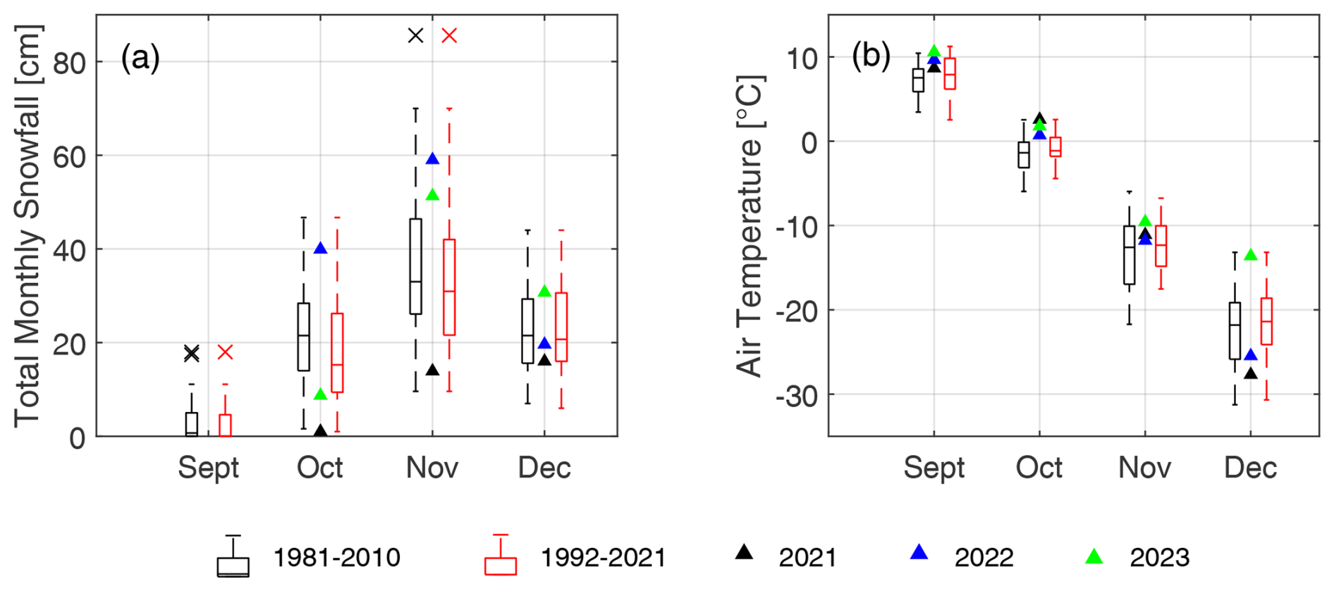
Figure 3 Comparison of (a) cumulative monthly snowfall and (b) mean daily air temperatures for the September–December period in 2021, 2022, and 2023 against the climate normal (1981–2010) and preceding 30-year record (1992–2021) periods.

Table 1 Comparison of air temperatures and snowfall between 2021, 2022, and the 1981–2010 climate normal.

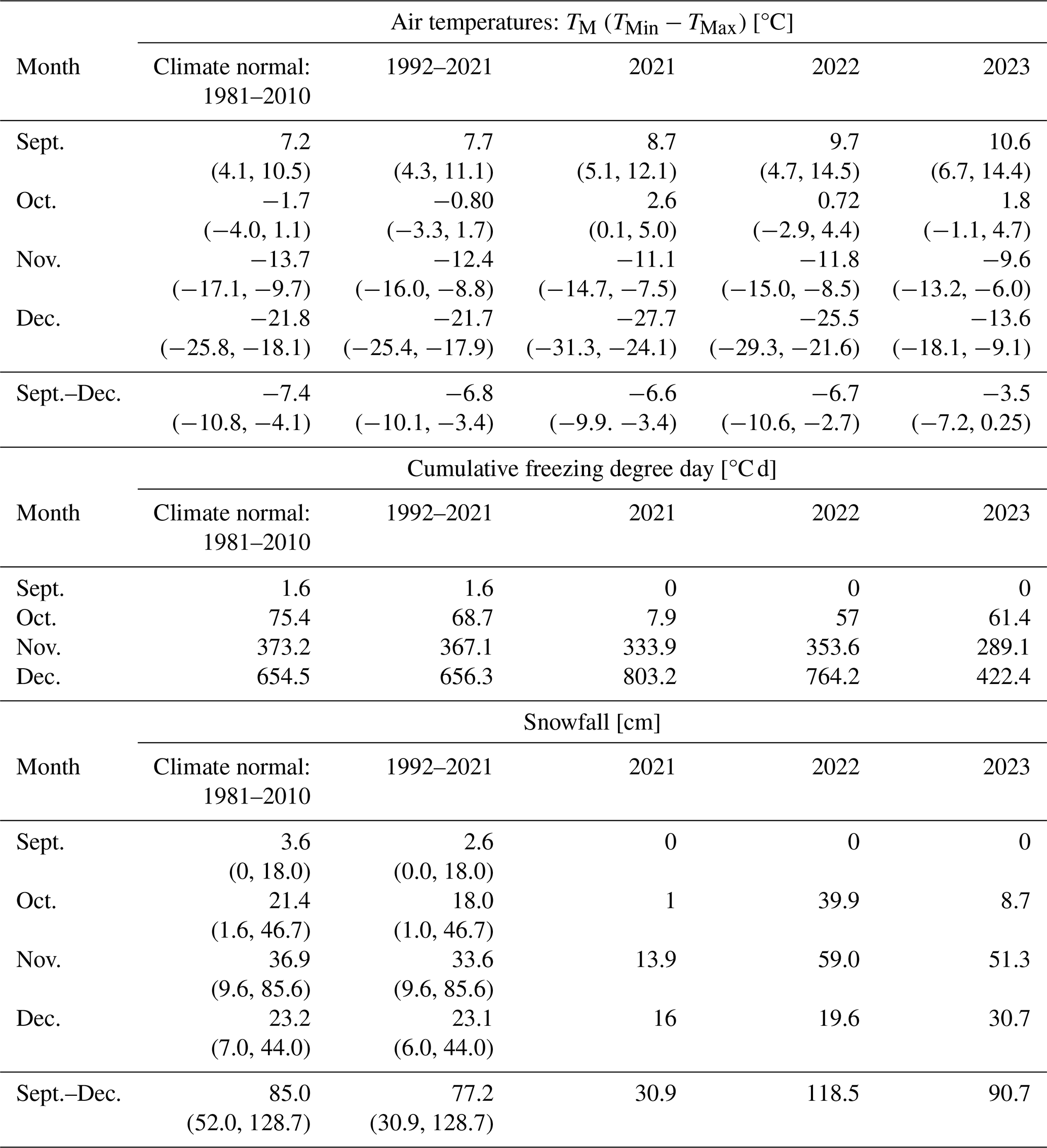
Values in parentheses represent the minimum and maximum monthly cumulative snowfall or daily air temperature in each reference period.

Except for December 2021 and 2022, CFDD in all months between September and December 2021–2023 was lower than normal, indicating warmer-than-normal conditions. October 2021 was particularly warm (and dry), having CFDD=7.9 °C d (Table 1). The same year saw colder-than-normal conditions by the end of December, with CFDD=803.2 °C d (123 % of normal). In 2023, conditions were exceptionally warm, resulting in end-of-December CFDD=422.4 °C d, reaching only 65 % of normal.

Snowfall between September and December 2021–2023 was highly variable (Fig. 3, Table 1). October 2021 had nearly no snow (1 cm), while October 2022 and 2023 had 39.9 and 8.7 cm, respectively. S_T by the end of October 2021 was only 4 % of normal, while October 2022 was 186 % (39.9 cm). Similar variability was recorded in November 2021, 2022, and 2023, having 13.9, 59.0, and 51.3 cm (38 %, 160 %, and 139 % of normal), respectively. The year 2021 was dry, with only 30.9 cm of snowfall falling over the entire September–December period, compared to 85.1 and 77.3 cm for the climate normal and 1992–2021 periods, respectively. This resulted in the second-lowest recorded October S_T, surpassed only by October 1944, which had a total recorded snowfall of 26.1 cm. Between September and December 2022, S_T was 118.5 cm or 139 % and 153 % of the climate normal (85.0 cm) and preceding 30-year periods (77.2 cm), respectively. In 2023, S_T was 90.7 cm, or 107 % and 117 % relative to the same periods, respectively. On a monthly basis, October and November of 2022 had the largest difference from the respective climate normal S_T, being 186 % (39.9 cm) and 160 % (59.0 cm) of their respective climate normal (21.4 and 36.9 cm).

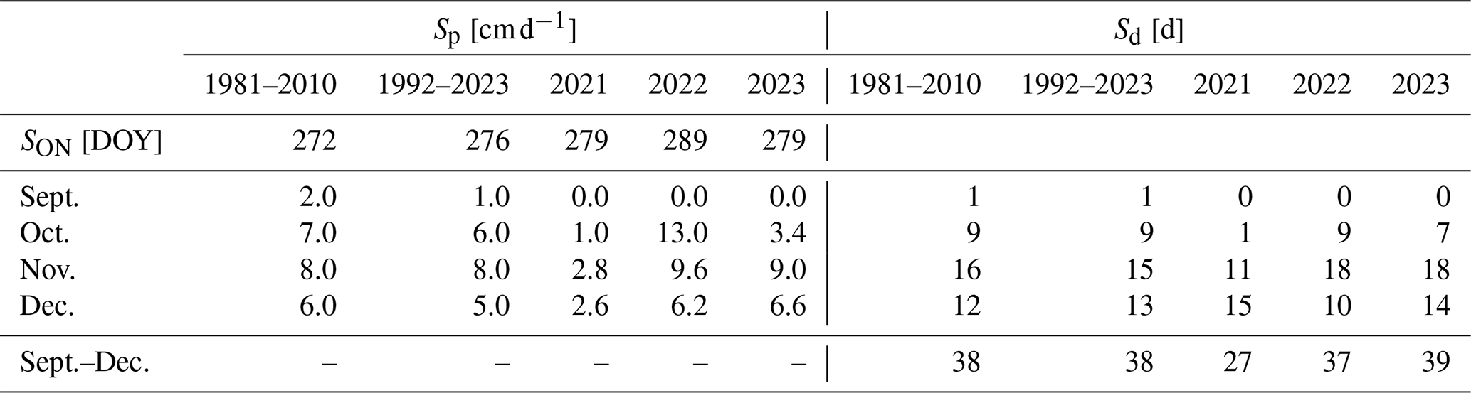
Interannual variability in total monthly snowfall can be decomposed into variability in total number of snowfall days per month (S_d) and the maximum daily snowfall magnitude in each month (S_p). Both parameters can be contextualized for each season by evaluating the timing of the first snowfall of a given winter (S_ON). The values of S_d, S_p, and S_ON are presented in Table 2.

Table 2 Interannual variability in daily snowfall, the number of snowfall days in each month, and the timing of the first winter snowfall.

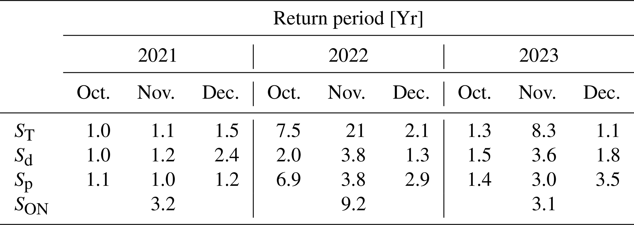
A frequency analysis of snowfall parameters showed return periods of less than 10 years (Fig. 4, Table 3). A notable exception is for the total monthly snowfall in November 2022, where a return period of 21 years was estimated. Figure 4 plots fitted LP3 distributions for each of the snowfall parameters for October, November, and December. September snowfall parameters were neglected as snowfall in September is on average insignificant.

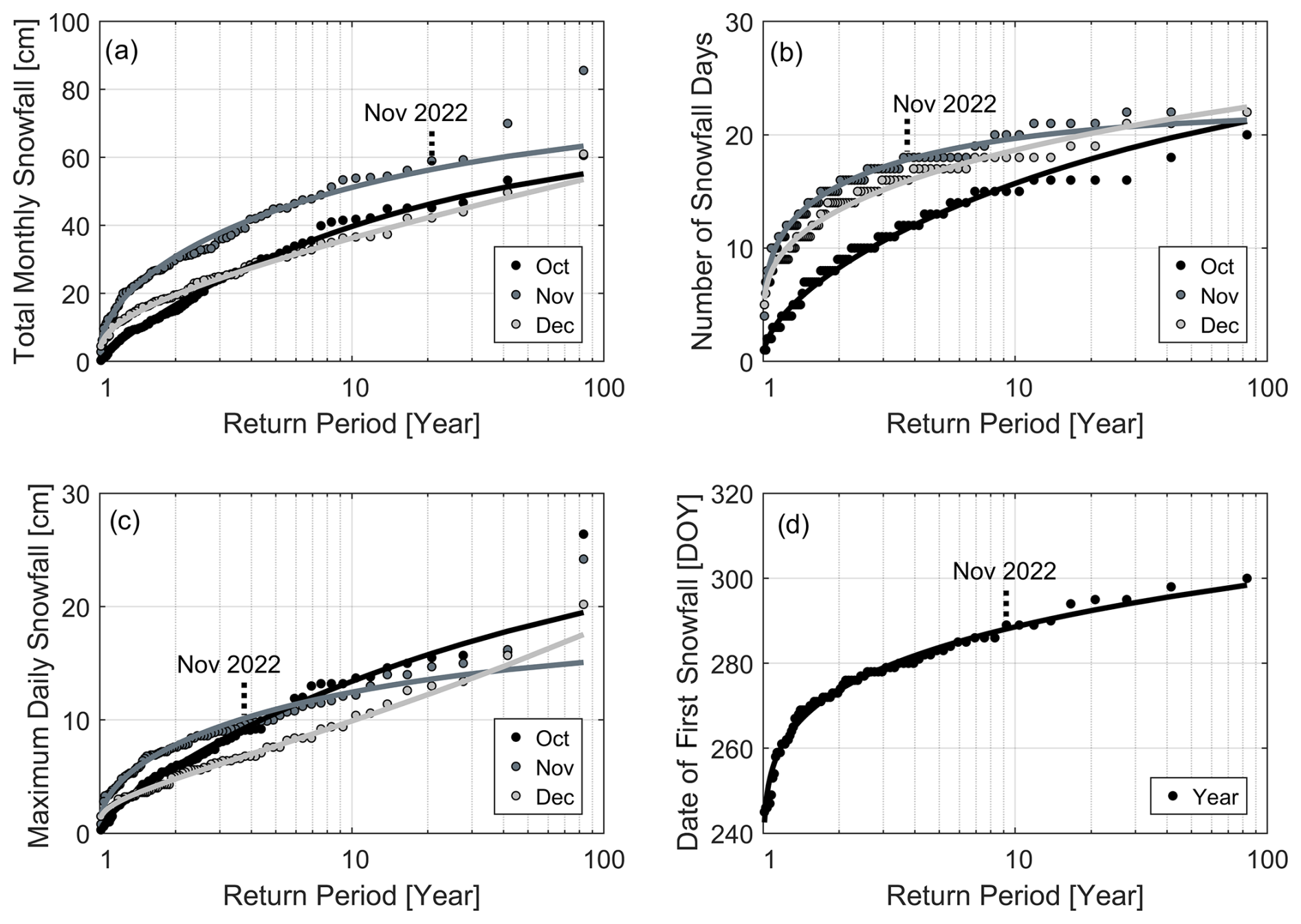
Figure 4 Frequency analysis of snowfall parameters: (a) total monthly snowfall, (b) number of snowfall days, (c) maximum daily snowfall magnitude, and (d) timing of the first snowfall of the year. Log-Pearson Type III distributions (lines) are fit to observations (circles). Each circle represents observations in any given year for October, November, and December.

Table 3 Return period for snowfall parameters recorded in 2021, 2022, and 2023 compared to the historical record (1942–2023).

Log-Pearson Type III (LP3) distributions showed excellent fits to the observed data for all snowfall parameters. Errors generally increased with increasing R_P. For S_T, root mean square errors (RMSEs) ranged from 1.91 to 3.00 cm. S_P had a relatively low RMSE of 0.38–1.10 cm d⁻¹ but increased for R_P>10 years where fewer data existed. Fitted distributions in all months, when averaged, had accuracies in S_d values within 5 d of observations. However, there is a large variability between years, resulting in the assignment of multiple return periods for the same number of snowfall days (Fig. 4b). The first day of recorded snowfall in any given winter was accurately represented using the LP3 distribution, with an RMSE of 1.50 d.

4.2 Freeze-up

The timings of ice onset (IO) and freeze-up dates (FUDs) between 2021 and 2023 were highly variable (Table 4). Between 2021 and 2022, IO varied by 20 d, while FUDs varied by 15–17 d. In 2021, IO was estimated to occur on 1 November, with the FUD occurring between 7 and 9 November 2021. T_M, recorded at the Yellowknife Airport weather station, first fell below freezing overnight on 8 October. Diurnal variability above and below 0 °C in hourly T_a likely led to significant lake cooling, which was expected to have had warmer-than-normal water temperatures based on above-average September and October T_a. MODIS-derived surface temperatures during October 2021 supported this claim, ranging between 1.7–8.8 °C between 3 and 23 October. A notable cooling event likely occurred on 18 October when hourly air temperatures reached a low of −5.4 °C. Despite frequent sub-freezing temperatures, mean daily T_a remained >0 °C, with the exception of 11 October (−0.6 °C) and 18 October (−1.1 °C), until the zero-degree isotherm was crossed on 29 October (Fig. 5a). A lag time of 3 d was observed between the crossing of the zero-degree isotherm and IO. The lag time extended to ∼10–13 d for the FUD, with an uncertainty of 2–3 d.

Table 4 Interannual variability in freeze-up duration, date, and ice onset.

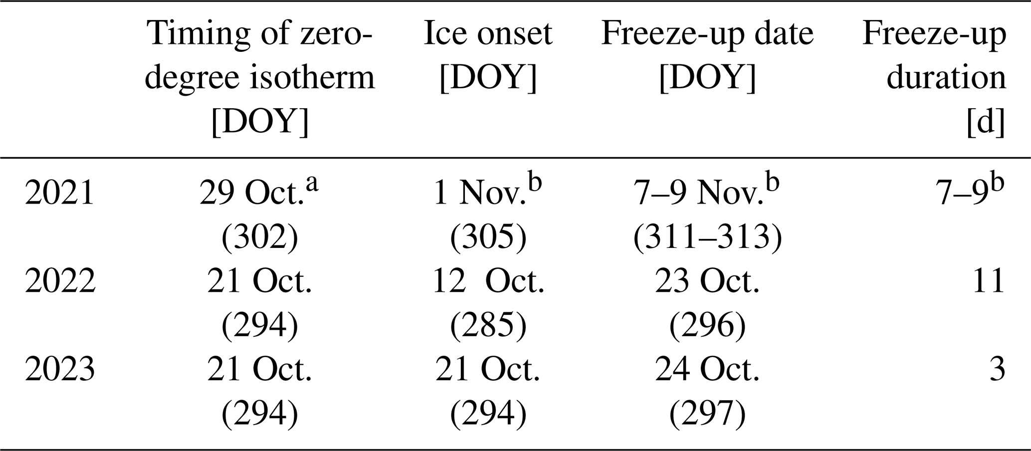
^a Measured by the Yellowknife Airport weather station.
^b Estimated ice onset and freeze-up dates based on Sentinel 2 imagery and MODIS-derived surface temperatures.

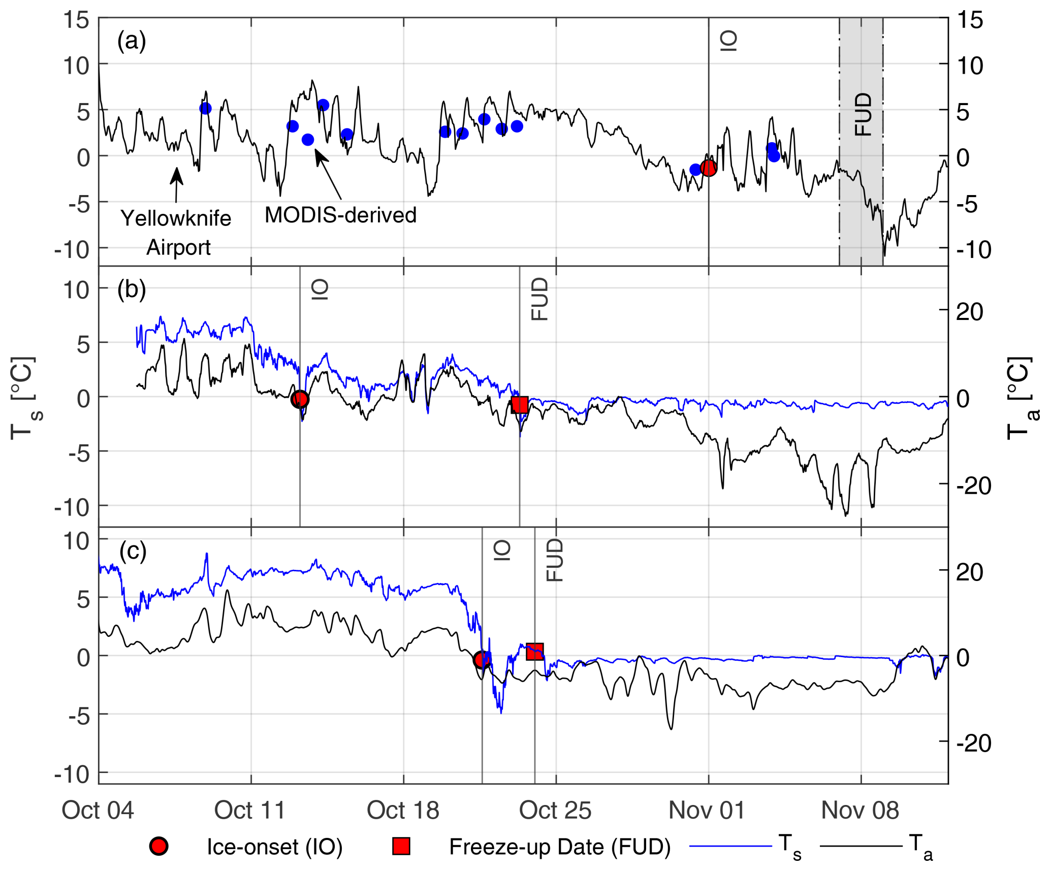
Figure 5 Interannual variability in ice onset (IO) and freeze-up dates (FUDs) between (a) 2021, (b) 2022, and (c) 2023. Air temperatures (T_a) and surface temperatures (T_s) measured by SIMBA are presented as black and blue lines, respectively. Note that in (a), MODIS-derived T_s and air temperatures obtained from the Yellowknife Airport weather station are presented, as no SIMBA was installed prior to 6 December 2021. The grey window in (a) represents a 2 d uncertainty in the FUD in 2021. Surface temperatures in 2022 and 2023 were measured directly by SIMBA by noting the temperature reading at the identified air–water interface along the SIMBA thermistor chain.

In 2022, IO occurred on 12 October (Fig. 5b). Diurnally oscillating air temperatures above and below freezing from 12 to 21 October caused a series of freeze–melt cycles over 11 d, culminating in a FUD of 23 October 2022, 3 d following the crossing of the zero-degree isotherm. Lake surface temperatures closely followed changes in air temperatures until the FUD, where the surface remained slightly below freezing, while air temperatures varied between −27.5 and −0.1 °C. The freeze-up duration was 11 d. In 2023, no freeze–melt cycles were recorded prior to the FUD (Fig. 5c). Air temperatures reached slightly below freezing on only two occasions before crossing the zero-degree isotherm on 21 October 2023: 6 October at 01:30 LT (−0.38 °C) and 17 October 02:30 LT (−0.62 °C). Ice onset coincided with the crossing of the zero-degree isotherm on 21 October 2023. Note that in 2022 and 2023, air temperatures presented here were measured directly by SIMBAs, but in 2021, air temperatures were measured at the Yellowknife Airport weather station. A summary of IO dates, FUDs, and freeze-up durations in 2021, 2022, and 2023 is presented in Table 4.

The zero-degree isotherm was crossed on the same date in 2022 and 2023 (21 October), yet IO dates differed by 9 d. Mean daily air temperatures in the first 2 weeks of October 2023 were significantly lower than in 2022 (Fig. 6a). Mean water ($\stackrel{\mathrm{‾}}{T_{\mathrm{w}}}$) and surface temperatures remained similar until 12 October. Between 4 and 11 October, differences in $\stackrel{\mathrm{‾}}{T_{\mathrm{w}}}$ between 2022 and 2023 ($\mathrm{\Delta }\stackrel{\mathrm{‾}}{T_{\mathrm{w}}}$) were <0.9 °C (Fig. 6b). Changes in heat storage $\left(\dot{E}\right)$ varied between −320.9 and 322.6 W m⁻² in 2022 and between −442.4 and 249.0 W m⁻² (unsmoothed) in 2023. Between 10 and 18 October, $\mathrm{\Delta }\stackrel{\mathrm{‾}}{T_{\mathrm{w}}}$ began to diverge significantly as $\stackrel{\mathrm{‾}}{T_{\mathrm{w}}}$ in 2023 remained high (6.00–7.60 °C), slightly warming between 10 and 14 October. $\stackrel{\mathrm{‾}}{T_{\mathrm{w}}}$ in 2022 declined, beginning on 10 October at a mean rate of 1.24 °C d⁻¹ or 0.30 °C per degree decrease in $\stackrel{\mathrm{‾}}{T_{\mathrm{a}}}$. Warming $\stackrel{\mathrm{‾}}{T_{\mathrm{w}}}$ in 2023 led to a slight net energy gain in the water column (10.4–38.4 W m⁻²), while rapid losses were observed in $\stackrel{\mathrm{‾}}{T_{\mathrm{w}}}$ and T_s in 2022. Differences in $\dot{E}$ between 2022 and 2023 peaked on 12 October at 184.4 W m⁻². A maximum $\mathrm{\Delta }\stackrel{\mathrm{‾}}{T_{\mathrm{w}}}=\mathrm{5.25}$ °C between 2022 and 2023 was observed on 16 October (Fig. 6b).

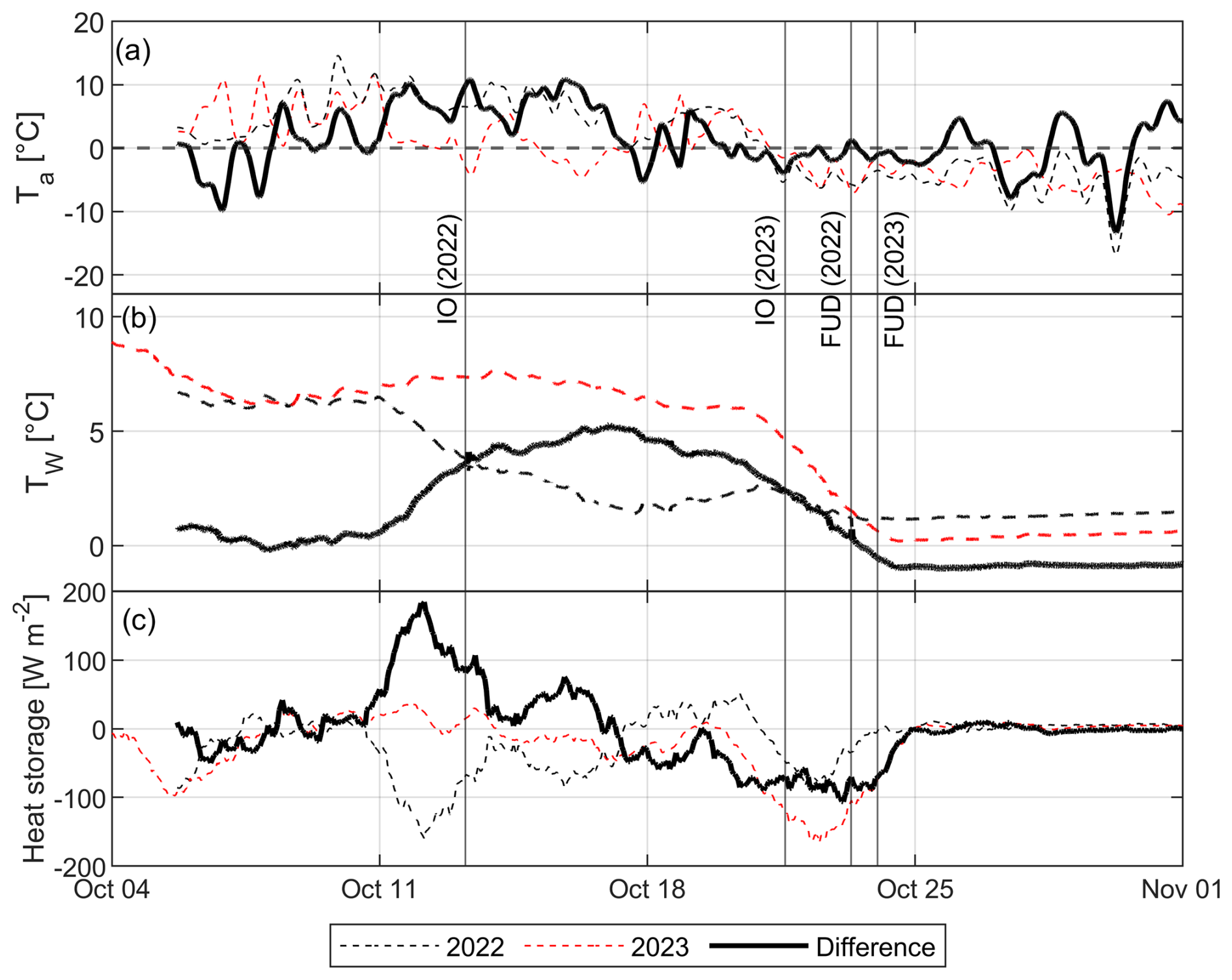
Figure 6 Variability in (a) 15 min air temperatures (T_a), (b) mean water temperatures ($\stackrel{\mathrm{‾}}{T_{\mathrm{w}}}$), and (c) mean hourly heat storage in 2022 and 2023, recorded at the FRS. Values in (a) and (c) are smoothed over a 1 d period. The solid black line represents the difference in water or air temperatures between 2022 and 2023.

$\stackrel{\mathrm{‾}}{T_{\mathrm{w}}}$ remained elevated in 2023 until 20 October. $\stackrel{\mathrm{‾}}{T_{\mathrm{w}}}$ began to decline at a rate of 1.45 from 6.00 °C on 20 October to 0.20 °C on 24 October, with surface temperatures falling below zero on 21 October 2023, leading to the first appearance of ice. Note that $\stackrel{\mathrm{‾}}{T_{\mathrm{w}}}$ was not available in 2021.

In all years, the formation and progression of the ice cover during freeze-up occurred in a similar fashion. Ice first appeared as border ice in the shallower southern sections of Landing Lake and along the shoreline. Mean lake depths in these southern arms were typically less than 1.5 m (Fig. 1). The ice front progressed inwards from the shoreline and northward towards the deeper, central body of the lake until the entire lake was ice covered.

4.3 Evolution of ice and snow

Ice and snow evolutions in 2021, 2022, and 2023 were distinct. In 2021, ice growth following freeze-up was extremely fast: ∼6–8 cm per week as a result of low snowfall (Table 1; Rafat et al., 2023). Ice thicknesses reached 10 cm on 15 November, ∼6–8 d after the FUD (Table 5). Ice growth remained fast as dry conditions persisted in November 2021, with only 14.9 cm of cumulative snowfall having been recorded by the end of November 2021 and manually measured snow depths <10 cm. A total of 30.9 cm of snowfall was recorded by 31 December 2021. The ice thickness reached 30 cm 31–33 d after the estimated FUD and 52 cm by 1 January 2022.

Table 5 Comparison of ice evolution, 2021–2023.

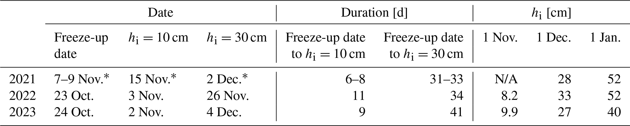
^∗ Interpolated values before the deployment of SIMBA on 6 December 2021.

IO and FUDs in 2022 were significantly earlier (∼2 weeks) than in 2021; however, freeze-up durations were similar (11 vs. 7–9 d). Earlier IO in 2022 did not result in thicker ice when compared to recorded ice thicknesses in December 2021 due to high snowfall and deeper snow on Landing Lake (Fig. 7a). The duration between the FUD to h_i=30 cm in 2022 was nearly identical to 2021, as were the ice thicknesses recorded on 1 December and 1 January (Table 5). Cumulative snowfall in 2022 surpassed 30.9 cm (cumulative snowfall up to 31 December 2021) on 29 October 2022, only 6 d following the FUD. Freeze-up occurred quickly in 2023, taking 3 d from IO to the FUD. Cumulative snowfall values were greater than in 2021 but less than in 2022. However, snow depths recorded on Landing Lake were significantly higher than in 2022 (Fig. 7a) from frequent slushing events that were recorded following freeze-up in 2022, resulting in relatively shallow snow depths and from snow redistribution effects. Ice thicknesses were lower in 2023 than in both 2022 and 2021. CFDD was greater than in 2021 in October and most of November but lower than in 2022. In December, warm air temperatures resulted in a significant reduction in CFDD by the end of the month (Table 1). Low CFDD and moderately high snowfall resulted in low ice thicknesses and slow ice growth, taking 41 d for ice thicknesses to reach 30 cm from the FUD and only growing 13 cm in December.

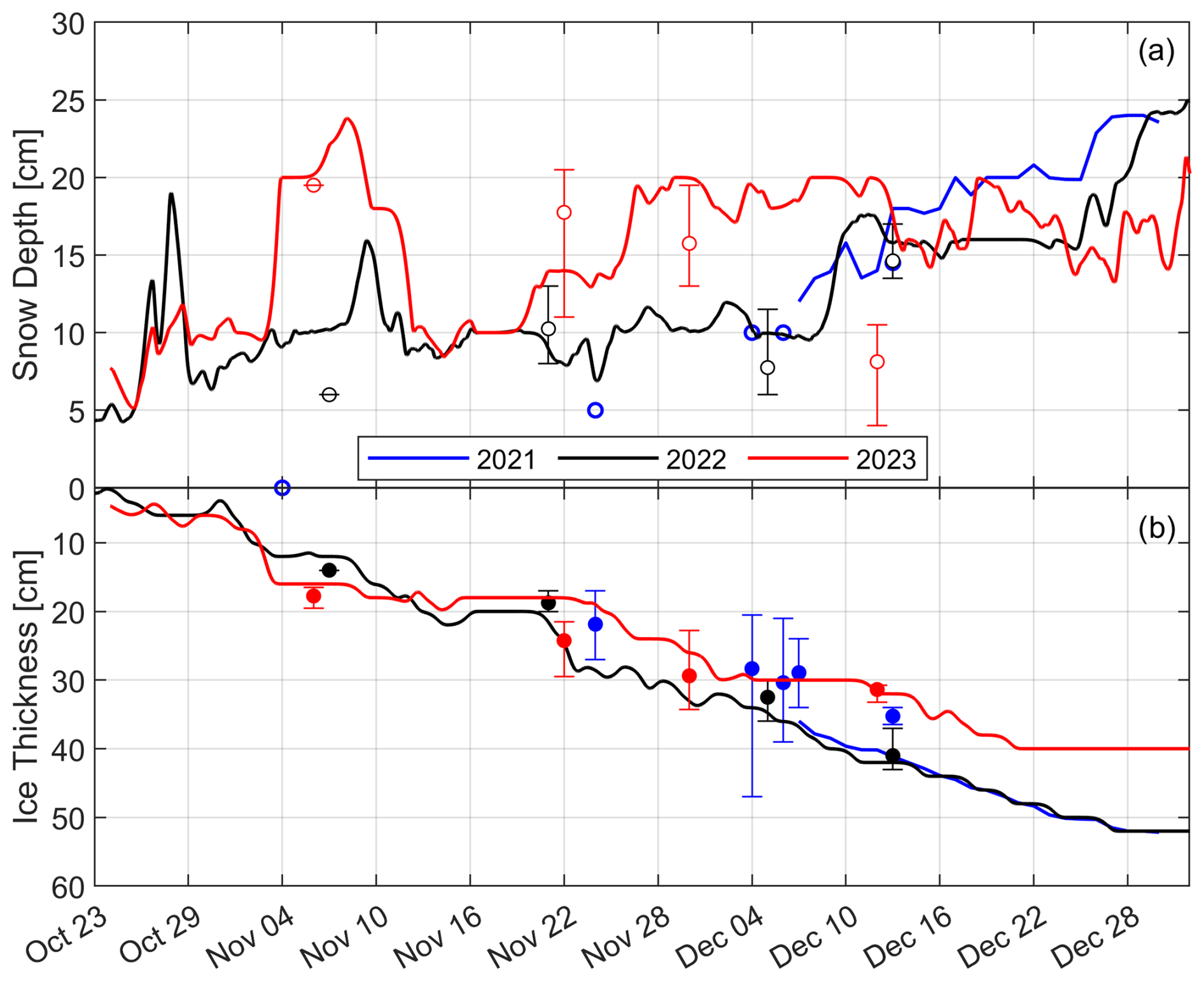
Figure 7 SIMBA-derived (a) snow and (b) ice evolution in Landing Lake in 2021, 2022, and 2023 from the freeze-up date to 31 December. Open and closed circles represent the mean value of manual measurements of snow and ice, respectively. Error bars show measured spatial variability around SIMBA. Ice and snow measurements are smoothed over a 3 d sliding window.

4.4 Relating air, snow, and ice evolution

Variability in air temperatures and snow resulted in three unique responses in the timings of IOs, FUDs, and the growth of ice. The year 2021 was classified as a high-CFDD, low-snowfall year. Meanwhile, 2022 showed near-normal (±15 % of 1981–2010 climate) CFDD but showed above-average (>15 %) S_T. Finally, 2023 presented the case where end-of-December S_T was 106 % of normal but end-of-December CFDD was only 74 % of normal. The effects of air temperature on ice growth are commonly represented using Stefan's equation (Eq. 5a). CFDD was observed to have an exponential relationship with S_T in the form of Eq. (5b). Hence, ice thicknesses may be explicitly modelled as an exponential function of snowfall (Eq. 5c) and indirectly as a function of time. Equation (5c) may be further simplified into a two-constant model by setting $C=\mathit{\alpha }\left(\sqrt{\frac{\mathrm{2}{k}_{\mathrm{i}}}{{\mathit{\rho }}_{\mathrm{i}}L}}\right)\mathit{\gamma }$, such that Eq. (5c) becomes $h_{\mathrm{i}}=C{e}^{\mathrm{0.5}b{S}_{\mathrm{T}}}$ (Eq. 6). α was determined by minimizing the root mean square error (RMSE) of modelled and measured ice thicknesses in 2021, 2022, and 2023.

$$\begin{array}{}\text{(5a)}& {\displaystyle }{h}_{\mathrm{i}}=\mathit{\alpha }\sqrt{{\displaystyle \frac{\mathrm{2}{k}_{\mathrm{i}}}{{\mathit{\rho }}_{\mathrm{i}}L}}\cdot \text{CFDD}}\text{(5b)}& {\displaystyle }\text{CFDD}=\mathit{\gamma }{e}^{b{S}_{\mathrm{T}}}\text{(5c)}& {\displaystyle }{h}_{\mathrm{i}}=\mathit{\alpha }\left(\sqrt{{\displaystyle \frac{\mathrm{2}{k}_{\mathrm{i}}}{{\mathit{\rho }}_{\mathrm{i}}L}}}\right)\mathit{\gamma }{e}^{\mathrm{0.5}b{S}_{\mathrm{T}}}\end{array}$$

$$\begin{array}{}\text{(6)}& h_{\mathrm{i}}=C{e}^{\mathrm{0.5}b{S}_{\mathrm{T}}}\end{array}$$

Equations (5c) and (6) do not explicitly include a melt or retardation factor to account for air temperatures >0 °C and consider IO equivalent to FUDs. Hence, sub-zero air temperatures that occur well before observed FUDs (as in 2021 and 2022) result in modelled FUDs being well in advance of observed FUDs. To account for latency effects, the baseline temperature (BT) for which CFDD is calculated was reduced from 0 to −10 °C in order to select an optimal BT that minimizes errors in FUDs. Variations in the value of all constants under varying BTs are presented in Table 6, and errors in FUDs are presented in Fig. 8.

Table 6 Sensitivity of modelled FUD, α, and RMSE to CFDD baseline temperature (BT) (°C).

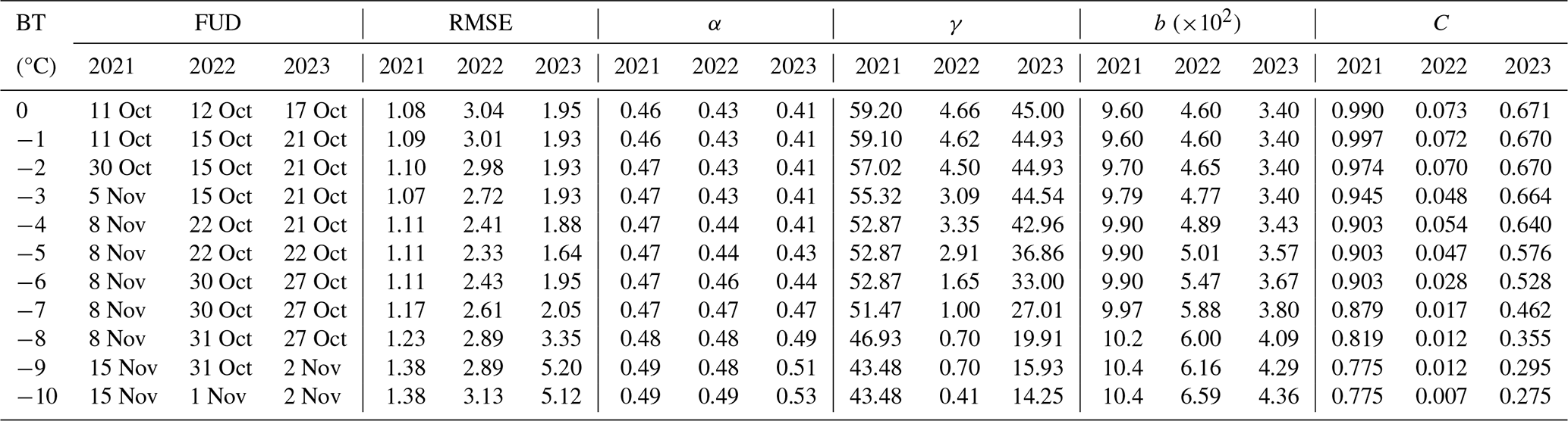
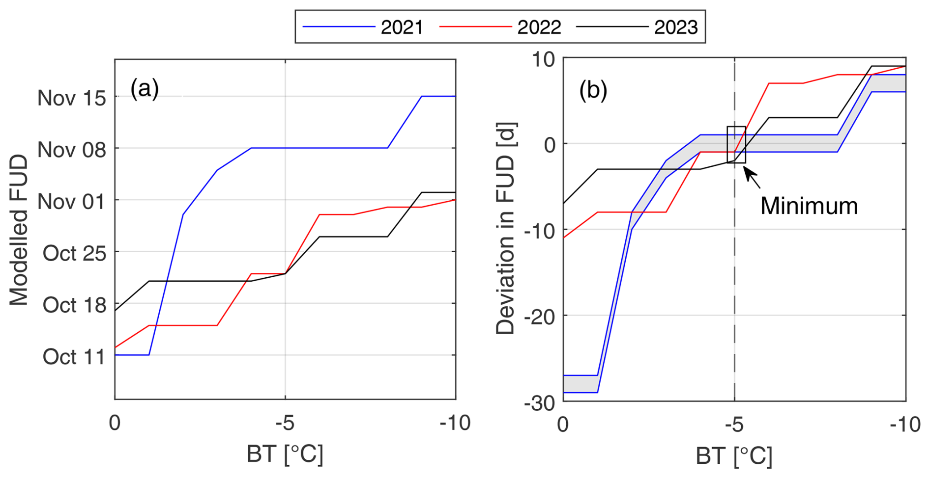
Figure 8 Effects of shifting baseline temperature (BT) on (a) modelled FUDs and (b) deviations between modelled and observed FUDs. The shaded grey region represents the uncertainty in FUD sensitivity to BT from uncertainties in the estimated FUD in 2021.

α showed no sensitivity for decreasing CFDD BT from 0 to −5 °C but linearly increased from −5 to −10 °C. The greatest sensitivity was observed in 2023 in the range −5 to −10 °C, with α increasing by an average of 4.9 % °C⁻¹ reduction in BT. Sensitivity in 2021 and 2022 was marginal but slightly greater than in 2022. γ showed a strong decreasing trend with decreasing baseline temperatures across all years. b showed slight increasing trends with decreasing baseline temperatures over the entire range of tested BT. The magnitude of C decreased with decreasing BT across all years (Table 6).

$\text{BT}=-\mathrm{5}$ °C was selected as it provided the lowest error (RMSE and deviation) in modelled versus observed h_i and FUDs in the range of $-\mathrm{10}\mathrm{°}\mathrm{C}\le \text{BT}<\mathrm{0}\mathrm{°}\mathrm{C}$ (Fig. 8). Optimized values of α, γ, b, and C for the years 2021, 2022, and 2023 are summarized in Table 7. The finalized empirical model using $\text{BT}=-\mathrm{5}\mathrm{°}\mathrm{C}$ is presented in Fig. 9. RMSE between modelled and measured ice thicknesses was small (≤2.33 cm) and deviations in FUDs≤2 d.

Table 7 Constants for the CFDD model using $\text{BT}=-\mathrm{5}$ °C.

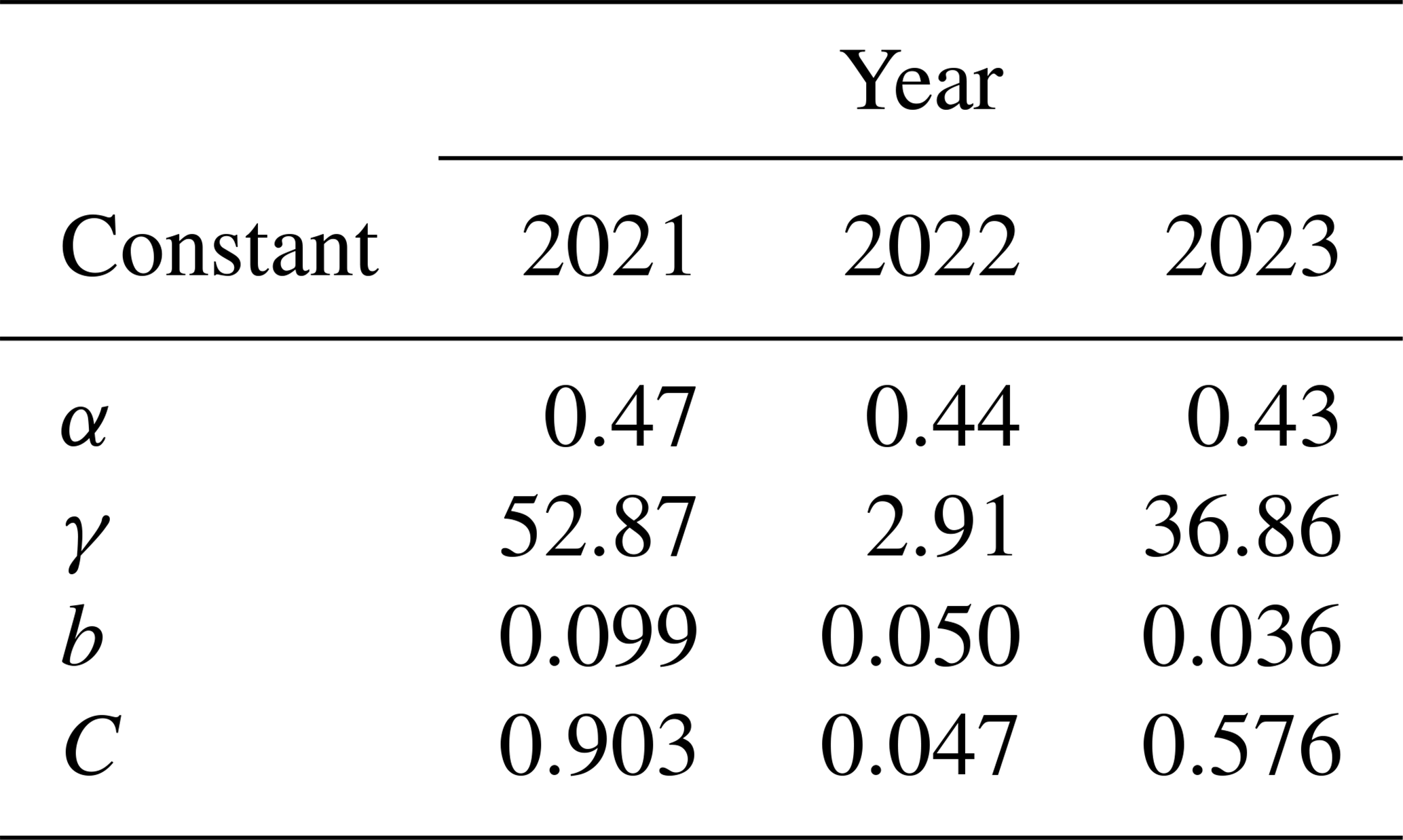
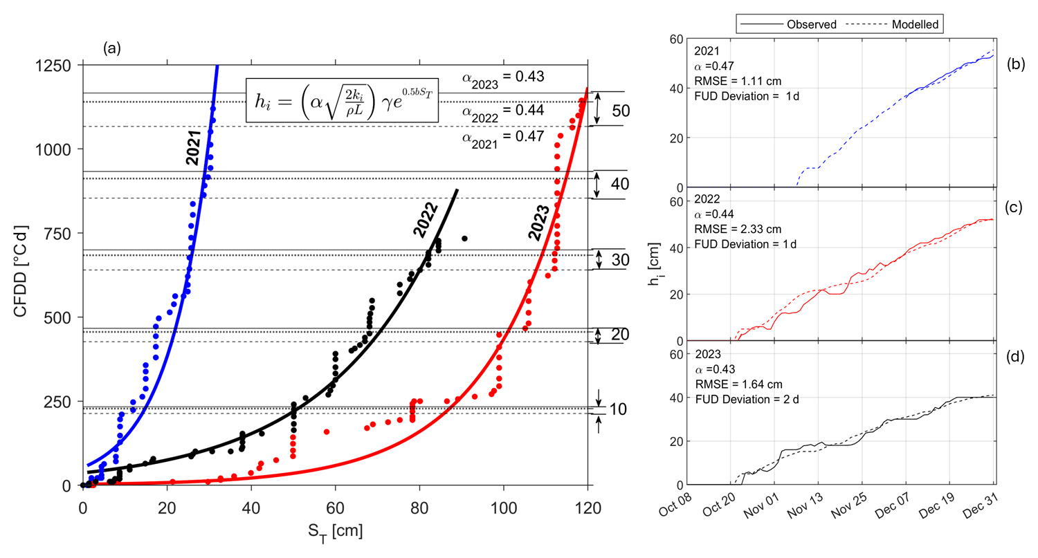
Figure 9 Relationships between cumulative freezing degree days (CFDDs), cumulative snowfall (S_T), and ice thicknesses (h_i) for 2021 (blue), 2022 (red), and 2023 (black). Dashed, solid, and dotted horizontal lines in (a) represent values of α in the years 2021, 2022, and 2023, respectively. Dashed and solid lines in (b)–(d) represent modelled and measured ice thicknesses, respectively. Points represent values of CFDD and S_T recorded at the Yellowknife Airport weather station.

α and b from the model decreased with lower values of CFDD at the end of December and generally decreased with increasing S_T. The sensitivity of α and b to S_T is not linear, however, as α and b in 2022 were slightly larger than in 2023 despite end-of-December S_T in 2022 being larger than in 2023. α and b were observed to decrease consistently with increasing h_s and snow ice (h_si).

h_s was linearly related to S_T in all years (Fig. 10). Correlations were strongest in 2021 (r²=0.82) and 2023 (r²=0.75) and the weakest in 2022 (r²=0.59). Both 2022 and 2023 had mean proportions of snow ice to total ice $\left(\frac{h_{\text{si}}}{h_{\mathrm{i}}}\right)$ of 18 % (0 %–54 %) and 33 % (0 %–44 %). The correlation between h_s and S_T was stronger in 2023 than in 2022, despite $\frac{h_{\text{si}}}{h_{\mathrm{i}}}$ being greater in 2023. Moderately positive correlations (r²=0.50, 0.67, and 0.76 for 2021, 2022, and 2023, respectively) were also observed between h_s and h_i.

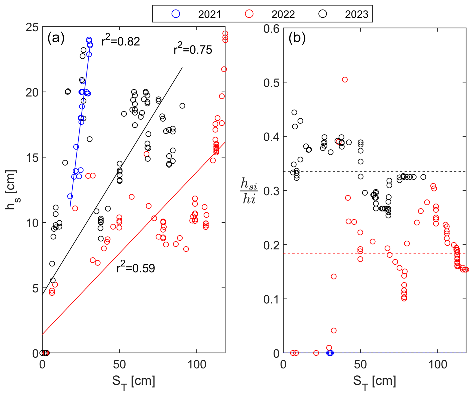
Figure 10 Correlations between (a) snow depths and (b) proportions of snow ice to total ice against total snowfall.

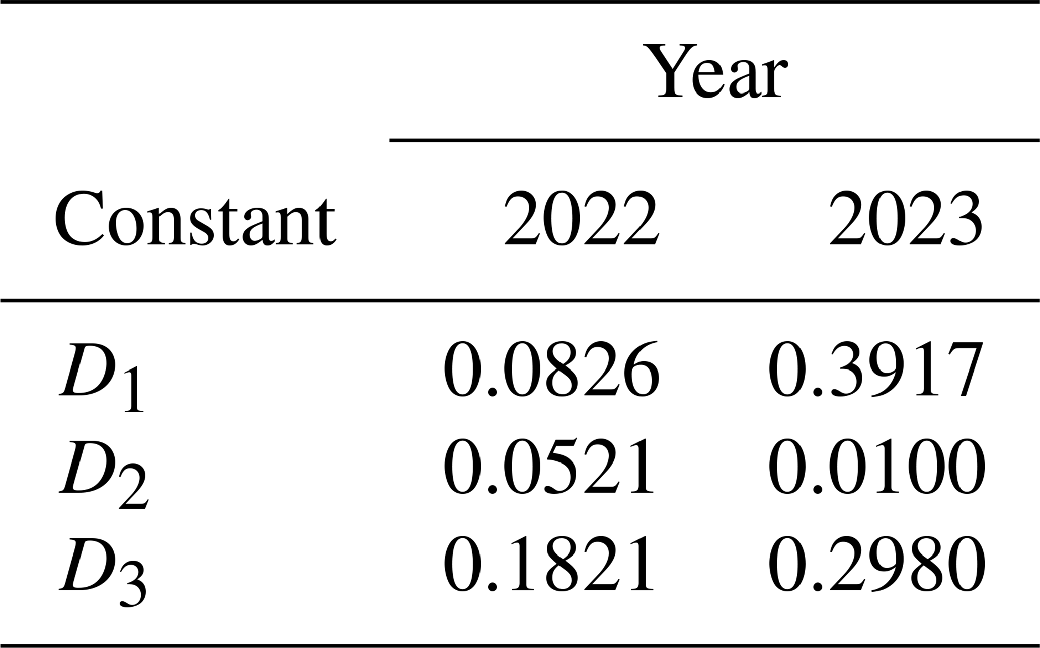
h_si in both 2022 and 2023 could be effectively reproduced using a simple multi-linear regression model in the form of $h_{\text{si}}=D_{\mathrm{1}}+D_{\mathrm{2}}{S}_{\text{day}}+D_{\mathrm{3}}{h}_{\mathrm{i}}$. The model consisted of three constants (D₁, D₂, and D₃) and only two variables: daily snowfall (non-cumulative, S_day) and h_i. (Fig. 11). Using the model, RMSEs in 2022 and 2023 compared against measured h_si were 1.21 and 0.81 cm, respectively. The accuracy of the simulations was further evaluated using the Nash–Sutcliffe efficiency (NSE) parameter, with both years showing excellent simulation strength (NSE=0.86 and 0.95 for 2022 and 2023, respectively). The values of constants D₁, D₂, and D₃ are presented in Table 8.

Figure 11 Modelled versus observed snow ice thicknesses.

Table 8 Value of constants for the linear snow ice model.

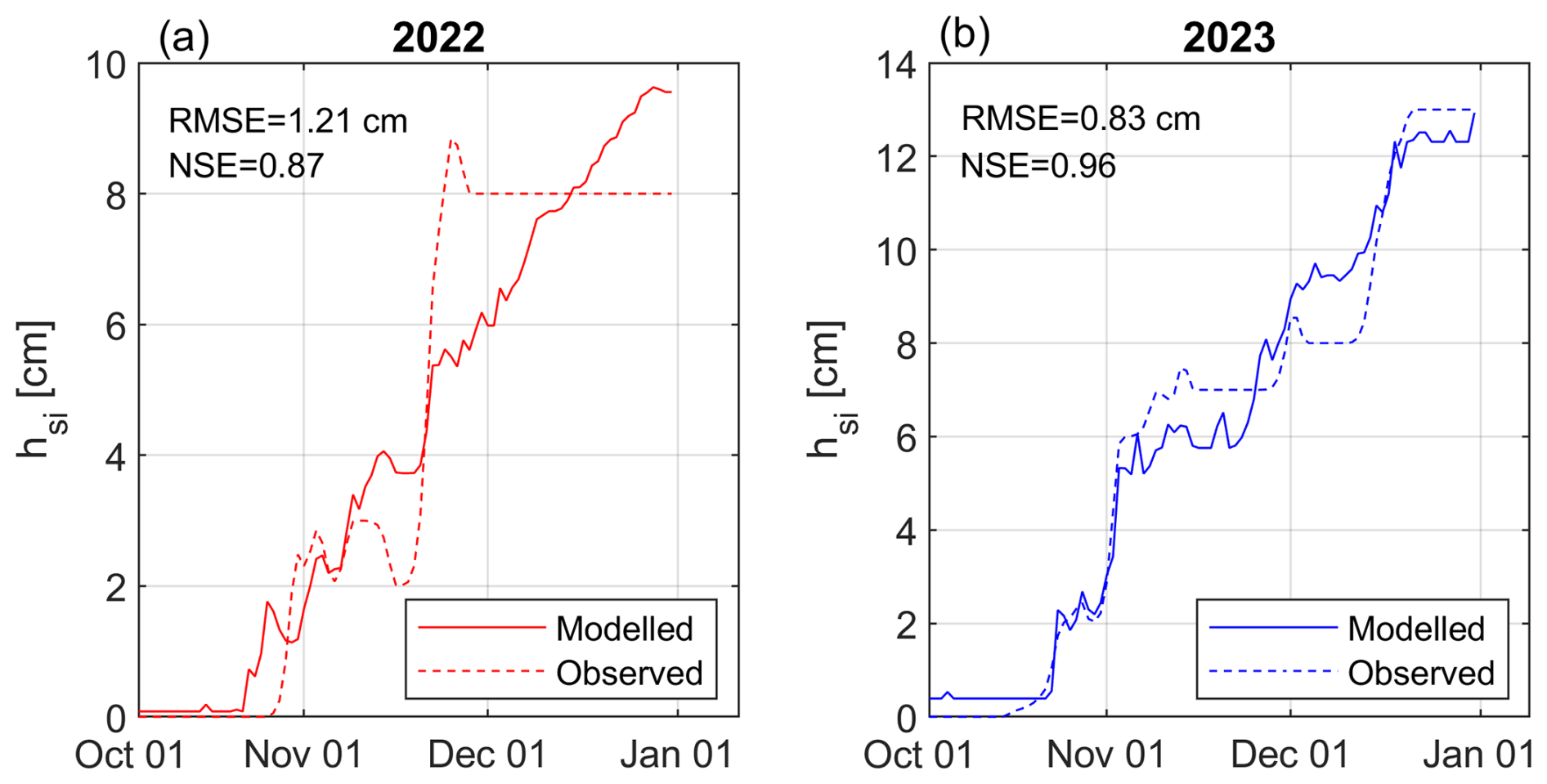
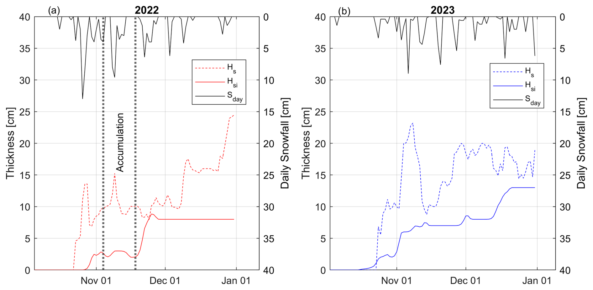
h_si was more accurately simulated in 2023 compared to 2022. In 2023, higher snowfall was closely followed by snow ice formation (Fig. 12b), suggesting near-critical submergence conditions (low freeboard). This contrasts with 2022, where between 4 and 18 November 23.1 cm of snowfall was recorded but no snow ice was produced (Fig. 12a), suggesting that ample freeboard was present in the ice cover to support significant snow loading without submergence. This phenomenon is reflected in Fig. 12a where modelled h_si was not able to accurately capture the rapid snow ice formation between 19 and 25 November when the available freeboard was thought to be exceeded.

Figure 12 Interactions between snowfall, snow depths, and snow ice in (a) 2022 and (b) 2023.

5 Discussion

Variability in air temperatures and snowfall conditions controlled the variability in observed IOs and FUDs. Warmer-than-average T_M and T_Min>0 and predicted warmer-than-normal water temperatures in September and October 2021 dramatically delayed IO and FUD into November (Table 4). In contrast, cooler T_M and earlier cooling of the lake in 2022 resulted in an IO 20 d and 9 d earlier than in 2021 and 2023, respectively. The earlier IO resulted in a prolonged freeze-up duration of 11 d, caused by frequent air temperature variability above and below 0 °C, with T_M remaining >0 °C until the crossing of the zero-degree isotherm on 21 October 2022 (Table 4).

Following FUDs, ice growth was jointly controlled by the effects of air temperatures through CFDDs and snowfall through S_T. Low S_T and high CFDDs following October 2021 resulted in rapid ice growth, evidenced by a 6–8 d duration to reach h_i=10 cm and 31–33 d to reach h_i=30 cm (Table 5). Low S_T during the September–December period in 2021 was explained by a combination of lower-than-normal S_n (11 d) and lower-than-normal S_P (0–2.8 cm h⁻¹) in all months (Table 2). In contrast, the high quantity of snowfall and warmer air temperatures in 2022 (compared to 2021) following the FUD contributed to the increased durations from the FUD to h_i=10 cm (11 d) and h_i=30 cm (34 d). In particular, the effects of snowfall in November 2022 were significant to slowing ice growth, equivalent to a return period of 21 years. Higher-than-normal S_T was explained by higher-than-normal S_P, as S_d remained near-normal and S_ON was 17 d later than normal (Table 2). Although S_n was near-normal, when considering S_d in the context of the number of days between S_ON and 31 December 2022 (77), nearly 1 in 2 ($\mathrm{37}/\mathrm{77}$; 48 %) days had recorded snow. This is significant compared to snowfall occurring twice every 5 d (40 %) for the climate normal period. In 2023, ice growth was significantly hindered from both high S_T and low CFDD.

Using an empirical approach, unique relationships between CFDD, S_T, and h_i were developed (Fig. 9). It was observed that using a $\text{BT}=-\mathrm{5}\mathrm{°}\mathrm{C}$ for calculating CFDD minimized RMSE between modelled and simulated h_i and errors in FUDs (Table 7; Fig. 8). The selection of $\text{BT}=-\mathrm{5}\mathrm{°}\mathrm{C}$ considered latency effects between changes in lake water temperatures and air temperatures. Air temperatures may fall below 0 °C, triggering Eqs. (5c) and (6) to produce ice, yet Landing Lake may still contain ample heat to prevent ice formation. Parameters α and b decreased with decreasing end-of-December CFDD and with increasing h_s and h_si. This finding agrees with the general understanding that α decreases with increasing snow and flow (Michel, 1971; Shen, 2010).

While BT=0 °C is commonly used (e.g., Gow and Govoni, 1983; Michel, 1971), the choice of 0 °C as a threshold for the calculation of CFDD in lakes is arbitrary, with any sub-freezing temperature proving sufficient. Interestingly, here we note that $\text{BT}=-\mathrm{5}\mathrm{°}\mathrm{C}$ provided the lowest RMSE and deviation in h_i and FUD across all years. This baseline is colder than that commonly used for sea ice of $\text{BT}=-\mathrm{1.8}\mathrm{°}\mathrm{C}$ for salinity of 32 ‰ (Bilello, 1961; ISO, 2019). Although only considering ice melt in their analysis, Bilello (1980) provided a through discussion on the use of 0, −1.8, −5, and −10 °C as BTs for evaluating cumulative simulations of ice decay using thawing degree days (CTDD). Bilello (1980) concluded that the use of BT=0 °C was most appropriate for the simulation of break-up using CTDD in lakes and −5 °C in rivers, citing melt occurring before air temperatures rise to 0 °C. The inverse argument can be applied to the freezing process where lakes and rivers do not necessarily freeze immediately following air temperatures falling below 0 °C. It is coincidental that our findings presented the lowest error for CFDD calculated using $\text{BT}=-\mathrm{5}\mathrm{°}\mathrm{C}$, the optimal threshold for CTDD in rivers, as identified by Bilello (1980).

h_s was linearly correlated to S_T in all years. The strongest correlation in 2021 (r²=0.82) was likely attributed to no snow ice being produced and generally low S_T (Fig. 10). Stronger correlations in 2023, where $\frac{h_{\text{si}}}{h_{\mathrm{i}}}$ is greater than in 2022, suggest that snow ice does not account for all observed variability. The remaining variability may be attributed to snow redistribution and metamorphic processes, which can create significant spatial and temporal variability in snow depths (Pouw et al., 2023). Partially unexpected findings of positive correlations between h_s and h_i could be explained by deeper snow slowing ice growth, provided that snow ice is not forming and that density remains constant. The positive correlation alluded to the positive contribution of snow to snow ice formation.

To simulate snow ice, empirical models were developed in this study using a multi-linear regression (Fig. 11). Simulations of h_si were more accurate in 2023 than in 2022. This was likely the result of the ability of the ice cover to support the snow load while maintaining a positive ice freeboard during the time of snowfall (Fig. 12). The addition of a freeboard component to the model would likely improve simulation strength but at a cost of increased complexity and uncertainty as the accurate estimation of freeboard could be challenging.

Estimates of snow ice thicknesses and proportions of snow ice to total ice thickness are significant for (1) estimating future bearing capacity of ice cover and for adaptation of ice road designs, (2) predicting future BUDs, and (3) understanding possible changes to under-ice ecological processes. Following (1), Gold's formula remains the standard approach for bearing capacity estimates for ice road design, with a reduction to the effective ice thickness to compensate for snow ice of lower quality (less dense; Masterson, 2009). Hence, estimates of snow ice proportions may be used (with caution) as a first-order approximation of future changes in load-bearing capacities. However, this approach has limitations. While the strength of snow ice under confinement may be lower than congelation ice, the strength of an ice sheet undergoing bending or punching failure, composed of varying proportions of snow and congelation ice, is not well investigated. Additionally, the effects of varying ice layers on ice flexural strength are thought to be variable (Daly et al., 2023). Note that snow ice may be considered equivalent in strength to congelation ice for densities >880 kg m⁻³ (Masterson, 2009), highlighting the nuances of snow ice in bearing-capacity estimation. There is hence a growing need to revisit and modernize Gold's formula in response to current climate change, perhaps through reproducing large-scale breakthrough testing conducted in Canada prior to the 1960s (Gold, 1960), taking into account ice composition. Future efforts to modernize routine ice road operations may choose to recognize such limitations in Gold's formula (e.g., Fitzgerald and van Rensburg, 2024) and adopt a limit-stress-based approach (Masterson, 2009).

Following (2), greater snow ice thicknesses may delay BUDs in lakes as snow ice effectively scatters insolation and may slow internal melting and deterioration. The rapid deterioration of ice in the spring leads to increasing porosity and rapid collapse of the ice sheet (collapse failure), as was evident during the decay process in Landing Lake in May 2023 (Rafat et al., 2024). Greater snow ice thicknesses may also prevent this failure mechanism through reducing the candling of the ice cover. This effect may be exploited for late-season ice road operations. For instance, one lane of road traffic can be closed and covered with compacted snow or flooded to form snow ice while the other lane is used. Once the active lane is degraded, traffic can be redirected to the snow-ice- or snow-covered lane (upon clearing) (Strandberg et al., 2012). This lane will have its strength properties largely intact due to reduced internal melt and deterioration. Following (3), for snow ice thicknesses greater than 30 cm, the magnitude of photosynthetically active radiation that is able to penetrate the ice cover approaches zero (Kirillin et al., 2012). This directly influences under-ice aquatic ecology through influencing lake mixing and primary productivity (Hampton et al., 2017).

The presented empirical models demonstrate an effective means of simulating total ice and snow ice thicknesses in Landing Lake using snowfall and air temperatures recorded from the Yellowknife Airport weather station, located 11 km south of Landing Lake. Relationships between CFDD and S_T (Fig. 9) can be considered as regional relationships, which can be applied to other Yellowknife-area small lakes with similar lake depths (e.g., <5 m) and surface areas (e.g., <5 km²) for first-order estimates of ice thicknesses. This can be extended across the NWT where ∼138 000 small and shallow lakes and ponds were identified (>0.1 km²), accounting for ∼86 % of all NWT lakes in the HydroLAKES dataset (Messager et al., 2016). To do so, the same methodology would be applied for establishing the values of α γ, b, C, D₁, D₂, and D₃ in other regions of the Northwest Territories, provided that measurements of snowfall and air temperature and a few measurements of ice thickness are available. This analysis is not intended for use in large and deep lakes whose latency effects during freeze-up would require unique treatment. Multi-year monitoring in other regions of the Northwest Territories can aid in establishing regional curves such as those presented in Fig. 9 for determining interannual and regional variability in model parameters.

6 Conclusions

This study investigated the influence of weather on ice evolution in a small and shallow subarctic lake during the early winter periods (September–December) of 2021, 2022, and 2023. Weather variability was characterized using air temperature and snowfall data. Distinct combinations of varying air temperatures and snowfall conditions resulted in three unique responses in the timings of IOs, FUDs, and the growth of ice for 2021, 2022, and 2023, respectively. Variability of up to 20 d in IOs, 17 d in FUDs, and 8 d in freeze-up durations was observed. The duration between FUDs and when ice thicknesses (h_i) reached 30 cm varied between 31 and 41 d, while the timing from FUDs to h_i=10 cm varied between 6 and 11 d. Ice thicknesses on 1 December varied by only 6 cm between the years (27–33 cm) but doubled by 31 December to 12 cm (40–52 cm). Changes in water temperatures closely followed changes in air temperature, which controlled the timing of FUDs, yet the crossing of the zero-degree isotherm was observed as not being a reliable indicator for use in predicting IOs or FUDs.

Variability in ice evolutions between 2021, 2022, and 2023 was effectively explained using an empirically derived model involving cumulative freezing degree days (CFDDs) and snowfall (S_T) in the form of $h_{\mathrm{i}}=\mathit{\alpha }\left(\sqrt{\frac{\mathrm{2}{k}_{\mathrm{i}}}{{\mathit{\rho }}_{\mathrm{i}}L}}\right)\mathit{\gamma }{e}^{\mathrm{0.5}b{S}_{\mathrm{T}}}=C{e}^{\mathrm{0.5}b{S}_{\mathrm{T}}}$, where α, γ, and C are constants. h_i was effectively simulated in all years with RMSE≤2.33 cm, with accuracy in estimated FUDs of ≤2 d when calculating CFDD using a −5 °C threshold. A simple model for the simulation of snow ice thicknesses using CFDD and daily snowfall (S_day) in the form of $h_{\text{si}}=D_{\mathrm{1}}+D_{\mathrm{2}}{S}_{\text{day}}+D_{\mathrm{3}}{h}_{\mathrm{i}}$ proved effective (RMSE≤1.21 cm), where D₁, D₂, and D₃ are fitted constants. Snow depths over lake ice were found to be linearly related to S_T (r²=0.59–0.82), with the strength of the correlations decreasing with increasing S_T. Developed empirical relationships may be site-specific but are a simple and useful means of anticipating ice growth, given the short-term forecasts of snowfall conditions and air temperatures, which can be applied to the small watershed scale.

Under future climate change, winter precipitation and air temperatures in northern Canada are projected to increase (Zhang et al., 2019). Future projections can be used with the presented empirical relationships to understand, to a first order, variability in early winter ice formation and growth for application to ice road design. Empirical relationships between CFDD and S_T may allow engineers to select appropriate construction methods and equipment, establish appropriate quality and hazard control plans, and determine if critical conditions may exist to warrant expanded stress-state analyses or interventions during ice road construction. While the study was conducted in a small lake near Yellowknife, the empirical relationships developed in this study can be adapted to other northern high-latitude regions with similar climatic conditions. Given that CFDD and snowfall are widely monitored meteorological variables, the model framework can be extended for regional-scale assessments with appropriate calibration. This enhances its potential utility for winter road planning and operational decision-making across boreal and subarctic regions facing similar climate challenges.